Extended Laplace Power Series Method for Solving Nonlinear Caputo Fractional Volterra Integro-Differential Equations

Abstract

In this paper, we compile the fractional power series method and the Laplace transform to design a new algorithm for solving the fractional Volterra integro-differential equation. For that, we assume the Laplace power series (LPS) solution in terms of power $q=\frac{1}{m},m\in Z^{+}$, where the fractional derivative of order $\alpha =q\gamma$, for which $\gamma \in Z^{+}$. This assumption will help us to write the integral, the kernel, and the nonhomogeneous terms as a LPS with the same power. The recurrence relations for finding the series coefficients can be constructed using this form. To demonstrate the algorithm’s accuracy, the residual error is defined and calculated for several values of the fractional derivative. Two strongly nonlinear examples are discussed to provide the efficiency of the algorithm. The algorithm gains powerful results for this kind of fractional problem. Under Caputo meaning of the symmetry order, the obtained results are illustrated numerically and graphically. Geometrically, the behavior of the obtained solutions declares that the changing of the fractional derivative parameter values in their domain alters the style of these solutions in a symmetric meaning, as well as indicates harmony and symmetry, which leads them to fully coincide at the value of the ordinary derivative. From these simulations, the results report that the recommended novel algorithm is a straightforward, accurate, and superb tool to generate analytic-approximate solutions for integral and integro-differential equations of fractional order.

1. Introduction

Fractional calculus (FC) is a mathematical discipline that dates back 300 years, defined in the 19th century by Rieman and Liouville as “the generalization of the ordinary derivative to non-integer values”, and was later developed by Euler, Liouville, and Abel (1823). For more details, see [1,2,3]. In recent decades, FC has started to attract much more attention from researchers. It was found that different, particularly interdisciplinary applications can be modeled superbly with the help of fractional derivatives. For instance, robotics, nonlinear oscillations of earthquakes, control theory, signal processing, and viscoelasticity [4,5,6,7]. For more details and applications of FC, we refer the reader to [8,9,10,11,12,13,14]. Since the ordinary differential is a local operator, but the fractional order differential operator is nonlocal, the nonlocal property is considered the most significant aspect of using fractional differential equations (FDEs), which indicates the following state of a phenomenon does not rely only upon its current state but considers its historical states as well. For this reason, FDEs have drawn great attention from researchers for their realism in the interpretation of real-world phenomena and it has become a more popular mathematical discipline. For example, in circuit systems [15], electrochemistry of corrosion [16], heat conduction [17], optics and signal processing [18], probability and statistics [19], inviscid fluid [20], fluid flow [21], and so on. In the literature, eminent researchers have introduced and developed various ways to define fractional derivatives (FD), such as Atangana–Baleanu, Riemann–Liouville, Abel, Weyl, Riesz, Caputo–Fabrizio, and Caputo operators. The Riemann–Liouville and Caputo FDs are the most popular, and they give a high degree of freedom in the description and simulation of the physical phenomena compared with ordinary derivatives. To learn about these FDs, see [22,23,24,25,26,27,28].

Various mathematical formulations of science and engineering phenomena involve linear and nonlinear differential equations, integral equations, or integro-differential equations (DEs, IEs, IDEs) that play a vital role in simulating a wide range of both linear and nonlinear phenomena in varied science and engineering fields. However, when converting these phenomena to either DEs, IEs, or IDEs, some of them are complicated and cannot be treated with the help of ordinary calculus. In this regard, many scientists have concentrated on employing FDEs and fractional IDEs (FIDEs) as convenient tools in modeling the phenomenon, and they play an important role in exploring solutions utilizing varied methods, which is in line with the rapid growth in explaining the various phenomena originating from the natural sciences more accurately than ordinary DEs. Notably, fractional integral and integro-differential equations are qualified for elucidating natural processes adequately in terms of symmetry characteristics. However, there remain challenges to solving the nonlinear models of such phenomena theoretically or numerically. Recently, many researchers have devoted more effective methods to provide a solution, either approximate, analytical, numerical, or exact, to such models. Exploring the analytic solution of FDEs and FIDEs is difficult in most cases, even though abundant efforts have been introduced recently to develop emerging numerical and approximate-analytical techniques for finding out the solutions to linear and nonlinear fractional problems. Among these methods, the kernel Hilbert space method [29], the Haar wavelet method [30], the Adomian decomposition method [31], the homotopy analysis method [32], the finite difference method [33], the Taylor series expansion method [34], the collocation method [35], the Aboodh transform decomposition method [36], and the residual fractional power series (FPS) method [37,38] have been reproduced. The FPS method is one of the semianalytical techniques which befits both linear and nonlinear FDEs [39,40,41]. It has been proposed that the solution is formulated on generalized Taylors series where the coefficients of the expansion could be found by employing FD on the residual error function in each step. To avoid this step, a novel and efficient technique for generating analytic-approximates of wide classes of FDEs has been suggested and named the Laplace fractional power series (LFPS) method [42]. The LFPS approach had been suggested as a modern algorithm which is a mixture of two strong approaches, the fractional power series (FPS) and the Laplace transform (LT). The LFPS algorithm is a considered to be appropriate for handling several linear and nonlinear fractional models and investigating their solutions: such as time-fractional Swift-Hohenberg equations [43], time-fractional Black–Scholes option pricing equations [44], time-fractional Kolmogorov and Rosenau–Hyman models [45], temporal time-fractional gas dynamics equations [46], time-fractional generalized biology population models [47], and fractional reaction–diffusion for bacteria growth models [48].

Motivated by the aforementioned works, this article extends the application of the LFPS method for solving nonlinear FIDEs in the Volterra sense, as shown in the underlying form.

$${\mathfrak{D}}_t^{\alpha }u\left(t\right)=f\left(t\right)+{{\displaystyle \int }}_0^{t}k\left(x-t\right)g\left(u\left(x\right)\right)dx, \alpha \in \left(0,1\right], t\ge 0,$$

(1)

where $\alpha$, is the parameter defining the Caputo-FD, the functions $f\left(t\right)$ and $k\left(x-t\right)$ are continuous real-valued functions, and $g\left(u\left(x\right)\right)$ is the nonlinear function of $u\left(x\right)$. In the Volterra sense, the solution of FIDEs is crucial for describing the pattern of linear and nonlinear physical phenomena, particularly, the phenomena excited in harmony or to evaluate the probabilistic response of randomly-excited analytical models, the dynamics of nuclear reactors, and so forth. A functional expansion of a dynamic, nonlinear, and time-invariant functional is referred to as a Volterra series.

The main contribution of this work is to design a modern modified algorithm to generate the analytic-approximate solutions of the nonlinear fractional Volterra integro–differential equation (FVIDE) in the framework of employing Caputo-FD. This kind of FD is chosen in the present analysis due to its simplicity in handling both linear and nonlinear FIDEs and its compatibility with initial conditions, that is, when solving FDEs or FIDEs, initial conditions are often involved. As well, the Caputo-FD handles initial conditions naturally and allows for a direct and consistent incorporation of these conditions into the formulation of the problem. Furthermore, it satisfies the causality property, which means that the value of the FD at a particular time depends only on the values of the function up to that time. This property aligns well with the physical interpretation of FDs in many applications, where the current behavior of a system depends on its history. The principle of exploring approximate solutions is discussed. The remaining sections of this work are structured as follows: in Section 2, some elementary results of FC theory and LT features are presented. Next, a modified LFPS algorithm to examine and establish the approximate solution of the target model (1) is presented in Section 3. In Section 4, the simplicity, potential, and accuracy of the recommended scheme are provided by two nonlinear FVIDEs with appropriate initial conditions. Toward the end, some concluding remarks are drawn in the Section 5.

2. Preliminaries and Basic Concepts

FC theory deals with generalizing the concepts of differentiation and integration to noninteger orders. It introduces the notion of FDs and FIs, allowing for the analysis and modeling of phenomena that exhibit fractal behavior, memory effects, and long-range dependencies. The Caputo-FD is one of the widely used definitions in FC theory. In this section, we retrieved the basic definitions and features of FC theory, as well as the LT operator and FPS method within the framework of the Caputo-FD.

Definition 1

([2]). The $\alpha$th-FD in the Caputo sense of $u\in C_{\mu },\mu \ge -1,$ denoted by ${\mathfrak{D}}_t^{\alpha }$, and given by

$${\mathfrak{D}}_t^{\alpha }u\left(t\right)=\left\{\begin{array}{ll}{u}^{\left(n\right)}\left(t\right),\hfill & \alpha =0 \hfill \\ {\mathcal{J}}_t^{n-\alpha }\left(u^{\left(n\right)}\left(t\right)\right),\hfill & \alpha \in \left(n-1,n\right), n\in \mathbb{N}\hfill \end{array}\right..$$

(2)

Theorem 1

([49]). Assume that the transform function $U\left(\xi \right)=\mathcal{L}\left\{u\left(t\right)\right\}$ could be given in the following fractional series expansion (FSE):

$$U\left(\xi \right)={\displaystyle \sum }_{n=0}^{\infty }\frac{u_n}{{\xi }^{n\alpha +1}},\xi >0,\alpha \in \left(0,\left.1\right],\right.$$

(3)

where the coefficients $u_n=\left({\mathfrak{D}}_t^{n\alpha }u\left(t\right)\right)\left(0\right).$

Definition 2

([49]). Suppose that $u\left(t\right)$ is of exponential order $\gamma$, and piecewise continuous on $\left[0,\infty \right)$, then the LT of $u\left(t\right)$ is defined as:

$$U\left(\xi \right)=\mathcal{L}\left\{u\left(t\right)\right\}=\underset{0}{\overset{\infty }{{\displaystyle \int }}}u\left(t\right) e^{-\xi t}dt,\xi >\gamma ,$$

(4)

and the inverse LT of the transform function $U\left(\xi \right)$ is defined as:

$${\mathcal{L}}^{-1}\left\{U\left(\xi \right)\right\}=u\left(t\right)=\underset{\delta -i\infty }{\overset{\delta +i\infty }{{\displaystyle \int }}}U\left(\xi \right) e^{\xi t}d\xi ,\delta =Re\left(\xi \right)>{\delta }_0.$$

(5)

Lemma 1.

Let$u_1\left(t\right)$ and $u_2\left(t\right)$ be piecewise continuous on $\left[0,\infty \right)$and be of exponential order. Then, the following are held for the constants $c_1$, $c_2$, and $U_1\left(\xi \right)=\mathcal{L}\left\{u_1\left(t\right)\right\},U_2\left(\xi \right)=\mathcal{L}\left\{u_2\left(t\right)\right\}$:

i. 

$\mathcal{L}\left\{c_1{u}_1\left(t\right)+c_2{u}_2\left(t\right)\right\}=c_1{U}_1\left(\xi \right)+c_2{U}_2\left(\xi \right)$.

ii. 

${\mathcal{L}}^{-1}\left\{c_1{U}_1\left(\xi \right)+c_2{U}_2\left(\xi \right)\right\}=c_1{u}_1\left(t\right)+c_2{u}_2\left(t\right).$

iii. 

$\underset{\xi \to \infty }{\mathit{lim}}\xi U\left(\xi \right)=u\left(0\right)$.

iv. 

$\mathcal{L}\left\{{\mathfrak{D}}_t^{\alpha }u\left(t\right)\right\}={\xi }^{\alpha }U\left(\xi \right)-{\displaystyle \sum }_{k=0}^{n-1}{\xi }^{\alpha -k-1}{u}^{\left(k\right)}\left(0\right),\alpha \in \left(n-1,n\right],n\in \mathbb{N}.$

Theorem 2

([49]). Assume that the transform function $U\left(\xi \right)=\mathcal{L}\left\{u\left(t\right)\right\}$ could be expanded in a FSE (5). If $\left|\xi \mathcal{L}\left[{\mathfrak{D}}_{\mathfrak{t}}^{\left(n+1\right)\alpha }u\left(t\right) \right]\right|\le \mathcal{l}$ on $\left(0\right.,\left.s\right]$ where $0<\alpha \le 1$, then the remainder of the new series form in Theorem 2, satisfies the following inequality:

$$\left|{\Re }_n\left(\xi \right)\right|\le \frac{\mathcal{l}}{{\xi }^{1+\left(n+1\right)\alpha }}, 0<\xi \le s.$$

(6)

3. Principle of the LFPS Algorithm

The LFPS scheme is an analytic-numeric algorithm specifically extended to deal with FDEs and partial differential equations of fractional order arising in diverse linear and nonlinear dynamical phenomena. This algorithm depends on the investigation of the series solution of the target problem in a new space called the Laplace space with the simulation of the generalized arbitrary order Taylor series to find out the unknown components of the suggested series solution. The proposed scheme has sensational merits and superb capability to handle nonlinear terms profitably without inserting any physical hypotheses of the studied models. In this segment, a modified algorithm of the LFPS scheme is developed for determining accurate analytic-approximate solutions of a certain class of FIDEs. In this context, let us consider the nonlinear FVIDE (1), subject to the initial condition $u\left(0\right)=\beta .$ It is necessary to start with the following theorem, which is required for this strategy of solving the target Equation (1).

Theorem 3.

Suppose that for $\xi >0, V\left(\xi \right)={{\displaystyle \sum }}_{i=0}^n\frac{v_i}{{\xi }^{iq+1}}$, and  $W\left(\xi \right)={{\displaystyle \sum }}_{i=0}^m\frac{{\omega }_i}{{\xi }^{iq+1}}$, then

$$V\left(\xi \right)W\left(\xi \right)={\displaystyle \sum }_{z=0}^{m+n}{\xi }^{-qz-2}{\displaystyle \sum }_{j=\mathit{max}\left[0,z-m\right]}^{\mathit{min}\left[z,n\right]}{v}_j{\omega }_{z-j}$$

Proof. 

Define $\mathsf{\delta }\left(0\right)=1,\mathsf{\delta }\left(\mathrm{i}\right)=0$ for $\mathrm{i}=1,2,3,\dots$. The product of the two series gives

$$\begin{array}{cc}{\displaystyle {\displaystyle \sum }_{i=0}^n}\frac{v_i}{{\xi }^{iq+1}}{\displaystyle {\displaystyle \sum }_{i=0}^m}\frac{{\omega }_i}{{\xi }^{iq+1}}& ={\displaystyle {\displaystyle \sum }_{i=0}^n}{\displaystyle {\displaystyle \sum }_{j=0}^m}{v}_i{\omega }_j{\xi }^{-q\left(i+j\right)-2}\hfill \\ & ={\displaystyle {\displaystyle \sum }_{z=0}^{n+m}}{\displaystyle {\displaystyle \sum }_{i=0}^n}{\displaystyle {\displaystyle \sum }_{j=0}^m}{v}_i{\omega }_j{\xi }^{-q\left(i+j\right)-2}\delta \left(z-\left(i+j\right)\right)\hfill \\ & ={\displaystyle {\displaystyle \sum }_{z=0}^{n+m}}{\displaystyle {\displaystyle \sum }_{i=0}^n}{v}_i\left[{\displaystyle {\displaystyle \sum }_{j=0}^m}{\omega }_j{\xi }^{-q\left(i+j\right)-2}\delta \left(j-\left(z-i\right)\right)\right],\hfill \end{array}$$

Since $\delta \left(j-\left(z-i\right)\right)=1$ only if $j-\left(z-i\right)=0$, which happened at $j=z-i$. Then

$${\displaystyle \sum }_{j=0}^m{\omega }_j{\xi }^{-q\left(i+j\right)-2}\delta \left(j-\left(z-i\right)\right)={\omega }_{z-i}{\xi }^{-qz-2}.$$

However, $0\le z-i\le m\Rightarrow z-m\le i\le z$, and $0\le i\le n$. So that $\mathit{max}\left[0,z-m\right]\le i\le \mathit{min}\left[z,n\right]$. □

Now, to solve FVIDE (1), we should transform it into the Laplace space as follows:

$$U\left(\xi \right)=\frac{u\left(0\right)}{\xi }+F\left(\xi \right)+\frac{1}{{\xi }^{\alpha }}\left(\mathcal{L}\left\{k\left(x-t\right)\right\}.\mathcal{L}\left\{g\left(u\left(t\right)\right)\right\}\right).$$

(7)

Herein, let the order of Caputo-FD $\alpha =\gamma q$, where $q=\frac{1}{m},m\in Z^{+},\gamma \in Z^{+}$ such that if $\alpha =0.9=\gamma \times q=9\times \frac{1}{10}$.

The proposed solution of (7) has the FSE form:

$$U\left(\xi \right)={\displaystyle \sum }_{i=0}^{\infty }\frac{u_i}{{\xi }^{i\alpha +1}},$$

(8)

provided that $u\left(0\right)=\underset{\xi \to \infty }{\mathit{lim}}\xi U\left(\xi \right)=\beta$. Thus, the $J$-th truncated FSE form $U_j\left(\xi \right)$, could be expressed as:

$$U_J\left(\xi \right)=\frac{\beta }{\xi }+{\displaystyle \sum }_{i=1}^J\frac{u_i}{{\xi }^{i\alpha +1}}.$$

(9)

Let $f\left(t\right)$ and $k\left(t\right)$ be analytic functions, then its LT can be written as $F\left(\mathsf{\xi }\right)={{\displaystyle \sum }}_{i=0}^J\frac{f_i}{{\xi }^{qi+1}}$ and $\mathcal{L}\left\{k\left(x-t\right)\right\}={{\displaystyle \sum }}_{i=0}^J\frac{k_i}{{\xi }^{qi+1}}$. Then, by substitution these expansions series with FSE (9) into Equation (7), we obtain

$${\displaystyle \sum }_{i=1}^J\frac{u_i}{{\xi }^{qi+1}}=\frac{1}{{\xi }^{\gamma q}}{\displaystyle \sum }_{i=0}^J\frac{f_i}{{\xi }^{qi+1}}+\frac{1}{{\xi }^{\gamma q}}{\displaystyle \sum }_{i=0}^J\frac{k_i}{{\xi }^{qi+1}}{\displaystyle \sum }_{i=0}^N\frac{g_i}{{\xi }^{qi+1}}.$$

(10)

Using Theorem 3, Equation (10) becomes as follows:

$$\begin{array}{cc}{\displaystyle {\displaystyle \sum }_{i=1}^J}\frac{u_i}{{\xi }^{qi+1}}& =\frac{1}{{\xi }^{\gamma q}}{\displaystyle {\displaystyle \sum }_{i=0}^J}\frac{f_i}{{\xi }^{qi+1}}+\frac{1}{{\xi }^{\gamma q}}{\displaystyle {\displaystyle \sum }_{i=0}^{J+N}}\frac{1}{{\xi }^{qi+2}}{\displaystyle {\displaystyle \sum }_{j=max\left[0,J\right]}^{min\left[i,N\right]}}{k}_i{g}_{i-j}\hfill \\ & ={\displaystyle {\displaystyle \sum }_{i=0}^J}\frac{f_i}{{\xi }^{q\left(i+\gamma \right)+1}}+{\displaystyle {\displaystyle \sum }_{i=0}^{J+N}}\frac{1}{{\xi }^{q\left(i+\frac{1}{q}+\gamma \right)+1}}{\displaystyle {\displaystyle \sum }_{j=max\left[0,J\right]}^{min\left[i,N\right]}}{k}_i{g}_{i-j}.\hfill \end{array}$$

(11)

Multiply Equation (11) by ${\xi }^{mq+1}$ for $m=1,2,\dots J$, we have

$${\displaystyle \sum }_{i=1}^J\frac{u_i}{{\xi }^{q\left(i-m\right)}}={\displaystyle \sum }_{i=0}^J\frac{f_i}{{\xi }^{q\left(i+\gamma -m\right)}}+{\displaystyle \sum }_{i=0}^{J+N}\frac{1}{{\xi }^{q\left(i+\frac{1}{q}+\gamma -m\right)}}{\displaystyle \sum }_{j=max\left[0,J\right]}^{min\left[i,N\right]}{k}_i{g}_{i-j}.$$

(12)

Next, take the limit of the obtained Equation (12) as $\xi \to .$, such that

$$\underset{\xi \to \infty }{\mathit{lim}}\left({\displaystyle \sum }_{i=1}^J\frac{u_i}{{\xi }^{q\left(i-m\right)}}-{\displaystyle \sum }_{i=0}^J\frac{f_i}{{\xi }^{q\left(i+\gamma -m\right)}}-{\displaystyle \sum }_{i=0}^{J+N}\frac{1}{{\xi }^{q\left(i+\frac{1}{q}+\gamma -m\right)}}{\displaystyle \sum }_{j=max\left[0,J\right]}^{min\left[i,N\right]}{k}_i{g}_{i-j}\right)=0.$$

(13)

Then, for the first, second, and third sums, respectively, let $i=m, i=m-\gamma$, and $i=m-\frac{1}{q}-\gamma$. We have

$$u_m=f_{m-\gamma }+{\displaystyle \sum }_{j=\mathit{max}\left[0,J\right]}^{\mathit{min}\left[m-\frac{1}{q}-\gamma ,N\right]}{g}_j{k}_{m-\frac{1}{q}-\gamma -j}, m=1,2,3,\dots$$

(14)

Thus, the proposed solution of (7) could be reformulated in the following FSE form:

$$U_j\left(\xi \right)=\frac{\beta }{\xi }+{\displaystyle \sum }_{i=1}^J\left(f_{i-\gamma }+{\displaystyle \sum }_{j=\mathit{max}\left[0,J\right]}^{\mathit{min}\left[i-\frac{1}{q}-\gamma ,N\right]}{g}_j{k}_{i-\frac{1}{q}-\gamma -j}\right)\frac{1}{{\xi }^{i\alpha +1}}.$$

(15)

Correspondingly, by performing the inverse LT operator on both sides of (15), one can reach the following analytic-approximate series solution of FVIDE (1) along with the given initial condition.

$$\begin{array}{cc}\hfill u\left(t\right)={\mathcal{L}}^{-1}& \left\{\frac{\beta }{\xi }+{\displaystyle {\displaystyle \sum }_{i=1}^J}\left(f_{i-\gamma }+{\displaystyle {\displaystyle \sum }_{j=\mathit{max}\left[0,J\right]}^{\mathit{min}\left[i-\frac{1}{q}-\gamma ,N\right]}}{g}_j{k}_{m-\frac{1}{q}-\gamma -j}\right)\frac{1}{{\xi }^{i\alpha +1}}\right\}\hfill \\ & =\beta +{\displaystyle {\displaystyle \sum }_{i=1}^J}\left(f_{i-\gamma }+{\displaystyle {\displaystyle \sum }_{j=\mathit{max}\left[0,J\right]}^{\mathit{min}\left[i-\frac{1}{q}-\gamma ,N\right]}}{g}_j{k}_{m-\frac{1}{q}-\gamma -j}\right)\frac{t^{qi}}{\Gamma \left(qi+1\right)}.\hfill \end{array}$$

(16)

4. Illustrated Examples

In this section, the LFPS algorithm is implemented to investigate analytical-approximate solutions of nonlinear FVIDEs using Caputo-FD. Some graphical and numerical simulations are illustrated to show the performance and accuracy of our recommended algorithm. In this portion, we utilize Mathematica package 12 to perform computations.

Example 1.

Consider the following nonlinear FVIDE:

$${\mathfrak{D}}_t^{\alpha }u\left(t\right)=\frac{3}{2}{e}^t-\frac{1}{2}{e}^{3t}+{{\displaystyle \int }}_0^t{e}^{t-x}{u}^3\left(x\right)dx, 0<\alpha \le 1,$$

(17)

subject to initial condition$u\left(0\right)=1$. The exact solution of the system of nonlinear FVIDE (17) at $\alpha =1$ is $u\left(t\right)=e^t$ [50].

Following the process of the proposed algorithm in the last, and running LT into (17), we obtain

$$U\left(\xi \right)=\frac{u\left(0\right)}{\xi }+\frac{3}{2{\xi }^{\alpha }}\mathcal{L}\left\{e^t\right\}-\frac{1}{2{\xi }^{\alpha }}\mathcal{L}\left\{e^{3t}\right\}+\frac{1}{{\xi }^{\alpha }}\mathcal{L}\left\{e^t\right\}\times \mathcal{L}\left\{u^3\left(t\right)\right\}.$$

(18)

Utilizing the following series expansions:

$$\begin{gathered} \mathcal{L}\left\{e^t\right\}={\displaystyle \sum }_{i=0}^J\frac{1}{{\xi }^{qi+1}}={\displaystyle \sum }_{i=0}^J\frac{f_i}{{\xi }^{qi+1}}, qi\in Z^{+}, \\ \mathcal{L}\left\{e^{3t}\right\}={\displaystyle \sum }_{i=0}^J\frac{{\left(3\right)}^{qi}}{{\xi }^{qi+1}}={\displaystyle \sum }_{i=0}^J\frac{c_i}{{\xi }^{qi+1}}, qi\in Z^{+}, \end{gathered}$$

(19)

and

$$\mathcal{L}\left\{u^3\left(t\right)\right\}=\mathcal{L}\left\{{\left({\mathcal{L}}^{-1}U\left(\xi \right)\right)}^3\right\}=\mathcal{L}\left\{{\left({\displaystyle \sum }_{i=0}^J\frac{u_i}{\Gamma \left(qi+1\right)}{t}^{qi}\right)}^3\right\}.$$

(20)

where

$${\left({\displaystyle \sum }_{i=0}^J\frac{u_i{t}^{qi}}{\Gamma \left(qi+1\right)}\right)}^3={\displaystyle \sum }_{i=0}^{3J}{t}^{qi}{\displaystyle \sum }_{j=\mathit{max}\left[0,J\right]}^{\mathit{min}\left[i,2J\right]}\frac{u_{i-j}}{\Gamma \left(q\left(i-j\right)+1\right)}{\displaystyle \sum }_{v=\mathit{max}\left[0,J\right]}^{\mathit{min}\left[j,J\right]}\frac{u_v{u}_{j-v}}{\Gamma \left(vq+1\right)\Gamma \left(q\left(j-v\right)+1\right)}.$$

(21)

By performing the LT operator into both sides of (21), we obtain

$$\mathcal{L}\left\{{\left({\displaystyle \sum }_{i=0}^J\frac{u_i}{\Gamma \left(qi+1\right)}{t}^{qi}\right)}^3\right\}={\displaystyle \sum }_{i=0}^{3J}\frac{\Gamma \left(qi+1\right)}{{\xi }^{qi+1}}{\displaystyle \sum }_{j=\mathit{max}\left[0,J\right]}^{\mathit{min}\left[i,2J\right]}\frac{u_{i-j}}{\Gamma \left(q\left(i-j\right)+1\right)}{\displaystyle \sum }_{v=\mathit{max}\left[0,J\right]}^{\mathit{min}\left[j,J\right]}\frac{u_v{u}_{j-v}}{\Gamma \left(vq+1\right)\Gamma \left(q\left(j-v\right)+1\right)}.$$

(22)

Using Theorem 3, we have

$$\begin{gathered} \mathcal{L}\left\{e^t\right\}\times \mathcal{L}\left\{u^3\left(t\right)\right\}={\displaystyle \sum }_{i=0}^J\frac{f_i}{{\xi }^{qi+1}} {\displaystyle \sum }_{i=0}^{3J}\frac{\Gamma \left(qi+1\right)}{{\xi }^{qi+1}}{\displaystyle \sum }_{j=\mathit{max}\left[0,J\right]}^{\mathit{min}\left[i,2J\right]}\frac{u_{i-j}}{\Gamma \left(q\left(i-j\right)+1\right)}{\displaystyle \sum }_{v=\mathit{max}\left[0,J\right]}^{\mathit{min}\left[j,J\right]}\frac{u_v{u}_{j-v}}{\Gamma \left(vq+1\right)\Gamma \left(q\left(j-v\right)+1\right)} \\ ={\displaystyle \sum }_{i=0}^{4J}\frac{1}{{\xi }^{qi+2}}{\displaystyle \sum }_{n=\mathit{max}\left[0,J\right]}^{\mathit{min}\left[i,3J\right]}{f}_{i-n}\Gamma \left(nq+1\right){\displaystyle \sum }_{j=\mathit{max}\left[0,J\right]}^{\mathit{min}\left[i,2J\right]}\frac{u_{i-j}}{\Gamma \left(q\left(i-j\right)+1\right)}{\displaystyle \sum }_{v=\mathit{max}\left[0,J\right]}^{\mathit{min}\left[j,J\right]}\frac{u_v{u}_{j-v}}{\Gamma \left(vq+1\right)\Gamma \left(q\left(j-v\right)+1\right)}. \end{gathered}$$

(23)

By substituting ${\xi }^{\alpha }={\xi }^{\gamma q}$, the $j$-th truncated Laplace residual error function (L-REF) of the series form for the Laplace Equation (18) can be given as:

$$\begin{array}{cc}\mathcal{L}\left\{Re{s}_{U_J}\left(\xi \right)\right\}=& {\displaystyle {\displaystyle \sum }_{i=1}^J}\frac{u_i}{{\xi }^{qi+1}}-\frac{3}{2}{\displaystyle {\displaystyle \sum }_{i=0}^J}\frac{f_i}{{\xi }^{q\left(i+\gamma \right)+1}}+\frac{1}{2}{\displaystyle {\displaystyle \sum }_{i=0}^J}\frac{c_i}{{\xi }^{q\left(i+\gamma \right)+1}}\hfill \\ & -{\displaystyle {\displaystyle \sum }_{i=0}^{4J}}\frac{1}{{\xi }^{q\left(i+\gamma +\frac{1}{q}\right)+1}}{\displaystyle {\displaystyle \sum }_{n=\mathit{max}\left[0,J\right]}^{\mathit{min}\left[i,3J\right]}}{f}_{i-n}\Gamma \left(nq+1\right)\hfill \\ & {\displaystyle {\displaystyle \sum }_{j=\mathit{max}\left[0,J\right]}^{\mathit{min}\left[i,2J\right]}}\frac{u_{i-j}}{\Gamma \left(q\left(i-j\right)+1\right)}{\displaystyle {\displaystyle \sum }_{v=\mathit{max}\left[0,J\right]}^{\mathit{min}\left[j,J\right]}}\frac{u_v{u}_{j-v}}{\Gamma \left(vq+1\right)\Gamma \left(q\left(j-v\right)+1\right)}.\hfill \end{array}$$

(24)

Multiplying both sides of Equation (24) by the factor ${\xi }^{m\alpha +1}$, and taking the limit as $\xi \to \infty$, we have

$$\begin{array}{cc}\underset{\xi \to \infty }{lim}{\xi }^{m\alpha +1}\mathcal{L}\left\{Re{s}_{U_J}\left(\xi \right)\right\}& \\ & =\underset{\xi \to \infty }{lim}{\displaystyle {\displaystyle \sum }_{i=1}^J}\frac{u_i}{{\xi }^{q\left(i-m\right)}}-\frac{3}{2}{\displaystyle {\displaystyle \sum }_{i=0}^J}\frac{f_i}{{\xi }^{q\left(i+\gamma -m\right)}}+\frac{1}{2}{\displaystyle {\displaystyle \sum }_{i=0}^J}\frac{c_i}{{\xi }^{q\left(i+\gamma -m\right)}}\hfill \\ & -{\displaystyle {\displaystyle \sum }_{i=0}^{4J}}\frac{1}{{\xi }^{q\left(i+\gamma +\frac{1}{q}-m\right)}}{\displaystyle {\displaystyle \sum }_{n=\mathit{max}\left[0,J\right]}^{\mathit{min}\left[i,3J\right]}}{f}_{i-n}\Gamma \left(nq+1\right)\hfill \\ & {\displaystyle {\displaystyle \sum }_{j=\mathit{max}\left[0,J\right]}^{\mathit{min}\left[n,2J\right]}}\frac{u_{n-j}}{\Gamma \left(q\left(n-j\right)+1\right)}{\displaystyle {\displaystyle \sum }_{v=\mathit{max}\left[0,J\right]}^{\mathit{min}\left[j,J\right]}}\frac{u_v{u}_{j-v}}{\Gamma \left(vq+1\right)\Gamma \left(q\left(j-v\right)+1\right)}.\hfill \end{array}$$

(25)

Then, by solving $\underset{\xi \to \infty }{lim}{\xi }^{m\alpha +1}\mathcal{L}\left\{Re{s}_{U_J}\left(\xi \right)\right\}=0$, we obtain the following recurrence formula:

$$\begin{array}{cc}{u}_m=\frac{3}{2}{f}_{m-\gamma }-\frac{1}{2}{c}_{m-\gamma }& \\ & +{\displaystyle {\displaystyle \sum }_{n=\mathit{max}\left[0,J\right]}^{\mathit{min}\left[m-\frac{1}{q}-\gamma ,3J\right]}}{f}_{m-\frac{1}{q}-\gamma -n}\Gamma \left(nq+1\right)\hfill \\ & {\displaystyle {\displaystyle \sum }_{j=\mathit{max}\left[0,J\right]}^{\mathit{min}\left[n,2J\right]}}\frac{u_{n-j}}{\Gamma \left(q\left(n-j\right)+1\right)}{\displaystyle {\displaystyle \sum }_{v=\mathit{max}\left[0,J\right]}^{\mathit{min}\left[j,J\right]}}\frac{u_v{u}_{j-v}}{\Gamma \left(vq+1\right)\Gamma \left(q\left(j-v\right)+1\right)}.\hfill \end{array}$$

(26)

For $m=\gamma ,\gamma +1,\gamma +2,\dots M.$

In case $\alpha =0.9$, we choose $q=\frac{1}{10},\gamma =9$, then $u_0=1,u_i=0;$ for $i=1,2,\dots , 8$. Then, the recurrence Formula (26) gives the following first nonzero coefficients: $u_9=u_{19}=1,u_{28}=3,u_{29}=-2,u_{37}=\frac{3\Gamma \left(\frac{14}{5}\right)}{\Gamma {\left(\frac{19}{10}\right)}^2}.$

Thus, the analytic-approximate series solution of FVIDE (17) becomes:

$$u\left(t\right)={\mathcal{L}}^{-1}\left[{\displaystyle \sum }_{i=0}^M\frac{u_i}{{\xi }^{qi+1}}\right].$$

(27)

Particularly for $M=40$, we have:

$$u_M\left(t\right)\approx 1+\frac{t^{9/10}}{\Gamma \left(\frac{19}{10}\right)}+\frac{t^{19/10}}{\Gamma \left(\frac{29}{10}\right)}+\frac{3t^{14/5}}{\Gamma \left(\frac{19}{5}\right)}-\frac{2t^{29/10}}{\Gamma \left(\frac{39}{10}\right)}+\frac{3t^{37/10}\Gamma \left(\frac{14}{5}\right)}{\Gamma {\left(\frac{19}{10}\right)}^2\Gamma \left(\frac{47}{10}\right)}+\frac{6t^{19/5}}{\Gamma \left(\frac{24}{5}\right)}-\frac{11t^{39/10}}{\Gamma \left(\frac{49}{10}\right)}.$$

(28)

In a similar way, we calculate the solution while varying the fractional derivative $\alpha$.

The residual error $\left(R. E.\right)$ of the $J$-th LFPS approximate solution of FVIDE (17) is defined as:

$$R. E.\left(t\right)=\left|{\mathfrak{D}}_t^{\alpha }{u}_J\left(t\right)-\frac{3}{2}{e}^t+\frac{1}{2}{e}^{3t}-{{\displaystyle \int }}_0^t{e}^{t-x}{u}_J^3\left(x\right)dx\right|,$$

(29)

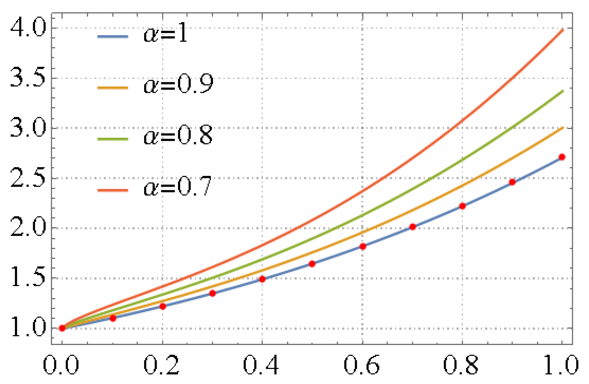
To confirm the accuracy of the recommended approach, we calculated the $R. E.$ of the LFPS approximate solution at different numbers of iterations and varied values of the fractional order derivative $\alpha$, and summarized in

Table 1. The residual errors of the LFPS solutions for Example 1.

ti	α = 0.9	α = 0.8	α = 0.7	α = 0.6
0.1	$3.05125\times {10}^{-8}$	$2.76818\times {10}^{-8}$	$1.25598\times {10}^{-7}$	$3.32936\times {10}^{-7}$
0.2	$5.44445\times {10}^{-6}$	$2.4180\times {10}^{-6}$	$2.70504\times {10}^{-5}$	$7.78659\times {10}^{-5}$
0.3	$1.15718\times {10}^{-4}$	$1.38234\times {10}^{-6}$	$6.74897\times {10}^{-4}$	$2.07896\times {10}^{-3}$
0.4	$1.03751\times {10}^{-3}$	$4.43181\times {10}^{-4}$	$7.01985\times {10}^{-3}$	$2.28483\times {10}^{-2}$

. One can observe from Table 1 that the numerical comparisons simulation reflects the accuracy of the LFPS approach. Graphically, the behavior of the attained analytic-approximate series solution of FVIDE (17) is displayed in a 2D plot as in Figure 1. It is clear from the graphical representation that the LFPS solutions in different cases of the fractional order derivative, $\alpha$, simulate the exact solution. Finally, we provided the residual error for Example 1 at different terms and times when the fixed value of FD $\alpha =0.8$. It is clear that, from the mentioned simulation in

Table 2. The residual error of the LFPS solutions at different terms and times with $\mathsf{\alpha }=0.8$ for Example 1.

	J	20	40	60	80
ti
0.1		$2.23231\times {10}^{-2}$	$6.03273\times {10}^{-4}$	$5.48087\times {10}^{-6}$	$2.76818\times {10}^{-8}$
0.2		$8.31149\times {10}^{-2}$	$7.32976\times {10}^{-3}$	$2.58114\times {10}^{-4}$	$2.4180\times {10}^{-6}$
0.3		$1.85919\times {10}^{-1}$	$3.28381\times {10}^{-2}$	$2.64048\times {10}^{-3}$	$1.38234\times {10}^{-6}$
0.4		$3.35873\times {10}^{-1}$	$9.8273\times {10}^{-2}$	$1.45347\times {10}^{-2}$	$4.43181\times {10}^{-4}$

, the values of residual errors will further decrease with increasing terms. So, the accuracy, efficiency, and convergences of the designed algorithm are confirmed.

Example 2.

Consider the following nonlinear FVIDE:

$${\mathfrak{D}}_t^{\alpha }u\left(t\right)=-2\mathit{sin}\left(t\right)-\frac{1}{3}\mathit{cos}\left(t\right)-\frac{2}{3}\mathit{cos}\left(2t\right)+{{\displaystyle \int }}_0^t\mathit{cos}\left(t-x\right)u^2\left(x\right)dx,\hspace{1em}\hspace{1em}\alpha \in \left(0,1\right],$$

(30)

Subject to the initial condition $u\left(0\right)=1$. The exact solution of (29) at $\alpha =1$ is $u\left(t\right)=\mathit{cos}\left(t\right)-\mathit{sin}\left(t\right)$ [50].

As we do in Example 1, we should first transform (30) into the new Laplace space, that is:

$${\xi }^{\alpha }U\left(\xi \right)-{\xi }^{\alpha -1}u\left(0\right)=-2\mathcal{L}\left[\mathit{sin}\left(t\right)\right]-\frac{1}{3}\mathcal{L}\left[\mathit{cos}\left(t\right)\right]-\frac{2}{3}\mathcal{L}\left[\mathit{cos}\left(2t\right)\right]+\mathcal{L}\left[\mathit{cos}\left(t\right)\right]\times \mathcal{L}\left[u^2\left(t\right)\right].$$

(31)

and the L-REF of (31) can be identified as:

$$\mathcal{L}\left\{Re{s}_U\left(\xi \right)\right\}=U\left(\xi \right)-\frac{u\left(0\right)}{\xi }-\frac{1}{{\xi }^{\gamma q}}\left(\mathcal{L}\left[\mathit{sin}\left(t\right)\right]-\frac{1}{3}\mathcal{L}\left[\mathit{cos}\left(t\right)\right]-\frac{2}{3}\mathcal{L}\left[\mathit{cos}\left(2t\right)\right]+\mathcal{L}\left[\mathit{cos}\left(t\right)\right]\times \mathcal{L}\left[u^2\left(t\right)\right]\right).$$

(32)

Write the LTs of (32) in the following FSE:

• If $qi$ is odd, then

$$\mathcal{L}\left[\mathit{sin}\left(t\right)\right]={\displaystyle \sum }_{i=0}^J\frac{a_i}{{\xi }^{qi+1}}={\displaystyle \sum }_{i=0}^J\frac{{\left(-1\right)}^{\frac{qi-1}{2}}}{{\xi }^{qi+1}},$$

(33)

• If $qi$ is even, then

$$\begin{array}{c}\mathcal{L}\left[\mathit{cos}\left(t\right)\right]={\displaystyle {\displaystyle \sum }_{i=0}^J}\frac{c_i}{{\xi }^{qi+1}}={\displaystyle {\displaystyle \sum }_{i=0}^J}\frac{{\left(-1\right)}^{\frac{qi}{2}}}{{\xi }^{qi+1}},\\ \mathcal{L}\left[\mathit{cos}\left(2t\right)\right]={\displaystyle {\displaystyle \sum }_{i=0}^J}\frac{b_i}{{\xi }^{qi+1}}={\displaystyle {\displaystyle \sum }_{i=0}^J}\frac{{\left(-1\right)}^{\frac{qi}{2}}{\left(2\right)}^{qi}}{{\xi }^{qi+1}},\end{array}$$

(34)

• The nonlinear term

$$\begin{array}{c}\mathcal{L}\left[\mathit{cos}\left(t\right)\right]\times \mathcal{L}\left[u^2\left(t\right)\right]\hfill \\ ={\displaystyle {\displaystyle \sum }_{i=0}^J}\frac{c_i}{{\xi }^{qi+1}} {\displaystyle {\displaystyle \sum }_{i=0}^{2J}}\frac{\Gamma \left(qi+1\right)}{{\xi }^{qi+1}}{\displaystyle {\displaystyle \sum }_{n=\mathit{max}\left[0,i-J\right]}^{\mathit{min}\left[J,i\right]}}\frac{u_n{u}_{i-n}}{\Gamma \left(nq+1\right)\Gamma \left(q\left(i-n\right)+1\right)}\hfill \\ ={\displaystyle {\displaystyle \sum }_{i=0}^{3J}}\frac{1}{{\xi }^{q\left(i+\frac{1}{q}\right)+1}}{\displaystyle {\displaystyle \sum }_{n=\mathit{max}\left[0,i-J\right]}^{\mathit{min}\left[i,2J\right]}}\Gamma \left(qn+1\right)c_{i-n}\hfill \\ {\displaystyle {\displaystyle \sum }_{j=\mathit{max}\left[0,i-J\right]}^{\mathit{min}\left[J,i\right]}}\frac{u_j{u}_{n-j}}{\Gamma \left(qj+1\right)\Gamma \left(q\left(n-j\right)+1\right)},\hfill \end{array}$$

(35)

Using the FSEs (9) and (33)–(35), the $j$-th L-REF of (32) can be written as:

$$\begin{array}{cc}\mathcal{L}\left\{Re{s}_{U_J}\left(\xi \right)\right\}=& {\displaystyle {\displaystyle \sum }_{i=1}^J}\frac{u_i}{{\xi }^{qi+1}}\hfill \\ & +(2{\displaystyle {\displaystyle \sum }_{i=0}^J}\frac{a_i}{{\xi }^{q\left(i+\gamma \right)+1}}+\frac{1}{3}{\displaystyle {\displaystyle \sum }_{i=0}^J}\frac{c_i}{{\xi }^{q\left(i+\gamma \right)+1}}+\frac{2}{3}{\displaystyle {\displaystyle \sum }_{i=0}^J}\frac{b_i}{{\xi }^{q\left(i+\gamma \right)+1}}\hfill \\ & -{\displaystyle {\displaystyle \sum }_{i=0}^{3J}}\frac{1}{{\xi }^{q\left(i+\frac{1}{q}+\gamma \right)+1}}{\displaystyle {\displaystyle \sum }_{n=\mathit{max}\left[0,i-J\right]}^{\mathit{min}\left[i,2J\right]}}\Gamma \left(qn+1\right)c_{i-n}\hfill \\ & {\displaystyle {\displaystyle \sum }_{j=\mathit{max}\left[0,i-J\right]}^{\mathit{min}\left[J,i\right]}}\frac{u_j{u}_{n-j}}{\Gamma \left(qj+1\right)\Gamma \left(q\left(n-j\right)+1\right)}).\hfill \end{array}$$

(36)

By solving $\underset{\xi \to \infty }{lim}{\xi }^{m\alpha +1}\mathcal{L}\left\{Re{s}_{U_J}\left(\xi \right)\right\}=0$, we have

$$\begin{array}{cc}{u}_m=-(2a_{m-\gamma }& +\frac{1}{3}{c}_{m-\gamma }+\frac{2}{3}{b}_{m-\gamma })\hfill \\ & +{\displaystyle {\displaystyle \sum }_{n=\mathit{max}\left[0,i-J\right]}^{\mathit{min}\left[m-\frac{1}{q}-\gamma ,2J\right]}}\Gamma \left(qn+1\right)c_{m-\frac{1}{q}-\gamma -n}{\displaystyle {\displaystyle \sum }_{j=\mathit{max}\left[0,i-J\right]}^{\mathit{min}\left[J,i\right]}}\frac{u_j{u}_{n-j}}{\Gamma \left(qj+1\right)\Gamma \left(q\left(n-j\right)+1\right)},\hfill \end{array}$$

(37)

for $m=\gamma ,\gamma +1,\dots ,J$, and $u_0=1,u_i=0$ for $i=1,2,\dots ,\gamma -1$.

In the case of $\alpha =0.9$, we can choose $q=\frac{1}{10},\gamma =9$. Setting $u_0=1,u_i=0,$ for $i=1,2,\dots ,8$, then the nonzero terms for $m$ from 9 to 40 are $u_9=-1,u_{19}=-1,u_{28}=-2,u_{29}=3,u_{37}=\frac{\Gamma \left(\frac{14}{5}\right)}{\Gamma {\left(\frac{19}{10}\right)}^2},u_{38}=-2,u_{39}=1$. So, the analytic-approximate solution is given by

$$u\left(t\right)=1-\frac{t^{\raisebox{1ex}{$9$}\!\left/ \!\raisebox{-1ex}{$10$}\right.}}{\Gamma \left(\frac{19}{10}\right)}-\frac{t^{\raisebox{1ex}{$19$}\!\left/ \!\raisebox{-1ex}{$10$}\right.}}{\Gamma \left(\frac{29}{10}\right)}-\frac{2t^{\raisebox{1ex}{$14$}\!\left/ \!\raisebox{-1ex}{$5$}\right.}}{\Gamma \left(\frac{19}{5}\right)}+\frac{3t^{\raisebox{1ex}{$29$}\!\left/ \!\raisebox{-1ex}{$10$}\right.}}{\Gamma \left(\frac{39}{10}\right)}+\frac{t^{\raisebox{1ex}{$37$}\!\left/ \!\raisebox{-1ex}{$10$}\right.}\Gamma \left(\frac{14}{5}\right)}{\Gamma {\left(\frac{19}{10}\right)}^2\Gamma \left(\frac{47}{10}\right)}-\frac{2t^{\raisebox{1ex}{$19$}\!\left/ \!\raisebox{-1ex}{$5$}\right.}}{\Gamma \left(\frac{24}{5}\right)}+\frac{t^{\raisebox{1ex}{$39$}\!\left/ \!\raisebox{-1ex}{$10$}\right.}}{\Gamma \left(\frac{49}{10}\right)}.$$

(38)

In the same manner, we gain $\gamma =8, 7$ for $\alpha =0.8, 0.7$, respectively.

Table 3. The residual errors of the LFPS solutions for Example 2.

ti	α = 0.9	α = 0.8	α = 0.7	α = 0.6	α = 0.5
0.1	$4.01872\times {10}^{-12}$	$1.14969\times {10}^{-10}$	$3.51448\times {10}^{-11}$	$1.2662\times {10}^{-10}$	$7.2709\times {10}^{-11}$
0.2	$8.73393\times {10}^{-10}$	$3.65742\times {10}^{-8}$	$1.19959\times {10}^{-8}$	$3.75249\times {10}^{-8}$	$2.55736\times {10}^{-8}$
0.3	$1.60784\times {10}^{-8}$	$1.06161\times {10}^{-6}$	$3.56381\times {10}^{-7}$	$9.78584\times {10}^{-7}$	$6.88552\times {10}^{-7}$
0.4	$8.94261\times {10}^{-8}$	$1.15723\times {10}^{-5}$	$3.91616\times {10}^{-6}$	$9.47861\times {10}^{-6}$	$6.18322\times {10}^{-6}$
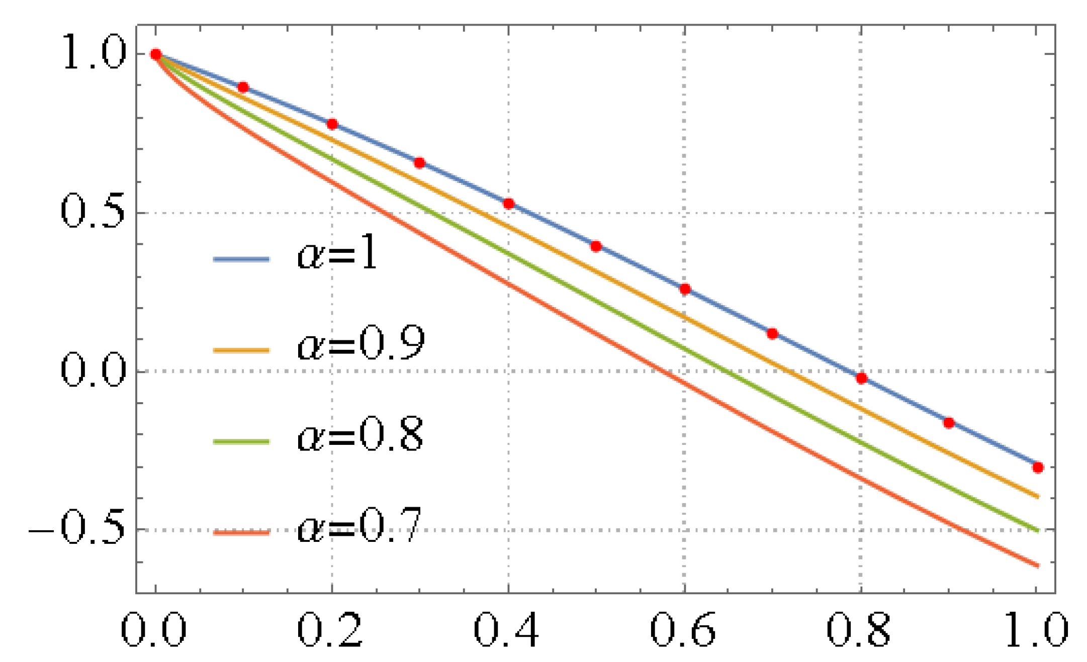
0.5	$9.02043\times {10}^{-8}$	$7.37875\times {10}^{-5}$	$2.49509\times {10}^{-5}$	$5.35762\times {10}^{-5}$	$2.78115\times {10}^{-5}$

compares the residual errors for gained LFPS approximate solutions to FVIDE (29) at varied values of $\alpha$. From Table 3, it is obvious that the effect of the FD parameter on the values of residual errors will further decrease over the domain of interest of obtained solutions and this confirms the accuracy of our proposed method. Figure 2 displays the 2D plot of the exact and the LFPS solutions for Example 2 when $\alpha \in \left\{0.7,0.8,0.9,1.0\right\}$ in the domain $t\in \left[0, 1\right]$. This graphical representation indicates that the solutions attained via the recommended algorithm converge to the exact solution when $\alpha$ tends to 1, and these solutions overlap at $\alpha =1$. Finally, in

Table 4. The residual error of the LFPS solutions at different terms and times with $\mathsf{\alpha }=0.8$ for Example 2.

	J	20	40	60	80
ti
0.1		$3.23928\times {10}^{-3}$	$4.56363\times {10}^{-5}$	$3.98756\times {10}^{-7}$	$2.06271\times {10}^{-9}$
0.2		$1.81809\times {10}^{-3}$	$5.3666\times {10}^{-4}$	$1.43983\times {10}^{-5}$	$3.32608\times {10}^{-7}$
0.3		$1.00238\times {10}^{-2}$	$2.20152\times {10}^{-3}$	$1.13732\times {10}^{-4}$	$6.45179\times {10}^{-6}$
0.4		$3.55286\times {10}^{-2}$	$5.84874\times {10}^{-3}$	$4.83321\times {10}^{-4}$	$5.2582\times {10}^{-5}$

we provided the residual errors for the results attained from Example 2 at different terms and times when the FD was fixed at $\alpha =0.8$ to demonstrate the convergence of the proposed method. From this table, one notices that the values of residual errors will further decrease with increasing terms of obtained solutions, and this proves the accuracy, efficiency, and convergence of the LFPS scheme.

5. Conclusions

In this article, a modified LFPS algorithm has been profitably implemented to explore the analytic-approximate solution of nonlinear FVIDEs involving the Caputo-FD of order $\alpha : 0<\alpha \le 1$, with fitting ICs. The essence and procedure of our recommended algorithm is the construction of the solutions via solving studied equations using the LT principle and simulating the FPS approach in the Laplace space. In the stage of finding out the unknowns of the suggested solution by performing minimal calculations, the recommended algorithm needs an infinite limit concept and not a FD, as in FPS. In comparison, the procedure of FPS needs $\left(n-1\right)$-Caputo FD of the residual function, which may take time in the stages of exploring the solution. The accuracy and effectiveness of the LFPS algorithm are clarified by graphical and numerical simulations of the results. The impact of the Caputo-FD order can be observed in the behaviors of LFPS-curves for various values of $\alpha$. Analysis of acquired results declares that the recommended algorithm is considered to be a convenient, reliable computational algorithm to treat wide aspects of nonlinear fractional models with high accuracy. Conclusively, providing analytic-approximate solutions for various fractional IDEs and IDEs is a difficult undertaking. In future studies, we plan to investigate solutions of these models via the modified LFPS method under Caputo-FD of the order of a positive irrational number.

References

1. Loverro, A. Fractional Calculus: History, Definitions and Applications for the Engineer; Rapport Technique; University of Notre Dame, Department of Aerospace and Mechanical Engineering: Notre Dame, IN, USA, 2004. [Google Scholar]
2. Mainardi, F. Fractional Calculus and Waves in Linear Viscoelasticity: An Introduction to Mathematical Models; World Scientific: Singapore, 2022. [Google Scholar]
3. Yang, X.J. General Fractional Derivatives: Theory, Methods and Applications; CRC Press: Boca Raton, FL, USA, 2019. [Google Scholar]
4. Kilbas, A.A.; Srivastava, H.M.; Trujillo, J.J. Theory and Applications of Fractional Differential Equations; Elsevier: Amsterdam, The Netherlands, 2006; p. 204. [Google Scholar]
5. Inc, M.; Yusuf, A.; Aliyu, A.I.; Baleanu, D. Soliton solutions and stability analysis for some conformable nonlinear partial differential equations in mathematical physics. Opt. Quantum Electron. 2018, 50, 190. [Google Scholar] [CrossRef]
6. Akdemir, A.O.; Dutta, H.; Atangana, A. Fractional Order Analysis: Theory, Methods and Applications; John Wiley & Sons: Hoboken, NJ, USA, 2020. [Google Scholar]
7. Bagley, R.L.; Torvik, P.J. Fractional calculus in the transient analysis of viscoelastically damped structures. AIAA J. 1985, 23, 918–925. [Google Scholar] [CrossRef]
8. Al-Smadi, M.; Djeddi, N.; Momani, S.; Al-Omari, S.; Araci, S. An attractive numerical algorithm for solving nonlinear Caputo–Fabrizio fractional Abel differential equation in a Hilbert space. Adv. Differ. Equ. 2021, 2021, 271. [Google Scholar] [CrossRef]
9. Ragb, O.; Wazwaz, A.M.; Mohamed, M.; Matbuly, M.S.; Salah, M. Fractional differential quadrature techniques for fractional order Cauchy reaction-diffusion equations. Math. Methods Appl. Sci. 2023, 46, 10216–10233. [Google Scholar] [CrossRef]
10. Hashim, I.; Sharadga, M.; Syam, M.I.; Al-Refai, M. A Reliable Approach for Solving Delay Fractional Differential Equations. Fractal Fract. 2022, 6, 124. [Google Scholar] [CrossRef]
11. Povstenko, Y. Linear Fractional Diffusion-Wave Equation for Scientists and Engineers; Birkhäuser: New York, NY, USA, 2015. [Google Scholar]
12. Syam, M.; Al-Refai, M. First order delay equations Implicit hybrid method. Alex. Eng. J. 2020, 59, 2677–2681. [Google Scholar] [CrossRef]
13. Lopes, A.M.; Machado, J.A.T.; Pinto, C.M.A.; Galhano, A.M.S.F. Fractional dynamics and MDS visualization of earthquake phenomena. Comput. Math. Appl. 2013, 66, 647–658. [Google Scholar] [CrossRef] [Green Version]
14. Hengamian Asl, E.; Saberi-Nadjafi, J.; Gachpazan, M. Numerical Solution of Fractional-Order Population Growth Model Using Fractional-Order Muntz–Legender Collocation Method and Pade–Approximations. Jordan J. Math. Stat. 2022, 15, 157–175. [Google Scholar]
15. Hartley, T.T.; Lorenzo, C.F.; Killory Qammer, H. Chaos in a fractional order Chua’s system. IEEE Trans. Circuits Syst. I Fundam. Theory Appl. 1995, 42, 485–490. [Google Scholar] [CrossRef]
16. Oldham, K.B. The reformulation of an infinite sum via semiintegration. SIAM J. Math. Anal. 1983, 14, 974–981. [Google Scholar] [CrossRef]
17. Povstenko, Y.Z. Thermoelasticity that uses fractional heat conduction equation. J. Math. Sci. 2009, 162, 296–305. [Google Scholar] [CrossRef]
18. Baskin, E.; Iomin, A. Electro-chemical manifestation of nanoplasmonics in fractal media. Cent. Eur. J. Phys. 2013, 11, 676–684. [Google Scholar] [CrossRef] [Green Version]
19. Bapna, I.B.; Mathur, N. Application of fractional calculus in statistics. Int. J. Contemp. Math. Sci. 2012, 7, 849–856. [Google Scholar]
20. Goncalves, E.; Zeidan, D. Numerical simulation of unsteady cavitation in liquid hydrogen flows. J. Eng. Syst. Model. Simul. 2017, 9, 41–51. [Google Scholar] [CrossRef]
21. Kulish, V.V.; Lage, J.L. Application of fractional calculus to fluid mechanics. J. Fluids Eng. 2002, 124, 803–806. [Google Scholar] [CrossRef]
22. Derdar, N. Nonlinear Implicit Caputo-Hadamard Fractional Differential Equation with Fractional Boundary Conditions. Jordan J. Math. Stat. JJMS 2022, 15, 999–1014. [Google Scholar]
23. Bendouma, B. Monotone Iterative Technique for a Coupled System of Nonlinear Conformable Fractional Dynamic Equations on Time Scales. Jordan J. Math. Stat. JJMS 2023, 16, 41–55. [Google Scholar]
24. Al-Smadi, M.; Al-Omari, S.; Karaca, Y.; Momani, S. Effective Analytical Computational Technique for Conformable Time-Fractional Nonlinear Gardner Equation and Cahn-Hilliard Equations of Fourth and Sixth Order Emerging in Dispersive Media. J. Funct. Spaces 2022, 2022, 4422186. [Google Scholar] [CrossRef]
25. Alaroud, M.; Alomari, A.-K.; Tahat, N.; Al-Omari, S.; Ishak, A. A Novel Solution Approach for Time-Fractional Hyperbolic Telegraph Differential Equation with Caputo Time Differentiation. Mathematics 2023, 11, 2181. [Google Scholar] [CrossRef]
26. Alaroud, M.; Al-Smadi, M.; Rozita Ahmad, R.; Salma Din, U.K. An Analytical Numerical Method for Solving Fuzzy Fractional Volterra Integro-Differential Equations. Symmetry 2019, 11, 205. [Google Scholar] [CrossRef] [Green Version]
27. Ma, C. A Novel Computational Technique for Impulsive Fractional Differential Equations. Symmetry 2019, 11, 216. [Google Scholar] [CrossRef] [Green Version]
28. Mahmood, S.; Shah, R.; Khan, H.; Arif, M. Laplace Adomian Decomposition Method for Multi Dimensional Time Fractional Model of Navier-Stokes Equation. Symmetry 2019, 11, 149. [Google Scholar] [CrossRef] [Green Version]
29. Youbi, F.; Momani, S.; Hasan, S.; Al-Smadi, M. Effective numerical technique for nonlinear Caputo-Fabrizio systems of fractional Volterra integro-differential equations in Hilbert space. Alex. Eng. J. 2022, 61, 1778–1786. [Google Scholar] [CrossRef]
30. Zedan, H.A.; Alaidarous, E. Haar wavelet method for the system of integral equations. Abstr. Appl. Anal. 2014, 2014, 418909. [Google Scholar] [CrossRef]
31. Biazar, J. Solution of systems of integral-differential equations by Adomian decomposition method. Appl. Math. Comput. 2005, 168, 1232–1238. [Google Scholar] [CrossRef]
32. Abbasbandy, S.; Hashemi, M.S.; Hashim, I. On convergence of homotopy analysis method and its application to fractional integro-differential equations. Quaest. Math. 2013, 36, 93–105. [Google Scholar] [CrossRef]
33. Baleanu, D.; Zibaei, S.; Namjoo, M.; Jajarmi, A. A nonstandard finite difference scheme for the modeling and non-identical synchronization of a novel fractional chaotic system. Adv. Differ. Equ. 2021, 2021, 308. [Google Scholar] [CrossRef]
34. Maleknejad, K.; Aghazadeh, N.; Rabbani, M. Numerical solution of second kind Fredholm integral equations system by using a Taylor-series expansion method. Appl. Math. Comput. 2006, 175, 1229–1234. [Google Scholar] [CrossRef]
35. Sahin, N.; Yuzbasi, S.; Gulsu, M. A collocation approach for solving systems of linear Volterra integral equations with variable coefficients. Comput. Math. Appl. 2011, 62, 755–769. [Google Scholar] [CrossRef] [Green Version]
36. Liaqat, M.I.; Khan, A.; Alam, M.; Pandit, M.K. A highly accurate technique to obtain exact solutions to time-fractional quantum mechanics problems with zero and nonzero trapping potential. J. Math. 2022, 2022, 9999070. [Google Scholar] [CrossRef]
37. Alshammari, M.; Al-Smadi, M.; Arqub, O.A.; Hashim, I.; Alias, M.A. Residual Series Representation Algorithm for Solving Fuzzy Duffing Oscillator Equations. Symmetry 2020, 12, 572. [Google Scholar] [CrossRef] [Green Version]
38. Aljarrah, H.; Alaroud, M.; Ishak, A.; Darus, M. Adaptation of Residual-Error Series Algorithm to Handle Fractional System of Partial Differential Equations. Mathematics 2021, 9, 2868. [Google Scholar] [CrossRef]
39. Zhang, Y.; Kumar, A.; Kumar, S.; Baleanu, D.; Yang, X. Residual power series method for time-fractional Schrödinger equations. J. Nonlinear Sci. Appl. 2016, 9, 5821–5829. [Google Scholar] [CrossRef]
40. Tariq, H.; Akram, G. Residual power series method for solving time-space-fractional Benney–Lin equation arising in falling film problems. J. Appl. Math. Comput. 2017, 55, 683–708. [Google Scholar] [CrossRef]
41. Kumar, A.; Kumar, S.; Singh, M. Residual power series method for fractional Sharma-Tasso-Olever equation. Commun. Numer. Anal. 2016, 1, 1–10. [Google Scholar] [CrossRef]
42. El-Ajou, A. Adapting the Laplace transform to create solitary solutions for the nonlinear time-fractional dispersive PDEs via a new approach. Eur. Phys. J. Plus 2021, 136, 229. [Google Scholar] [CrossRef]
43. Alaroud, M.; Tahat, N.; Al-Omari, S.; Suthar, D.L.; Gulyaz-Ozyurt, S. An Attractive Approach Associated with Transform Functions for Solving Certain Fractional Swift-Hohenberg Equation. J. Funct. Spaces 2021, 2021, 3230272. [Google Scholar] [CrossRef]
44. Liaqat, M.I.; Okyere, E. Comparative Analysis of the Time-Fractional Black–Scholes Option Pricing Equations (BSOPE) by the Laplace Residual Power Series Method (LRPSM). J. Math. 2023, 2023, 6092283. [Google Scholar] [CrossRef]
45. Aljarrah, H.; Alaroud, M.; Ishak, A.; Darus, M. Approximate Solution of Nonlinear Time-Fractional PDEs by Laplace Residual Power Series Method. Mathematics 2022, 10, 1980. [Google Scholar] [CrossRef]
46. Alaroud, M.; Ababneh, O.; Tahat, N.; Al-Omari, S. Analytic technique for solving temporal time-fractional gas dynamics equations with Caputo fractional derivative. AIMS Math. 2022, 7, 17647–17669. [Google Scholar] [CrossRef]
47. Alaroud, M.; Alomari, A.-K.; Tahat, N.; Ishak, A. Analytical Computational Scheme for Multivariate Nonlinear Time-Fractional Generalized Biological Population Model. Fractal Fract. 2023, 7, 176. [Google Scholar] [CrossRef]
48. Oqielat, M.A.N.; Eriqat, T.; Al-Zhour, Z.; Ogilat, O.; El-Ajou, A.; Hashim, I. Construction of fractional series solutions to nonlinear fractional reaction–diffusion for bacteria growth model via Laplace residual power series method. Int. J. Dyn. Control 2023, 11, 520–527. [Google Scholar] [CrossRef]
49. Moa’ath, N.O.; El-Ajou, A.; Al-Zhour, Z.; Eriqat, T.; Al-Smadi, M. A new approach to solving fuzzy quadratic Riccati differential equations. Int. J. Fuzzy Log. Intell. Syst. 2022, 22, 23–47. [Google Scholar]
50. Wazwaz, A.M. The combined Laplace transform—Adomian decomposition method for handling nonlinear Volterra integro–differential equations. Appl. Math. Comput. 2010, 216, 1304–1309. [Google Scholar] [CrossRef]
Figure 1. 2D plots of fractional curves of the LFPS approximate solution for Example 1, at various values of α , versus the exact solution Symmetry 15 01296 i001.
Symmetry 15 01296 g001
Figure 2. 2D plots of fractional curves of the LFPS approximate solution for Example 2 at various values of α , versus the exact solution Symmetry 15 01296 i002.
Symmetry 15 01296 g002