
Scaling Symmetries and Parameter Reduction in Epidemic SI(R)S Models

Department of Physics, Free University Berlin, Arnimallee 14, 14195 Berlin, Germany
Symmetry 2023, 15(7), 1390; https://doi.org/10.3390/sym15071390
Submission received: 26 May 2023
/
Revised: 10 June 2023
/
Accepted: 15 June 2023
/
Published: 10 July 2023
(This article belongs to the Section Mathematics)
Abstract
:Symmetry concepts in parametrized dynamical systems may reduce the number of external parameters by a suitable normalization prescription. If, under the action of a symmetry group , parameter space becomes a (locally) trivial principal bundle, , then the normalized dynamics only depends on the quotient . In this way, the dynamics of fractional variables in homogeneous epidemic SI(R)S models, with standard incidence, absence of R-susceptibility and compartment independent birth and death rates, turns out to be isomorphic to (a marginally extended version of) Hethcote’s classic endemic model, first presented in 1973. The paper studies a 10-parameter master model with constant and I-linear vaccination rates, vertical transmission and a vaccination rate for susceptible newborns. As recently shown by the author, all demographic parameters are redundant. After adjusting time scale, the remaining 5-parameter model admits a 3-dimensional abelian scaling symmetry. By normalization we end up with Hethcote’s extended 2-parameter model. Thus, in view of symmetry concepts, reproving theorems on endemic bifurcation and stability in such models becomes needless.
Keywords:
symmetries in parametric dynamical systems; SIRS model; classic endemic model; parameter reduction; normalizationMSC:
34C23; 34C26; 37C25; 92D301. Introduction
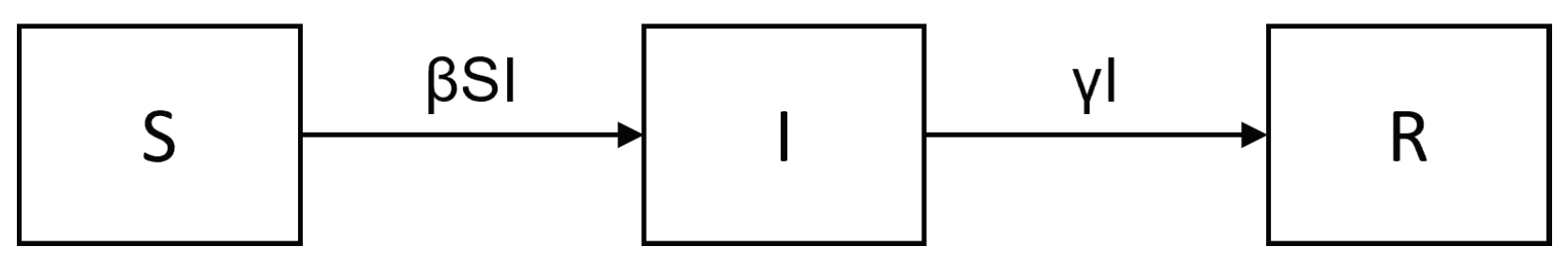
The classic SIR model was introduced by Kermack and McKendrick in 1927 [1] as one of the first models in mathematical epidemiology. The model divides a population into three compartments with fractional sizes S (Susceptible), I (Infectious) and R (Recovered), such that . The flow diagram between compartments, as given in Figure 1, leads to the dynamical system
Here, denotes the recovery rate and the effective contact rate (i.e., the number of contacts/time leading to infection of a susceptible, given the contacted was infectious). Members of R are supposed to be immune forever. Due to (1), S decreases monotonically, eventually causing and . At the end, the disease dies out, , and one maintains a nonzero final size , thus providing a model for herd immunity.
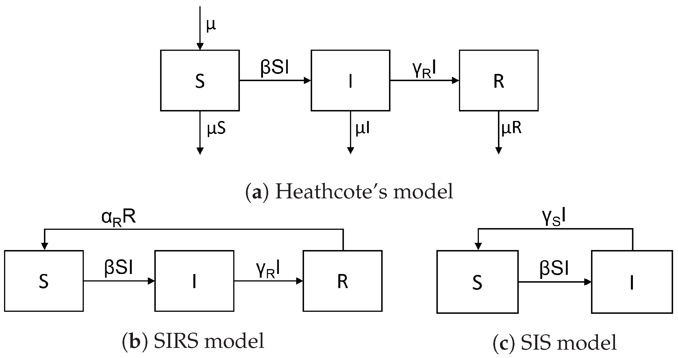
To construct models also featuring endemic situations, one needs a sufficient supply of susceptibles to keep the incidence ongoing above a positive threshold. The literature discusses three basic methods to achieve this—see Figure 2.
- The SIRS model adds an immunity waning flow, from R to S, to the SIR model, leading to the same result, with
- The SIS model considers recovery without immunity, i.e., a recovery flow from I to S, while putting . Again, this leads to the same result, with .
Since the original work by Hethcote the literature on endemic bifurcation in SI(R)S-type models is vast. For a comprehensive and self-contained overview of the history, methods and results in mathematical epidemiology see the textbook by M. Martcheva [6], wherein an extensive list of references to original papers is also given.
Of course, since 2020, there has also been a huge tsunami of papers analyzing applications of such models to COVID-19. Presenting a representative list of references at this point would overkill the scope of this paper. Some relevant references to SIRS models have been presented by the author in [7], where it has been shown that endemic oscillations predicted by the SIRS model decay much too fast to explain COVID-19 waves in the real world. More generally, one should always be aware that autonomous models with constant parameters often fail to describe time dependent social behavior due to public information, governmental measures and seasonal effects. Finally, one should also mention that SIR-type models always neglect incubation times, so this paper will not look at SEIR models addressing that.
This paper is based on the idea that, when adding more parameters to standard models, reproving theorems may become superfluous if instead there is a symmetry operation “turning parameter space north”, i.e., mapping the seemingly more complicated model to the simpler one. Obvious examples would be diagonalizing the matrix in a linear system or rotating a constant external (say magnetic) force field in a system of radially interacting particles such that . In SI(R)S-type models the simplest example has been proposed in [8], showing that, under quite general conditions, demographic parameters are explicitly redundant when looking at fractional variables (so this may be viewed as a translation symmetry in parameter space). Applying this, for example, to a recent paper on backward bifurcation in a variable population SIRS model with R-susceptibility by [9], many results of that paper already follow from earlier results in [10,11].
Going one step ahead, this paper analyzes parameter symmetries in a homogeneous 10-parameter SI(R)S ≡ combined SIRS/SIS model with standard incidence, four demographic parameters and a continuous vaccination flow from S to R. Motivated by common observations in the COVID-19 pandemic, the vaccination rate is also assumed to contain a part proportional to I. This models diminishing willingness to get vaccinated when public data indicate decreasing prevalence. For models letting the vaccination activity be functionally dependent on the history of prevalence see e.g., [12,13,14].
Using redundancy of birth and death rates and three scaling transformations, we will see that such an elaborated model in fact still boils down to a marginally extended version of Hethcote’s classic endemic model. This generalizes earlier results in [7]. As a particular consequence, an I-linear vaccination rate may always be transformed to zero. In summary, by symmetry arguments, reproving theorems on endemic bifurcation and stability in such models becomes needless.
The plan of this paper is as follows. Section 2 gives a self contained review on Hethcote’s endemic model, thereby introducing basic terminology and notation. To prepare the setting for symmetry operations, a slightly extended version will be considered by allowing also negative values of S and possibly negative recovery rates . Standard techniques for proving endemic bifurcation and stability immediately generalize to this setting. Identifying as a pure time scale, this model essentially depends on just two parameters.
Section 3 introduces the 10-parameter SI(R)S model. After removing redundant demographic parameters and performing two more transformation steps, we will see that for a wide range of parameters , including all epidemiologically interesting scenarios, this model actually becomes isomorphic to the extended 2-parameter Hethcote model. In absence of immunity waning and constant vaccination, but still with an I-linear vaccination and two recovery flows from I to R and S, respectively, the model even becomes isomorphic to the classic SIR model, see Section 3.5.
Section 4 provides a group theoretical approach to explain this scenario. There is a coordinate free concept of parameter symmetry as a group acting on phase × parameter space, , projecting to an action of on , and leaving the dynamical system form invariant. In our SI(R)S model, choosing suitable coordinates in , the group is easily identified as a composition of scaling transformations of, respectively, and , x being the replacement number. The action of on leaves the above sub-range invariant and turns into a principal -bundle. Moreover, as trivial principal bundles, and any such trivialization induces an isomorphism mapping the original system with parameter space to an equivalent system with reduced parameter space . In this way, the 2-parameter space of the extended Hethcote model is identified as the quotient . We also have a “gauge fixing result” result, showing that any parameter configuration is -equivalent to a configuration , where denotes the subset of epidemiologically admissible parameters.
Appendix A relates the Korobeinikov-Wake SIRS model in [15] to the present formulation in Section 3, showing that without additional parameter constraints their model may possibly lead to non-physical equilibrium states, . Appendix B provides a Hamiltonian approach to the ”quasi-SIR case" in Section 3.5 and Appendix C shortly describes the exceptional case of a SIS model with I-linear vaccination not covered within the main setting.
2. Hethcote’s Endemic Model Revisited
In this Section we introduce notation and terminology and shortly review Hethcote’s classic results [2,3,4,5]. Replacing , Hethcote’s model in Figure 2 leads to the dynamic system
Introducing dimensionless variables
we obtain
Here, is the basic reproduction number (also called contact number by Hethcote), i.e., the average number of new cases produced by one infected in a totally susceptible population, and x is the effective reproduction number (also called replacement number by Hethcote), i.e., the average number of new cases produced by one infected at time t. More generally, the replacement number x could be defined as the ratio inflow/outflow at the I-compartment, making the second equation in (3) universal by definition. In particular, endemic equilibria always satisfy . Looking at the domains of the definition, Equation (2) implies that
Also, only sets the time scale, i.e., without loss, one could choose and use as a rescaled time variable. We now slightly extend the above restrictions by using the following definition:
Definition 1.
By the extended Hethcote model we mean the dynamical system (3) on phase space with parameters .
Note that the limit yields the classic SIR model. Hethcote’s original methods now immediately apply to this extended definition. First note:
Lemma 1.
For any initial condition the forward flow of the system (3) stays bounded.
Proof.
Let and and denote the triangle with corners , and . Since given we can always choose as above such that , it is enough to show that is forward invariant. Since and we are left to show that on the diagonal we have . Assuming we get . If instead , then . □
Next, using as a Dulac function as in [3,4], one immediately checks , and so, by the Bendixson–Dulac theorem, in there exist no periodic solutions, homoclinic loops or oriented phase polygons of the dynamical system (3). Thus, we arrive at
Theorem 1
Proof.
Existence of for all follows from boundedness. If , then (3) can immediately be integrated yielding . If , then the disease free equilibrium is the only equilibrium point (EP) in and the statement follows by absence of periodic solutions and the Poincaré-Bendixson Theorem. If , then there also exists the endemic EP and, by the same argument, the omega limit set of must consist of one of the two EPs. If it must be , either by arguing that is a saddle point with attractive line (calculate the Jacobian), or by using that
provides a Lyapunov function satisfying , and
□
To study the asymptotic behavior at these equilibria one has to compute eigenvalues and slopes of eigenvectors of the Jacobian. For example, as already noted by Hethcote in [3,4,5], see also chapter 3.4–3.5 in the text book by M. Martcheva [6], there is a sub-range and , where the endemic equilibrium becomes spiral and hence this model shows endemic oscillations. A complete detailed analysis of possible asymptotic scenarios has also been given in [7].
3. The 10-Parameter SI(R)S Model
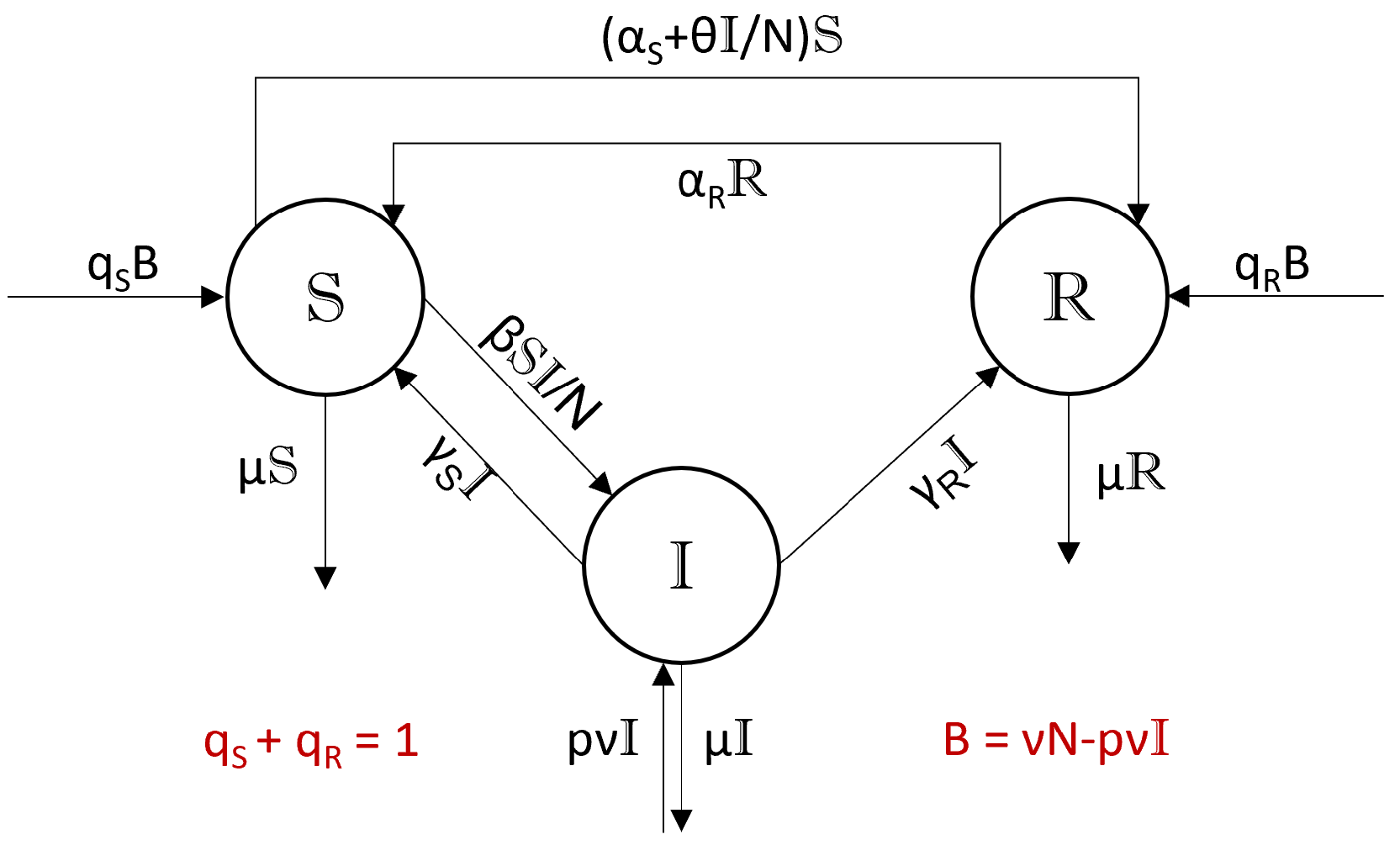
This section introduces a homogeneous 10-parameter SI(R)S-model (i.e., mixed SIRS/ SIS model) with standard incidence and flow diagram as depicted in Figure 3. The model describes the infection dynamics of three compartments with populations and total population . Members of are infectious, members of are susceptible (not immune) and members of are immune due to recovery or vaccination. To model widely experienced social behavior, Figure 3 introduces the parameter to the classic setting. It describes the willingness to get vaccinated by assuming a vaccination rate proportional to the prevalence . As we will see, such an extended model can always be transformed to the standard case (Corollary 2).
Parameters in this model are
| : | Constant vaccination rate. | |
| : | Willingness to get vaccinated given the actual prevalence . | |
| : | Immunity waning rate. | |
| : | Effective contact rate of a susceptible from . | |
| : | Recovery rates for and , respectively. . | |
| : | Mortality rate, assumed to be compartment independent. | |
| : | Rate of newborns, assumed to be compartment independent. | |
| Newborns from and are not supposed to be infected. | ||
| p | : | Probability of a newborn from to be infected. |
| B | : | Sum of not infected newborns, . |
| : | Split ratio of not infected newborns landing in and , . So, is the vaccinated portion of not infected newborns. |
Epidemiologically, all parameters are assumed nonnegative. Also, , , and . So, in total we have 10 parameters, four of which, , are purely demographic. Subcases of this model with constant population and have been analyzed e.g., in [15,16]. Of course, Hethcote’s classic endemic model is also a special subcase, which has been reinvented several times; see, e.g., [17,18,19].
At this place one should mention that there are various models in the literature treating vaccination and loss of immunity differently. For example, one might introduce a separate compartment V to distinguish vaccinated from recovered individuals (see, e.g., [20]). A model for booster vaccination with a separate compartment for primary vaccination has been proposed by [21] and periodic pulse vaccination has been studied e.g., in [22,23,24]. Time dependent vaccination rates have also been studied in [25] by applying optimal control methods and in [12] by letting the vaccination activity be functionally dependent on the history of the prevalence via the Preisach hysteresis operator. Following a similar philosophy, in [13,14] the authors use an information variable, M, to model how information on current and past states of the disease influences decisions in families whether to vaccinate or not their children.
Partial and/or waning immunity may also be modeled by introducing a diminished transmission rate directly from R to I (or V to I). Such models are well known to lead to a so-called backward bifurcation; see, e.g., [9,10,20,26,27,28]. In fact, the methods of this paper will generalize to such a setting; see [29].
The next section will show that the full 10-parameter model in Figure 3 in fact boils down to the extended Hethcote model as defined in Definition 1.
3.1. Redundancy of Birth and Death Rates
In a first step, we follow the strategy of [8], showing that in the dynamics of fractional variables the four demographic parameters become redundant. We have and
Now, demographic parameters become redundant by putting , i.e.,
In this way, the number of effective parameters reduces from ten to six. So, from now on, we put without loss and omit the tilde above parameters. Again, it is convenient to introduce dimensionless parameters. Put and
Note that . The new notation indicates a possible generalization to models where also R is susceptible [29]. With this notation the dynamics takes the form
We start with an extended parameter space by putting , and requiring . Here we put
while is understood throughout. So, denotes the epidemiologically admissible subset of parameters. Also, we start with defining the system (8) on the extended phase space given by the half plane
Clearly, stays invariant under the dynamics (8) for all . Epidemiologically the system is considered for initial conditions in the physical triangle
It is straightforward to check that for all this triangle stays forward invariant under the dynamics (8), i.e., if and then . (More generally, it can be shown that is forward invariant, iff .)
Remark 1.
The “quasi-SIR limit” becomes an integrable Hamiltonian model, see Section 3.5 and Appendix B.
3.2. Dynamics of the Replacement Number
From now on, we substitute and drop the variable R. Hence and . In a second step, we proceed in a similar way to [7] and define
Then and the equations of motion (8) are equivalent to
Here, x is again the replacement number and is the well known vaccination reduced reproduction number [30]. Note that for the definitions imply and . Also note that choosing the variables has further reduced the number of free parameters from six to four, i.e., the dynamics in Equation (16) is independent of and . Instead, these parameters now fix the image of the physical triangle in -space.
So, given and the position of , one recovers . More precisely, we have
Lemma 2.
Put and . The map
is bijective with inverse given by
Moreover,
Proof.
Lemma 2 motivates the following definition.
Definition 2.
Let , and be given. Then , respectively triangles , are called admissible, if .
Since for physical triangles are forward invariant under the dynamics (8), we conclude
Corollary 1.
Admissible triangles are forward invariant under the dynamics (16).
Remark 2.
One should remark that Equation (16) has been obtain in equivalent form by Korobeinikov and Wake in [15], with , but without the upper bound . This is due to the fact that the authors consider possibly unbalanced birth and death rates, , but still require the total population to be time independent. In other words, the recovered/immune compartment is forced to obey . For , this leads to a non-constant and S- and I-dependent mortality rate in the R-compartment. Nevertheless, this system transforms to the present setting, with , but possibly with and negative, so , see Appendix A for the details. The fact that global stability results as in [15] may also hold outside of will be covered by Theorem 2 below.
3.3. Equilibrium States
From the dynamics (16) we immediately read off the solutions of , yielding a disease free equilibrium and an endemic equilibrium ,
where the endemic equilibrium requires and . In terms of original variables and parameters, this results in
This generalizes well known results in the literature [2,3,4,5,15,16,17,18,19] to the case of our present 10-parameter model.
Remark 3.
As already noted, for we have , where the boundary case is equivalent to . In particular, it also requires and . Epidemiologically, this case is uninteresting and excluded in what follows. It will be discussed shortly in Appendix C.
Remark 4.
Typically, vaccination diminishes the reproduction number as in Equation (15), where . This allows us quite generally to determine lower bounds on vaccination rates to achieve herd immunity by requiring , see e.g. the text book [6]. In contrast, here is independent of the I-linear vaccination rate . In fact, just diminishes , see (22), and increases the recovered/immune fraction accordingly. But it doesn’t influence the value of , nor the disease free equilibrium, nor the endemic threshold . In fact, as we will see in Corollary 2 in Section 4.2, by a scaling transformation , , the SI(R)S model (8) with parameters in and maps isomorphically to a system with appropriately transformed parameters , i.e., , while keeping invariant.
3.4. Transformation to the Extended Hethcote Model
In the third step, we now apply a rescaling transformation of as first introduced in [7]. This will show that for the system (16) is isomorphic to an extended Hethcote model as defined in Definition 1. Hence, to prove stability properties for the above SI(R)S model equilibria, we just need to quote Hethcote’s results in the formulation of Theorem 1.
Proposition 1
Proof.
By straightforward calculation. □
Since and , the results of Theorem 1 now immediately translate to our original model. In doing so, due to the global boundedness property in Lemma 1, we no longer have to restrict ourselves to parameter constraints to guarantee the forward invariance of physical triangles. The following more general definition of will suffice.
Theorem 2.
- (i)
- For any initial conditon the forward orbit exists for all . If or , then Otherwise
- (ii)
- If then .
- (iii)
- If and , then .
3.5. The Quasi SIR Limit
In the limit , and the system (8) becomes a combined SIR/SIS model with absence of immunity waning and just an I-linear vaccination rate. In this case, we obtain and . For this is the pure SIS model, , and for the transformation (23) reduces to the classic SIR model, Equation (24) with . Hence, this model also shows herd immunity and standard results for the classic SIR model [1,3,4,31,32,33] now apply, see Appendix B for more details. Below, let denote the upper branch of the so-called Lambert-W function [34,35], i.e., the inverse of .
Theorem 3.
Consider the SI(R)S model (8) for , and , excluding the case (pure SIS model). Assume and initial conditions , and .
- (i)
- The limits exist and satisfy
- (ii)
- Put and . Then the following generalized final size formula holds
- (iii)
- Assume . As a fraction of the total increase in the R-compartment is vaccinated.
Remark 5.
Note that is not backward invariant, i.e., depending on one may obtain . Also note that the case reduces to the classic SIR model for variables , equipped with an I-linear vaccination rate . In this case, the final size (27) is independent of . In fact, under the usual assumption , it reduces to the standard final size formula in the classic SIR model; see, e.g., [1,3,5,31,36,37,38]. Theorem 3 is proven in Appendix B, where also the cases and are discussed.
In summary, in this section we have seen that, for parameters (25), the SI(R)S model (8) is isomorphic to the extended Hethcote model (24), and that in the limit and we obtain a quasi-SIR model. The equivalences of these models have been obtained by applying three scaling transformations
The next section studies these transformations and the relation between and more systematically under group theoretical aspects.
4. Symmetries and Parameter Reduction
4.1. Basic Concepts
For simplicity, unless stated explicitly, all maps in this section are supposed to be . A model class on some phase space is a family of dynamical systems , where are vector fields on parametrized by a set of external parameters . Typically and for we have , where , , are linearly independent as vector fields on . Given a model class , it is helpful to consider also as dynamical variables obeying . Putting , the associated vector field is given by .
Two model classes and are said to be isomorphic, if there exists a diffeomorphism projecting to a diffeomorphism (i.e., ), such that . Here, denotes the canonical projection and, for diffeomorphisms , denotes the “push forward” on vector fields, .
Definition 3.
A parameter symmetry group of a model class is a left -action on by diffeomorphisms , , projecting to a -action on , denoted by , such that for all .
To understand this definition, let . Then and acts as a parameter symmetry group, iff for all and
In other words, the equations of motion stay invariant under the transformation , if we transform parameters accordingly. Also note that in most common examples the -action on factorizes, i.e., is independent of and .
Given a parameter symmetry , the family of parametrized dynamical systems falls into isomorphy classes labeled by the orbits . Under some technical assumptions, this allows us to construct equivalent transformed systems with reduced parameter space . Equivalently, one may “turn parameter space north” by choosing a suitable section and solving the system for . A simple example would be , , the space of symmetric -matrices, and . In this case parameter reduction means diagonalizing . Another example would be the dynamics of mutually interacting classical particles in a constant external (say magnetic) field . In this case and and “turning parameter space north” means putting without loss . As a third example, quasimonomial transformations to canonical forms for generalized Lotka–Volterra (GLV) systems can also be understood in this way; see [39,40].
4.2. The SI(R)S Symmetry
We now apply this formalism to the 6-parameter SI(R)S model (8) with phase space and parameter space , where is given in Equation (10). Following the three scaling transformations in (28), denote the multiplicative abelian group
Elements of are denoted . By convenient notation, we identify etc. Put and , where and where has been defined in Lemma 2. To define the action in the sense of Definition 3 we first transform to an isomorphic model class by applying the diffeomorphism
where has been defined in Lemma 2. The -transformed dynamical system with phase space and parameters is then obtained by replacing and in (16).
Hence, using as adapted coordinates in , the scaling symmetry operates linearly and factorizing on .
Theorem 4.
For and let the -action be given by
and put ,
Proof.
Parts (i) and (ii) are obvious. (Note that invariance under the action of in (32) follows trivially, since the dynamics in (31) is independent of .) To prove part (iii), since we already know that by construction provides a -action on , it suffices to prove the formulas (35)–(37) separately for , and . This is a straightforward calculation, which is left to the reader. □
As a particular consequence, we now see that SI(R)S models with an I-linear vaccination always map isomorphically to models with a constant vaccination, .
Corollary 2.
For put and . Then
and the scaling transformation maps the SI(R)S model with parameters isomorphically to the model with parameters while keeping . □
Remark 6.
While, in general, will not preserve physical triangles and will not preserve , in Corollary 2 assures that both statements hold for .
The fact that the -action does not preserve the physical triangle also implies that for disease free or endemic equilibria may well lie outside . Below, we anticipate from Lemma 3.
4.3. Parameter Reduction
This subsection gives a group theoretical approach to the parameter reduction in Proposition 1 and Theorem 2. First we look at the parameter subspace introduced in Theorem 2.
Lemma 3.
Proof.
We equivalently prove the statements with replaced by , where
and where . Using , Lemma 2 and (23), one immediately checks that is a diffeomorphism with given by
Moreover, by (32), , where denotes left multiplication by g. Hence as principal -bundles. □
In the obvious way, this structure also lifts to with -action and trivialization
where , see (23).
Given such a setting, parameter reduction as in (24) is obtained in general by passing from a model class to an isomorphic model class as follows. Any trivialization is of the form , where satisfies . Putting again and denoting there is a naturally induced diffeomorphism ,
The -transported -action, , is given by . Since , the transported vector field, , is invariant under the transported -action, , and hence, using (29) and , for all . Thus, only depends on .
In our case we have to replace by and put . Then
and the -transported vector field is given by (24) and independent of .
Remark 7.
Note that, similarly as in (17), the -fiber coordinates are again determined by the images of physical triangles in -space.
Geometrically these are the triangles with corners , and . One may now proceed as in Definition 2 and call (or the triangle ) admissible with respect to , if . As in Corollary 1, this implies, that for given admissible triangles are always forward invariant w.r.t. the dynamics (24). Using Lemma 2, it is straightforward to derive conditions for admissibility of . Since formulas do not seem enlightening, this is left as an exercise to the reader.
4.4. Fixing the Gauge
In physics terminology, “fixing the gauge” means choosing a representative from an equivalence class. In our case this may be rephrased by “turning parameter space north”, i.e., choosing a section . We now show that for a representative of the equivalence class can always be chosen in .
Proposition 2.
Let be the vaccination reduced reproduction number as in (15) and use as global coordinates in , see Proposition 1 and Equation (24). Pick arbitrary.
- (i)
- An element in the equivalence class exists uniquely under the conditions
- (a)
- If .
- (b)
- If .
- (ii)
- Under these conditions and therefore .
Proof.
Remark 8.
In Proposition 2 choose as a smooth function. Then the section defined by the above conditions is for , but only continuous at .
Remark 9.
Proposition 2 may be reformulated by stating that are admissible w.r.t. , if , and , or if , and , where .
5. Summary and Outlook
In summary, this paper has demonstrated that symmetry concepts in parametrized dynamical systems may help to reduce the number of external parameters by a suitable normalization prescription. If the symmetry group is an n-dimensional Lie Group and the -action on parameter space admits a trivialization, as principal -bundles, then there is a natural diffeomorphism mapping the original system with parameters in to an equivalent system with parameter space . For the transformed system, invariance under simply means that the dynamics only depends on , thus reducing the number of essential parameters by n. If, as a principal -bundle, is only locally trivial, this procedure still works by covering with suitable charts . In an obvious way, this algorithm would also generalize to the case , where acts transitively (but possibly not freely) on the fiber .
This strategy applies to the fractional dynamics of a general class of epidemic SI(R)S models, with standard incidence and up to ten parameters, including immunity waning, two recovery flows and constant and I-linear vaccination rates. Omitting four redundant demographic parameters, this model admits as a symmetry group, acting on phase space by rescaling and , respectively, x being the replacement number. Thus, identifying the total waiting time in I as a pure time scale, we get a normalized version with essentially just 2 independent parameters, which turns out to be a marginally extended version of Hethcote’s classic endemic model first presented in 1973.
To apply this framework, we had to extend phase space by allowing , while keeping . At the same time, the range of parameters had to be enlarged to , including possibly non-physical negative values. As it turned out, apart from an uninteresting boundary case (see Appendix C), coincides with the -orbit of the epidemiologically admissible parameter subset . Thus, by symmetry arguments, proving endemic bifurcation and stability results in any of these models becomes needless; it is all contained in Hethcote’s original work.
Of course, one has to be aware that, for , equilibrium states may possibly lie outside the physical triangle . As shown in Appendix A, although not addressed by the authors, such a scenario may indeed show up in the Korobeinikov/Wake type of SIRS model [15].
As a special consequence, we have also seen that I-linear vaccination may always be “scaled to zero”, i.e., without leaving or there always exists a -equivalent system with . In particular, since the threshold for endemic bifurcation, , must be -invariant, I-linear vaccination doesn’t influence this threshold. This is in contrast to a constant vaccination rate, which is well known to reduce the reproduction number [30].
Finally, the symmetry also covers the “quasi-SIR limit”, defined by absence of constant vaccination and immunity waning. In this limit, we either have a pure SIS model or the model becomes -equivalent to a pure classic SIR model. Thus, the Hamiltonian formulation for these models carries over to the “quasi-SIR” case, see Appendix B.
As an outlook, let me mention that the methods of this paper generalize to SI(R)S-type models with incomplete immunity, i.e., where also the R-compartment becomes susceptible. When including a social behavior term, the symmetry enlarges to , where now becomes non-abelian and is defined to be the sub-group of real -matrices with positive determinant, acting on and leaving invariant [29]. In combination with redundancy results for demographic parameters in [8], this covers a whole class of homogeneous SI(R)S-type models with time dependent total population, excess mortality and possibly also backward bifurcation [9,10,11,20,26,27,28,41,42,43,44,45].
Funding
This research received no external funding.
Data Availability Statement
No new data were created or analyzed in this study. Data sharing is not applicable to this article.
Conflicts of Interest
The author declares no conflict of interest.
Appendix A. The Korobeinikov-Wake SIRS Model
This appendix shortly describes, within the present framework, the type of SIRS model introduced by Korobeinikov and Wake in [15]. It turns out that in a certain range of seemingly admissible parameters, this model shows non-physical disease free and endemic equilibrium states satisfying and .
The SIRS model in [15] introduces compartment dependent mortality rates , keeping and time independent and postulating a time dependent , fine-tuned such that the total population N stays constant. In this way, using the terminology of Figure 3, the dynamics of fractional variables becomes
Hence, also in this model demographic parameters become redundant, but the formulas in (7) have to be replaced by
In [15] the authors considered their SIRS model without vaccination and with temporal immunity after recovery by putting and . So, replacing , this model stays in the setting of Section 3.2, with , provided the birth rate is small enough, However, let’s now consider the case and
Then , , and, by (15),
Hence, we are still in the setting of Section 3.2, but this time with , due to the negative “would-be” vaccination rate . In particular, irrespective of the value of , under these conditions the disease free equilibrium in (21) will always be non-physical
By the same effect, putting , the “would-be vaccination reduced” reproduction number actually satisfies ; see Equation (15). Hence, we could choose such that
to get and therefore, by Theorem 2 and Equation (22), in this scenario we would have a globally stable endemic equilibrium as in [15], which, however, would also be non-physical,
Apparently, these scenarios have not been addressed by the authors in [15].
Appendix B. The quasi-SIR Hamiltonian
To be self contained, this Appendix shortly studies the quasi-SIR limit, and , of the SI(R)S model (8) and (9). This also leads to a proof of Theorem 3. Again, put and as in (15) to obtain
This system factorizes, so we may choose as integrating factor, such that , with Hamiltonian H and symplectic form given by
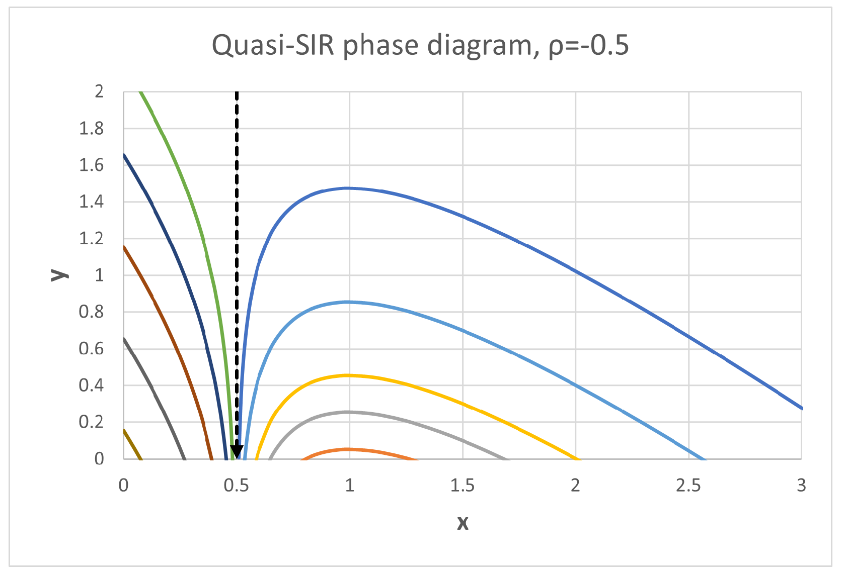
Note that (i.e., , and ) simplifies to the classic SIS model, , and reproduces the classic SIR model Hamiltonian [46]. For we can apply the transformation (23) to end up with the system (24) with , i.e., the classic SIR model in the variables and . In all cases, phase space trajectories are lines of constant “energy”, Hence, they look like in the classic SIR model, extended to negative values, . So, we have a continuum of disease free equilibria, which are neutrally stable for and unstable for . Also, at we have an infinite energy barrier, which cannot be reached from either side, see Figure A1. In fact, for initial condition the explicit solution is given by the vertical line .
Figure A1.
Phase diagram of the quasi-SIR model. increases for and decreases for . The vertical line corresponds to initial condition .
Figure A1.
Phase diagram of the quasi-SIR model. increases for and decreases for . The vertical line corresponds to initial condition .

For initial conditions and we have and , for all , and , where solves . In this case, no epidemic arises and . This is due to the fact that in this region the recovery flow exceeds the sum of infection + vaccination flow .
If , solutions qualitatively behave like in the classical SIR model, i.e., monotonically decreases with for , for and at . Again, we have , where , but this time . Note that necessarily requires , i.e., no epidemic can arise for , as in the classic SIR model. Also, the inverse function can be given explicitly, similarly as in [32].
Lemma A1.
Solutions of the dynamical system (A5) with initial conditions , and “energy” satisfy
Proof.
This follows immediately from . □
Finally, the final size formula for as a function of in Theorem 3 is also obtained by “energy” conservation.
Proof of Theorem 3.
Part (i) follows from the fact that in variables the system becomes a classic SIR model, where the initial conditions and translate to and . Hence and . To prove part (ii), use
Equation (27) follows from and . To prove part (iii), use
Hence, we obtain
where the first term gives the fraction of vaccinated people. Part iii) follows from . □
Appendix C. The SIS Model with Vaccination
The transformation (23) from the SI(R)S model to Hethcote’s model becomes ill-defined for . Epidemiologically, the model with parameters is uninteresting and near trivial. It implies , whence also ; see Remark 3. This is a pure SIS model furnished with a constant vaccination rate from S to R and permanent immunity in R. So, eventually, all people are vaccinated and this model only shows the trivial equilibrium . Global stability in follows from absence of periodic solutions (use as a Dulac function as in [3,4]) and the fact that is forward invariant.
References
- Kermack, W.O.; McKendrick, A.G. A Contribution to the mathematical theory of epidemics. Proc. Roy. Soc. Lond. A 1927, 115, 700–721. [Google Scholar]
- Hethcote, H. Asymptotic behavior and stability in epidemic models. In Proceedings of the Mathematical Problems in Biology, Victoria, BC, Canada, 7–10 May 1973; Lecture Notes in Biomathematics. van den Driessche, P., Ed.; Springer: Berlin/Heidelberg, Germany, 1974; Volume 2, pp. 83–92. [Google Scholar] [CrossRef]
- Hethcote, H. Qualitative analysis for communicable disease models. Math. Biosci. 1976, 28, 335–356. [Google Scholar] [CrossRef]
- Hethcote, H. Three basic epidemiological models. In Applied Mathematical Ecology; Levin, S., Hallam, T., Gross, L., Eds.; Biomathematics Texts; Springer: Berlin/Heidelberg, Germany, 1989; Volume 18, pp. 119–144. [Google Scholar]
- Hethcote, H. The Mathematics of Infectious Diseases. SIAM Rev. 2000, 42, 599. [Google Scholar] [CrossRef] [Green Version]
- Martcheva, M. An Introduction to Mathematical Epidemiology; Number 61 in Texts in Applied Mathematics; Springer: Berlin/Heidelberg, Germany, 2015. [Google Scholar]
- Nill, F. Endemic oscillations for SARS-COV-2 Omicron—A SIRS model analysis. Chaos Solitons Fractals 2023, 173, 113678. [Google Scholar] [CrossRef] [PubMed]
- Nill, F. On the redundancy of birth and death rates in homogenous epidemic SIR models. Fractal Fract. 2023, 7, 313. [Google Scholar] [CrossRef]
- Avram, F.; Adenane, R.; Bianchin, G.; Halanay, A. Stability analysis of an eight parameter SIR- type model including loss of immunity, and disease and vaccination fatalities. Mathematics 2022, 10, 402. [Google Scholar] [CrossRef]
- Kribs-Zaleta, C.; Velasco-Hernandez, J. A simple vaccination model with multiple endemic states. Math. Biosci. 2000, 164, 183–201. [Google Scholar] [CrossRef] [Green Version]
- Li, J.; Ma, Z. Qualitative analyses of SIS epidemic model with vaccination and varying total population size. Math. Comput. Model. 2002, 35, 1235–1243. [Google Scholar] [CrossRef]
- Kopfová, J.; Nábelková, P.; Rachinskii, D.; Rouf, S. Dynamics of SIR model with vaccination and heterogeneous behavioral response of individuals modeled by the Preisach operator. J. Mat. Biol. 2021, 83, 11. [Google Scholar] [CrossRef]
- d’Onofrio, A.; Manfredi, P.; Salinelli, E. Vaccinating behaviour, information, and the dynamics of SIR vaccine preventable diseases. Theor. Popul. Biol. 2007, 71, 301–317. [Google Scholar] [CrossRef]
- d’Onofrio, A.; Manfredi, P.; Salinelli, E. Fatal SIR diseases and rational exemption to vaccination. Math. Med. Bio. 2008, 25, 337–357. [Google Scholar] [CrossRef]
- Korobeinikov, A.; Wake, G. Lyapunov Functions and Global Stability for SIR, SIRS, and SIS Epidemiological Models. Appl. Math. Lett. 2002, 15, 955–960. [Google Scholar] [CrossRef] [Green Version]
- O’Regan, S.; Kelly, T.; Korobeinikov, A.; O’Callaghan, M.; Pokrovskii, A. Lyapunov functions for SIR and SIRS epidemic models. Appl. Math. Lett. 2010, 23, 446–448. [Google Scholar] [CrossRef] [Green Version]
- Ullah, R.; Zaman, G.; Islam, S. Stability analysis of a general SIR epidemic model. VFAST Trans. Math. 2009, 1, 16–20. [Google Scholar]
- Chauhan, S.; Misra, O.; Dhar, J. Stability Analysis of Sir Model with Vaccination. Am. J. Comp. Appl. Math. 2014, 2014, 17–23. [Google Scholar]
- Batistela, C.; Ramos, M.; Cabrera, M.; Dieguez, G.; Piqueira, J. Vaccination and social distance to prevent Covid-19. IFAC-PapersOnLine 2021, 54, 151–156. [Google Scholar] [CrossRef]
- Arino, J.; Mccluskey, C.; van den Driessche, P. Global results for an epidemic model with vaccination that exhibits backwad bifurcation. SIAM J. Appl. Math. 2003, 64, 260–276. [Google Scholar] [CrossRef] [Green Version]
- Alexander, M.; Moghadas, S.; Rohani, P.; Summers, A. Modelling the effect of a booster vaccination on disease epidemiology. J. Math. Biol. 2006, 52, 290–306. [Google Scholar] [CrossRef]
- Lu, Z.; Chi, X.; Chen, L. The effect of constant and pulse vaccination on SIR epidemic model with horizontal and vertical transmission. Math. Comput. Model. 2002, 36, 1039–1057. [Google Scholar] [CrossRef]
- Gao, S.; Teng, Z.; Nieto, J.; Torres, A. Analysis of an SIR Epidemic Model with Pulse Vaccination and Distributed Time Delay. J. Biomed. Biotechnol. 2007, 2007, 64870. [Google Scholar] [CrossRef] [Green Version]
- Shi, P.; Dong, L. Dynamical Models for Infectious Diseases with Varying Population Size and Vaccinations. J. Appl. Math. 2012, 2012, 824192. [Google Scholar] [CrossRef] [Green Version]
- Ledzewicz, U.; Schattler, H. On optimal singular controls for a general SIR- model with vaccination and treatment. Disc. Cont. Dyn. Sys. 2011, 2011, 981–990. [Google Scholar]
- Hadeler, K.P.; Castillo-Chavez, C. A Core Group Model for Disease Transmission. Math.Biosci. 1995, 128, 41–55. [Google Scholar] [CrossRef] [PubMed] [Green Version]
- Hadeler, K.P.; van den Driessche, P. Backward Bifurcation in epidemic Control. Math. Biosci. 1997, 146, 15–35. [Google Scholar] [CrossRef]
- Avram, F.; Adenane, R.; Basnarkov, L.; Bianchin, G.; Goreac, D.; Halanay, A. On matrix-SIR Arino models with linear birth rate, loss of immunity, disease and vaccination fatalities, and their approximations. arXiv 2022, arXiv:2112.03436. [Google Scholar]
- Nill, F. Symmetries and normalization in 3-compartment epidemic models. I: The replacement number dynamics. arXiv 2023, arXiv:2301.00159. [Google Scholar] [CrossRef]
- van den Driessche, P. Reproduction numbers of infectious disease models. Infect. Dis. Model. 2017, 2, 288–303. [Google Scholar] [CrossRef]
- Hethcote, H. Note on determining the limiting susceptible population in an epidemic model. Math. Biosci. 1970, 9, 161–163. [Google Scholar] [CrossRef]
- Harko, T.; Lobo, F.; Mak, M. Exact analytical solutions of the susceptible-infected-recovered (SIR) epidemic model and of the SIR model with equal death and birth rates. Appl. Math. Comput. 2014, 236, 184–194. [Google Scholar] [CrossRef] [Green Version]
- Prodanov, D. Comments on some analytical and numerical aspects of the SIR model. Appl. Math. Model. 2021, 95, 236–243. [Google Scholar] [CrossRef]
- The Lambert W-Function. Available online: https://mathworld.wolfram.com/LambertW-Function.html (accessed on 19 June 2023).
- Corless, R.; Gonnet, G.; Hare, D.; Jeffrey, D.; Knuth, D. On the Lambert W function. Adv. Comput. Math. 1996, 5, 329–359. [Google Scholar] [CrossRef]
- Ma, J.; Earn, D.J. Generality of the final size formula for an epidemic of a newly invading infectious disease. Bull. Math. Biol. 2006, 68, 679–702. [Google Scholar] [CrossRef] [PubMed]
- Miller, J.C. A Note on the Derivation of Epidemic Final Sizes. Bull. Math. Biol. 2012, 74, 2125–2141. [Google Scholar] [CrossRef]
- Weiss, H.H. The SIR model and the Foundations of Public Health. Mater. Math. 2013, 2013, 17. [Google Scholar]
- Brenig, L. Reducing nonlinear dynamical systems to canonical forms. Phil. Trans. R. Soc. A 2018, 376, 20170384. [Google Scholar] [CrossRef] [Green Version]
- Hernández-Bermejo, B.; Fairén, V. Hamiltonian structure and Darboux theorem for families of generalized Lotka–Volterra systems. J. Math. Phys. 1998, 39, 6162–6174. [Google Scholar] [CrossRef] [Green Version]
- Busenberg, S.N.; van den Driessche, P. Analysis of a disease transmission model in a population with varying size. J. Math. Biol. 1990, 28, 257–270. [Google Scholar] [CrossRef] [PubMed] [Green Version]
- Mena-Lorca, J.; Hethcote, H. Dynamic models of infectious diseases as regulators of population sizes. J. Math. Biol 1992, 30, 693–716. [Google Scholar] [CrossRef] [PubMed]
- Derrick, W.; van den Driessche, P. A disease transmission model in a nonconstant population. J. Math. Biol. 1993, 31, 495–512. [Google Scholar] [CrossRef]
- Vargas-De-León, C. On the global stability of SIS, SIR and SIRS epidemic models with standard incidence. Chaos Solitons Fractals 2011, 44, 1106–1110. [Google Scholar] [CrossRef]
- d’Onofrio, A.; Manfredi, P.; Salinelli, E. Lyapunov stability of an SIRS epidemic model with varying population. arXiv 2018, arXiv:1812.10676. [Google Scholar] [CrossRef]
- Gümral, H.; Nutku, Y. Poisson Structure of dynamical systems with three degrees of freedom. J. Math. Phys. 1993, 34, 5691–5723. [Google Scholar] [CrossRef] [Green Version]
Figure 1.
Flow diagram of the SIR model.

Figure 2.
Standard models featuring endemic equilibria.

Figure 3.
Flow diagram of the SI(R)S model. denotes the number of not infected newborns per unit of time.
Figure 3.
Flow diagram of the SI(R)S model. denotes the number of not infected newborns per unit of time.

Disclaimer/Publisher’s Note: The statements, opinions and data contained in all publications are solely those of the individual author(s) and contributor(s) and not of MDPI and/or the editor(s). MDPI and/or the editor(s) disclaim responsibility for any injury to people or property resulting from any ideas, methods, instructions or products referred to in the content. |
© 2023 by the author. Licensee MDPI, Basel, Switzerland. This article is an open access article distributed under the terms and conditions of the Creative Commons Attribution (CC BY) license (https://creativecommons.org/licenses/by/4.0/).
Share and Cite
MDPI and ACS Style
Nill, F. Scaling Symmetries and Parameter Reduction in Epidemic SI(R)S Models. Symmetry 2023, 15, 1390. https://doi.org/10.3390/sym15071390
AMA Style
Nill F. Scaling Symmetries and Parameter Reduction in Epidemic SI(R)S Models. Symmetry. 2023; 15(7):1390. https://doi.org/10.3390/sym15071390
Chicago/Turabian StyleNill, Florian. 2023. "Scaling Symmetries and Parameter Reduction in Epidemic SI(R)S Models" Symmetry 15, no. 7: 1390. https://doi.org/10.3390/sym15071390
Note that from the first issue of 2016, this journal uses article numbers instead of page numbers. See further details here.