Visco-Elastic Interface Effect on the Dynamic Stress of Symmetrical Tunnel Embedded in a Half-Plane Subjected to P Waves

Abstract

A semi-analytical method is developed to study the visco-elastic interface effect on the dynamic stress of a non-circular symmetrical tunnel in a half-plane subjected to P waves, and the interaction between the visco-elastic interface around the tunnel and the traction free boundary at the half-plane is analyzed. The complex variable function method combined with the wave function expansion method is introduced to obtain the theoretical expressions of waves around the non-circular tunnel. To satisfy the traction-free boundary condition at the half-plane, the large circle assumption is applied. The expanded coefficients are determined by using appropriate boundary conditions with stiffness parameters and viscosity coefficients of the interface. Selected numerical results are presented, and the interface effect on the dynamic stress under different embedded depths is discussed. It is found that the interacting effect of the visco-elastic interface and the traction-free boundary is quite related with the wave frequency. Comparison with existing results is also given to validate the semi-analytical method.

1. Introduction

The effect of local inhomogeneities on seismic wave propagation is a fundamental subject in several engineering disciplines, such as civil engineering, earthquake engineering, and mechanical engineering [1,2,3]. The dynamic stress concentration around the local inclusions due to seismic waves has attracted lots of attention in the past decade. The analytical method (the wave function expansion method) and numerical methods (the finite differences, the finite elements, the boundary integral equations, or the discrete wave number method) have been extensively applied to solve the dynamic problem.

Since the pioneering work of Pao and Mao [4], the wave function expansion method has been widely used in solving the diffraction of P, SV, and SH waves around the regular inclusions such as arbitrary-shape inclusions [5], elliptic cavities [6], two cylindrical cavities [7], and so on. In past decades, the diffraction of elastic waves around the tunnels was also studied. Moore and Guan studied the dynamic stress around the lined tunnel subjected to seismic loading in an infinite medium using the successive reflection method [8]. The seismic response of a linear and elastic medium embedded with an unlined tunnel subjected to vertically propagating SV and P waves was addressed [9]. Wang et al. applied the dynamic finite element method to analyze the effect of layered rocks on the dynamic response of a tunnel subjected to P and S waves [10]. By using the complex variable method, the dynamic stress concentration of twin closely spaced circular tunnels under plane P and SV waves in a full space was derived [11]. For the circular cylindrical cavity [12], elliptic cavities [13], spherical cavities [14], and tunnels [15] in the fluid-saturated porous medium, the dynamic stress resulting from the elastic waves has been addressed in the past decades.

The interface between the tunnel and the surrounding medium plays an important role in controlling the dynamic strength of tunnels. The above-mentioned numerical and analytical solutions focused on the perfect interfaces around the tunnels. To optimize the strength of the interface, different interface models were proposed. By using the numerical finite element method, Hassan et al. described the soil–tunnel interaction with contact conditions, and the potentially unrealistic normal tensile and tangential forces at the interface were predicted [16]. An elastic interface was assumed between the tunnel and the surrounding medium, and the dynamic stress concentration factors around the tunnel were evaluated [3].

To construct a practical model, the boundary condition at the half-plane is also an important factor. In the past, an infinite plane was often assumed, and the simplified model cannot describe the effect of the boundary at the half-plane. To optimize the design of tunnels under dynamic loadings, a visco-elastic interface model in a half-plane is proposed in this paper.

The aim of this paper is to present the analytical solutions of displacements and stresses resulting from the visco-elastic interface around the non-circular symmetrical tunnels embedded in a half-plane. The interaction between the interface and the traction-free boundary is considered. To analyze the effect of embedded depth, the surface at the half-plane is approximated as a convex circular surface. Combining the wave function expansion method and conformal transformation method, the analytical expressions are found for displacements and stresses in the tunnel lining and surrounding medium, and the expanded coefficients are determined by satisfying the boundary conditions with the stiffness parameters and viscosity coefficients of the interface. In numerical examples, the effects of stiffness parameters and viscosity coefficients of interface on the dynamic stress under different embedded depths are examined in detail.

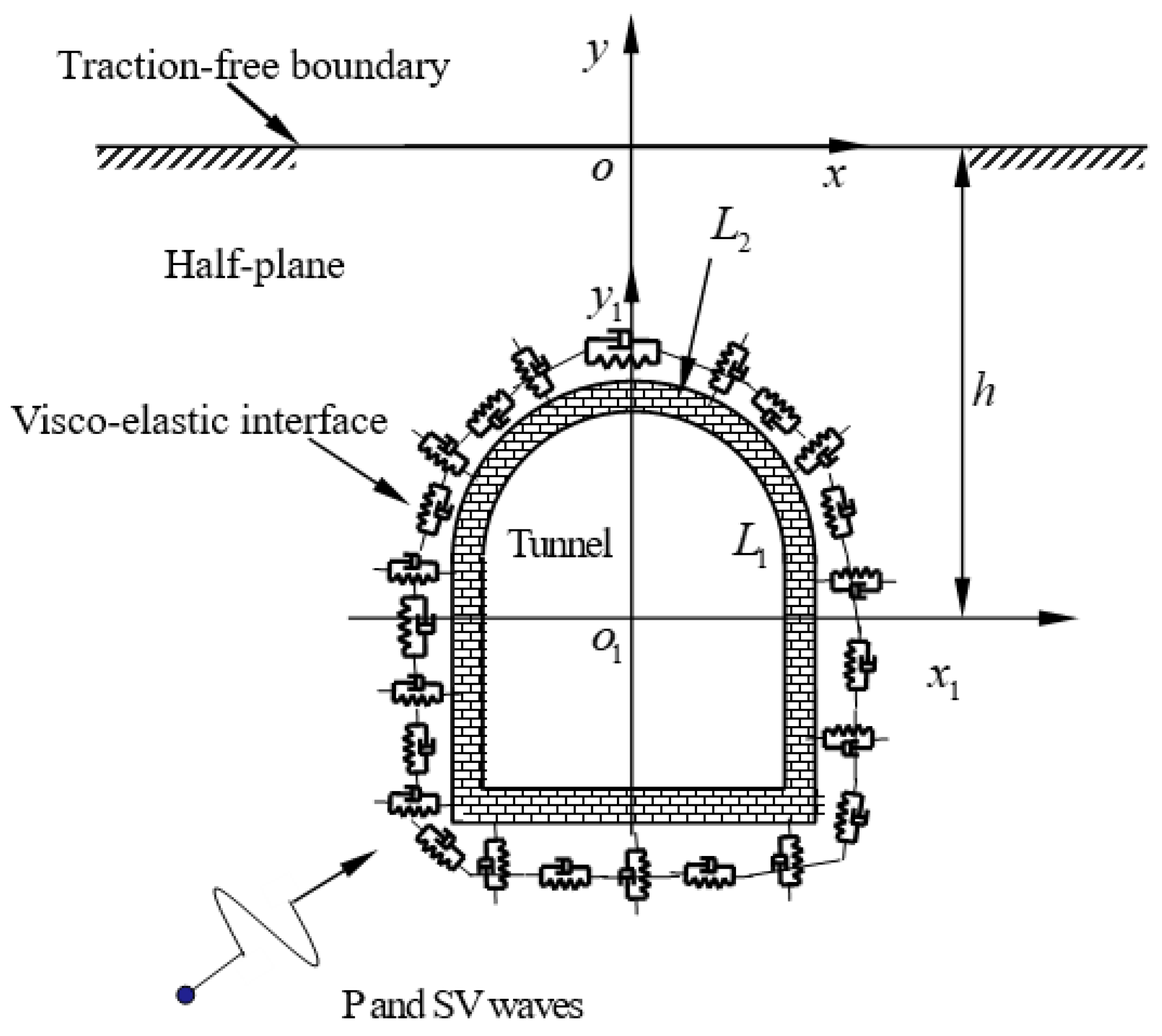
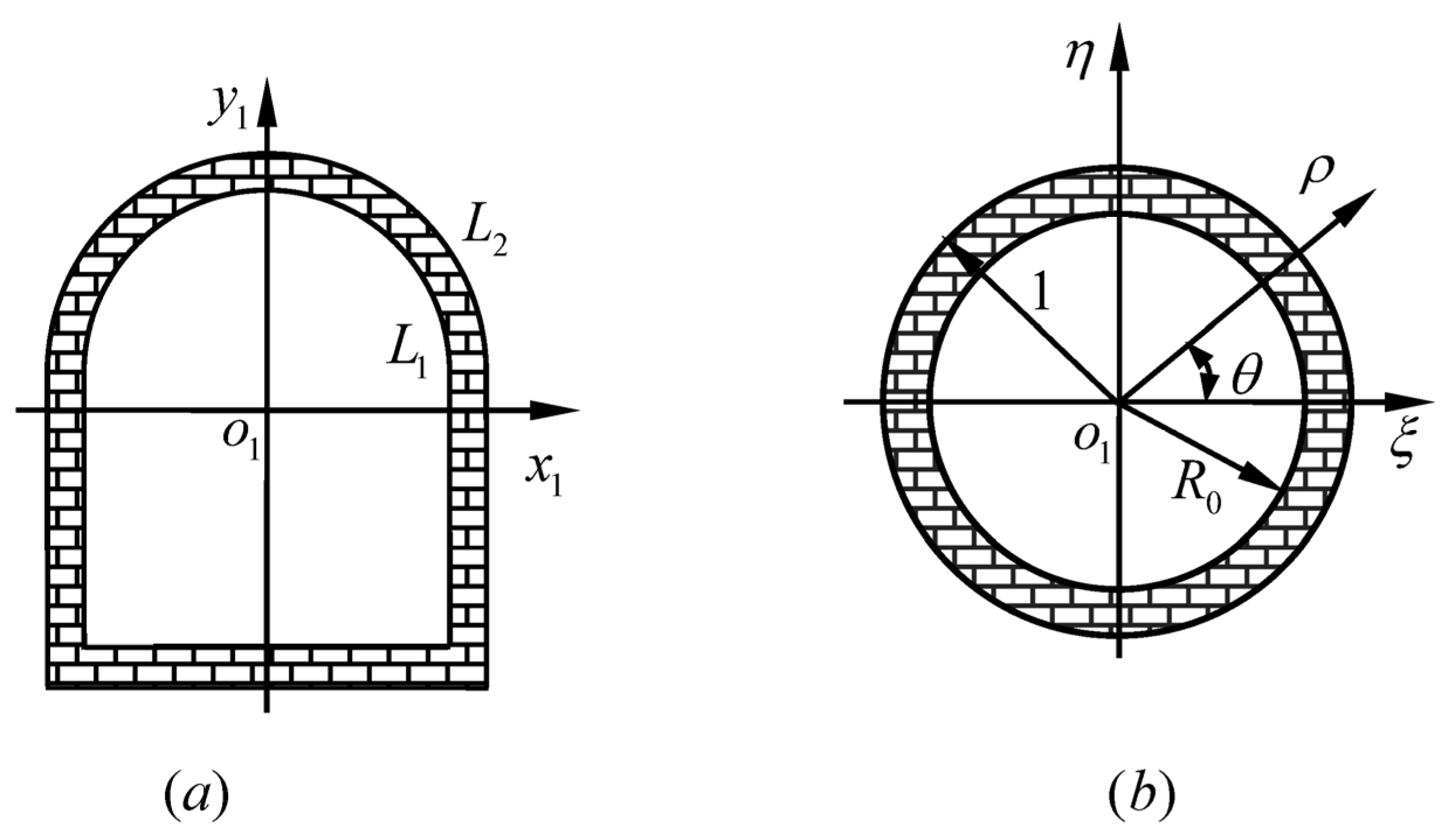
2. Problem Formulation and Basis Solutions

A lined non-circular symmetrical tunnel in a half-plane subjected to P and SV waves is considered, as depicted in Figure 1. The embedded depth of tunnel is h. A visco-elastic interface exists around the tunnel. The traction-free boundary at the surface of the half-plane is assumed. For convenience, it is assumed that the tunnel and the half-plane are both linear isotropic and elastic. The tunnel is bounded by contours L₁ and L₂, and the traction-free boundary is denoted by F. The Lame constants and density of the half-plane are denoted by ${\lambda }_H$, ${\mu }_H$, and ${\rho }_H$, and those of tunnel lining are ${\lambda }_L$, ${\mu }_L$, and ${\rho }_L$. Due to the geometrical characteristics and the characteristics of applied loading, this problem can be simplified into a plane strain problem. The harmonic P waves generated by the harmonic dilatational line source located at $\overline{o}$ propagate in the half-plane.

To obtain the analytical solution of a non-circular symmetrical tunnel, the conformal mapping method of a complex function is employed, i.e.,

$$z=g(\zeta )=\overline{R}\left(\zeta +{\displaystyle \sum _{m=0}^n{c}_m{\zeta }^{-m}}\right) \zeta =\xi +\mathrm{i}\eta =\rho e^{\mathrm{i}\theta }.$$

(1)

where $\overline{R}$ and $c_m$ can be solved by the method described in [17]. The mapping function transforms the non-circular symmetrical tunnel in the z plane ($o_1{x}_1{y}_1$) into the annular region in the $\zeta$ plane, as shown in Figure 2. The outer radius and inner radius are $\left|\zeta \right|=1$ and $\left|\zeta \right|=R_0$, respectively. Because the tunnel is symmetrical about the y₁ axis, the coefficients $c_m$ must be real numbers. All coefficients in the mapping function can be determined when the shape of the cross-section of the tunnel and the support thickness are known.

3. Wave Fields in the Rock Mass and Concrete Lining

The governing equation for the linear and elastic medium can be expressed as

$$\mu u_{i,jj}+(\lambda +\mu )u_{j,ji}=\rho {\ddot{u}}_i i,j=x,y$$

(2)

where $u$ is the displacement in the medium.

Following the Helmholtz decomposition method, the scalar potential $\phi$ and vector potential $\psi$ are introduced to express the displacements and stresses in the tunnel and surrounding medium. The Helmholtz equations of these potentials are expressed as

$${\nabla }^2\phi +k_p^2\phi =0$$

(3)

$${\nabla }^2\psi +k_s^2\psi =0$$

(4)

where $k_p=\omega /V_p$ is the wave number of the compressional waves, $V_p=\sqrt{(\lambda +2\mu )/\rho }$, $k_s=\omega /V_s$ is the wave number of the shear waves, and $V_s=\sqrt{\mu /\rho }$.

3.1. The Incident Waves

An infinitely long lined tunnel with a visco-elastic interface in a half-plane is considered. In the steady-state case, a harmonic incident wave generated by the harmonic dilatational line source can be expressed, in the z plane, as [4]

$${\phi }_1^{(in)}={\phi }_0{\displaystyle \sum _{n=0}^{\infty }{(-1)}^n{\epsilon }_n{H}_n^{(1)}(k_{p1}{r}_0)J_n(k_{p1}|z|)\cos n{\theta }_1{e}^{-\mathrm{i}\omega t}}$$

(5)

where ${\phi }_0$ is the amplitude of incident P waves, ${\epsilon }_n=1$ for $n=0$, ${\epsilon }_n=2$ for $n\ge 1$, $k_{p1}$ is the wave number in the half-plane, $r_0$ is the distance between the center of the tunnel and the line source, $H_n^{(1)}(·)$ is the nth Hankel function of the first kind, and $J_n(·)$ is the nth Bessel function. The subscript 1 denotes the rock mass. The superscript (in) denotes the incident waves.

3.2. The Scattered Field in the Half-Plane

When the incident P wave runs into the lined tunnel, two waves at the interface come into being. The displacement potentials of scattered waves are written, in the z plane, as [4]

$${\phi }_1^{(sc)}={\displaystyle \sum _{n=0}^{\infty }{A}_n}{H}_n^{(1)}(k_{p1}|z|)\cos n{\theta }_1{e}^{-\mathrm{i}\omega t}$$

(6)

$${\psi }_1^{(sc)}={\displaystyle \sum _{n=0}^{\infty }{B}_n}{H}_n^{(1)}(k_{s1}|z|)\sin n{\theta }_1{e}^{-\mathrm{i}\omega t}$$

(7)

where $A_n$ and $B_n$ are the expanded coefficients and $k_{s1}$ is the wave number of the SV waves in the half-plane. The superscript (sc) denotes the scattered waves.

3.3. The Reflected Field in the Tunnel Lining

There are two reflected waves propagating outwards from the inner boundary of concrete tunnel. They are confined inside the tunnel lining, and can be represented by [4]

$${\phi }_2^{(rl)}={\displaystyle \sum _{n=0}^{\infty }{C}_n}{H}_n^{(1)}(k_{p2}|z|)\cos n{\theta }_1{e}^{-\mathrm{i}\omega t}$$

(8)

$${\psi }_2^{(rl)}={\displaystyle \sum _{n=0}^{\infty }{E}_n}{H}_n^{(1)}(k_{s2}|z|)\sin n{\theta }_1{e}^{-\mathrm{i}\omega t}$$

(9)

where $C_n$ and $E_n$ are the mode coefficients of reflected waves around the lining, $k_{p2}$ is the wave number of the P waves in the tunnel lining, and $k_{s2}$ is the wave number of the SV waves in the tunnel lining. The subscript 2 denotes the tunnel lining. The superscript (rl) denotes the reflected waves.

3.4. The Refracted Field Inside the Tunnel Lining

Inside the lined tunnel, there are two refracted waves that propagate inside the lining from the outer boundary of the tunnel. The displacement fields of the refracted waves are given by [4]

$${\phi }_2^{(rr)}={\displaystyle \sum _{n=0}^{\infty }{D}_n}{H}_n^{(2)}(k_{p2}|z|)\cos n{\theta }_1{e}^{-\mathrm{i}\omega t}$$

(10)

$${\psi }_2^{(rr)}={\displaystyle \sum _{n=0}^{\infty }{F}_n}{H}_n^{(2)}{k}_{s2}\left|z\right|)\sin n{\theta }_1{e}^{-\mathrm{i}\omega t}$$

(11)

where $D_n$ and $F_n$ are the mode coefficients of refracted waves in the tunnel lining and $H_n^{(2)}(·)$ is the nth Hankel function of the second kind.

3.5. The Wave Fields from the Half-Plane

Because of the straight border of the half-plane, two reflected waves resulting from the incident P waves occur in the half-plane. They are expressed as [18]

$${\phi }_3^{(rl)}=\overline{\phi }{e}^{\frac{\mathrm{i}{k}_{p1}}{2}\left[\zeta e^{\mathrm{i}\alpha }+\overline{\zeta }{e}^{-\mathrm{i}\alpha }\right]}$$

(12)

$${\psi }_3^{(rl)}=\tilde{\phi }{e}^{\frac{\mathrm{i}{k}_{s1}}{2}\left[\zeta e^{\mathrm{i}\beta }+\overline{\zeta }{e}^{-\mathrm{i}\beta }\right]}$$

(13)

where the subscript 3 denotes the straight border, $\overline{\phi }$ and $\tilde{\phi }$ are the amplitudes of the reflected waves, and $\alpha$ and $\beta$ are the reflection angles. They can be written as [18]

$$\overline{\phi }={\phi }_0\frac{\sin 2\beta \sin 2{\alpha }_0-{(k_{s1}/k_{p1})}^2{\cos }^{2}2\beta }{{(k_{s1}/k_{p1})}^2{\cos }^{2}2\beta +\sin 2\beta \sin 2{\alpha }_0}$$

(14)

$$\tilde{\phi }=\frac{2{\phi }_0\sin 2{\alpha }_0\cos 2\beta }{{(k_{s1}/k_{p1})}^2{\cos }^{2}2\beta +\sin 2\beta \sin 2{\alpha }_0}$$

(15)

$$\alpha ={\alpha }_0$$

(16)

$$\beta ={\cos }^{-1}(\frac{k_{p1}}{k_{s1}}\cos {\alpha }_0)$$

(17)

where ${\alpha }_0$ is incident angle of the P waves. For convenience, it is assumed that ${\alpha }_0=\pi /2$.

To satisfy the traction-free boundary condition, the half-plane surface is approximated as a convex circular surface centered at o₂ with large radius $R\gg R_0$, as shown in Figure 3. It is now obvious that when the radius of the large circle approaches infinity, this model approaches that of the non-circular tunnel in the half-plane. Such an approximation may result in a calculation error when the tunnel has a shallow overburden. For instance, the depth of a tunnel is $h=2R_0$. By selecting a large radius R, the error can be reduced.

At the surface of the half-plane, the scattering waves from the non-circular tunnel will be reflected, and the reflected P and SV waves are expressed as [4]

$${\overline{\phi }}^{(rl)}={\displaystyle \sum _{n=0}^{\infty }{M}_n}{H}_n^{(1)}(k_{p1}R)\cos n{\theta }_2{e}^{-\mathrm{i}\omega t}$$

(18)

$${\overline{\psi }}^{(rl)}={\displaystyle \sum _{n=0}^{\infty }{N}_n}{H}_n^{(1)}(k_{s1}R)\sin n{\theta }_2{e}^{-\mathrm{i}\omega t}$$

(19)

where $M_n$ and $N_n$ are the expanded coefficients of waves in the rock mass and $R$ is the radius of the large circular arc.

3.6. The Total Displacement Potential in the Half-Plane and Concrete Tunnel

The total displacement potential in the half-plane is produced by the superposition of the incident waves, the reflected waves at the surface of the half-plane, and the scattered waves resulting from the tunnel, i.e.,

$$\begin{array}{l}{\phi }_1^{(t)}={\displaystyle \sum _{n=0}^{\infty }\left[{\phi }_0{(-1)}^n{\delta }_n{H}_n^{(1)}(k_{p1}{r}_0)J_n(k_{p1}|z|)+A_n{H}_n^{(1)}(k_{p1}|z|)\right]\cos n{\theta }_1{e}^{-\mathrm{i}\omega t}}\\ +{\displaystyle \sum _{n=0}^{\infty }{M}_n}{H}_n^{(1)}(k_{p1}R)\cos n{\theta }_2{e}^{-\mathrm{i}\omega t}+{\phi }_1{e}^{\frac{\mathrm{i}{k}_{p1}}{2}\left[\zeta e^{\mathrm{i}{\alpha }_1}+\overline{\zeta }{e}^{-\mathrm{i}{\alpha }_1}\right]}\end{array}$$

(20)

$${\psi }_1^{(t)}={\displaystyle \sum _{n=0}^{\infty }{B}_n{H}_n^{(1)}(k_{s1}|z|)}\sin n{\theta }_1{e}^{-\mathrm{i}\omega t}+{\displaystyle \sum _{n=0}^{\infty }{N}_n}{H}_n^{(1)}(k_{s1}R)\sin n{\theta }_2{e}^{-\mathrm{i}\omega t}+{\phi }_2{e}^{\frac{\mathrm{i}{k}_{s1}}{2}\left[\zeta e^{\mathrm{i}{\alpha }_2}+\overline{\zeta }{e}^{-\mathrm{i}{\alpha }_2}\right]}$$

(21)

The total displacement potential in the concrete lining of tunnel is produced by the superposition of the refracted waves and the reflected waves resulting from the inner boundary of the lining, i.e.,

$${\phi }_2^{(t)}={\displaystyle \sum _{n=0}^{\infty }\left[C_n{H}_n^{(1)}(k_{p2}|z|)+D_n{H}_n^{(2)}(k_{p2}|z|)\right]\cos n{\theta }_1{e}^{-\mathrm{i}\omega t}}$$

(22)

$${\psi }_2^{(t)}={\displaystyle \sum _{n=0}^{\infty }\left[E_n{H}_n^{(1)}(k_{s2}|z|)+F_n{H}_n^{(2)}(k_{s2}|z|)\right]}\sin n{\theta }_1{e}^{-\mathrm{i}\omega t}$$

(23)

To make computation tractable, the expressions of displacement potentials in the local coordinate system ($r_2$,${\theta }_2$) should be transformed into another local coordinate system ($r_1$,${\theta }_1$). According to the addition theorem for the Bessel function, the following relation can be derived [19].

$$H_n^{(1)}(\kappa r_2)e^{\mathrm{i}n{\theta }_2}={\displaystyle \sum _{s=-\infty }^{\infty }{e}^{\mathrm{i}(s-n){\theta }_{21}}}{H}_{s-n}^{(1)}(\kappa r_{21})J_s(\kappa r_1)e^{\mathrm{i}s{\theta }_1}$$

(24)

Similarly,

$$H_n^{(1)}(\kappa r_1)e^{\mathrm{i}n{\theta }_1}={\displaystyle \sum _{s=-\infty }^{\infty }{e}^{\mathrm{i}(s-n){\theta }_{12}}}{H}_{s-n}^{(1)}(\kappa r_{12})J_s(\kappa r_2)e^{\mathrm{i}s{\theta }_2}$$

(25)

It is noted that ${\theta }_{12}=\pi /2$, ${\theta }_{21}=3\pi /2$ and $r_{12}=r_{21}=R+h$ are shown in Figure 3.

4. Boundary Conditions and Solving the Expanded Coefficients

To analyze the interacting effect of the visco-elastic interface and the half-plane, the following interface model is introduced. In this model, it is assumed that the tractions at the outer boundary of tunnel lining are continuous and the normal and circumferential displacements are not continuous. The stiffness parameter and viscosity coefficient of the imperfect interface are introduced to characterize the visco-elastic effect.

Using this model, the boundary conditions at the interfaces of the concrete lining (L₂ in Figure 1) can be described as follows:

$${\sigma }_{rr1}={\sigma }_{rr2}$$

(26)

$${\sigma }_{r\theta 1}={\sigma }_{r\theta 2}$$

(27)

$$u_{r1}-u_{r2}+{\delta }_r\frac{\partial (u_{r1}-u_{r2})}{\partial t}=\frac{{\sigma }_{rr1}}{k_r}$$

(28)

$$u_{\theta 1}-u_{\theta 2}+{\delta }_{\theta }\frac{\partial (u_{\theta 1}-u_{\theta 2})}{\partial t}=\frac{{\sigma }_{r\theta 1}}{k_{\theta }}$$

(29)

where $k_r$ and $k_{\theta }$ are the stiffness parameters of the imperfect interface and ${\delta }_r$ and ${\delta }_{\theta }$ are the viscosity coefficients of the imperfect interface.

At the inner boundary of the concrete lining (L₁ in Figure 1), it is assumed that the tractions are free. It can be expressed as:

$${\sigma }_{rr2}=0$$

(30)

$${\sigma }_{r\theta 2}=0$$

(31)

The traction-free boundary conditions at the surface of the half-plane can be expressed as:

$${\sigma }_{rr3}=0$$

(32)

$${\sigma }_{r\theta 3}=0$$

(33)

The stresses used in the boundary conditions can be solved based on the relations between the displacement potentials, stresses, and displacements. The relations are expressed as:

$${\sigma }_{rr}+{\sigma }_{\theta \theta }=-2k_{p1}^2(\lambda +\mu )\phi$$

(34)

$${\sigma }_{rr}-\mathrm{i}{\sigma }_{r\theta }=-4\mu \frac{{\partial }^2}{\partial {\zeta }^2}(\phi +\mathrm{i}\psi )e^{2\mathrm{i}\theta }-(\lambda +\mu )k_{p1}^2\phi$$

(35)

$${\sigma }_{rr}+\mathrm{i}{\sigma }_{r\theta }=-4\mu \frac{{\partial }^2}{\partial {\overline{\zeta }}^2}(\phi -\mathrm{i}\psi )e^{-2\mathrm{i}\theta }-(\lambda +\mu )k_{p1}^2\phi$$

(36)

$$u_r+\mathrm{i}{u}_{\theta }=2\frac{\partial }{\partial \overline{\zeta }}(\phi -\mathrm{i}\psi )e^{-\mathrm{i}\theta }$$

(37)

$$u_r-\mathrm{i}{u}_{\theta }=2\frac{\partial }{\partial \zeta }(\phi +\mathrm{i}\psi )e^{\mathrm{i}\theta }$$

(38)

Substituting Equations (20)–(23) into Equations (30)–(33), a set of linear algebra equations can be obtained as follows:

$$\left[\begin{array}{cccccccc}{X}_{11}& X_{12}& X_{13}& X_{14}& X_{15}& X_{16}& X_{17}& X_{18}\\ X_{21}& X_{22}& X_{23}& X_{24}& X_{25}& X_{26}& X_{27}& X_{28}\\ X_{31}& X_{32}& X_{33}& X_{34}& X_{35}& X_{36}& X_{37}& X_{38}\\ X_{41}& X_{42}& X_{43}& X_{44}& X_{45}& X_{46}& X_{47}& X_{48}\\ 0& 0& X_{53}& X_{54}& X_{55}& X_{56}& 0& 0\\ 0& 0& X_{63}& X_{64}& X_{65}& X_{66}& 0& 0\\ X_{71}& X_{72}& 0& 0& 0& 0& X_{77}& X_{78}\\ X_{81}& X_{82}& 0& 0& 0& 0& X_{87}& X_{88}\end{array}\right]\left[\begin{array}{c}{A}_n\\ B_n\\ C_n\\ D_n\\ E_n\\ F_n\\ M_n\\ N_n\end{array}\right]=\left[\begin{array}{c}{Y}_{11}\\ Y_{21}\\ Y_{31}\\ Y_{41}\\ 0\\ 0\\ Y_{71}\\ Y_{81}\end{array}\right]$$

(39)

The elements in this matrix equation can be found in Appendix A. The coefficients $A_n$, $B_n$, $C_n$, $D_n$, $E_n$, $F_n$, $M_n$, $N_n$ can be determined by solving Equation (39).

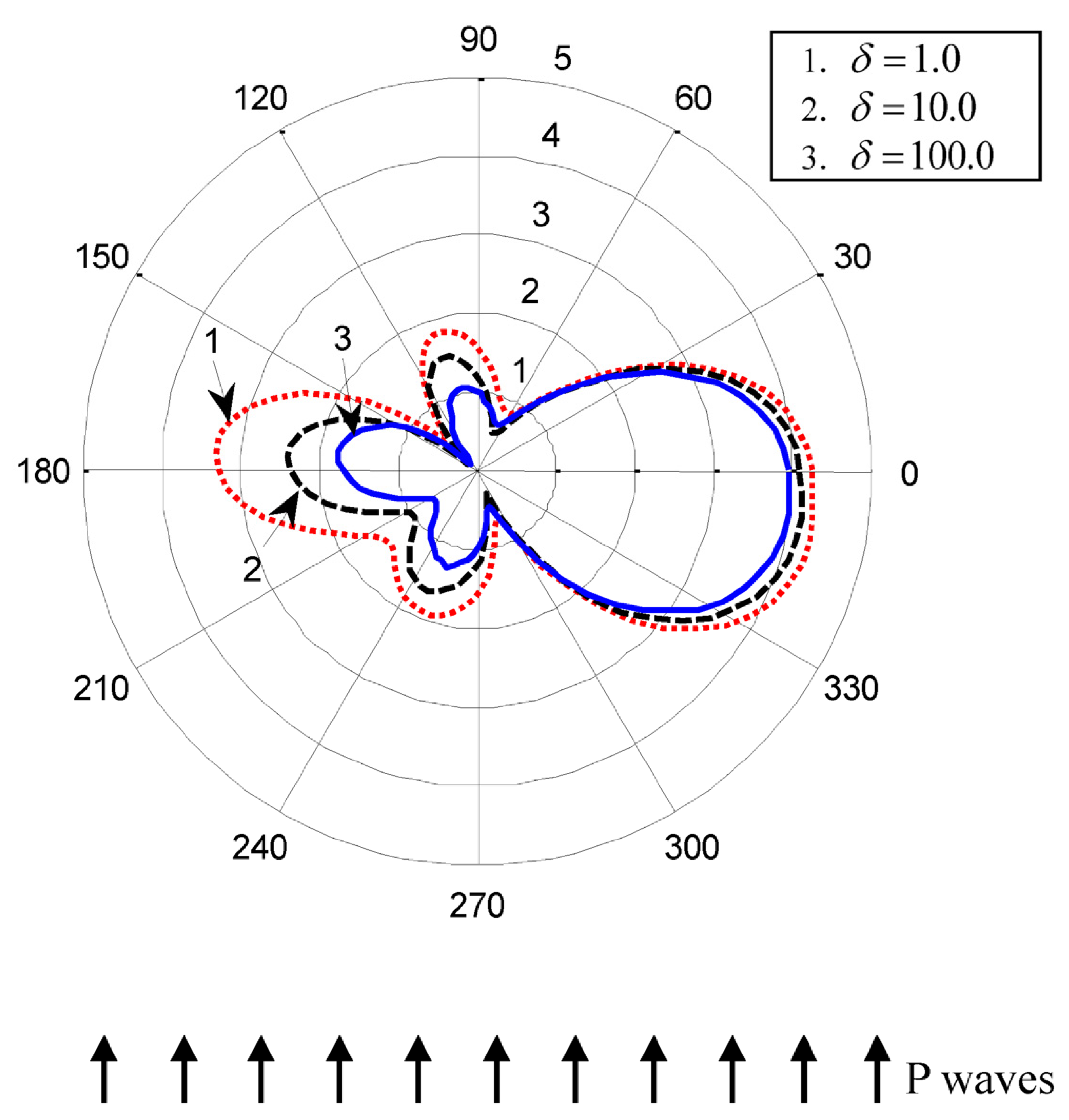
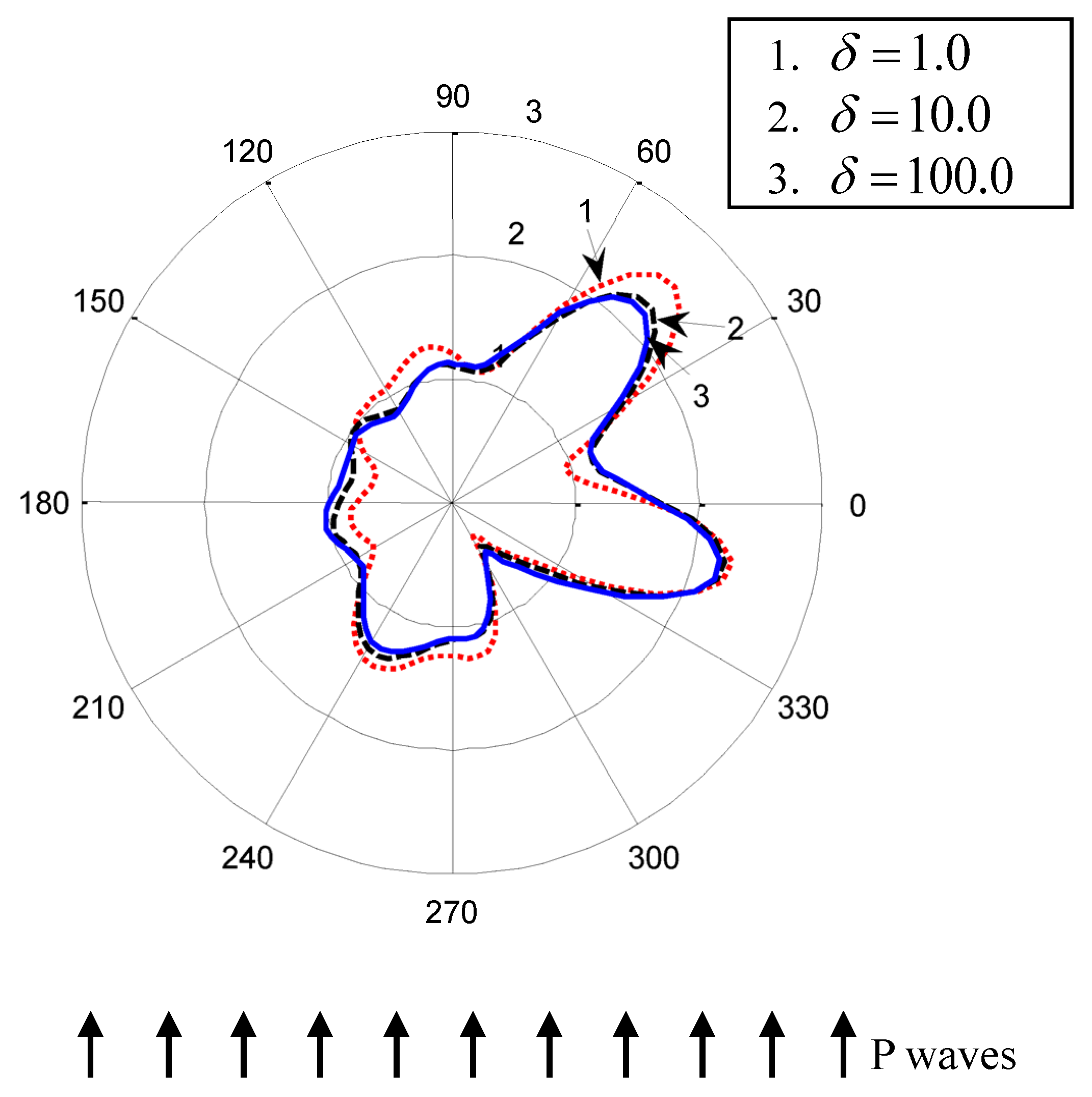
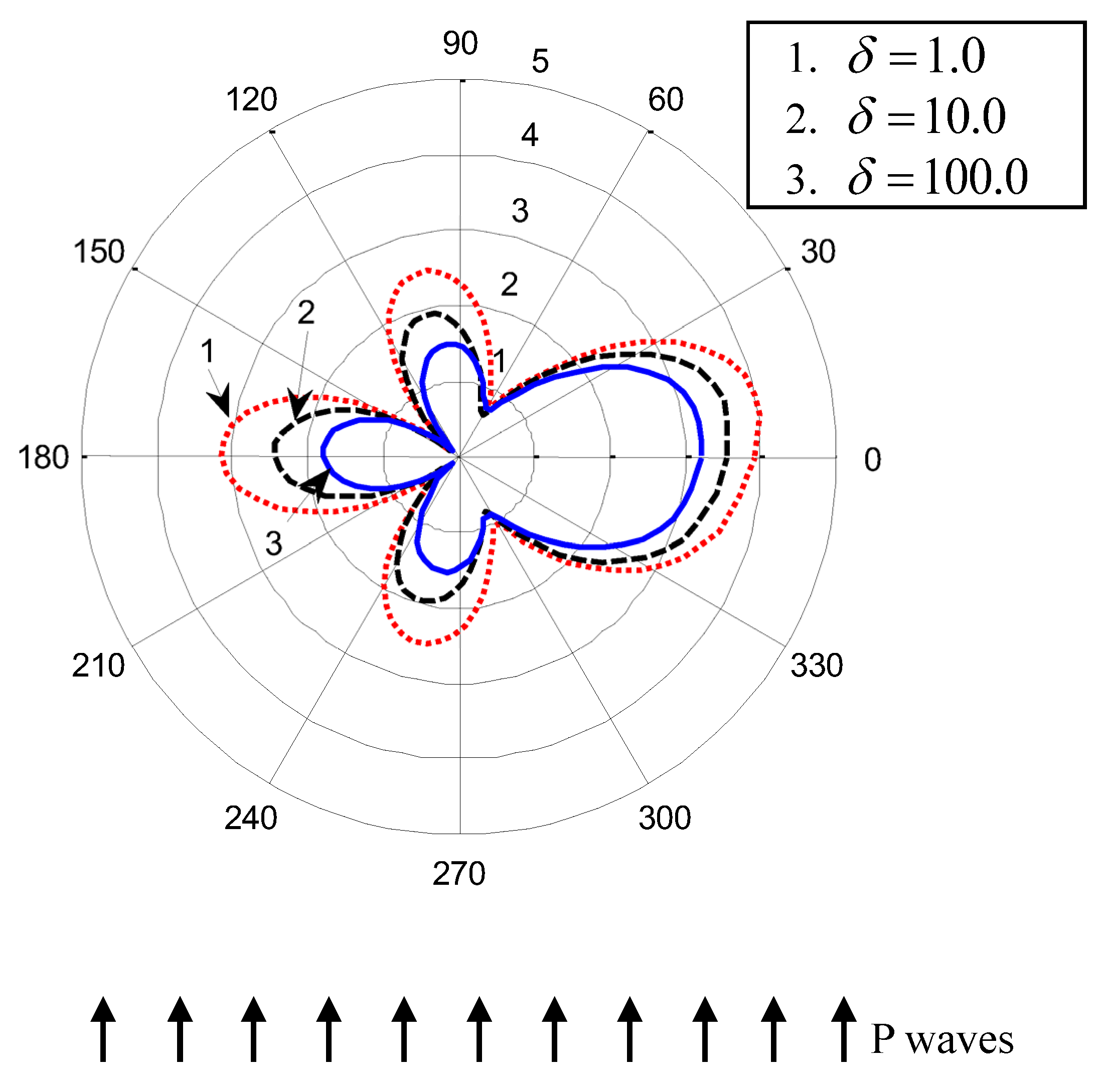
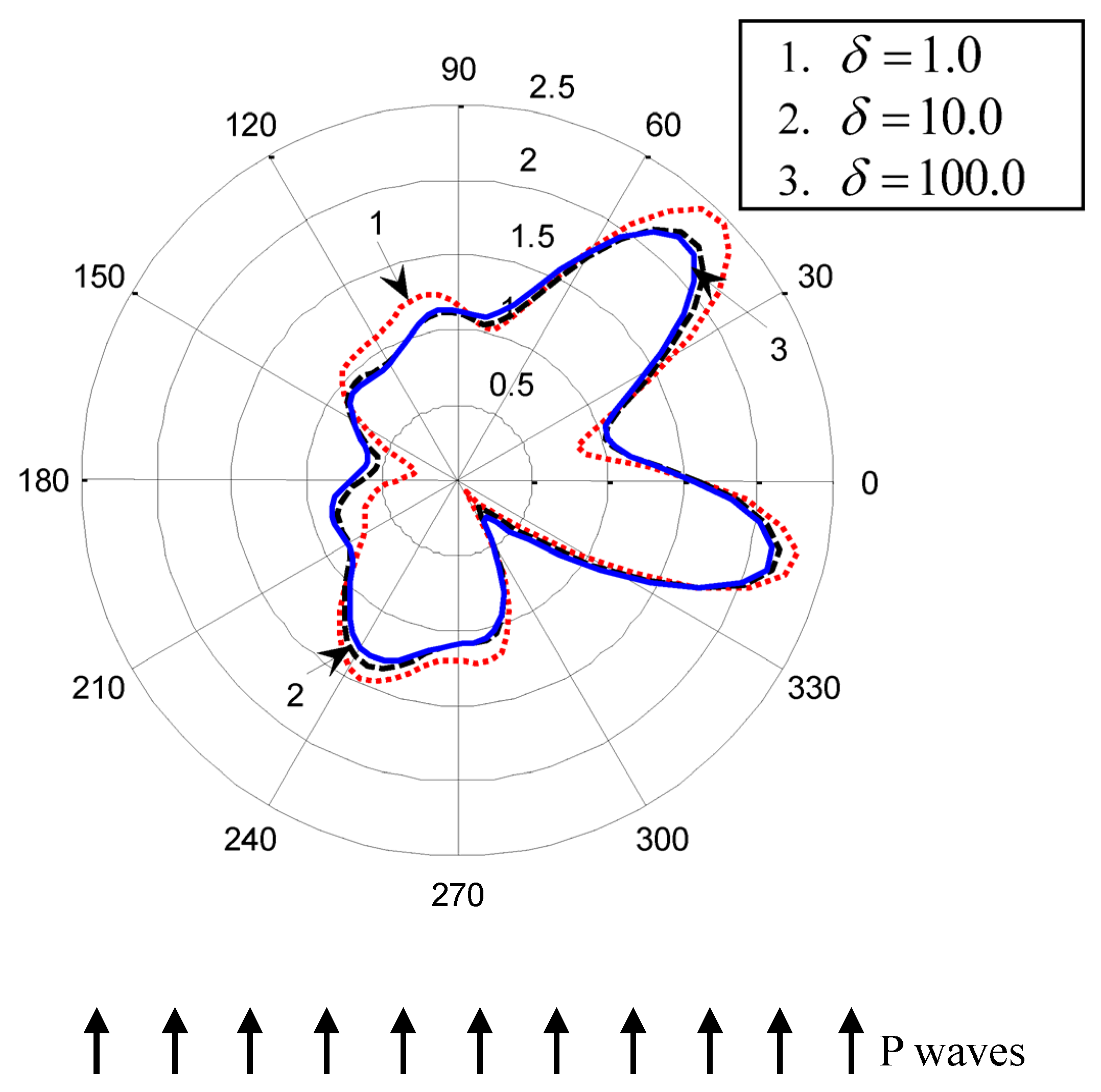
5. Numerical Examples and Analysis

To analyze the visco-elastic boundary effect on the dynamic response of the non-circular tunnel under different loading frequencies, the dimensionless circumferential stress is introduced. According to the definition of the dynamic stress concentration factor (DSCF), the DSCF is the ratio of the circumferential stress ${\sigma }_{\theta \theta }^{}$ around the tunnel and the maximum dynamic stress. Thus, the DSCF around the non-circular tunnel is expressed as [4]

$$DSCF={\sigma }_{\theta \theta }^{\ast }=|{\sigma }_{\theta \theta }/{\sigma }_0|$$

(40)

where ${\sigma }_0$ is the maximum magnitude of stress in the incident direction and ${\sigma }_0={\mu }_H{k}_{p1}^2{\phi }_0$.

To ensure the displacements on the curved surface approach accurately enough to those of a flat surface in the free field, it is assumed that $R=100R_0$. The main objective of this paper is to investigate the visco-elastic interface effect on the dynamic stress around the non-circular tunnel. In the following numerical examples, it is assumed that $r_0=20R_0$ for convenience of computation. The material properties of the half-plane and the tunnel lining are illustrated in

Table 1. Input data for the material properties of the model [3].

Elastic Properties of Rock Mass			Elastic Properties of Concrete Lining
${\mathit{E}}_{\mathit{h}\mathit{p}}\left(\mathbf{Gpa}\right)$	${\mathit{\rho }}_{\mathit{h}\mathit{p}}(\mathbf{kg}/{\mathbf{m}}^3)$	${\mathit{v}}_{\mathit{H}}$	${\mathit{E}}_{\mathit{c}\mathit{l}}\left(\mathbf{Gpa}\right)$	${\mathit{\rho }}_{\mathit{c}\mathit{l}}(\mathbf{kg}/{\mathbf{m}}^3)$	${\mathit{v}}_{\mathit{c}\mathit{l}}$
35	2.73	0.3	30	2.5	0.25

. Coefficients determined for the conformal mapping function in Equation (1) are given in

Table 2. The coefficients determined for conformal mapping function.

R	${\mathit{R}}_0$	${\mathit{c}}_1$	${\mathit{c}}_2$	${\mathit{c}}_3$	${\mathit{c}}_4$
4.33	0.93	–0.0246	–0.0834	–0.0521	–0.0418

[20]. The original shape of the non-circular tunnel can be found in [20]. In the following numerical examples, it is supposed that $k_r=k_{\theta }=k\mathrm{N}/\mathrm{m}$ and ${\delta }_r={\delta }_{\theta }=\delta {\mathrm{m}}^2/\mathrm{s}$. $\theta =0°$ corresponds to the y axis above the midpoint of the vault, and $\theta =180°$ corresponds to the y axis below the midpoint of the floor.

To validate the present elastodynamic model, a comparison with the existing solution is given. The angular distribution of DSCF around the tunnel (at $L_2$) is illustrated in Figure 4. In this figure, the frequency of the seismic wave is low, and the embedded depth is large. $k=100$ denotes that the stiffness effect of the interface vanishes. $\delta =0$ denotes that the viscosity effect of the interface vanishes. $h=15R_0$ denotes that the effect of the traction-free boundary can be ignored. Excellent agreement with the results in [1] can be seen.

Figure 5 and Figure 6 illustrate the DSCF with the stiffness and viscosity effects of the interface under a frequency of 0.5 Hz. It can be seen that the maximum dynamic stress occurs at the shadowed side, and the dynamic stress at the illuminated side and shadowed side decreases with increasing viscosity coefficients of the interface. At the illuminated side, the elastic and viscous interface at the flat bottom weakens the incident waves, and the scattered waves are also weak. The stronger viscosity will weaken the incident waves significantly. With the energy focusing on the shadowed side and the strong scattering around the semicircle vault, the dynamic stress at the vault increases greatly. The effect of the viscous interface on the dynamic stress will become weak due to the outgoing scattering around the semicircle vault.

In Figure 6, the stiffness parameters of the imperfect interface are smaller than that in Figure 5. By comparison with the results in Figure 5 and Figure 6, it is clear that the effect of the viscosity coefficients of the interface on the dynamic stress at the illuminated side increases significantly. The large stiffness parameter will result in the weak absorption of viscous interface. Due to the stronger incident waves at the bottom, the dynamic stress expresses the significant increase.

Figure 7 illustrates the DSCF around the tunnel when the frequency of the seismic waves is high ($\omega =20\mathrm{Hz}$) and the embedded depth is large. It can be seen that the maximum dynamic stress under high frequency becomes small, and the dynamic stress at the illuminated side is much smaller than that at the shadowed side. The dynamic stress at the vault and floor increases greatly. The effect of the viscosity coefficients of the interface decreases significantly due to the high frequency of the seismic waves. In this figure, the asymmetric distribution of DSCF results from the strong scattering of waves around the tunnel. At the vault of the tunnel, the scattered waves are stronger due to the semicircle shape, and the dynamic stress increases greatly. The strong scattering can easily reach the shadowed side.

Figure 8 illustrates the DSCF around the tunnel when the embedded depth is small $(h=2R_0)$. As expected, the maximum dynamic stress increases due to the effect of the traction-free boundary. Compared with the results in Figure 6, it is clear that the effect of the viscosity coefficients of the interface on the dynamic stress around the tunnel increases greatly due to the effect of the traction-free boundary at the half-plane.

Figure 9 illustrates the DSCF around the tunnel with a high frequency and a small embedded depth. It can be concluded that the interacting effect of the viscosity coefficients of the interface and the traction-free boundary becomes larger if the wave frequency is high. This phenomenon results from the stronger scattering and reflecting of waves between the tunnel and the surface. If the embedded depth is small and the wave frequency is high, the waves with a small wave length can be easily reflected and scattered.

6. Conclusions

The approximate model of the straight boundary and the complex variable function method are combined to study the dynamic stress around a non-circular symmetrical tunnel with a visco-elastic interface embedded in the half-plane. The semi-analytical solutions of displacements and stresses are presented. The distribution of DSCF around the lined tunnel and the variation of DSCF with the wave frequency and the visco-elastic properties of the interfaces are analyzed. The results show that the dynamic stress decreases with increasing viscosity coefficients and stiffness parameters of the interface. In the region with a high frequency, the interacting effect of the visco-elastic interface and the traction-free boundary is smaller. In the process of tunnel construction, the connection performance between the tunnel lining and surrounding rock should be improved, and the viscosity and stiffness coefficients of the interface between the lining and surrounding rock should be reduced.

References

1. Huang, L.; Liu, Z.; Wu, C.; Liang, J. Interaction between a tunnel and alluvial valley under plane SV waves of earthquakes by IBIEM. Eur. J. Environ. Civ. Eng. 2021, 25, 2217–2235. [Google Scholar] [CrossRef]
2. Jin, H.-X.; Fang, X.-Q.; Wang, Y.; Wang, B.-L. Interaction of two shallow non-circular tunnels with imperfect interfaces subjected to shear waves. Eur. J. Environ. Civ. Eng. 2018, 22, 546–561. [Google Scholar] [CrossRef]
3. Yi, C.; Zhang, P.; Johansson, D.; Nyberg, U. Dynamic response of a circular lined tunnel with an imperfect interface subjected to cylindrical P-waves. Comput. Geotech. 2014, 55, 165–171. [Google Scholar] [CrossRef]
4. Pao, Y.-H.; Mow, C.-C.; Achenbach, J.D. Diffraction of Elastic Waves and Dynamic Stress Concentrations. J. Appl. Mech. 1973, 40, 872. [Google Scholar] [CrossRef] [Green Version]
5. Liu, D.; Gai, B.; Tao, G. Applications of the method of complex functions to dynamic stress concentrations. Wave Motion 1982, 4, 293–304. [Google Scholar] [CrossRef]
6. Zhou, C.; Hu, C.; Ma, F.; Liu, D. Elastic wave scattering and dynamic stress concentrations in exponential graded materials with two elliptic holes. Wave Motion 2014, 51, 466–475. [Google Scholar] [CrossRef]
7. Sancar, S.; Pao, Y. Spectral analysis of elastic pulses backscattered from two cylindrical cavities in a solid. Part I. J. Acoust. Soc. Am. 1981, 69, 1591–1596. [Google Scholar] [CrossRef]
8. Moore, I.D.; Guan, F. Three-dimensional dynamic response of lined tunnels due to incident seismic waves. Earthq. Eng. Struct. Dyn. 2015, 25, 357–369. [Google Scholar] [CrossRef]
9. Mohsen, K.; Mohammad, A.; Hamid, A. Seismic ground amplification by unlined tunnels subjected to vertically propagating SV and P waves using BEM. Soil Dyn. Earthq. Eng. 2015, 71, 63–79. [Google Scholar]
10. Wang, T.-T.; Hsu, J.-T.; Chen, C.-H.; Huang, T.-H. Response of a tunnel in double-layer rocks subjected to harmonic P- and S-waves. Int. J. Rock Mech. Min. Sci. 2014, 70, 435–443. [Google Scholar] [CrossRef]
11. Liu, Q.; Wang, R. Dynamic response of twin closely-spaced circular tunnels to harmonic plane waves in a full space. Tunn. Undergr. Space Technol. 2012, 32, 212–220. [Google Scholar] [CrossRef]
12. Krutin, V.; Markov, M.; Yumatov, A. Normal waves in a fluid-filled cylindrical cavity located in a saturated porous medium. J. Appl. Math. Mech. 1988, 52, 67–74. [Google Scholar] [CrossRef]
13. Wang, J.; Zhou, X.; Lu, J. Dynamic stress concentration around elliptic cavities in saturated poroelastic soil under harmonic plane waves. Int. J. Solids Struct. 2005, 42, 4295–4310. [Google Scholar] [CrossRef]
14. Chris, Z. Scattering of plane compressional waves by spherical inclusions in a poroelastic medium. J. Acoust. Soc. Am. 1993, 94, 527–536. [Google Scholar]
15. Kattis, S.E.; Beskos, D.E.; Cheng, A.H.D. 2D dynamic response of unlined and lined tunnels in poroelastic soil to harmonic body waves. Earthq. Eng. Struct. Dyn. 2003, 32, 97–110. [Google Scholar] [CrossRef]
16. Sedarat, H.; Kozak, A.; Hashash, Y.; Shamsabadi, A.; Krimotat, A. Contact interface in seismic analysis of circular tunnels. Tunn. Undergr. Space Technol. Inc. Trenchless Technol. Res. 2009, 24, 482–490. [Google Scholar] [CrossRef]
17. Lu, A.Z.; Zhang, L.Q. Complex Function Method on Mechanical Analysis of Underground Tunnel; Science Press: Beijing, China, 2007. [Google Scholar]
18. Liu, Q.; Zhao, M.; Wang, L. Scattering of plane P, SV or Rayleigh waves by a shallow lined tunnel in an elastic half space. Soil Dyn. Earthq. Eng. 2013, 49, 52–63. [Google Scholar] [CrossRef]
19. Ivanov, Y.A. Diffraction of Electromagnetic Waves on Two Bodies; National Aeronautics and Space Administration: Washington, DC, USA, 1970. [Google Scholar]
20. Kargar, A.; Rahmannejad, R.; Hajabasi, M. A semi-analytical elastic solution for stress field of lined non-circular tunnels at great depth using complex variable method. Int. J. Solids Struct. 2014, 51, 1475–1482. [Google Scholar] [CrossRef] [Green Version]
Figure 1. A lined non-circular tunnel with visco-elastic interface embedded in a half-plane.
Symmetry 15 01434 g001
Figure 2. Conformal mapping method. (a) Lined non-circular tunnel in the z plane; (b) Ring-shaped region in the ζ plane.
Symmetry 15 01434 g002
Figure 3. An approximation of the flat surface of the half-plane.
Symmetry 15 01434 g003
Figure 4. Comparison with existing results ( h = 15 R 0 , k = 100 , δ = 0 ), Mohsen et al. [9].
Symmetry 15 01434 g004
Figure 5. Angular distribution of DSCF around the tunnel with h = 20 R 0 , ω = 0.5 Hz , and k = 1.0 .
Symmetry 15 01434 g005
Figure 6. Angular distribution of DSCF around the tunnel with h = 20 R 0 , ω = 0.5 Hz , and k = 0.1 .
Symmetry 15 01434 g006
Figure 7. Angular distribution of DSCF around the tunnel with h = 20 R 0 , ω = 20 Hz , and k = 0.1 .
Symmetry 15 01434 g007
Figure 8. Angular distribution of DSCF around the tunnel with h = 2 R 0 , ω = 0.5 Hz , and k = 0.1 .
Symmetry 15 01434 g008
Figure 9. Angular distribution of DSCF around the tunnel with h = 2 R 0 , ω = 20 Hz , and k = 0.1 .
Symmetry 15 01434 g009