Assessing Asymmetrical Rates in Multivariate Phylogenetic Trait Evolution: An Extension of Statistical Models for Heterogeneous Rate Estimation

Abstract

Understanding the rate of evolution provides insight into how rapidly species have historically evolved. We investigate the often-overlooked concept of asymmetry in evolutionary rates. We observe the variation in the rates at which different traits within the same organism, or the same traits across different organisms, evolve. Influenced by factors such as environmental pressures and genetic constraints, this asymmetry might lead to inconsistent rates of biological changes. To capture these diverse rates, we propose three advanced statistical models, transcending the traditionally employed Brownian motion model. These models—the phylogenetic multivariate Ornstein–Uhlenbeck model, the early burst model, and the mixed model—were applied to body length, forelimbs, and head length in salamanders. The results from our substantial dataset show these models’ effectiveness in highlighting the asymmetrical patterns of trait evolution, enhancing our understanding of the complex dynamics in species evolution. Therefore, our study underscores the importance of considering asymmetry when studying evolutionary rates.

1. Introduction

All species on Earth evolved, a process in which their traits changed gradually [1]. Changes in traits are sometimes necessary because species must adapt to their environment for survival and reproduction. For example, hummingbirds, which weigh less than approximately 50 g, have a relatively long beak to probe deeply into flowers [2,3]. Although the main purpose of probing flowers is for food, hummingbirds also serve to transfer pollen for plant reproduction [4]. Another example is a salamander, a lizard-like amphibian, which has a slender body, round head, short limbs, and long tail. The adult salamander is capable of regenerating its tail and limbs when lost, enabling it to survive better during its lifetime [5]. A salamander with a larger body shape generally has longer forelimbs, and its head length is also correlated with jaw length [6].

An interesting approach to exploring the relationship between evolutionary traits among species is to investigate the evolutionary rate, which is defined as the speed of change in a lineage across many generations. The rate of change can also be studied by comparing single or multiple traits. In a single-trait case, a higher rate implies a faster change of organisms among species. For example, in flowering plants, the evolutionary rates of the genome size for herbaceous species (e.g., sunflower) have higher variance compared to woody species (e.g., trees) [7,8]. For the case of two traits or multiple traits, detecting heterogeneous rates reveals the different speeds of change among traits (e.g., head length vs. body width in salamanders), while homogeneous rates for a pair of traits indicate that the rate changes for both traits might be indistinguishable [6]. On the other hand, a comparison of the rate of change can be made between clades of one or more trees. For example, a study of the body size of lizard clades in South America (subfamily: Liolaemini) reveals a 1.7-fold higher rate of evolution of the overall body size than lizard clades in North America (subfamily: Phrynosomatinae) [9].

Currently, statistical methods developed for comparing evolution rates mainly use the Brownian motion model [6], a continuous random process with favorable statistical properties. In Section 2, we intend to integrate previous work to allow comparison of evolution rates along a tree, from a univariate trait model (Section 2.1) or multiple-trait models (Section 2.2), using several popular models expanded from the Brownian motion model, in particular, for multivariate trait evolution [6,9,10,11]. These models include the multivariate Brownian motion model [6] in Section 2.2.1, the multivariate Ornstein–Uhlenbeck model (extension of [12], analogous to [13]) in Section 2.2.2, the multivariate early burst model (extension of [14]) in Section 2.2.3, and the multivariate phylogenetic mixed model (extension of [15]) in Section 2.2.4. The novelty of our work resides in the proposition and validation of innovative multivariate phylogenetic models: the early burst model and the mixed model. These cutting-edge models offer a more nuanced perspective on evolutionary processes, evidenced by the congruence of our results with the prevailing literature. The gap this research aims to fill is that, unlike the Brownian motion model, which assumes natural selection, our other models (the Ornstein–Uhlenbeck process, early burst process, and mixed models) incorporate more evolutionary information. The Ornstein–Uhlenbeck process considers stabilizing selection, the early burst process accounts for adaptive evolution, and the mixed models offer inferences beyond the reach of the Brownian motion process. These new models aim to provide more comprehensive insights, addressing the limitations of the Brownian motion model. In doing so, we successfully underscore the utility and relevance of our newly introduced methods in the field of evolutionary studies.

In the following, we briefly outline the models commonly used in phylogenetic comparative analysis. Statistical inference using simulation is described in Section 3. Then, we direct these novel methodologies towards the investigation of plausible heterogeneity in the rates of evolution of different organismal traits. Specifically, we hypothesize a potential discordance in the evolutionary pace of body width compared to head length and forelimb length in salamanders. To substantiate this hypothesis, our models are applied to test the heterogeneity in evolutionary rates between head length and body width, followed by a similar analysis between forelimb length and body width. This research endeavor not only validates our innovative models but also pioneers the application of these models in exploring complex evolutionary phenomena. The results are provided in Section 4. The discussion is provided in Section 5, and the conclusion is provided in Section 6. The scripts and relevant files developed for this project can be accessed at http://tonyjhwueng.info/phymvrates (accessed on 10 July 2023).

2. Method

In this methodological section, we commence by providing a fundamental understanding of Gaussian processes and their application to the statistical model for single and multiple-traits evolution. In Section 2.1, we present a statistical model focused on the evolution of a single trait across a phylogenetic tree. This section serves as the foundation of our analytical approach, concentrating on how individual traits evolve over time across various species. Transitioning into a multivariate domain in Section 2.2, we extend the principles we established for single-trait evolution to multiple traits. In this section, we examine how these multiple traits can evolve concurrently.

To establish a general framework for our exploration, the multivariate Brownian motion model is introduced in Section 2.2.1. This model, which assumes that traits drift randomly along phylogenetic branches, provides a baseline for our study. Once the groundwork is laid, we progress to our innovative methodologies. Section 2.2.2 presents the multivariate Ornstein–Uhlenbeck model, a method that considers stabilizing selection by incorporating an evolutionary “pull” towards an optimal trait value. In Section 2.2.3, we discuss the multivariate early burst model. This model becomes particularly relevant in scenarios where evolutionary rates decrease over time, encapsulating situations of rapid evolution in early stages followed by a deceleration. Finally, in Section 2.2.4, we examine the multivariate phylogenetic mixed model. This model, integrating various evolutionary processes, offers a comprehensive perspective on trait evolution.

Throughout these sections, we discuss each model extensively, providing relevant background information and mathematical formulas to ensure a thorough understanding of the methodologies implemented in our research.

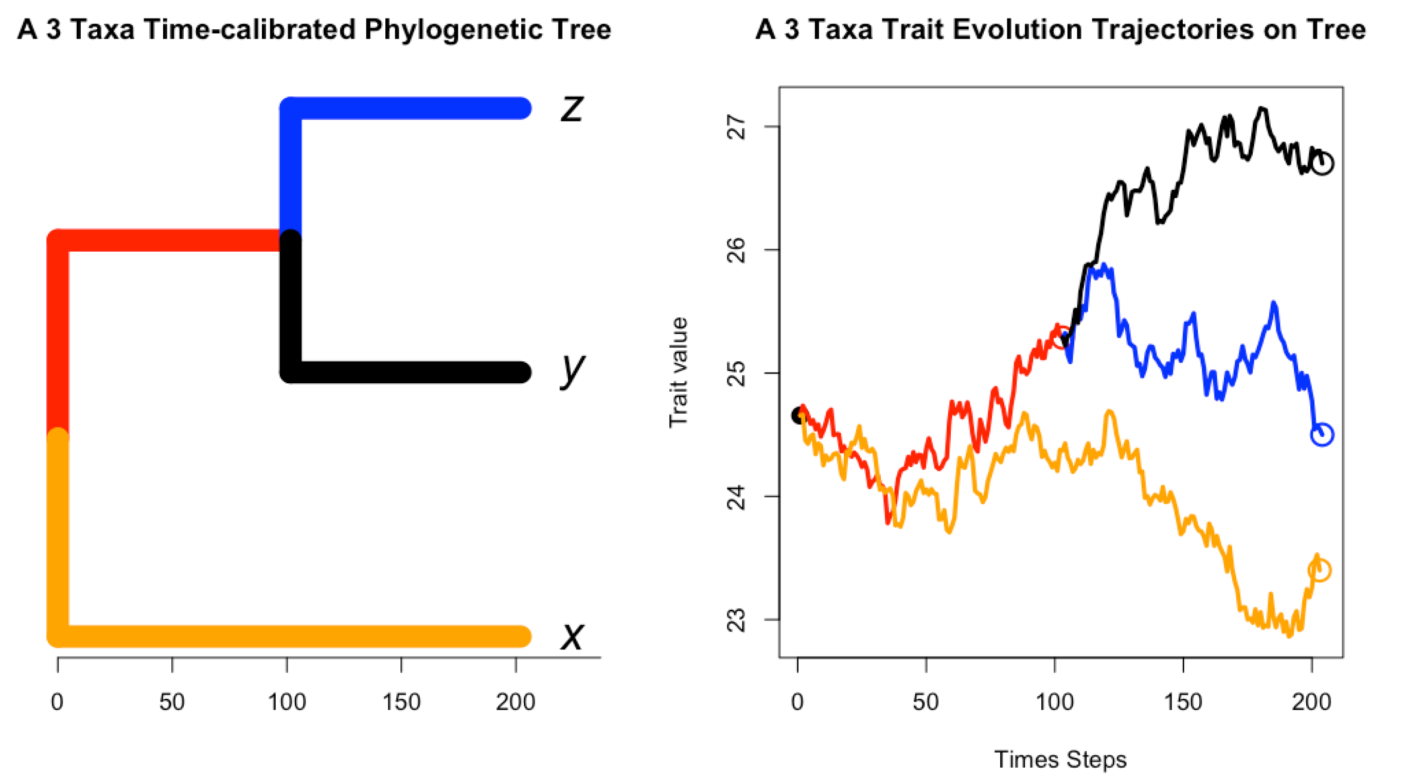
2.1. Gaussian Process for Trait Evolution along Tree

A Gaussian process is a collection of random variables indexed by time or space such that every finite set of these variables has a multivariate normal distribution. Let $x_t$ denote a Gaussian process variable. Its variance at any given time t is finite, that is, $\mathrm{var}\left[x\left(t\right)\right]=E\left[\right|x\left(t\right)-E\left[x\left(t\right)\right]{|}^2]<\infty$ for all $t\in T$. A key fact of Gaussian processes is that they are completely defined by their second-order statistics. This fact holds for Brownian motion, Ornstein-Uhlenbeck processes and the early burst process [16,17].

For single-trait evolution, a widely accepted assumption is that species share an evolutionary history modeled by a phylogenetic tree. The distribution of the trait variable of n species can be considered as a random vector $X={(x_1,x_2,\cdots ,x_n)}^t\in {\mathcal{R}}^n$, where $v^t$ denotes the transpose of a vector v. Under this evolutionary dependence is a multivariate distribution $X\sim {\mathcal{N}}_n(\mu 1_n,{\sigma }^2{\mathbf{\Sigma }}_{\mathrm{\Theta }})$ with mean vector $\mu 1_n$, where $1_n={(1,1,\cdots ,1)}^t$ is a vectors of 1s, and the symmetrical variance-covariance matrix ${\sigma }^2{\mathbf{\Sigma }}_{\mathrm{\Theta }}$ depends on the specific processes with parameter $\mathrm{\Theta }$ (see the following sections for more details). Here, $\mu$ is the common ancestor of the n species, $\sigma$ is the common rate of evolution, and ${\mathbf{\Sigma }}_{\mathrm{\Theta }}$ is the phylogenetic affinity matrix, with elements transformed from a given rooted phylogenetic tree with branch lengths and the corresponding model of stochastic processes (e.g., Brownian motion, Ornstein–Uhlenbeck process or early burst process) [18]. Note that a higher value of $\sigma$ results in a wider spread of traits, whereas a lower value indicates changes in traits within a narrower range. An example of a phylogenetic tree of three taxa, where each species adapted a dynamic Gaussian process along the tree, can be found in Figure 1.

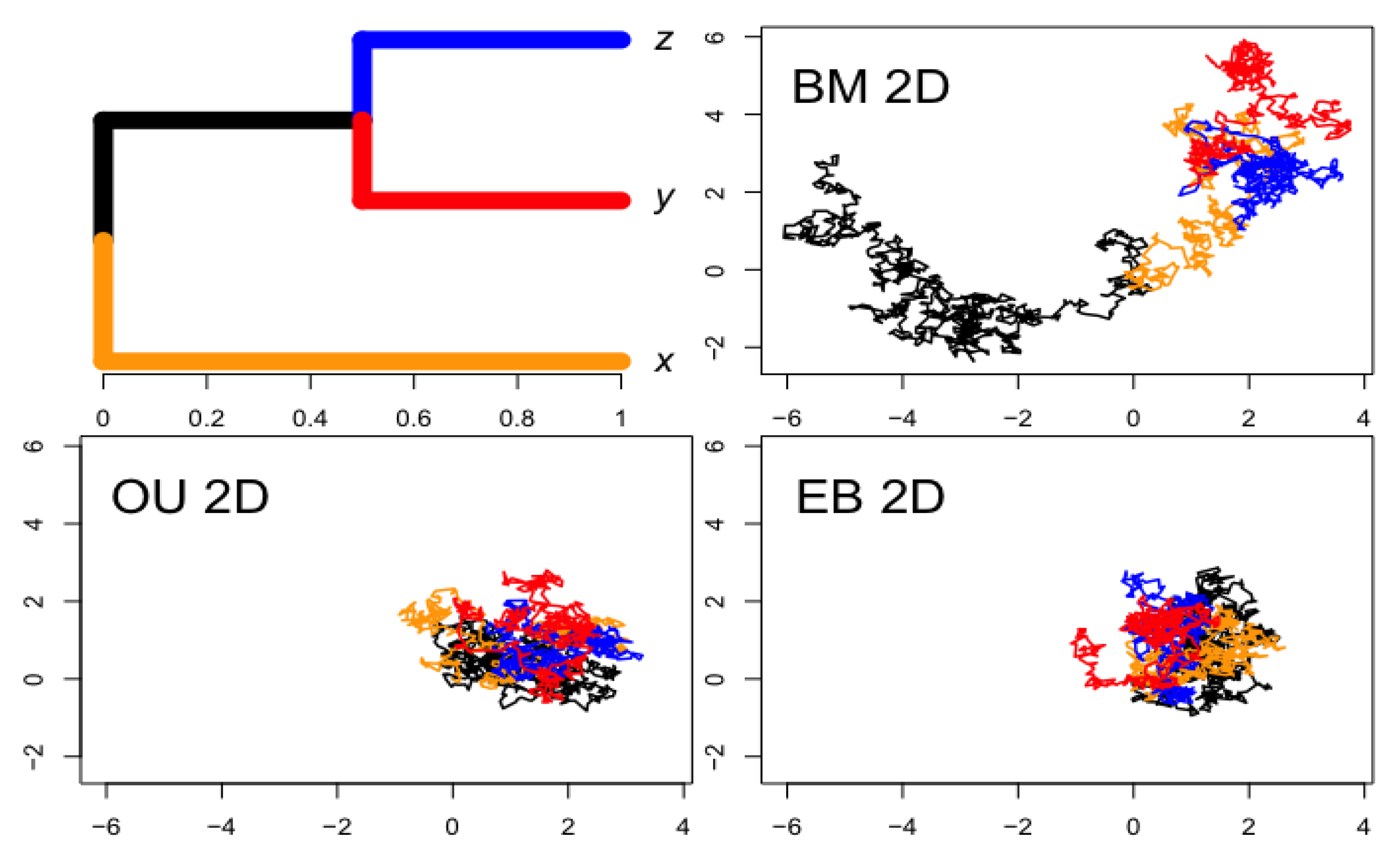
2.2. Statistical Model for Multiple Traits Evolution

When assessing the evolutionary rates of two or more phenotypic traits within a phylogenetic tree, the employment of a multivariate Gaussian model is necessary [19]. For characterizing multi-dimensional trait evolution within such a tree, a multivariate normal distribution model can be effectively applied. Let $\mathit{X}=(X_1,\cdots ,X_p)$ be an $n\times p$ data matrix containing p traits of n species. Let $X_u={(x_{u_1},x_{u_2},\cdots ,x_{u_n})}^t$ and $X_v={(x_{v_1},x_{v_2},\cdots ,x_{v_n})}^t$ be the uth and vth trait vectors. The covariances for $X_u$ and $X_v$, defined as ${\sigma }_{uv}$, measure the strength of impact from each other. In general, the variance-covariance matrix $\mathit{R}$ among the p traits can be defined as a matrix, as in Equation (1):

$$\mathit{R}=Cov[X_u,X_v]=\left[{\sigma }_{uv}\right].$$

(1)

Assuming a Gaussian process for trait evolution, the joint distribution of $\mathit{X}$ follows a matrix normal distribution (i.e., $\mathit{X}\sim {\mathcal{MN}}_{n\times p}(\mathit{M},\mathit{R},{\mathbf{\Sigma }}_{\mathrm{\Theta }})$), which is mathematically equivalent to the multivariate normal distribution, as illustrated in Equation (2):

$$\mathrm{vect}\left(\mathit{X}\right)\sim {\mathcal{N}}_{np}\left(\mathit{\mu },\mathit{R}\otimes {\mathbf{\Sigma }}_{\mathrm{\Theta }}\right),$$

(2)

where $\mathrm{vect}\left(\mathit{X}\right)\in {\mathcal{R}}^{np\times 1}$ is an $np\times 1$ random vector, $\mathit{\mu }={({\mu }_1{1}_n^t,{\mu }_2{1}_n^t,\cdots ,{\mu }_p{1}_n^t)}^t=E\left[\mathrm{vect}\left(\mathit{X}\right)\right]$ is the expected value of the random vector $\mathrm{vect}\left(\mathit{X}\right)$, and $\mathit{R}\otimes {\mathbf{\Sigma }}_{\mathrm{\Theta }}$ is an $np\times np$ variance covariance matrix where ⊗ is the tensor product operator.

Given trait data $\mathit{X}$, and a phylogenetic tree $\mathcal{T}$ with know topology and branch lengths, the negative log-likelihood function for the statistical model in Equation (2) is given by Equation (3):

$$\begin{array}{cc}-logL(\mathit{\mu },\mathit{R},{\mathbf{\Sigma }}_{\mathrm{\Theta }}|\mathit{X},\mathcal{T})\hfill & =\frac{pn}{2}log\left(2\pi \right)+\frac{1}{2}log|\mathit{R}\otimes {\mathbf{\Sigma }}_{\mathrm{\Theta }}|\hfill \\ & +\frac{1}{2}{(\mathrm{vect}\left(\mathit{X}\right)-\mathit{\mu })}^t{(\mathit{R}\otimes {\mathbf{\Sigma }}_{\mathrm{\Theta }})}^{-1}(\mathrm{vect}\left(\mathit{X}\right)-\mathit{\mu }),\hfill \end{array}$$

(3)

where $|\mathit{R}\otimes {\mathbf{\Sigma }}_{\mathrm{\Theta }}|$ denotes the determinant of the matrix $\mathit{R}\otimes {\mathbf{\Sigma }}_{\mathrm{\Theta }}$, and ${\mathbf{\Sigma }}_{\mathrm{\Theta }}^{-1}$ is the inverse of ${\mathbf{\Sigma }}_{\mathrm{\Theta }}$.

2.2.1. Multivariate Brownian Motion Model

Brownian motion has long been employed as a preferred continuous-time Markov process for modeling various biological phenomena, including trait evolution. The evolution of traits can be effectively captured by a Brownian motion variable, which is useful for representing both genetic drift and selection [14]. Consider the example shown in Figure 1, where the tree, scaled from root (at 0) to tip ($x,y,z$), spans a length of 200. For numerical convenience, we can rescale the tree to a tree height of 1. The species z and y share an evolutionary history of length $100/200=0.5$ (marked by the red horizontal line in Figure 1), leading to the assignment of $c_{zy}=c_{yz}=0.5$ in the matrix $\mathit{C}$. Since a species shares its entire history with itself, diagonal elements are assigned as $c_{xx}=c_{yy}=c_{zz}=200/200=1$. Species x, having no shared evolutionary history with z and y, results in elements $c_{zx}=c_{xz}=c_{yx}=c_{xy}=0$. The resultant matrix $\mathit{C}$ is detailed in Equation (4).

$$\mathit{C}=\begin{array}{cc}& \begin{array}{ccc}z& y& x\end{array}\\ \begin{array}{c}z\\ y\\ x\end{array}& \left[\begin{array}{ccc}1& 0.5& 0\\ 0.5& 1& 0\\ 0& 0& 1\end{array}\right]\end{array}$$

(4)

Here, $\mathit{C}$ represents a constant matrix derived from the phylogenetic tree, where each element within $\mathit{C}$ measures the length of the shared branch.

In the context of single-trait evolution within a group of n species, the trait vector $X={(x_1,x_2,\cdots ,x_n)}^t$ adheres to a multivariate normal distribution, symbolized as $X\sim {\mathcal{N}}_n(\mu 1_n,{\sigma }^2\mathit{C})$ (i.e., ${\mathbf{\Sigma }}_{\mathrm{\Theta }}=\mathit{C}$).

For multidimensional trait evolution on a phylogenetic tree, one can apply a multivariate Brownian diffusion (MBD) model [6]. Let $\mathit{X}=(X_1,\cdots ,X_p)$ represent an $n\times p$ data matrix that includes p traits of n species. The uth and the vth trait vectors are denoted as $X_u$ and $X_v$, respectively. The covariance for $X_u$ and $X_v$, denoted as ${\sigma }_{uv}$, measures the mutual influence of each trait on the other. Assuming Brownian motion for trait evolution, the joint distribution of $\mathit{X}\sim {\mathcal{MN}}_{n\times p}(\mathit{M},\mathit{R},\mathit{C})$ follows a matrix normal distribution [20,21], which is mathematically equivalent to the multivariate normal distribution, as illustrated in Equation (5):

$$\mathrm{vect}\left(\mathit{X}\right)\sim {\mathcal{N}}_{np}\left({\mathit{\mu }}_{bm},\mathit{R}\otimes \mathit{C}\right),$$

(5)

where ${\mathit{\mu }}_{bm}=E\left[\mathrm{vect}\left(\mathit{X}\right)\right]$ is the expected value of the $\mathrm{vect}\left(\mathit{X}\right)$, and for $i,j=1,2,\cdots ,n;$ $u,v=1,2,\cdots ,p,\mathrm{Cov}[X_{u_i},X_{v_j}]=\mathit{R}\otimes \mathit{C}[x_{u_i},x_{v_j}]$ can be expressed as

$$\mathit{R}\otimes \mathbf{\Sigma }[x_{u_i},x_{v_j}]={\sigma }_{x_u}{\sigma }_{x_v}{c}_{ij},$$

(6)

where with each block being an $n\times n$ matrix in an $np\times np$ block matrix $\mathit{R}\otimes \mathbf{\Sigma }$, the element ${\sigma }_{x_u}{\sigma }_{x_v}{c}_{ij}$ can be located in this block matrix at the intersection of the uth row block, the ith row, the vth column block, and the jth column.

The negative log-likelihood function is given by Equation (7):

$$\begin{array}{cc}-logL({\mathit{\mu }}_{bm},\mathit{R}|\mathit{X},\mathit{C})\hfill & =\frac{pn}{2}log\left(2\pi \right)+\frac{1}{2}log|\mathit{R}\otimes \mathit{C}|\hfill \\ & +\frac{1}{2}{(\mathrm{vect}\left(\mathit{X}\right)-{\mathit{\mu }}_{bm})}^t{(\mathit{R}\otimes \mathit{C})}^{-1}(\mathrm{vect}\left(\mathit{X}\right)-{\mathit{\mu }}_{bm}).\hfill \end{array}$$

(7)

2.2.2. Multivariate Ornstein–Uhlenbeck Model

Since the variation of trait change under Brownian motion is proportional to time, the trait may change without a reasonable bound, which cannot be a realistic situation in evolution (e.g., an ant weighing less than 5 mg is presumably unlikely to be able to evolve to a 3000 kg African elephant). Instead, one may consider that the species evolve in a more stable way, where traits shall evolve to an evolutionary peak and stay around it. Under this circumstance, another popular continuous-time Markov process, the Ornstein–Uhlenbeck (OU) process, was used to model the change in the trait [12,22]. Let $x_{it}$ denote a trait variable of the ith species observed at time t. If $x_{it}$ follows an OU process, a canonical representation for an OU variable $x_{it}$ using a diffusion equation is expressed in Equation (8).

$$d{x}_{it}=\alpha (\theta -x_{it})dt+\sigma d{W}_t,$$

(8)

where $\alpha$ is the force, $\theta$ is the optima, $\sigma$ is the rate of evolution, and $W_t$ is a Brownian motion variable. The deterministic form $\alpha (\theta -x_{it})$ in Equation (8) measures the quantity inherited from the previous generation in a relatively short time period $dt$, and the stochastic term $\sigma d{W}_t$ models random changes in the current environment [22]. Note that $x_{it}$ is expected to eventually move toward an optimum $\theta$ (the evolutionary niche). The selection force $\alpha$, under the OU process, is introduced to pull trait $x_{it}$ back to the optima $\theta$. For a stronger force (larger $\alpha$), $x_{it}$ moves at a faster tempo toward the optimum $\theta$, while a weak force (smaller $\alpha$) gradually pulls the trait to the optimum $\theta$. A special case is when $\alpha =0$: Equation (8) reduces to $d{x}_{it}=\sigma d{W}_t$, which is the diffusion process for a Brownian motion variable $x_{it}$.

For any $T>0$, $x_{it}=exp(-\alpha t)x_0+\theta (1-exp(-\alpha t))+\sigma {\int }_0^{T}exp\left(\alpha (T-s)\right)d{W}_s$ is a normal distribution with mean ${\mu }_{ou}=exp(-\alpha t)x_0+\theta (1-exp(-\alpha t))$ and variance ${\mathrm{\Sigma }}_{\alpha }={\sigma }^2(exp(2\alpha T-1))/\left(2\alpha \right)$ [22]. For a pair of species (species i and species j) evolved along a phylogenetic tree, under the OU process, the covariance matrix ${\sigma }^2{\mathbf{\Sigma }}_{\alpha }$ (i.e., ${\mathrm{\Sigma }}_{\mathrm{\Theta }}={\mathbf{\Sigma }}_{\alpha }$) has the following elements:

$${\mathbf{\Sigma }}_{\alpha }[i,j]=exp(-2\alpha (c_{ii}-c_{ij}))(1-exp(-2\alpha c_{ij}))/\left(2\alpha \right).$$

(9)

For instance, with $c_{zy}=0.5,c_{zz}=c_{yy}=1$, shown in Equation (4), can be expressed as $Cov[z,y]={\sigma }^2(exp(-2\alpha (1-0.5)))(1-exp(-2\alpha \times 0.5))/\left(2\alpha \right)$.

For single trait evolution on a phylogenetic tree $\mathcal{T}$, the trait vector X for n species follows a multivariate normal distribution $X\sim {\mathcal{N}}_n(\mu 1_n,{\sigma }^2{\mathbf{\Sigma }}_{\alpha })$.

For multidimensional trait evolution on a phylogenetic tree $\mathcal{T}$, the joint distribution of trait matrix $\mathit{X}\sim {\mathcal{MN}}_{n\times p}(\mathit{M},\mathit{R},{\mathbf{\Sigma }}_{\mathbf{\alpha }}),$ $\mathbf{\alpha }=({\alpha }_1,\cdots ,{\alpha }_p)$ follows a matrix normal distribution [13], which is mathematically equivalent to the multivariate normal distribution, as illustrated in Equation (10):

$$\mathrm{vect}\left(\mathit{X}\right)\sim {\mathcal{N}}_{np}\left({\mathit{\mu }}_{ou},\mathit{R}\otimes {\mathbf{\Sigma }}_{\mathbf{\alpha }}\right),$$

(10)

where ${\mathit{\mu }}_{ou}=E\left[\mathrm{vect}\left(\mathit{X}\right)\right]$ is the expected value of the $\mathrm{vect}\left(\mathit{X}\right)$, and for $i,j=1,2,\cdots ,n;$ $u,v=1,2,\cdots ,p,\mathrm{Cov}[X_{u_i},X_{v_j}]=\mathit{R}\otimes {\mathbf{\Sigma }}_{\mathbf{\alpha }}[x_{u_i},x_{v_j}]$ can be expressed as follows [13,23,24]:

$$\begin{array}{cc}\mathit{R}\otimes {\mathbf{\Sigma }}_{\mathbf{\alpha }}[x_{u_i},x_{v_j}]& ={\sigma }_{x_u}{\sigma }_{x_v}\frac{exp\left(-({\alpha }_u+{\alpha }_v)(c_{ii}-c_{ij})\right)\left(1-exp\left(-({\alpha }_u+{\alpha }_v)c_{ij}\right)\right)}{{\alpha }_u+{\alpha }_v}\end{array}$$

(11)

The negative log-likelihood function is given by Equation (12):

$$\begin{array}{cc}-logL({\mathit{\mu }}_{ou},{\mathbf{\Sigma }}_{\mathbf{\alpha }},\mathit{R}|\mathit{X},\mathit{C})\hfill & =\frac{pn}{2}log\left(2\pi \right)+\frac{1}{2}log|\mathit{R}\otimes {\mathbf{\Sigma }}_{\mathbf{\alpha }}|\hfill \\ & +\frac{1}{2}{(\mathrm{vect}\left(\mathit{X}\right)-{\mathit{\mu }}_{ou})}^t{(\mathit{R}\otimes {\mathbf{\Sigma }}_{\mathbf{\alpha }})}^{-1}(\mathrm{vect}\left(\mathit{X}\right)-{\mathit{\mu }}_{ou}).\hfill \end{array}$$

(12)

2.2.3. Multivariate Early Burst Model

An early burst model is useful for describing adaptive radiation, where species can evolve very quickly in relatively short periods to form many new species [14,25]. The finch species on the Galapagos Islands provide an example. The common ancestor of the finches was estimated to arrive on the Galapagos Islands about two million years ago and has now evolved into 15 species with different body sizes, beak shapes, songs, and feeding behaviors [26]. When modeling adaptive radiation under early burst process, it is assumed that the evolutionary rate ${\sigma }_t$ increases exponentially over a long time. One can describe ${\sigma }_t={\sigma }_{0}exp(\tau t/2)$, where ${\sigma }_0$ is the rate at the beginning of evolution, and $\tau <0$ is the parameter rate of decay of the rate. For a pair of species (e.g., green warbler finch and woodpecker finch [27]) evolved along a phylogenetic tree, under the EB process, their covariation relationship can be described by the covariance matrix ${\sigma }^2{\mathbf{\Sigma }}_{\tau }$ where

$${\mathrm{\Sigma }}_{\tau }[i,j]=(exp\left(\tau c_{ij}\right)-1)/\tau ,\tau <0.$$

(13)

For example, the covariance under the EB model between a pair of species z and y shown in Figure 2 is $Cov[z,y]={\sigma }^2(exp\left(0.5\tau \right))/\tau$. When using an early burst model for trait evolution, the trait vector X of n species follows a multivariate normal distribution with mean ${\mu }_{eb}=\mu$ and covariance ${\sigma }^2{\mathbf{\Sigma }}_{\mathrm{\Theta }}={\sigma }^2{\mathbf{\Sigma }}_{\tau }$ (i.e., $X\sim {\mathcal{N}}_n(\mu 1_n,{\sigma }^2{\mathbf{\Sigma }}_{\tau })$).

For studying a multi-trait case, the joint distribution of $\mathit{X}\sim {\mathcal{MN}}_{n\times p}(\mathit{M},\mathit{R},{\mathbf{\Sigma }}_{\mathbf{\tau }}),$ $\mathbf{\tau }=({\tau }_1,\cdots ,{\tau }_p)$ follows a matrix normal distribution, which is mathematically equivalent to the multivariate normal distribution, as illustrated in Equation (14):

$$\mathrm{vect}\left(\mathit{X}\right)\sim {\mathcal{N}}_{np}\left({\mathit{\mu }}_{eb},\mathit{R}\otimes {\mathbf{\Sigma }}_{\mathbf{\tau }}\right),$$

(14)

where ${\mathit{\mu }}_{eb}=E\left[\mathrm{vect}\left(\mathit{X}\right)\right]$ is the expected value of the $\mathrm{vect}\left(\mathit{X}\right)$, and for $i,j=1,2,\cdots ,n;$ $u,v=1,2,\cdots ,p,\mathrm{Cov}[X_{u_i},X_{v_j}]=\mathit{R}\otimes {\mathbf{\Sigma }}_{\mathbf{\tau }}[x_{u_i},x_{v_j}]$ can be expressed as

$$\mathit{R}\otimes {\mathbf{\Sigma }}_{\mathbf{\tau }}[x_{u_i},x_{v_j}]={\sigma }_{x_u}{\sigma }_{x_v}[exp(({\tau }_u+{\tau }_v)c_{ij}/2)-1].$$

(15)

The derivation of the covariance matrix $\mathit{R}\otimes {\mathbf{\Sigma }}_{\mathbf{\tau }}[i,j]$ is provided in Appendix A.2.1.

The negative log-likelihood function is given by Equation (16):

$$\begin{array}{cc}-logL({\mathit{\mu }}_{eb},{\mathbf{\Sigma }}_{\mathbf{\tau }},\mathit{R}|\mathit{X},\mathit{C})\hfill & =\frac{pn}{2}log\left(2\pi \right)+\frac{1}{2}log|\mathit{R}\otimes {\mathbf{\Sigma }}_{\mathbf{\tau }}|\hfill \\ & +\frac{1}{2}{(\mathrm{vect}\left(\mathit{X}\right)-{\mathit{\mu }}_{eb})}^t{(\mathit{R}\otimes {\mathbf{\Sigma }}_{\tau })}^{-1}(\mathrm{vect}\left(\mathit{X}\right)-{\mathit{\mu }}_{eb}).\hfill \end{array}$$

(16)

The evolution trajectories along a three-taxa phylogenetic tree in a two-dimensional Euclidean space under the Brownian motion model, the Ornstein–Uhlenbeck process models, and the early burst model are shown in Figure 2, respectively.

2.2.4. Multivariate Phylogenetic Mixed Model

The phylogenetic mixed model (PMM) is an application of the quantitative genetic mixed model to interspecific data, partitioning phenotypes into additive genetic (heritable) and non-heritable components [15]. The genetic component illustrates heritability, while the non-heritable partition corresponds to current environmental impacts and is independent of ancestors. A representative example of this phenomenon is the Daphnia species, which can develop helmets and beak teeth for protection in response to the presence of predators during growth, a trait not observed in other species.

Mathematically, the mixed model describes the trait phenotype ($x_i$ for the ith individual or ith taxon mean) as the sum of a grand mean ($\mu$), a heritable factor ($a_i$: from a normal distribution with a variance-covariance matrix ${\sigma }_a^2\mathit{C}$ (i.e., $a_i\sim \mathcal{N}(\mathbf{0},{\sigma }_a^2\mathit{C})$), and a residual deviation ($e_i$: independent normal variable with variance ${\sigma }_e^2$) [28] $x_i=\mu +a_i+e_i$, where the grand mean $\mu$ can be interpreted as the genotypic state of the ancestor at the root of a phylogeny in the phylogenetic context.

The PMM estimates the relative contribution of these two types of evolutionary change ($X\sim {\mathcal{N}}_n(\mu \mathbf{1},{\sigma }_a^2\mathit{C}+{\sigma }_e^2\mathit{I})$), where ${\sigma }_a^2$ and ${\sigma }_e^2$ are the variances for the heritable factor a and environmental factor e, respectively. However, fitting this model is challenging, possibly because the components of variance are confounded and cannot be estimated separately [28]. To overcome this, Ref. [15] recommended a re-parameterization of the model with total variance ${\sigma }^2={\sigma }_a^2+{\sigma }_e^2$ and a heritability factor $h^2={\sigma }_a^2/({\sigma }_a^2+{\sigma }_e^2),h^2\in [0,1]$, eliminating some of the difficulties, and developed a new estimation algorithm for both original maximum likelihood and new restricted maximum likelihood estimators. The correlation in the trait value between two species stems partially from the phylogenetic relationship between species (proportion $h^2$) and partially from an independent, species-specific contribution (proportion $1-h^2$). This forms a transformation to the original phylogeny that pictorially describes the correlation structure in the trait values between species. The statistical model for the PMM for a trait vector X follows a multivariate normal distribution with mean ${\mu }_{pmm}=\mu$ and covariance ${\sigma }^2{\mathrm{\Sigma }}_h$. For a pair of species $i,j$ evolved along a phylogenetic tree, the covariance matrix ${\mathrm{\Sigma }}_h$ has the following element:

$${\mathrm{\Sigma }}_h[i,j]=h^2{c}_{ij}+(1-h^2){\mathit{I}}_{ij},h\in [0,1].$$

(17)

The PMM provides rich evolutionary insights that can be drawn from its model parameters. It is worthwhile to discuss the interpretation of these parameters in a specific comparative analysis. When applying PMM for trait evolution, the trait vector X for n species follows a multivariate normal distribution $X\sim {\mathcal{N}}_n(\mu 1_n,{\sigma }^2{\mathbf{\Sigma }}_h)$.

For studying multi-trait cases, the joint distribution of $\mathit{X}\sim {\mathcal{MN}}_{n\times p}(\mathit{M},\mathit{R},{\mathbf{\Sigma }}_{\mathit{h}}),\mathit{h}=(h_1,\cdots ,h_p)$ follows a matrix normal distribution, which is mathematically equivalent to the multivariate normal distribution, as illustrated in Equation (18):

$$\mathrm{vect}\left(\mathit{X}\right)\sim {\mathcal{N}}_{n\times p}\left({\mathit{\mu }}_{pmm},\mathit{R}\otimes {\mathbf{\Sigma }}_{\mathit{h}}\right),$$

(18)

where ${\mathit{\mu }}_{pmm}=E\left[\mathrm{vect}\left(\mathit{X}\right)\right]$ is the expected value of the $\mathrm{vect}\left(\mathit{X}\right)$, and for $i,j=1,2,\cdots ,n;$ $u,v=1,2,\cdots ,p,\mathrm{Cov}[X_{u_i},X_{v_j}]=\mathit{R}\otimes {\mathbf{\Sigma }}_{\mathit{h}}[x_{u_i},x_{v_j}]$ can be expressed as

$$\mathit{R}\otimes {\mathbf{\Sigma }}_{\mathit{h}}[x_{u_i},x_{v_j}]={\sigma }_{x_u}{\sigma }_{x_v}\left(h_{uv}^2{c}_{ij}+(1-h_{uv}^2){\mathit{I}}_{ij}\right),h_{uv}\in [0,1].$$

(19)

The negative log-likelihood function is given by Equation (20):

$$\begin{array}{cc}-logL({\mathit{\mu }}_{pmm},{\mathbf{\Sigma }}_{\mathit{h}},\mathit{R}|\mathit{X},\mathit{C})\hfill & =\frac{pn}{2}log\left(2\pi \right)+\frac{1}{2}log|\mathit{R}\otimes {\mathbf{\Sigma }}_{\mathit{h}}|\hfill \\ & +\frac{1}{2}{(\mathrm{vect}\left(\mathit{X}\right)-{\mathit{\mu }}_{pmm})}^t{(\mathit{R}\otimes {\mathbf{\Sigma }}_{\mathit{h}})}^{-1}(\mathrm{vect}\left(\mathit{X}\right)-{\mathit{\mu }}_{pmm}).\hfill \end{array}$$

(20)

In the following, we provide a matrix decomposition to reduce the computational load from the inverse of $\mathit{V}$, ${\mathit{V}}^{-1}={(\mathit{R}\otimes {\mathbf{\Sigma }}_{\mathit{h}})}^{-1}$ by the following Lemma 1, which reduces the computation of the inverse of the $n^2\times n^2$ matrix into the inverse of the $n\times n$ matrices.

Lemma 1. 

Let $h\in [0,1]$ be the heritability parameter in the PMM model, and let the $n\times n$ matrix $\mathit{C}$ represent the affinity of the phylogenetic relationship for n taxa. Let $\mathit{R}$ be a $p\times p$ covariance matrix for p traits. Assuming all traits share the same heritability parameter h (i.e., $h_i=h$ for all $i=1,\cdots ,p,{\mathbf{\Sigma }}_{\mathit{h}}=h^2\mathit{C}+(1-h^2)\mathit{I}$), then

$${[\mathit{R}\otimes {\mathbf{\Sigma }}_{\mathit{h}}]}^{-1}=\frac{1}{2}{h}^{-2}{\mathit{R}}^{-1}\otimes {\mathit{C}}^{-1}[\mathit{I}-\frac{1-h^2}{h^2}\mathit{I}\otimes {\mathit{D}}_c^{-1}],$$

(21)

 where ⊗ is the tensor product operator, and ${\mathit{D}}_c$ is a diagonal matrix of eigenvalues of $\mathit{C}$.

The proof of Lemma 1 is provided in Appendix A.2.2.

3. Parameter Estimation and Testing

3.1. Estimation of the Rate Matrix and Compute the Likelihood

The rate matrix $\mathit{R}$ for multiple traits under the Brownian motion model can be analytically estimated using trait data ($\mathit{X}$) and the phylogenetic tree matrix ($\mathit{C}$). In this context, the covariance between the uth trait and vth trait in the BM model is ${\sigma }_{uv}\mathit{C}$. The rate matrix $\mathit{R}$ can be estimated as follows [11]:

$${\widehat{\mathit{R}}}_{bm}=\frac{(\mathit{X}-1_n{\mathit{\mu }}^t){\mathit{C}}^{-1}(\mathit{X}-1_n{\mathit{\mu }}^t)}{n-1},$$

(22)

where $\mathit{\mu }$ is the ancestral state vector at the root of the tree. The multivariate Brownian motion model thus provides a robust and efficient framework in a multivariate trait space [6].

Other models, such as the Ornstein–Uhlenbeck (OU), early burst (EB), and mixed phylogenetic model (PMM), incorporate an additional model parameter $\varphi$ in their covariance matrix, thus affecting the covariance of $\mathit{X}$. In particular, each trait i has its own parameters ${\mu }_i,{\sigma }_i,{\varphi }_i$, making the covariance of the traits u and v dependent on the parameters ${\varphi }_i$ and ${\varphi }_j$. In these cases, covariance in model $\mathcal{M}$ are generally represented as follows:

$${\mathit{R}}_{\mathcal{M}}=Cov[X_u,X_v|\mathit{C}]={\sigma }_u{\sigma }_v{\mathrm{\Sigma }}_{{\varphi }_u,{\varphi }_v}.$$

(23)

In our analysis, we utilize three different models to calculate covariance, with each one accompanied by a distinct set of parameters. The first model we employ is the Ornstein–Uhlenbeck (OU) model, which is delineated in Equation (11). The parameters for the OU model include ${\alpha }_u,{\alpha }_v>0$. These parameters are integral to the model, and the non-negative constants $c_{ii}$, $c_{ij}$ correspond to the elements of the covariance matrix. Next, we deploy the early burst (EB) model, which can be seen in Equation (15). Similar to the OU model, this model also uses the parameters ${\tau }_u,{\tau }_v<0$ as key components, with $c_{ii}$, $c_{ij}$ symbolizing the covariance matrix elements. Lastly, we incorporate the phylogenetic mixed model (PMM), as shown in Equation (19). Unlike the previous two models, this model uses $h_u,h_v\in [0,1]$ as heritability estimates as its unique set of parameters. The implementation of the covariance calculations for these models can be found in the code provided in Appendix A.1. For finding the maximum likelihood estimates, we utilize R version 4.2.3 software’s numerical optimization [29], as per the likelihood functions provided in Equation (12) for OU, Equation (16) for EB, and Equation (20) for PMM.

3.2. Compare the Fit of Models

Given tree data $\mathcal{T}$ with known topology and branch lengths and trait data $\mathit{X}$, all models considered use a Kronecker product covariance structure, denoted as $\mathit{R}\otimes {\mathbf{\Sigma }}_{\mathrm{\Theta }}$. Under the null hypothesis, the traits have the same rates. We apply the likelihood ratio test to assess the null hypothesis for each of the models under the BM, OU, EB, and PMM, specifically $H_0:{\sigma }_i^2={\sigma }_j^2$ vs. $H_1:{\sigma }_i^2\ne {\sigma }_j^2$. The test statistics are as follows:

$${\chi }^2=-2log\frac{L_{{\mathit{M}}_0}\left({\mathbf{\Theta }}_0\right|\mathit{X},\mathcal{T})}{L_{{\mathit{M}}_1}\left({\mathbf{\Theta }}_1\right|\mathit{X},\mathcal{T})},$$

(24)

which obey a chi-square distribution with degree of freedom $df=|{\mathrm{\Theta }}_1|-|{\mathrm{\Theta }}_0|$.

However, not all models are nested; for instance, the OU model, the EB model, and the PMM model are not nested to each other. Hence, to compare their fit to the data, we use the Akaike information criteria [30]: $\mathrm{AIC}=2k-2log{L}_{\mathit{M}}\left(\widehat{\mathbf{\Theta }}\right|\mathit{X},\mathcal{T})$, where k is the number of parameters, $log{L}_{\mathit{M}}$ is the negative log likelihood function under the model $\mathit{M}$, $\widehat{\mathbf{\Theta }}$ is the maximum likelihood estimator, $\mathit{X}$ is the trait matrix..The AICc is most suitable when the ratio between the sample size and the number of parameters is less than 40 (i.e., $n/k<40$, where n is taxa size). The AICc is calculated as follows:

$$\mathrm{AICc}=\mathrm{AIC}+2k(k+1)/(n-k+1).$$

(25)

4. Results

4.1. Simulation: Power Analysis

To evaluate the performance of the models, we use simulations to assess the statistical power. Two types of trees are used. The first type of tree is the balanced tree of taxa $16,32,64,128$ with Grafen branch, where the depth of each node of the tree is defined by the number of branching events above it [31]. The second type of tree uses the random split tree of taxa $25,50,80,120$ in ape 3.0 [32]. The root state is set to 0 for all models. Two sets of model-specific parameters are used for each model: for the OU model $({\alpha }_1,{\alpha }_2)=(0.2,0.2),(0.1,0.3)$; for the EB model $({\tau }_1,{\tau }_2)=(0.1,0.1),(0.05,0.2)$; for the PMM model $(h_1,h_2)=(0.5,0.5),(0.25,0.75)$. For each simulation, 1000 data sets are simulated for each type of tree, model, rate ratio, and taxa. For the analysis of statistical power under the null hypothesis and homogeneous rates between traits, the ratio of the two rates is set to ${\sigma }_2/{\sigma }_1\in \{1,1.5,2,3,4\}$, respectively.

Our analysis outcomes are presented in Figure 3. Consistent with the conventional understanding that statistical power increases with larger sample sizes, our results exhibit a similar pattern. A notable correlation is observed between the power and the ratio of two rates for the Brownian motion (BM) model, the early burst (EB) model, and the Ornstein–Uhlenbeck (OU) model. Interestingly, in the case of the phylogenetic mixed model (PMM), the power levels remain significantly high, unfazed by variations in the ratio of the two rates.

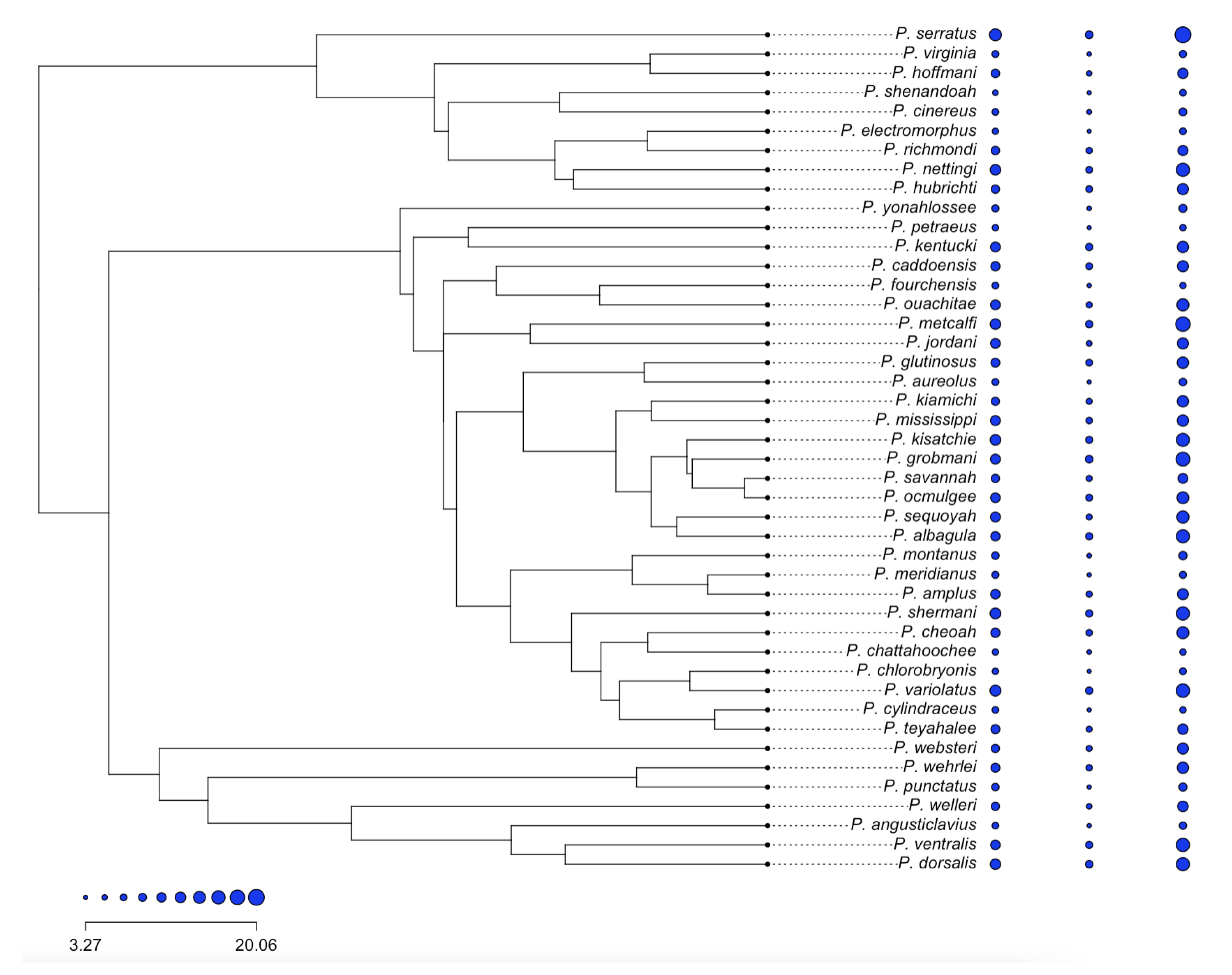
4.2. Empirical Study: Heterogeneous Rate of Evolution of the Salamander

Our analysis utilizes data sourced from [6], encompassing linear measurements for three phenotypic traits—head length, forelimb length, and body width—from 311 adult individuals. These individuals represent 44 out of the 45 known species of eastern Plethodon, as depicted in Figure 4. For each species, we computed the mean value for each trait. Given that all three traits were assessed in the same units (millimeters) and on the same scale, we employed the untransformed values in our analysis.

We frame our inquiry in the context of the following biological considerations [6,34,35]:

(i)

Head length: An increase in a creature’s head (and thereby, jaw) length is anticipated to enhance its biting strength and its proficiency in prey capture.

(ii)

Forelimb length: A longer forelimb is projected to augment the creature’s perceived body size during aggressive displays, possibly offering a competitive edge.

(iii)

Body width: Currently, there is no substantiated evidence indicating any impact of a creature’s body width on competitive behavior.

Given these considerations, it’s conceivable that the rate of evolution for body width may not align with that of the other traits. We will put our model to work, testing the heterogeneity in evolutionary rates between traits (i) and (iii) in Section 4.2.1, and then between traits (ii) and (iii) in Section 4.2.2, respectively.

4.2.1. Head Length vs. Body Width

Analyses of the comparison of head length and body width in salamanders are summarized in

Table 1. Summary of the results of the comparison of head length and body width in salamanders using four different phylogenetic models. The Obs (${\sigma }_H,{\sigma }_B$) represent the rate estimate under the alternative, while Con (${\sigma }_H,{\sigma }_B$) represents the rate estimate under the null hypothesis, where ${\sigma }_H,{\sigma }_B$ are the rate estimates for the head length and body width, respectively. $L_{obs}$ and $L_{con}$ are the log likelihood values, $LR{T}_{est}$ is the likelihood ratio test statistics, and $AIC{c}_{obs}$ and $AIC{c}_{con}$ are the sample size correct Akaike information criteria.

	BM	OU	PMM	EB
Obs (${\sigma }_H,{\sigma }_B$)	0.23, 0.13	0.23, 0.13	0.22, 0.13	0.23, 0.12
Con (${\sigma }_H,{\sigma }_B$)	1.02, 0.13	1.02, 0.16	1.02, 0.13	1.02, 0.13
$L_{obs}$	−126.85	−126.39	−126.82	−126.86
$L_{con}$	−188.32	−185.95	−187.82	−188.32
$LR{T}_{est}$	122.94	119.11	121.99	122.91
p-value	1.44 × ${10}^{-28}$	9.90 × ${10}^{-28}$	2.32 × ${10}^{-28}$	1.46 × ${10}^{-28}$
$AIC{c}_{obs}$	261.70	264.79	265.65	265.72
$AIC{c}_{con}$	382.63	381.90	385.64	386.63

.

The observed matrices (Obs) and constrained rate matrices (Con: under $H_0:{\sigma }_1={\sigma }_2$) exhibit variations across models, reflecting the differences in how each model estimates the relationship between head length and body width. This signifies the rejection of the null hypothesis. The likelihood of the observed data ($L_{obs}$) surpassed the likelihood of the constrained data ($L_{con}$). This indicates that the models potentially provide a superior fit to the observed data in comparison to the constrained data. Further validation of this observation is evident in the likelihood ratio test (LRT), revealing a significant positive relationship between head length and body width in salamanders across all models, as indicated by the notably low p-value. Moreover, the corrected Akaike information criterion (AICc) for the observed data was consistently lower than the AICc for the constrained data across all models, further suggesting that the models fit the observed data more effectively. These findings align with the outcomes of the study by [6], particularly in the context of a Brownian motion model.

4.2.2. Forelimb Length vs. Body Width

The results are summarized in

Table 2. Summary of the results of the comparison of body width and forelimb length in salamanders using four different phylogenetic models.

	BM	OU	PMM	EB
Obs (${\sigma }_B,{\sigma }_F$)	(0.12, 0.20)	(0.13, 0.21)	(0.13, 0.20)	(0.12, 0.20)
Con (${\sigma }_B,{\sigma }_F$)	(1.04, 0.20)	(1.05, 0.24)	(1.04, 0.21)	(1.01, 0.11)
$L_{obs}$	−134.21	−133.53	−134.25	−142.98
$L_{con}$	−193.43	-191.40	−192.87	−193.97
$LR{T}_{est}$	118.43	115.75	117.24	101.99
p-value	1.40 × ${10}^{-27}$	5.40 × ${10}^{-27}$	2.54 × ${10}^{-27}$	5.57 × ${10}^{-24}$
$AIC{c}_{obs}$	276.43	279.05	280.50	297.95
$AIC{c}_{con}$	392.85	392.80	395.74	397.95

.

Similarly to the previous analysis, for all models, the observed rate matrices (Obs) and constrained rate matrices (Con) varied between models, reflecting differences in the estimation of the relationship between body width and forelimb length in the different models. The likelihood of observed data ($L_{obs}$) was greater than the likelihood of constrained data ($L_{con}$), suggesting that the models fit the observed data better than they do the constrained data. Further validation of this observation is evident in the likelihood ratio test (LRT), revealing a significant positive relationship between forelimb length and body width in salamanders across all models, as indicated by the notably low p-value. The AICc for the observed data was less than the AICc for the constrained data across all models, suggesting that the models provide a better fit to the observed data.

4.3. Accessing Adequacy of Models via Many Empirical Datasets

Model adequacy refers to how well a statistical or mathematical model fits the data and underlying assumptions [36,37]. It evaluates whether the model’s assumptions are in line with the structure of the data and if the model sufficiently captures the patterns and relationships in the data. We use 9 trees and 221 empirical trait datasets, including a snow skinks group [38], Drosophila group [39], lizards group [40,41], woodcreepers group [42], sponges group [43], and bats group [44]. The aim is to minimize distinguishability, implying a higher adequacy of the model [36,37].

To achieve the aim, we first fit the model $\mathcal{M}$ to the raw dataset to obtain the maximum likelihood estimates (MLE) $\widehat{\mathrm{\Theta }}$ and compute the initial negative log-likelihood, ${\ell }_0$. Then, we simulate datasets using the model using $\widehat{\mathrm{\Theta }}$ and then compare these with observed datasets. We generate each simulated data set ${\mathit{X}}^{\prime }$ from estimates obtained from the empirical data under the model $\mathcal{M}$. We then compute the likelihood using $\widehat{\mathrm{\Theta }}$: ${\ell }^{\prime }:=-log{L}_{\mathcal{M}}\left({\mathit{X}}^{\prime }\right|\widehat{\mathrm{\Theta }},\mathit{C})$. If the normal distribution (as shown in this study) $\mathcal{M}$ is a candidate model, we can evaluate its adequacy by fitting the model $\mathcal{M}$ to the data ${\mathit{X}}^{\prime }$ to get the likelihood ${\ell }^{\prime }$ and as well as the MLE estimate for the parameter ${\widehat{\mathrm{\Theta }}}^{\prime }$ [45].

We simulate data ${\mathit{X}}_s^{\prime },s=1,\cdots ,B$ ($B=1000$) repeatedly using the MLE $\widehat{\mathrm{\Theta }}$ and compute the negative log-likelihood ${\ell }_s$. We then sort these results and find the relative location of the initial negative log-likelihood, ${\ell }_0$. If ${\ell }_0$ falls within the 90% limit of ${\ell }_s$, we can say that the data can be adequately analyzed by the model $\mathcal{M}$. The results are shown in Figure 5.

Figure 5 presents the evaluation of model adequacy, indicating that most datasets are appropriately analyzed using the proposed models. Specifically, the Brownian Motion (BM) model displays a higher degree of adequacy in comparison to other models, including the Ornstein-Uhlenbeck (OU), Phylogenetic Mixed Model (PMM), and Early Burst (EB). This measure of adequacy is determined by the likelihood calculated, even though this likelihood may exhibit substantial variations during the optimization search, particularly when the bootstrap samples are similar to the raw data.

We advise researchers to apply a cautious approach when utilizing these models in their analyses. It’s crucial to carry out an adequacy test to ensure that the data is effectively analyzed under the selected models. Nevertheless, it is worth noting that while the BM model showed the highest adequacy in our assessment, this does not devalue the applicability or potential usefulness of the other models, such as OU, PMM, and EB. Different models may be more appropriate depending on the specific characteristics of the data and research questions being addressed.

5. Discussion

The exploration of trait evolution has always been a crucial facet of evolutionary biology. It aids in the understanding of both the diversity and the adaptive mechanisms exhibited by different species. However, the traditional Brownian motion model, although providing valuable insights, does not fully capture the complexity and variability inherent in trait evolution across different species and traits. This limitation has prompted the need for more advanced models.

The current study has presented a robust step forward by introducing three extended statistical models: the phylogenetic multivariate Ornstein–Uhlenbeck model, the phylogenetic multivariate early burst model, and the phylogenetic multivariate mixed model. These models were found to provide a more nuanced perspective of trait evolution, fitting well to large datasets of varied traits in salamanders and lizards. Thus, these models appear promising for a wider range of studies in evolutionary biology.

Looking ahead, there are two major areas for future exploration. Firstly, there is room for refining the theoretical underpinnings of these models. This challenge involves the estimation and testing of models with a unique Kronecker product covariance structure. The traditional approaches such as the Taylor series, the convergence of the likelihood ratio, and the asymptotic power function could be adapted for this context. Testing of composite hypotheses, specifically in defining likelihood ratios under such hypotheses, presents another intriguing avenue of investigation. The aim is to simplify the computation and interpretation, thereby making these methods more accessible and applicable to a broader array of problems.

Secondly, a more comprehensive analysis of the work by [9], which builds on the methodology in [10], could prove to be valuable. We can use a likelihood-based approach to compare rates of phenotypic evolution for continuous traits across phylogenetic trees. While the model performs well, except in the case of very small trees, there is a need for refinement to minimize complexity and computational challenges, which presently limit its broad use. For example, it is known that a more efficient formulation to compute the likelihood using Equation (3) is given by $-logL(\mathit{\mu },\mathit{R},{\mathbf{\Sigma }}_{\mathrm{\Theta }}|\mathit{X},\mathcal{T})=\frac{pn}{2}log\left(2\pi \right)+\frac{n}{2}log\left|\mathit{R}\right|+\frac{p}{2}log\left|{\mathbf{\Sigma }}_{\mathrm{\Theta }}\right|+\frac{1}{2}\left(\mathrm{tr}\left({\mathit{R}}^{-1}{(\mathit{X}-E\left[\mathit{X}\right])}^t{\mathbf{\Sigma }}_{\mathrm{\Theta }}^{-1}(\mathit{X}-E\left[\mathit{X}\right])\right)\right)$, which reduce the cost of computing the $np\times np$ matrix to a $n\times n$ matrix, where $tr(·)$ denotes the trace of a square matrix. It remains a challenge for large tree cases (e.g., 100 taxa or more). Simplification, user-friendliness, optimizing algorithms such as the tree traversal algorithm [46] for the multivariate likelihood calculation, and intuitive interpretation are some of the aspects that need to be addressed.

Thirdly, while the primary focus has been centered around comparing rates among different models, however, it’s important to note that each model possesses unique functionalities that can be further explored. Thus, a deeper understanding of these models may necessitate individualized and detailed research projects. Specifically, a future area of investigation could involve interpreting the parameters of each model in the context of specific datasets. Such an approach might reveal nuanced insights and offer a more comprehensive view of each model’s capabilities and characteristics. This direction of research could provide significant contributions to the field.

Finally, in light of the research conducted by Baken et al. [47], Juarez and Adams [48], and Juarez et al. [49], we argue that implementing phylogenetic multivariate comparative methods could greatly enhance our understanding of evolutionary trends in salamanders. Future work should focus on improving theoretical understanding and developing practical tools that can investigate complex trait relationships, divergences, and the pace of evolution in relation to sexual dimorphism and microhabitat predilections across different species. These advanced models are a significant stride forward in the study of trait evolution, offering new insights into the rates of trait changes and heterogeneity across species and traits.

6. Conclusions

In this work, we proposed novel approaches, the multivariate phylogenetic early burst model and the multivariate phylogenetic mixed model, which serve to expand the toolbox available for understanding evolutionary processes. These models allow for a more nuanced and comprehensive investigation into trait covariance and evolution. Crucially, the results derived from these innovative models are consistent with those obtained through established models, namely the phylogenetic multivariate Brownian model [6] and the multivariate phylogenetic Ornstein–Uhlenbeck process model [13].

Our study presents a significant exploration into the evolution of three key organismal traits, head length, forelimb length, and body width, and their hypothesized impact on competitive behavior. We assert the plausibility of divergent rates of evolution for body width as compared to head length and forelimb length. Through our work, we apply and test this hypothesis using our newly developed multivariate phylogenetic models. This consistency not only validates our new methods but also reveals their utility and relevance in evolutionary studies.

In this way, our work serves to bridge the past and future of phylogenetic comparative methods, ensuring that our understanding of evolution is continually refined and improved upon. We believe these advancements will contribute to a more sophisticated comprehension of evolution’s intricate mechanisms, facilitating future research and discovery in this vital area of study.

References

1. Walsh, B.; Lynch, M. Evolution and Selection of Quantitative Traits; Oxford University Press: Oxford, UK, 2018. [Google Scholar]
2. Shankar, A.; Cisneros, I.N.; Thompson, S.; Graham, C.H.; Powers, D.R. A heterothermic spectrum in hummingbirds. J. Exp. Biol. 2022, 225, jeb243208. [Google Scholar] [CrossRef] [PubMed]
3. Rico-Guevara, A.; Hurme, K.J.; Rubega, M.A.; Cuban, D. Nectar feeding beyond the tongue: Hummingbirds drink using phase-shifted bill opening, flexible tongue flaps and wringing at the tips. J. Exp. Biol. 2023, 226, jeb245074. [Google Scholar] [CrossRef] [PubMed]
4. Piper, R. Extraordinary Animals: An Encyclopedia of Curious and Unusual Animals; Greenwood Press: London, UK, 2007; Volume 125. [Google Scholar]
5. Stebbins, R.C.; Cohen, N.W. A Natural History of Amphibians; Princeton University Press: Princeton, NJ, USA, 1997. [Google Scholar]
6. Adams, D.C. Comparing evolutionary rates for different phenotypic traits on a phylogeny using likelihood. Syst. Biol. 2013, 62, 181–192. [Google Scholar] [CrossRef] [PubMed]
7. Beaulieu, J.M.; Leitch, I.J.; Patel, S.; Pendharkar, A.; Knight, C.A. Genome size is a strong predictor of cell size and stomatal density in angiosperms. New Phytol. 2008, 179, 975–986. [Google Scholar] [CrossRef] [PubMed] [Green Version]
8. Beaulieu, J.M.; Jhwueng, D.C.; Boettiger, C.; O’Meara, B.C. Modeling stabilizing selection: Expanding the Ornstein–Uhlenbeck model of adaptive evolution. Evol. Int. J. Org. Evol. 2012, 66, 2369–2383. [Google Scholar] [CrossRef]
9. Revell, L.J.; González-Valenzuela, L.E.; Alfonso, A.; Castellanos-García, L.A.; Guarnizo, C.E.; Crawford, A.J. Comparing evolutionary rates between trees, clades and traits. Methods Ecol. Evol. 2018, 9, 994–1005. [Google Scholar] [CrossRef]
10. O’Meara, B.C.; Ané, C.; Sanderson, M.J.; Wainwright, P.C. Testing for different rates of continuous trait evolution using likelihood. Evolution 2006, 60, 922–933. [Google Scholar]
11. Adams, D.C.; Felice, R.N. Assessing trait covariation and morphological integration on phylogenies using evolutionary covariance matrices. PLoS ONE 2014, 9, e94335. [Google Scholar] [CrossRef] [Green Version]
12. Hansen, T.F. Stabilizing selection and the comparative analysis of adaptation. Evolution 1997, 51, 1341–1351. [Google Scholar] [CrossRef]
13. Bartoszek, K.; Pienaar, J.; Mostad, P.; Andersson, S.; Hansen, T.F. A phylogenetic comparative method for studying multivariate adaptation. J. Theor. Biol. 2012, 314, 204–215. [Google Scholar] [CrossRef]
14. Harmon, L. Phylogenetic Comparative Methods: Learning from Trees; CreateSpace Independent Publishing Platform: Scotts Valley, CA, USA, 2018. [Google Scholar]
15. Housworth, E.A.; Martins, E.P.; Lynch, M. The phylogenetic mixed model. Am. Nat. 2004, 163, 84–96. [Google Scholar] [CrossRef] [Green Version]
16. Nelson, E. Dynamical Theories of Brownian Motion; Princeton University Press: Princeton, NJ, USA, 2020; Volume 101. [Google Scholar]
17. Gramacy, R.B. Surrogates: Gaussian Process Modeling, Design, and Optimization for the Applied Sciences; Chapman and Hall/CRC: Boca Raton, FL, USA, 2020. [Google Scholar]
18. Jhwueng, D.C.; O’Meara, B.C. On the Matrix Condition of Phylogenetic Tree. Evol. Bioinform. 2020, 16, 1176934320901721. [Google Scholar] [CrossRef]
19. Hsu, M.H. Studying Rate of Evolution in Multi Dimensional Trait Space. Master’s Thesis, Feng-Chia University, Taichung, Taiwan, 2022. [Google Scholar]
20. Adams, D.C.; Collyer, M.L. Multivariate phylogenetic comparative methods: Evaluations, comparisons, and recommendations. Syst. Biol. 2018, 67, 14–31. [Google Scholar] [CrossRef]
21. Hassler, G.; Tolkoff, M.R.; Allen, W.L.; Ho, L.S.T.; Lemey, P.; Suchard, M.A. Inferring phenotypic trait evolution on large trees with many incomplete measurements. J. Am. Stat. Assoc. 2020, 117, 678–692. [Google Scholar] [CrossRef]
22. Butler, M.A.; King, A.A. Phylogenetic comparative analysis: A modeling approach for adaptive evolution. Am. Nat. 2004, 164, 683–695. [Google Scholar] [CrossRef]
23. Blomberg, S.P.; Garland, T., Jr.; Ives, A.R. Testing for phylogenetic signal in comparative data: Behavioral traits are more labile. Evolution 2003, 57, 717–745. [Google Scholar]
24. Jhwueng, D. Some Problems in Phylogenetic Comparative Method. Ph.D. Thesis, Indiana University Bloomington, Bloomington, IN, USA, 2010. [Google Scholar]
25. Puttick, M. Mixed evidence for early bursts of morphological evolution in extant clades. J. Evol. Biol. 2018, 31, 502–515. [Google Scholar] [CrossRef] [Green Version]
26. Grant, P.R. Ecology and Evolution of Darwin’s Finches; Princeton Science Library Edition; Princeton University Press: Princeton, NJ, USA, 2017. [Google Scholar]
27. Burns, K.J.; Hackett, S.J.; Klein, N.K. Phylogenetic relationships and morphological diversity in Darwin’s finches and their relatives. Evolution 2002, 56, 1240–1252. [Google Scholar]
28. Paradis, E. Analysis of Phylogenetics and Evolution with R; Springer Science & Business Media: New York, NY, USA, 2011. [Google Scholar]
29. R Core Team. R: 4.2.3 A Language and Environment for Statistical Computing; R Foundation for Statistical Computing: Vienna, Austria, 2023. [Google Scholar]
30. Anderson, D.; Burnham, K. Model Selection and Multi-Model Inference, 2nd ed.; Springer: New York, NY, USA, 2004; Volume 63, p. 10. [Google Scholar]
31. Grafen, A. The phylogenetic regression. Philos. Trans. R. Soc. Lond. B Biol. Sci. 1989, 326, 119–157. [Google Scholar]
32. Popescu, A.A.; Huber, K.T.; Paradis, E. ape 3.0: New tools for distance-based phylogenetics and evolutionary analysis in R. Bioinformatics 2012, 28, 1536–1537. [Google Scholar] [CrossRef] [Green Version]
33. Kumar, S.; Stecher, G.; Suleski, M.; Hedges, S.B. TimeTree: A resource for timelines, timetrees, and divergence times. Mol. Biol. Evol. 2017, 34, 1812–1819. [Google Scholar] [CrossRef] [PubMed]
34. Adams, D.C.; Berns, C.M.; Kozak, K.H.; Wiens, J.J. Are rates of species diversification correlated with rates of morphological evolution? Proc. R. Soc. B Biol. Sci. 2009, 276, 2729–2738. [Google Scholar] [CrossRef] [PubMed]
35. Adams, D.C. Quantifying and comparing phylogenetic evolutionary rates for shape and other high-dimensional phenotypic data. Syst. Biol. 2014, 63, 166–177. [Google Scholar] [CrossRef] [PubMed] [Green Version]
36. Beaulieu, J.M.; O’Meara, B.C. Detecting hidden diversification shifts in models of trait-dependent speciation and extinction. Syst. Biol. 2016, 65, 583–601. [Google Scholar] [CrossRef] [PubMed] [Green Version]
37. Stern, D.B.; Breinholt, J.; Pedraza-Lara, C.; López-Mejía, M.; Owen, C.L.; Bracken-Grissom, H.; Fetzner, J.W., Jr.; Crandall, K.A. Phylogenetic evidence from freshwater crayfishes that cave adaptation is not an evolutionary dead-end. Evolution 2017, 71, 2522–2532. [Google Scholar] [CrossRef] [Green Version]
38. Melville, J.; Swain, R. Evolutionary correlations between escape behaviour and performance ability in eight species of snow skinks (Niveoscincus: Lygosominae) from Tasmania. J. Zool. 2003, 261, 79–89. [Google Scholar] [CrossRef]
39. Moreeteau, B.; Gibert, P.; Pétavy, G.; Morteau, J.C.; Huey, R.; David, J. Morphometrical evolution in a Drosophila clade: The Drosophila obscura group. J. Zool. Syst. Evol. Res. 2003, 41, 64–71. [Google Scholar] [CrossRef] [Green Version]
40. Bonine, K.E.; Gleeson, T.T.; Garland, T., Jr. Muscle fiber-type variation in lizards (Squamata) and phylogenetic reconstruction of hypothesized ancestral states. J. Exp. Biol. 2005, 208, 4529–4547. [Google Scholar] [CrossRef] [Green Version]
41. Vanhooydonck, B.; Van Damme, R.; Aerts, P. Variation in speed, gait characteristics and microhabitat use in lacertid lizards. J. Exp. Biol. 2002, 205, 1037–1046. [Google Scholar] [CrossRef]
42. Tubaro, P.L.; Lijtmaer, D.A.; Palacios, M.G.; Kopuchian, C. Adaptive modification of tail structure in relation to body mass and buckling in woodcreepers. Condor 2002, 104, 281–296. [Google Scholar] [CrossRef]
43. Sanchez, J.A.; Lasker, H.R. Patterns of morphological integration in marine modular organisms: Supra-module organization in branching octocoral colonies. Proc. R. Soc. Lond. Ser. B Biol. Sci. 2003, 270, 2039–2044. [Google Scholar] [CrossRef]
44. Aguirre, L.F.; Herrel, A.; Van Damme, R.; Matthysen, E. Ecomorphological analysis of trophic niche partitioning in a tropical savannah bat community. Proc. R. Soc. Lond. Ser. B Biol. Sci. 2002, 269, 1271–1278. [Google Scholar] [CrossRef]
45. Rice, A.; Mayrose, I. Model adequacy tests for probabilistic models of chromosome-number evolution. New Phytol. 2021, 229, 3602–3613. [Google Scholar] [CrossRef]
46. Tung Ho, L.s.; Ané, C. A linear-time algorithm for Gaussian and non-Gaussian trait evolution models. Syst. Biol. 2014, 63, 397–408. [Google Scholar] [CrossRef]
47. Baken, E.K.; Mellenthin, L.E.; Adams, D.C. Is salamander arboreality limited by broad-scale climatic conditions? PLoS ONE 2021, 16, e0255393. [Google Scholar] [CrossRef]
48. Juarez, B.H.; Adams, D.C. Evolutionary allometry of sexual dimorphism of jumping performance in anurans. Evol. Ecol. 2022, 36, 717–733. [Google Scholar] [CrossRef]
49. Juarez, B.H.; Moen, D.S.; Adams, D.C. Ecology, sexual dimorphism, and jumping evolution in anurans. J. Evol. Biol. 2023, 36, 829–841. [Google Scholar] [CrossRef]
50. Higham, N.J. Accuracy and Stability of Numerical Algorithms; SIAM: Philadelphia, PA, USA, 2002. [Google Scholar]
51. AmphibiaWeb. 2023. Available online: https://amphibiaweb.org/ (accessed on 10 July 2023).
Figure 1. (Left) A phylogenetic tree illustrating the evolutionary relationships among three species x , y , and z, originating from a common root. (Right) Depiction of evolutionary trait trajectories derived from a Brownian process, progressing along the structure of the tree. Each color on each branch represents the evolutionary trajectories. The circle in black at time t = 0 is the root node, the circle in red at time t = 105 is the ancestral node, and the circles in black, blue, and orange are the tip nodes at t = 200 .
Symmetry 15 01445 g001
Figure 2. This figure presents the evolutionary trajectories of three species in a two-dimensional trait space. The top left shows the phylogenetic tree of the species. The remaining panels simulate trajectories under different models: Brownian motion (BM) at top right, Ornstein–Uhlenbeck (OU) at bottom left, and early burst (EB) at bottom right. All models start from the origin with zero covariation and specific parameters: for BM and OU, rates are set at σ 1 = σ 2 = 0.1 ; for OU, force parameters are α 1 = α 2 = 0.01 and optimal parameters are θ 1 = θ 2 = 1 ; and for EB, decay parameters are τ 1 = τ 2 = 0.18 .
Symmetry 15 01445 g002
Figure 3. Statistical power for BM, PMM, EB, and OU models. Taxa 16, 32, 64, and 128 are shown in black, blue, red, and purple, respectively.
Symmetry 15 01445 g003
Figure 4. This phylogenetic tree represents 44 salamander species, based on data reproduced via the TimeTrees tool as outlined by [33]. The species names used align with those provided in [6]. With the evolutionary timescale extending from the root to the tip covering approximately 25.41 million years, the tree helps in examining and analyzing the evolution of certain traits over time. Specifically, the traits of interest in this context are head length, body width, and forelimb, which will be used for later analysis.
Symmetry 15 01445 g004
Figure 5. Assessing model adequacy using the empirical dataset. A total of 9 trees and 221 trait sets are used. Each point in the subfigure represents the quantify of the maximum likelihood of the raw dataset computed by the log L M ( Θ ^ | X , C ) concerning the maximum likelihood of the simulated data log L M ( X s | Θ ^ , C ) , s = 1 , 2 , , 1000 . The two horizontal lines are the 90% cut-off quantile.
Symmetry 15 01445 g005