1. Introduction
In a series of works [
1,
2], it has been shown that the use of a device with circular rings carrying electric currents of the same intensity but in a random flow direction results in a symmetrical stratified magnetic field, i.e., a magnetic field that presents a zonal structure around an axis of symmetry. Furthermore, using the most recently introduced prime-numbers-based algorithm (PNA) to simulate the magnetic field of the specific device [
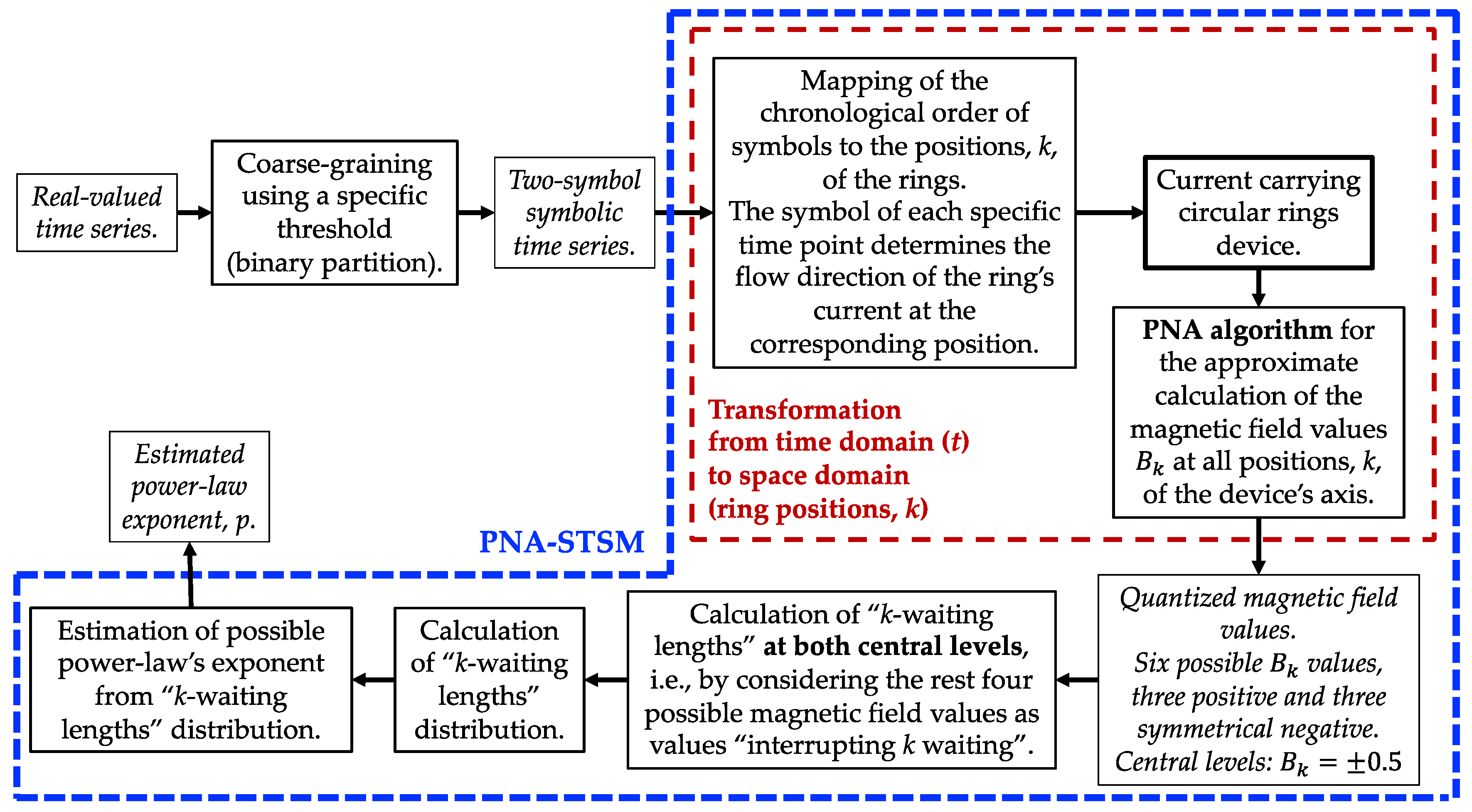
3], the quantization of the above-mentioned stratified magnetic field is achieved, i.e., the magnetic field values’ zones can be converted to quantized magnetic field values. Thus, if a two-symbol symbolic time series (using, for example, the symbols “+1”, “−1”) is employed to determine the flow directions of the rings’ currents, a time-to-space mapping of the dynamics of the system producing the time series, is achieved [
3]. This mapping enables the calculation of the exponents of the “waiting times” distributions in the space of the magnetic field positions, “
” leading to the development of the method of symbolic time-series analysis referred to as the PNA-based symbolic-time-series-analysis method (PNA-STSM) [
3]). The PNA-STSM can be applied to any two-symbol symbolic time series that is produced directly or indirectly (after coarse-graining) by any real or numerical dynamic system and presents the advantage that it can reliably expose the real dynamics of a complex system, even if a relatively short time series is available and the probabilities of the occurrence of each of the two symbols are not equal [
3].
Waiting times are essential because their distribution can reveal the dynamics of the system generating the time series under analysis [
3]. For example, if the distribution of the waiting times follows a power law with the exponent
p this is a strong indication that the system is in its critical state [
4]. On the other end of the dynamical spectrum, the presence of exponential laws in these distributions suggests the complete absence of dynamics that create long scales; in such cases, long scales are truncated [
5]. Between these two extremes of the dynamics spectrum, any intermediate state can be quantitatively determined from the competition of these two extreme cases (power law and exponential distributions).
Furthermore, waiting times can be defined in different ways. For example, in time series resulting from intermittent dynamics, the waiting times, also called laminar lengths [
6], are defined as the time intervals between bursts, namely, the number of consecutive values of the time series that fall within specific thresholds that define the boundaries of a non-burst (laminar) values’ region. In a sequence of symbols, such as the symbolic dynamics of the symbols “+1” and “−1”, the waiting times are defined as the number of the same consecutive symbols (e.g., “+1”), which are interrupted by a number of consecutive appearances of the other symbol (e.g., “−1”), or vice versa. A key difference from the above-mentioned time domain (waiting-time-based) analysis approaches is that PNA-STSM introduces a space-domain analog of waiting times, called “
waiting lengths,” which takes into account both symbols’ dynamics.
The first part of this work shows that PNA-STSM is an analysis method capable of correctly estimating the exponents characterizing the dynamics embedded in a time series. This is proven by comparing the results obtained by PNA-STSM with the results obtained by other well-known and reliable methods, as well as with the theoretical results for the 3D Ising model in the critical state. Subsequently, the main advantages of PNA-STSM over other analysis methods are highlighted. Three examples of dynamical systems are employed to demonstrate the efficacy of PNA-STSM. The first is a numerical example and refers to a special behavior of the 3D Ising model, and the second is from the area of nano-electronics, and the third concerns earthquake (EQ)-preparation processes. The common behaviors of these three systems are that they all obey the dynamics of on–off intermittency (of various forms) and that they all present bimodal (two-lobe) amplitude distributions, which, as has recently been shown [
7], appears to be connected with the spontaneous symmetry breaking (SSB) phenomenon observed in the preparation of the second-order phase transition in finite systems. Through these examples, it is shown how to apply the PNA-STSM to systems that obey the dynamics of on–off intermittency and present bimodal amplitude distributions in order to extract the information on their critical state and the SSB. Moreover, it is demonstrated that beyond on–off intermittency, PNA-STSM can provide credible results for the dynamics of any two-symbol symbolic-dynamics time series or for general two-symbol sequences because it is not affected by any imbalances in the probability of the appearance of the two symbols, since it simultaneously considers the information from both branches of the symbolic dynamics.
2. The 3D Ising Model and Its Waiting Times
The 3D Ising model is a well-known model in statistical mechanics describing specific ferromagnetic behavior [
8,
9]. It successfully describes the continuous phase transition in equilibrium, as well as more specialized topics, such as the SSB of the
Landau free energy [
10]. According to the theory of critical phenomena, all natural systems are classified into universality classes that are characterized by the values of the so-called critical exponents. The 1D Ising model has been analytically solved by Ernst Ising [
11] and does not present phase transition for any finite temperature. Likewise, the 2D Ising model has been analytically solved by Onsager [
12], and the six critical exponents of this model have been accurately calculated. Finally, the 3D Ising model has not been solved analytically yet, but only numerical solutions have been provided. However, it must be mentioned that in [
13], and under suitable boundary conditions, the 3D Ising model can be described by the operator algebra and thus can be solved exactly. This theory has been studied using renormalization group methods, Monte-Carlo simulations, conformal bootstrap and other techniques [
8,
9,
14,
15].
Generally speaking, for a Z(N) spin system, spin variables are defined as:
(lattice vertices
), with
. For
, one may derive the above-mentioned Ising models. Utilizing the Metropolis algorithm configurations at constant temperatures may be selected with Boltzmann statistical weights
, where
is the Hamiltonian of the spin system for which the nearest neighbors’ interactions without external field can be written as:
It is known that this model undergoes a second-order phase transition when the temperature drops below a critical value [
10,
16]. Thus, for a lattice of
nodes in three dimensions (3D Ising model), the critical (or pseudocritical for finite-size lattices) temperature has been found to be
(
1). Considering the sweep of the whole lattice as an algorithmic time unit, the possible values that spin can have in the model are ±1. The quantity recorded in a numerical experiment (conducted using the Metropolis algorithm) is the mean magnetization (space averaged magnetization density)
, which plays the role of the order parameter. The trajectory generated by the numerical experiment is a “time series” of the fluctuations of the order parameter. This means that for a simulation performed for
lattice sweeps, the generated time series of
will consist of
-points, with a time step equal to the algorithmic time of the whole lattice sweep.
Figure 1 presents the distribution of the resulting mean magnetization
values at the pseudocritical point
for
.
Calculating the distribution of waiting times (see
Section 1), one may extract useful and important quantitative information about the dynamics of the studied system. In the cases that this distribution turns out to be a scale-free function (i.e., a power law), the signature of the critical state of the system could be revealed. Therefore, the correct calculation of waiting times is of great importance. As it has been shown in [
4,
17], the fluctuations of the order parameter at the critical point follow the dynamics of Type I intermittency, for which it is known that the distribution
of the appropriately defined waiting times
(laminar lengths, see
Section 1) follows a power law of the form [
6]:
As shown in [
4], the exponent
is related to the isothermal critical exponent
, as:
while it holds that
[
4], where
is the effective action for the mean magnetization. It is also mentioned that the exponent
is related to other well-known exponents through the isothermal critical exponent
(one of the six critical exponents, related one another through four relations, known as “scaling laws” [
16]). Moreover, it has been shown that
is related to the spectral exponent, the Hurst exponent, and the fractal dimension [
18], as well as to the exponent describing Lévy flights and the Tsallis non-extensive parameter
[
19].
Since
[
16], one may deduce from Equation (3) that the critical state exists when
. Beyond the critical point, another type of intermittency dynamics [
20] that describe the dynamics of the order parameter fluctuations at the beginning of a tricritical crossover, has been found. This happens around the point where the second-order phase transition and the first-order phase transition lines meet in the parametric space of Ginzburg–Landau free energy (tricritical point according to Griffiths [
16]). In this case, the exponent
of the power law distribution of laminar lengths is given as [
4]:
from which it follows that
[
21]. At this point, it should be mentioned that when the distribution of the waiting times follows a power law with an exponent
it probably refers to some subcritical region without clear boundaries that can be predicted by the theory, and it does not indicate criticality (critical or tricritical point). In our analyses of dynamical systems, real and numerical, coming from different disciplines, we have not yet come across such a case.
In [
4], the value of the exponent
for the critical 3D Ising model has been estimated with very good agreement with the one predicted from the theory of critical phenomena, using the notion of waiting times in a time series (see
Section 1). Specifically, using the method of critical fluctuations (MCF) [
4,
22], which has been introduced for this purpose, it has been found that the exponent
obtains the value
for the critical 3D Ising model [
4]. Exactly at the pseudocritical point, the characteristic exponent is the isothermal critical exponent
. Notice that for the 3D Ising model this exponent has the value
[
23]. Consequently, from Equation (4), the theoretical value of the exponent
is
, and therefore, the value estimated using the MCF for the numerical experiment (
) is in perfect agreement with the theoretical one.
Another way to calculate the exponent
of the distribution of the waiting times in the critical 3D Ising model is to resort to symbolic dynamics based on two symbols in the time domain. This can be achieved by appropriately converting the mean magnetization time series to a symbolic time series and then by defining the waiting times as the number of the same consecutive symbols (see
Section 1). Given that the distribution of
Figure 1 is almost symmetrical around
, a straightforward way to obtain a two-state coarse-graining description of the mean magnetization value for the specific numerical experiment (as mentioned, 200,000 configurations of a
3D Ising lattice at the pseudocritical temperature
) is to assign positive and negative time series values to the symbols “+1” and “−1”, respectively. Thus, the simulated mean magnetization time series is converted into a two-symbol symbolic time series. By calculating the waiting times of the obtained mean magnetization symbolic time series, one may create the distributions for each of the two symbols, which are shown in
Figure 2. As in the MCF, one may employ the truncated power law function
for each symbol in order to model the distribution of waiting times
:
In the case that
, then
is equal to the power law exponent
.
For the waiting times corresponding to the symbol “+1”, their distribution indeed follows a power law with an exponent value
(
Figure 2a); while for the waiting times corresponding to the symbol “−1”, again a power law distribution holds, but this time with a different exponent value of
(
Figure 2b). Apparently, these exponent values are not the same due to the small asymmetry between the two symbols, 49% (“+1”’s) vs. 51% (“−1”’s) probability of occurrence, which is reflecting the small asymmetry between the positive and negative values of the original mean magnetization time series (also 49% vs. 51%, see the distribution in
Figure 1). It is also noted that considering the error limits, the “+1” branch leads to
values in the range between 1.142 and 1.176, while the “−1” branch leads to
values in the range between 1.156 and 1.208, which intersect one another. However, the resulting higher value for the “+1” branch (1.176) is close but lower than the nominal value of the “−1” branch (1.182). Thus, one cannot claim that the two nominal values (1.159 and 1.182) coincide within their error limits.
Summing up, based on the same numerical data of 200,000 configurations for a
lattice at the pseudocritical temperature
, the MCF estimates for the exponent
a value of 1.21, whereas the waiting times analysis of the corresponding two-symbol symbolic time series in the time domain leads to two different exponent
values, 1.159 and 1.182, for each symbolic branch; while we know that for the 3D Ising model, the theoretically calculated value of the waiting times distribution’s power law exponent is
. From the above, it is clear that although the existence of dynamics in a 3D Ising two-symbol symbolic time series can be revealed in the time domain via the scaling behavior of the waiting times, the quantitative result is ambiguous, even for time series with only a slight asymmetry in the distribution of their values, as has also been shown in [
3] for the case of the 2D Ising model. Furthermore, the 3D Ising model case proves that this result is not only ambiguous but also far from the one theoretically calculated. However, it has been proven in [
3] that PNA-STSM can overcome this ambiguity issue, even for time series of relatively short length, in which one of the symbols appears more often than the other. So, in
Section 3, after a brief presentation of the key notions of the PNA-STSM, the case of the 3D Ising symbolic time series is analyzed using the PNA-STSM, leading not only to unambiguous but also accurate exponent
estimation.
4. Analysis of Time Series Presenting Two-Lobes’ Amplitude Distributions Using PNA-STSM
As has recently been shown [
7,
24] and according to the
theory, systems of finite size that undergo a second-order phase transition present a hysteresis zone between the pseudocritical point and the completion of the SSB, where the critical state continues to survive, also referred to as the “SSB-zone”. Within this hysteresis zone, the single minimum of the Landau free energy, appearing at the value of the control parameter that corresponds to the symmetrical phase (pseudocritical point), is replaced by a degenerate set of minima. These minima “communicate” until the SSB is completed by appropriately changing the value of the control parameter. In terms of the distribution of the order parameter’s values, this hysteresis zone is manifested by the change of the distribution form from unimodal (one lobe) to bimodal (two lobes). This happens because a fixed point (the Landau free energy minimum) attracts a high number of values of the order parameter close to it. Thus, the appearance of the degenerate set of minima changes the form of the distribution to bimodal.
As the control parameter, which in thermal systems is the temperature, falls below the pseudocritical temperature, these lobes reduce their communication, and as soon as their complete separation is achieved, the SSB is completed. Essentially, it is a degeneration of the critical state, which continues as long as the temperature drops until the complete separation of the two lobes is completed [
7].
Beyond thermal systems, the appearance of two lobes in the distribution of an observable is found in many natural systems and beyond. Then, the question raised for all these systems is whether they could be found in the conditions of the above-mentioned hysteresis zone, like the thermal systems. The answer to this question is a very important piece of information in understanding how the critical state is organized in nature, but also what the consequences of the completion of SSB are (such as the imminent occurrence of an extreme event, e.g., earthquake, geomagnetic storm, stock market crash, etc.).
The answer to the above-raised question would be positive if the examined observable is a quantity that possesses the characteristics of the order parameter and if the distribution of the waiting times or, in the case of the PNA-STSM analysis, of the “
waiting lengths” is a power law with an exponent
, as already explained in
Section 2. Since the MCF requires a form of stationarity in the analyzed time series, it is not possible to apply it to time series that present bimodal amplitude distributions. On the other hand, in real systems, ideal conditions that allow the appearance of the two lobes with equal probabilities do not occur. This means that the solution must consider the information embedded in both lobes simultaneously, which points to the use of PNA-STSM.
As already mentioned in
Section 1, in the following we present the application of PNA-STSM to three different time series, obtained from three different systems. In specific, the cases of:
- (a)
The 3D Ising mean magnetization time series at some temperature (below the pseudocritical one) within the hysteresis zone which confirms that the critical state survives in the SSB-zone;
- (b)
The time series of a nano-MOSFET noise current, and
- (c)
A MHz fracture-induced electromagnetic emission (also known as fracture-induced electromagnetic radiation) (FEME/FEMR) time series recorded prior to a strong earthquake event, are studied in
Section 4.1,
Section 4.2, and
Section 4.3, respectively.
4.1. The Case of the Hysteresis Zone in 3D Ising Model
The first case studied regards the analysis of the mean magnetization time series at the temperature
, which is within the hysteresis zone for the 3D Ising model. The numerical experiment was conducted for
. As can be seen in
Figure 7a, the obtained time series indicates dynamics similar to the on–off intermittency dynamics, while the corresponding distribution presents two (asymmetric) lobes. The separation point between the lobes is located at the position
(
Figure 7b), which is the critical point according to the
critical theory. It is also noted that the two lobes are not completely separated, instead they “communicate” with one another (SSB has not been completed for
).
After converting the mean magnetization time series (as in the case of the critical state in
Section 2) into a two-symbol (“+1”, “−1”) symbolic time series, one can apply the PNA-STSM, as presented in
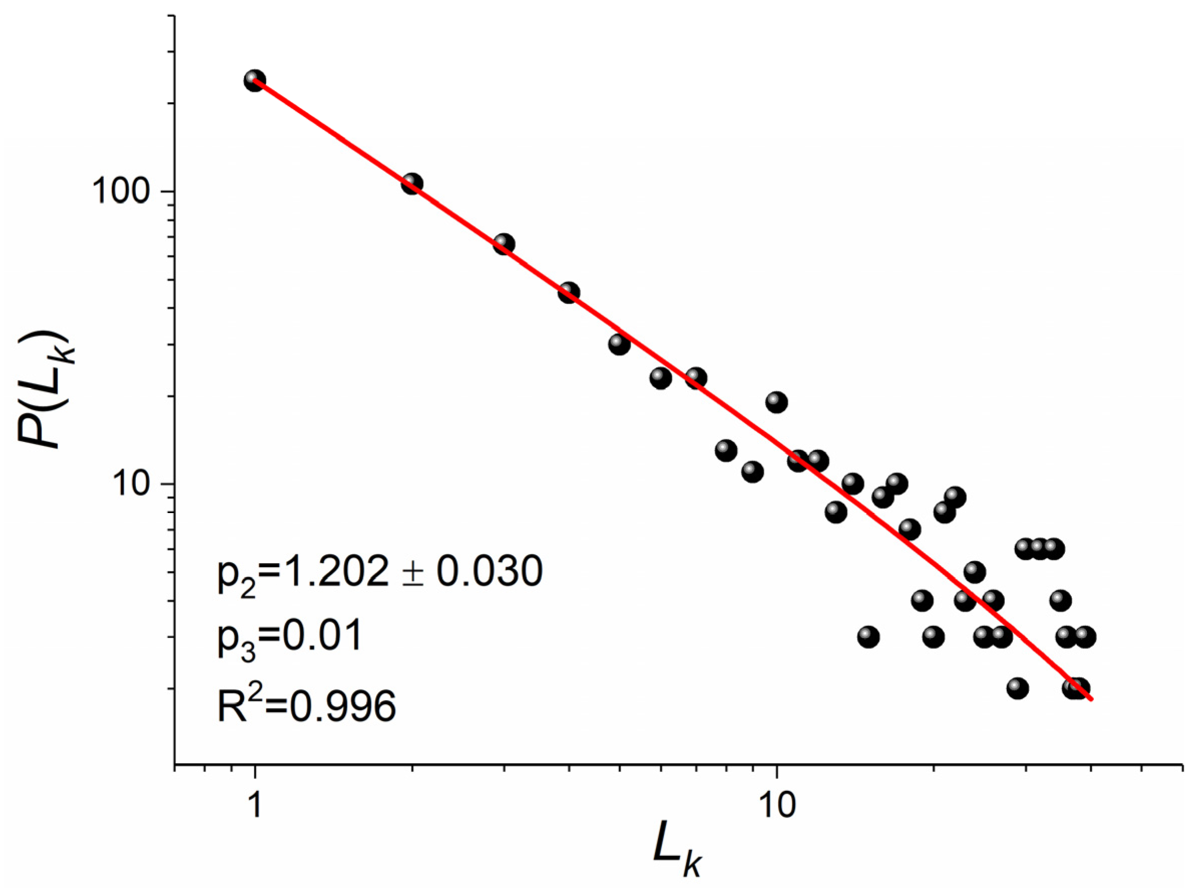
Section 3. It is mentioned that the probabilities of appearance of the two symbols are not the same (46% “+1” vs., 54% “−1”) in the analyzed symbolic time series, thus the specific symbolic time series has statistics closer to the ones of real time series. The result of the PNA-STSM analysis, is that the distribution of the “
waiting lengths” at the central values
of the quantized magnetic field is very close to a power law since
, with power law exponent
(see
Figure 7c). The obtained exponents’ values, i.e.,
and
, indicate that the critical state survives within the hysteresis zone, which is something expected since the studied temperature
is very close to the pseudocritical temperature
.
Analyzing the specific symbolic time series in the time domain, i.e., by analyzing the waiting times at each of the two symbols separately (see
Section 2), one arrives at two different results: for waiting times for the “+1” symbol distribution, the estimated exponents’ values are
, whereas for the waiting times for the symbol “−1” distribution, the estimated values are
. Both sets of exponents’ values indicate that the critical state survives at
, but the estimated power law exponent
is different for each symbol.
Thus, one cannot reach a definite quantitative result by employing the time domain analysis. On the contrary, the use of the PNA-STSM, which considers both symbolic dynamics’ branches simultaneously, leads to a single power law exponent (), providing a definite quantitative result. It should be finally mentioned that the value of the exponent estimated using the PNA-STSM cannot be obtained by any linear combination of the two different power law exponent values estimated using the time domain analysis, e.g., as their mean value. This also indicates the strong nonlinearity and complexity of the examined system.
4.2. The Case of the Nano-MOSFET Electronic Device
The second case studied regards an ultrathin body and buried box (UTBB) fully depleted silicon-on-insulator (FD-SOI) nano-MOSFET. This device was fabricated with channel dimensions W = 0.5 μm and L = 30 nm, while the silicon film thickness was t
Si = 7 nm [
25]. Finally, the box thickness was 25 nm, and the equivalent front gate oxide thickness was (EOT) t
ox = 1.55 nm (TiN/HfSiON stack) [
25]. Fully depleted silicon-on-insulator MOSFETs [
26,
27] exhibit low threshold voltage and threshold voltage controllability (by the second gate bias) at the nanoscale. Because of its compatibility to the standard planar CMOS technology, it is capable of further downscaling; therefore, the characteristics of noise currents are crucial to study. Next to typical noise analysis [
25], UTBB-FD-SOI nano-MOSFET has also been studied from the point of view of nonlinear dynamics [
28], critical phenomena [
29], as well as Tsallis non-extensive statistics [
30]. All three approaches confirmed the deterministic origin of demonstrated random telegraph noise (RTN).
In the following, we present the analysis of the above-mentioned nano-MOSFET’s drain current
time series of a duration of 5 s, sampled at a sampling period of
, thus consisting of 100,000 points. The drain current has been acquired for bias conditions:
,
, and
, while
acted as a control parameter.
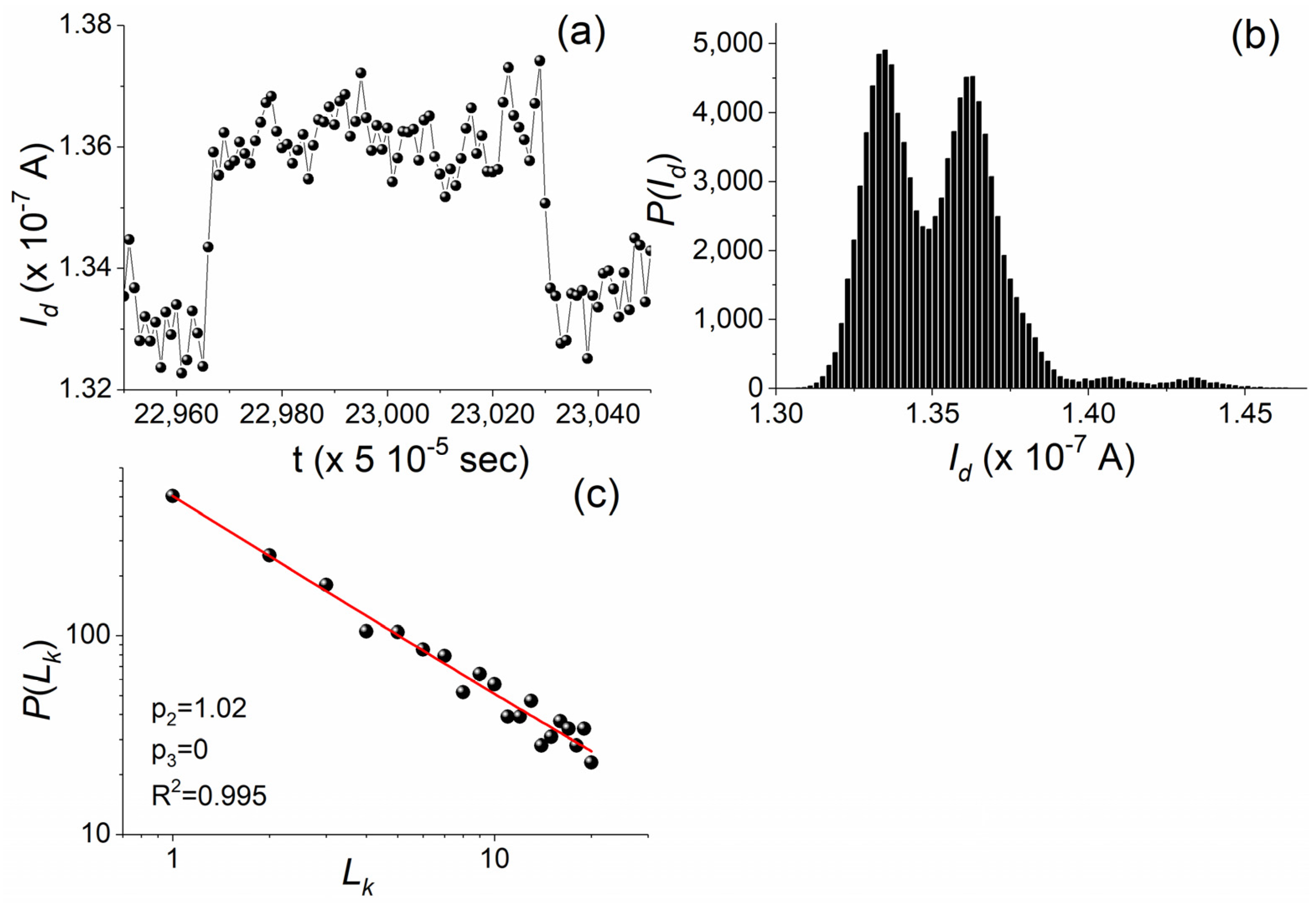
Figure 8a portrays a small segment of the analyzed time series to illustrate that
values fluctuate around two current levels, hereafter referred to as “HIGH values” and “LOW values”, respectively. In the case of the specific nano-MOSFET on–off intermittency occurs between HIGH and LOW values. One can easily identify the bimodal form of the corresponding time series values’ histogram (
Figure 8b), while the two lobes are not completely separated from each other; thus, they “communicate”. If one defines as “separation point” between the two lobes of the distribution of the histogram bin of the smallest statistic (
), a straightforward way to obtain a two-state coarse-graining description of the
value for the specific experiment is to assign time series values
and
to the symbols “+1” (HIGH value) and “−1” (LOW value), respectively.
As soon as the original real-valued time series was converted into a two-symbol symbolic time series, PNA-STSM analysis was applied (see
Section 3.1). The result is presented in
Figure 8c, showing that the distribution of the “
waiting lengths” at the central values
of the quantized magnetic field is an exact power law (
) with power law exponent
. Since the nominal value of the estimated power law exponent is
, we confirm that the dynamics embedded in the
symbolic time series are indeed critical dynamics; but notice that at the lower error limit, the tricritical dynamics appears (
). This entanglement of the critical and the tricritical points is confirmed by the theory of critical phenomena. Indeed, according to the
theory in the parametric space of the Landau free energy, where the coefficients of the
and
terms of the Landau polynomial serve as the parameters, meeting of the lines of the second-order phase transition and the first-order phase transition takes place [
16]. Thus, the critical point, which is the endpoint of the second-order phase transition line, meets the tricritical point, which is the starting point of the first-order phase transition line. Therefore, the result obtained by the PNA-STSM indicates exactly the above-mentioned meeting that the theory predicts.
It is also interesting to see the results obtained if one analyzes the specific symbolic time series in the time domain, i.e., by analyzing the waiting times at each of the two symbols separately (see
Section 2). The time domain analysis of the waiting times for the “+1” symbol distribution leads to the set of exponents
; while for the distribution of the waiting times for the “−1” symbol, one obtains
. In both cases, an exact power law fits the waiting times distribution. However, although the probabilities of the appearance of the two symbols are very close, 49% (“+1”) vs. 51% (“−1”), the two estimated power law exponents differ. Importantly, on the one hand, the nominal value of the power law exponent estimated for the “−1” symbol distribution is
, indicating a critical state; on the other hand, the nominal value of the power law exponent estimated for the “+1” symbol distribution is
, which denotes a tricritical state. Additionally, considering the error limits of the two estimated
values, one finds that the
value resulting from the “−1” branch is clearly in the critical state, contrary to the one resulting from the “+1” branch that is mainly in the tricritical state, but also marginally enters the critical state. Thus, by means of the time domain waiting times analysis, one cannot definitely answer the question of what are the dynamics to which the drain current fluctuations obey. On the contrary, as already shown above, the PNA-STSM analysis, which simultaneously considers the information from both symbols, provides a clear answer.
4.3. The Case of the Presismic MHz Fracto-Electromagnetic Emission
As has been shown in [
31,
32], earthquake (EQ) preparation processes present remarkable analogies to thermal systems, as studied through the analysis of FEME/FEMR in the MHz band. Specifically, the spin organization mechanism of the 3D Ising model presents striking similarities, both in qualitative and quantitative terms, with the pre-seismic organization of a strong EQ. As already mentioned in
Section 4, in finite thermal systems, the transition from the critical state to the SSB occurs gradually as the temperature drops. The characteristic of this temperature transition zone is the communication of the two lobes of the mean magnetization distribution. As soon as this communication stops, the two lobes completely separate, signifying the completion of the SSB. In the FEME/FEMR time series recorded before the EQ occurrence in the MHz band, there can be found segments of the signal values distributions which are bimodal, while the two lobes communicate with one another, as it happens with the mean magnetization of the 3D Ising model within the zone between the critical state and the SSB.
In the following example, we refer to a shallow, very strong EQ (
) which occurred on 14 February 2008 offshore Methoni town (South-West Peloponnese, Greece). Two days before the EQ occurrence, the 41 MHz receiver of the ELSEM-Net (hELlenic Seismo-ElectroMagnetics Network,
http://elsemnet.uniwa.gr, (accessed on 8 June 2023) station located in Zakynthos (Zante) Island recorded the 40,000-sec-long time series excerpt depicted in
Figure 9a (sampling period = 1 s, the receiver output voltage,
, is directly related to the received electric field level at 41 MHz). As shown in
Figure 9b, the specific time series excerpt presents a bimodal amplitude distribution, while the two lobes are again not completely separated.
Although
Figure 9a does not resemble the familiar structure of on–off intermittency encountered in the two previous time series of the examples utilized (
Section 4.1 and
Section 4.2), one could consider that it presents a kind of on–off intermittency with only a single alternation between two value levels (HIGH and LOW), around which fluctuations occur. If one defines as “separation point” between the two lobes of the distribution of
Figure 9b, the histogram bin of the smallest statistic (
), a straightforward way to obtain a two-state coarse-graining description of the
values could be established. For the specific recording, we assigned time series values
and
to the symbols “+1” (HIGH value) and “−1” (LOW value), respectively. It must be noted that the exact position of the “separation point” does not substantially affect the results.
After converting the real-valued time series of the MHz FEME/FEMR recordings into a two-symbol symbolic time series, the PNA-STSM analysis was applied (see
Section 3.1). The result is presented in
Figure 9c, showing that the eight first points of the distribution of the “
waiting lengths” at the central values
of the quantized magnetic field can be fitted by a power law with exponent
, which declares the critical state. In studying MHz FEME/FEMR precursors, it is very important to reveal the information embedded in time series excerpts, such as the presented one, that present bimodal amplitude distributions because such time series segments herald the upcoming complete separation of the two lobes. As already mentioned, the complete separation of the two lobes signifies the completion of the SSB, which leads to preferred directions in the organization of the fractures in the focal area [
31,
32]. In other words, it leads to ruptures that may result in seismic events. In
Figure 9d, we present the values’ distribution of such an SBB time series excerpt that was recorded after the critical segment of
Figure 9a. The specific SSB excerpt was 18,000-sec-long and was completed just 3.5 h before the examined EQ.
We finally mention that if one tries to analyze the same symbolic time series in the time domain, i.e., by analyzing the waiting times at each of the two symbols separately (see
Section 2), a very different, in fact false, picture is drawn. As shown in [
33], a power law distribution of the waiting times with exponent
indicates that the critical organization is achieved by the domination of the Lévy process, which may result in the occurrence of a strong EQ, while if
, then a slow transition from the Lévy to the Gaussian process appears, which means that a strong EQ should not be expected to follow. Our “a posteriori” analysis by means of the PNA-STSM yielded a single power law exponent
, which is a result in perfect agreement with the fact that a strong EQ indeed occurred after the analyzed MHz FEME/FEMR time series excerpt of
Figure 9a. On the contrary, the time domain analysis of the waiting times at the “+1” symbol distribution estimates an exponent
, which leads to the false conclusion that a strong EQ should not be expected to follow, whereas time domain analysis of the waiting times at the “−1” symbol results to a waiting times distribution that does not follow any power law. Therefore, PNA-STSM is the only credible way to retrieve the information embedded in MHz FEME/FEMR precursors time series excerpts that present bimodal amplitude distributions, such as the presented one.


 ,
, 


