Numerical Analysis of Nonlinear Coupled Schrödinger–KdV System with Fractional Derivative

Abstract

In this paper, we propose two efficient methods for solving the fractional-order Schrödinger–KdV system. The first method is the Laplace residual power series method (LRPSM), which involves expressing the solution as a power series and using residual correction to improve the accuracy of the solution. The second method is a new iterative method (NIM) that simplifies the problem and obtains a recursive formula for the solution. Both methods are applied to the Schrödinger–KdV system with fractional derivatives, which arises in many physical applications. Numerical experiments are performed to compare the accuracy and efficiency of the two methods. The results show that both methods can produce highly accurate solutions for the fractional Schrödinger–KdV system. However, the new iterative method is more efficient in terms of computational time and memory usage. Overall, our study demonstrates the effectiveness of the residual power series method and the new iterative method in solving fractional-order Schrödinger–KdV systems and provides a valuable tool for researchers and practitioners in applied mathematics and physics.

1. Introduction

The Schrödinger–KdV system is a nonlinear coupled system of partial differential equations that describes the evolution of a wave packet in a medium that exhibits dispersive and nonlinear effects. The system is widely used to model many physical phenomena, such as plasma physics, fluid dynamics, and quantum mechanics. However, in recent years, there has been a growing interest in the study of fractional differential equations, which involve derivatives of noninteger order [1,2,3]. The fractional-order Schrödinger–KdV system is a generalization of the classical Schrödinger–KdV system, in which fractional derivatives replace the derivatives. The fractional-order derivatives have been found to model many complex physical phenomena, such as anomalous diffusion, viscoelasticity, and wave propagation in fractal media. The fractional-order Schrödinger–KdV system has attracted much attention in the literature due to its rich dynamical behaviors, including soliton solutions, chaos, and wave-packet spreading [4,5].

The study of fractional-order Schrödinger–KdV systems is challenging due to the nonlinearity and complexity of the equations involved. Analytical solutions are rarely available, and numerical methods are often needed to approximate the solutions. This paper proposes two numerical methods, the residual power series method and the new iterative method, to efficiently solve the fractional-order Schrödinger–KdV system [6,7].

Symmetry is a fundamental concept in various scientific disciplines, playing a crucial role in understanding the underlying principles governing natural phenomena and mathematical structures. It provides a powerful framework for simplifying and analyzing complex systems, leading to the discovery of elegant solutions and insights. This notion of symmetry has found applications in various fields, ranging from physics and engineering to mathematics and beyond. The symmetry analysis of mathematical models plays a crucial role in unveiling complex systems’ underlying structure and behavior. One such intriguing system is the Schrödinger–KdV system, which combines elements of quantum mechanics and nonlinear wave propagation. This system’s study enriches our understanding of fundamental physical phenomena and has implications in various interdisciplinary fields. By investigating the symmetries inherent in Schrödinger–KdV, researchers can gain insights into its intrinsic properties and potentially reveal novel analytical solutions. In recent research endeavors, scholars have explored applying symmetry principles to address challenging problems across different domains. Notably, Lyu and Wang [8] delve into reaction–diffusion systems with density-suppressed motility, unraveling global classical solutions through symmetry-based approaches. He, Peng, and Li [9] present an innovative iterative approximation technique for fixed point problems and variational inequality problems on Hadamard manifolds, further extending this approach in He, Peng, and Li [10] to implicit viscosity iterative algorithms. The influence of symmetry extends to diverse fields, encompassing control systems and robotics. Zhang et al. [11] examine L2-gain adaptive robust control for hybrid energy storage systems in electric vehicles, showcasing the integration of symmetry concepts into advanced control strategies. Wang, Zhang, and Zhang [12] propose a composite adaptive fault-tolerant attitude control for a quadrotor UAV, harnessing symmetry principles to enhance the system’s robustness. Symmetry’s significance also resonates in logistics and supply chain management. Li et al. [13] explore H consensus for multi-agent-based supply chain systems under switching topology and uncertain demands, utilizing symmetry principles to optimize coordination and efficiency. Beyond these applications, symmetry-driven methodologies find expression in fields such as marine science [14], renewable energy systems [15], nonlinear system stabilization [16], and advanced control design [17].

The field of applied mathematics, fractional calculus (FC), deals with arbitrary-order derivatives and integrals. Due to their proven uses in research and engineering, fractional differential equations have gained significance and appeal. These equations are gradually used to model a wide range of physical phenomena, including theology, fluid dynamics, oscillation, diffusion, reaction–diffusion, anomalous diffusion, diffusive transport analogous to diffusion, turbulence, polymer physics, electric networks, corrosion electrochemistry, chemical physics, relaxation processes in complex systems, and dynamical processes in self-similar and porous structures [18,19,20,21]. In this and other applications, the nonlocality of fractional differential equations is the main advantage. Contrary to the integer order differential operator, the fractional-order differential operator is a local operator. This implies that a system’s future state depends on all of its previous and current states. One of the reasons why fractional calculus is gaining popularity is that this is more sincere [22,23,24,25,26]. For many years, the nonlinear Schrödinger equation (NLSE) has been the subject of intensive study. This is a result of the fact that it can be used in many situations. Bose–Einstein condensates, nonlinear optics, fluid dynamics, and other phenomena are among the many NLSEs used to describe events in different fields [27,28,29,30,31].

The coupled fractional Schrödinger–KdV equation is given by

$$\begin{array}{cc}\hfill & D_t^{\alpha }\eta (ß,t)-\frac{{\partial }^2\eta (ß,t)}{\partial {ß}^2}-\xi (ß,t)\delta (ß,t)=0,0<\alpha \le 1\hfill \\ \hfill & D_t^{\alpha }\xi (ß,t)-\frac{{\partial }^2\xi (ß,t)}{\partial {ß}^2}+\eta (ß,t)\delta (ß,t)=0,\hfill \\ \hfill & D_t^{\alpha }\delta (ß,t)+\frac{{\partial }^3\delta (ß,t)}{\partial {ß}^3}+6\delta (ß,t)\frac{\partial \delta (ß,t)}{\partial ß}-2\eta (ß,t)\frac{\partial \delta (ß,t)}{\partial ß}-2\xi (ß,t)\frac{\partial \xi (ß,t)}{\partial ß}=0.\hfill \end{array}$$

(1)

The Laplace residual power series method (LRPSM) is used to find an approximate solution to the given equations. LRPSM [32,33,34,35,36] is a mixture of the residual power series method (RPSM) and Laplace transformation (LT) [37,38,39,40,41]. LRPSM, the technique applied, is fast, simple, and adaptable to solving fractional partial differential equations and others. For many years, the nonlinear Schrödinger equation (NLSE) has been the subject of intensive study. This is a result of the fact that it can be used in many situations. Bose–Einstein condensates, nonlinear optics, fluid dynamics, and other phenomena are some of the numerous NLSEs used to analyze events in different fields.

This paper presents two efficient methods for solving the fractional-order Schrödinger–KdV system, a complex mathematical model relevant in various physical contexts. The proposed Laplace residual power series method (LRPSM) expresses the solution as a power series, utilizing residual correction to enhance accuracy, while the new iterative method (NIM) employs the Laplace transform to simplify the problem and derive a recursive solution formula. Both methods are applied to the fractional Schrödinger–KdV system and are validated through numerical experiments, demonstrating their high accuracy. Importantly, NIM is more computationally efficient regarding time and memory usage than LRPSM. The study’s contributions provide valuable tools for researchers and practitioners in applied mathematics and physics, addressing complex fractional-order systems effectively [42,43,44].

An outline of this paper is as follows: In Section 2, we start by providing some preliminaries that are used in our study. The general procedure of the proposed methods LRPSM and NIM for solving the fractional-order Schrödinger–KdV system is provided in Section 3. The implementation of the proposed methods and the discussion of the results are presented in Section 4. Finally, Section 5 includes the conclusions of our study.

2. Preliminaries

Definition 1.

In the sense of Caputo, the fractional derivative of a function $\eta (ß,t)$ of order α is described as [45]

$${}^C{D}_t^{\alpha }\eta (ß,t)=J_t^{m-\alpha }{\eta }^m(ß,t),m-1<\alpha \le m,t>0,$$

(2)

where $m\in N$ and $J_t^{\alpha }$ represent the fractional integral (FI) of $\eta (ß,t)$ by Riemann–Liouville (RL). The definition of fractional order α is

$$J_t^{\alpha }\eta (ß,t)=\frac{1}{\Gamma \left(\alpha \right)}{\int }_0^t{(t-r)}^{\alpha -1}\eta (ß,r)dr,$$

(3)

taking for granted that the provided integral exists.

Definition 2.

A function’s Laplace transformation $\eta (ß,t)$ is given as [46]

$$\eta (ß,s)={\mathcal{L}}_t\left[\eta (ß,t)\right]={\int }_0^{\infty }{e}^{-st}\eta (ß,t)dt,s>\alpha ,$$

(4)

where the inverse Laplace transformation is defined as

$$\eta (ß,t)={\mathcal{L}}_{\tau }^{-1}\left[\eta (ß,s)\right]={\int }_{l-i\infty }^{l+i\infty }{e}^{st}\eta (ß,s)ds,l=Re\left(s\right)>l_0,$$

(5)

where $l_0$ is the absolute convergence of the Laplace integral in the right half-plane.

Lemma 1.

Suppose that $\eta (ß,t)$ is a piecewise continuous term of exponential order ζ and $\eta (ß,s)={\mathcal{L}}_t\left[\eta (ß,t)\right]$, we obtain

1. 

${\mathcal{L}}_t\left[J_t^{\alpha }\eta (ß,t)\right]=\frac{\eta (ß,s)}{s^{\alpha }},\alpha >0.$

2. 

${\mathcal{L}}_t\left[D_t^{\alpha }\eta (ß,t)\right]=s^{\alpha }\eta (ß,s)-{\sum }_{k=0}^{m-1}{s}^{\alpha -k-1}{\eta }^k(ß,0),m-1<\alpha \le m.$

3. 

${\mathcal{L}}_t\left[D_t^{n\alpha }\eta (\eta ,t)\right]=s^{n\alpha }\eta (ß,s)-{\sum }_{k=0}^{n-1}{s}^{(n-k)\alpha -1}{D}_t^{k\alpha }\eta (ß,0),0<\alpha \le 1.$

Remark 1.

The inverse Laplace transformation is shown as [47]

$$\eta (ß,t)=\sum _{i=0}^{\infty }\frac{D_t^{\alpha }\eta (ß,0)}{\Gamma (1+i\alpha )}{t}^{i\left(\zeta \right)},0<\zeta \le 1,t\ge 0.$$

(6)

This corresponds to the fractional Taylor’s formula presented in [48].

3. General Procedure of the Proposed Methods

3.1. LRPSM Procedure

Consider the fractional-order partial differential equation

$$\begin{array}{cc}\hfill & D_t^{\alpha }\eta (ß,t)+N\left[\eta (ß,t)\right]+R\left[\eta (ß,t)\right]=0,\mathrm{where}0<\alpha \le 1,\hfill \end{array}$$

(7)

where $R\left[\eta \right(ß,t\left)\right]$ and $N\left[\eta \right(ß,t\left)\right]$ are linear and nonlinear functions, respectively, with the initial conditions

$$\begin{array}{c}\hfill \eta (ß,0)=f_0(ß).\end{array}$$

(8)

Applying the Laplace transform to Equation (7) and making use of Equation (8), we obtain

$$\begin{array}{c}\hfill \eta (ß,s)-\frac{f_0(ß,s)}{s}+\frac{1}{s^{\alpha }}{\mathcal{L}}_t\left[N\left[{\mathcal{L}}_t^{-1}\left[\eta (ß,s)\right]\right]\right]+\frac{1}{s^{\alpha }}A\left[\eta (ß,s)\right]=0.\end{array}$$

(9)

Suppose that the result of Equation (9) is defined as

$$\begin{array}{cc}\hfill & \eta (ß,s)=\sum _{n=0}^{\infty }\frac{f_n(ß,s)}{s^{n\alpha +1}},\hfill \end{array}$$

(10)

the $k^{th}$-truncated term series are

$$\begin{array}{cc}\hfill & \eta (ß,s)=\frac{f_0(ß,s)}{s}+\sum _{n=1}^k\frac{f_n(ß,s)}{s^{n\alpha +1}},n=1,2,3,4\cdots .\hfill \end{array}$$

(11)

The Laplace residual functions (LRFs) are

$$\begin{array}{c}\hfill {\mathcal{L}}_{t}Res(ß,s)=\eta (ß,s)-\frac{f_0(ß,s)}{s}+\frac{1}{s^{\alpha }}{\mathcal{L}}_t\left[N\left[{\mathcal{L}}_t^{-1}\left[\eta (ß,s)\right]\right]\right]+\frac{1}{s^{\alpha }}A\left[\eta (ß,s)\right].\end{array}$$

(12)

The $k^{th}$-LRFs are

$$\begin{array}{c}\hfill {\mathcal{L}}_{t}Re{s}_k(ß,s)={\eta }_k(ß,s)-\frac{f_0(ß,s)}{s}+\frac{1}{s^{\alpha }}{\mathcal{L}}_t\left[N\left[{\mathcal{L}}_t^{-1}\left[{\eta }_k(ß,s)\right]\right]\right]+\frac{1}{s^{\alpha }}A\left[{\eta }_k(ß,s)\right].\end{array}$$

(13)

To illustrate a few facts, the following LRPSM features are provided:

• ${\mathcal{L}}_{t}Res(ß,s)=0$ and ${\lim }_{j\to \infty }{\mathcal{L}}_{t}Re{s}_k(\eta ,s)={\mathcal{L}}_{t}Re{s}_{\eta }(ß,s)$ for each $s>0.$
• ${\lim }_{s\to \infty }s{\mathcal{L}}_{t}Re{s}_{\eta }(ß,s)=0\Rightarrow {\lim }_{s\to \infty }s{\mathcal{L}}_{t}Re{s}_{\eta ,k}(ß,s)=0.$
• ${\lim }_{s\to \infty }{s}^{k\alpha +1}{\mathcal{L}}_{t}Re{s}_{\eta ,k}(ß,s)={\lim }_{s\to \infty }{s}^{k\alpha +1}{\mathcal{L}}_{t}Re{s}_{\eta ,k}(ß,s)=0,1<\alpha \le 2,k=1,2,3,\cdots$.

To calculate the coefficients using $f_n(ß,s)$, the following system is recursively solved:

$$\begin{array}{cc}\hfill & \underset{s\to \infty }{\lim }{s}^{k\alpha +1}{\mathcal{L}}_{\tau }Re{s}_{\eta ,k}(ß,s)=0,k=1,2,\cdots .\hfill \end{array}$$

(14)

Finally, we apply the inverse Laplace transform to Equation (10) to obtain the $k^{th}$ analytical result of ${\eta }_k(ß,t)$.

3.2. NIM Procedure

Consider the general fractional partial differential equation

$$\begin{array}{c}\hfill \eta (ß)=f(ß)+N\left(\eta \right(ß\left)\right),\end{array}$$

(15)

where f is an unknown function and N is a nonlinear operator. We have been looking for a way to have the series form (15)

$$\begin{array}{cc}\hfill & \eta (ß)=\sum _{i=0}^{\infty }{\eta }_i(ß).\hfill \end{array}$$

(16)

The nonlinear term can be decomposed as

$$\begin{array}{cc}\hfill & N(\sum _{i=0}^{\infty }{\eta }_i(ß)=N\left({\eta }_0\right)+\sum _{i=0}^{\infty }\left[N\left(\sum _{j=0}^i{\eta }_j(ß)\right)-N\left(\sum _{j=0}^{i-1}{\eta }_j(ß)\right)\right].\hfill \end{array}$$

(17)

Equation (16) and Equations (15) and (17) are equivalent to

$$\begin{array}{c}\hfill \sum _{i=0}^{\infty }{\eta }_i(ß)=f+N\left({\eta }_0\right)+\sum _{i=0}^{\infty }\left[N\left(\sum _{j=0}^i{\eta }_j(ß)\right)-N\left(\sum _{j=0}^{i-1}{\eta }_j(ß)\right)\right].\end{array}$$

(18)

The following recurrence relation is defined:

$$\begin{array}{cc}\hfill & {\eta }_0=f,\hfill \\ \hfill & {\eta }_1=N\left({\eta }_0\right),\hfill \\ \hfill & {\eta }_2=N({\eta }_0+{\eta }_1)-N\left({\eta }_0\right),\hfill \\ \hfill & {\eta }_{n+1}=N({\eta }_0+{\eta }_1+\cdots {\eta }_n)-N({\eta }_0+{\eta }_1+\cdots {\eta }_{n-1}),n=1,2,3\cdots .\hfill \end{array}$$

(19)

Then

$$\begin{array}{cc}\hfill & ({\eta }_0+{\eta }_1+\cdots {\eta }_n)=N({\eta }_0+{\eta }_1+\cdots {\eta }_n),n=1,2,3\cdots ,\hfill \\ \hfill & \omega =\sum _{i=0}^{\infty }{\eta }_i(ß)=f+N\left(\sum _{i=0}^{\infty }{\eta }_i(ß)\right).\hfill \end{array}$$

(20)

4. Numerical Problem

In this section, we present the proposed methods on the nonlinear coupled system of fractional-order partial differential equations.

Example 1.

Consider the following time-fractional KdV equation [49]:

$$\begin{array}{c}\hfill D_t^{\alpha }\eta (ß,t)+6\eta (ß,t)\frac{{\partial }^{}\eta (ß,t)}{\partial {ß}^{}}+\frac{{\partial }^3\eta (ß,t)}{\partial {ß}^3}=0,\mathit{where}0<\alpha \le 1,\end{array}$$

(21)

subjected to the following ICs:

$$\begin{array}{c}\hfill \eta (ß,0)=\frac{1}{2}{\mathit{sech}}^2\left(\frac{\beta }{2}\right).\end{array}$$

(22)

Implementation of LRPSM

Applying LT to Equation (21) and making use of Equation (22), we obtain

$$\begin{array}{cc}\hfill & \eta (ß,s)-\frac{\frac{1}{2}{\mathit{sech}}^2\left(\frac{ß}{2}\right)}{s}+\frac{1}{s^{\alpha }}\frac{{\partial }^3\eta (ß,s)}{\partial {ß}^3}+\frac{1}{s^{\alpha }}{\mathcal{L}}_t\left[{\mathcal{L}}_t^{-1}\left[\eta (ß,s)\right]{\mathcal{L}}_t^{-1}\left\{\frac{{\partial }^{}\eta (ß,s)}{\partial {ß}^{}}\right\}\right]=0,\hfill \end{array}$$

(23)

and so the $k^{th}$-truncated term series are

$$\begin{array}{c}\hfill \eta (ß,s)=\frac{\frac{1}{2}{\mathit{sech}}^2\left(\frac{ß}{2}\right)}{s}+\sum _{r=1}^k\frac{f_r(ß,s)}{s^{rp+1}},r=1,2,3,4\cdots .\end{array}$$

(24)

Laplace residual functions (LRFs) are

$$\begin{array}{cc}\hfill & {\mathcal{L}}_{t}Res(ß,s)=\eta (ß,s)-\frac{\frac{1}{2}{\mathit{sech}}^2\left(\frac{ß}{2}\right)}{s}+\frac{1}{s^{\alpha }}\frac{{\partial }^3\eta (ß,s)}{\partial {ß}^3}+\frac{1}{s^{\alpha }}{\mathcal{L}}_t\left[{\mathcal{L}}_t^{-1}\left[\eta (ß,s)\right]{\mathcal{L}}_t^{-1}\left\{\frac{{\partial }^{}\eta (ß,s)}{\partial {ß}^{}}\right\}\right],\hfill \end{array}$$

(25)

and the $k^{th}$-LRFs are

$$\begin{array}{cc}\hfill & {\mathcal{L}}_{t}Re{s}_k(ß,s)={\eta }_k(ß,s)-\frac{\frac{1}{2}{\mathit{sech}}^2\left(\frac{ß}{2}\right)}{s}+\frac{1}{s^{\alpha }}\frac{{\partial }^3{\eta }_k(ß,s)}{\partial {ß}^3}+\frac{1}{s^{\alpha }}{\mathcal{L}}_t\left[{\mathcal{L}}_t^{-1}\left[{\eta }_k(ß,s)\right]{\mathcal{L}}_t^{-1}\left\{\frac{{\partial }^{}{\eta }_k(ß,s)}{\partial {ß}^{}}\right\}\right].\hfill \end{array}$$

(26)

Now, to determine $f_r(ß,s)$, $r=1,2,3,\cdots ,$ we substitute the $r^{th}$-truncated series Equation (24) into the $r^{th}$-Laplace residual function Equation (26), multiply the resulting equation by $s^{r\alpha +1}$, and then solve recursively the relation ${\lim }_{s\to \infty }\left(s^{r\alpha +1}{\mathcal{L}}_{t}Re{s}_{\eta ,r}(ß,s)\right)=0$, $r=1,2,3,\cdots$. The following are the first few terms:

$$\begin{array}{cc}\hfill & f_1(ß,s)=4{\sinh }^4\left(\frac{ß}{2}\right){\mathit{csch}}^3(ß),\hfill \\ \hfill & f_2(ß,s)=\frac{1}{4}(\cosh (ß)-2){\mathit{sech}}^4\left(\frac{ß}{2}\right),\hfill \end{array}$$

(27)

and so on

$$\begin{array}{cc}\hfill & \eta (ß,s)=\frac{\frac{1}{2}{\mathit{sech}}^2\left(\frac{ß}{2}\right)}{s}+\frac{4{\sinh }^4\left(\frac{ß}{2}\right){\mathit{csch}}^3(ß)}{s^{\alpha +1}}+\frac{\frac{1}{4}(\cosh (ß)-2){\mathit{sech}}^4\left(\frac{ß}{2}\right)}{s^{\alpha }}+\cdots .\hfill \end{array}$$

(28)

Using the inverse Laplace transform,

$$\begin{array}{cc}\hfill & \eta (ß,s)=\frac{1}{2}{\mathit{sech}}^2\left(\frac{ß}{2}\right)+\frac{4{\sinh }^4\left(\frac{ß}{2}\right){\mathit{csch}}^3(ß)}{\Gamma \left(\alpha +1\right)}{t}^{\alpha }+\frac{\frac{1}{4}(\cosh (ß)-2){\mathit{sech}}^4\left(\frac{ß}{2}\right)}{\Gamma \left(2\alpha +1\right)}{t}^{2\alpha }+\cdots .\hfill \end{array}$$

(29)

Implementation of NIM

Applying the RL integral to Equation (21), we obtain the equivalent form

$$\begin{array}{c}\hfill \eta (ß,t)=\frac{1}{2}{\mathit{sech}}^2\left(\frac{ß}{2}\right)-I_t^{\alpha }\left[6\eta (ß,t)\frac{{\partial }^{}\eta (ß,t)}{\partial {ß}^{}}+\frac{{\partial }^3\eta (ß,t)}{\partial {ß}^3}\right]\end{array}$$

(30)

According to the NIM procedure, we obtain the following few terms:

$$\begin{array}{cc}\hfill & {\eta }_0(ß,t)=\frac{1}{2}{\mathit{sech}}^2\left(\frac{ß}{2}\right),\hfill \\ \hfill & {\eta }_1(ß,t)=\frac{4{\sinh }^4\left(\frac{ß}{2}\right){\mathit{csch}}^3(ß)t^p}{p\Gamma \left(p\right)},\hfill \\ \hfill & {\eta }_2(ß,t)=\frac{1}{4}(\cosh (ß)-2){\mathit{sech}}^4\left(\frac{ß}{2}\right)t^{2\alpha }\left(\frac{1}{\Gamma (2\alpha +1)}+\frac{4^{\alpha }\tanh \left(\frac{ß}{2}\right){\mathit{sech}}^2\left(\frac{ß}{2}\right)t^{\alpha }\Gamma \left(\alpha +\frac{1}{2}\right)}{\sqrt{\pi }{\alpha }^2\Gamma \left(\alpha \right)\Gamma \left(3\alpha \right)}\right).\hfill \end{array}$$

(31)

Using the NIM formulation, we obtain the approximation

$$\begin{array}{cc}\hfill & \eta (ß,t)=\frac{1}{2}{\mathit{sech}}^2\left(\frac{ß}{2}\right)+\frac{4{\sinh }^4\left(\frac{ß}{2}\right){\mathit{csch}}^3(ß)t^p}{p\Gamma \left(p\right)}+\frac{1}{4}(\cosh (ß)-2){\mathit{sech}}^4\left(\frac{ß}{2}\right)t^{2\alpha }\left(\frac{1}{\Gamma (2\alpha +1)}+\right.\hfill \\ & \left.\frac{4^{\alpha }\tanh \left(\frac{ß}{2}\right){\mathit{sech}}^2\left(\frac{ß}{2}\right)t^{\alpha }\Gamma \left(\alpha +\frac{1}{2}\right)}{\sqrt{\pi }{\alpha }^2\Gamma \left(\alpha \right)\Gamma \left(3\alpha \right)}\right)+\cdots \hfill \end{array}$$

(32)

The exact solution for $\alpha =1$ is

$$\begin{array}{cc}\hfill & \eta (ß,t)=\frac{1}{2}{\mathit{sech}}^2\left(\frac{ß-t}{2}\right)\hfill \end{array}$$

(33)

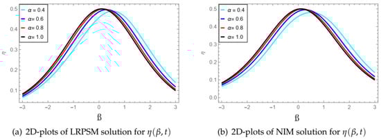
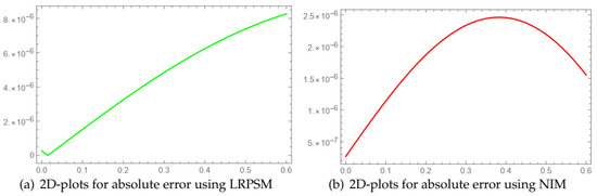
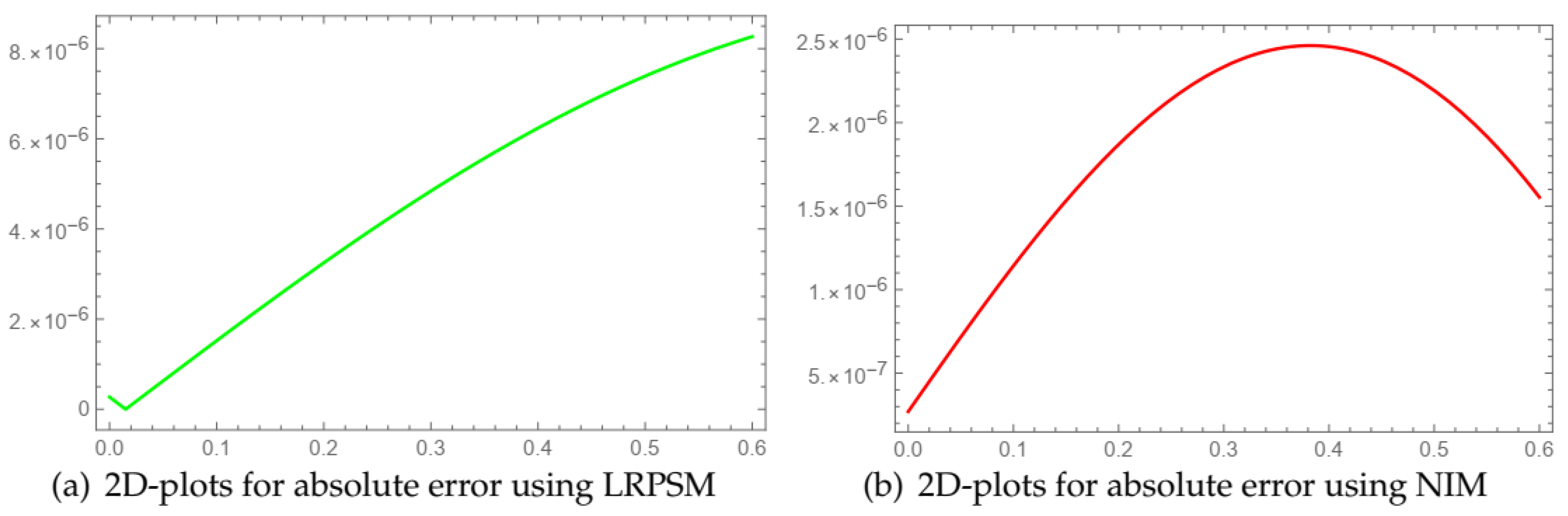
In Figure 1a, the LRPSM solution for $\eta (ß,t)$ is depicted in a 2D plot, offering insight into the system’s behavior. Similarly, Figure 1b portrays the 2D plot of the NIM solution for $\eta (ß,t)$, providing a comparative visual analysis of the two methods for Example 1. The variations observed in these plots contribute to understanding the influence of each method on the solution. Figure 2a displays 2D plots illustrating the absolute error analysis using LRPSM for Example 1. This graphical representation of the absolute error distribution offers a comprehensive view of the accuracy achieved by the LRPSM method. In Figure 1b, the corresponding 2D plots of absolute error using NIM are presented, allowing for a direct comparison of the error profiles produced by the two methods.

Table 1. Numerical values of $\eta (ß,t)$ by using NIM and LRPSM and their absolute error at $\alpha =1$.

ß	$\mathit{\eta }{\mathbf{(}\mathbf{ß}\mathbf{,}\mathit{t}\mathbf{)}}_{\mathit{NIM}}$	$\mathit{\eta }{\mathbf{(}ß\mathbf{,}\mathit{t}\mathbf{)}}_{\mathit{LRPSM}}$	$\mathit{Abs}\mathbf{.}\mathit{error}\mathbf{\left(}\mathit{NIM}\mathbf{\right)}$	$\mathit{Abs}\mathbf{.}\mathit{error}\mathbf{\left(}\mathit{LRPSM}\mathbf{\right)}$
0.1	0.49885	0.49885	5.24347 $\times {10}^{-10}$	2.65047 $\times {10}^{-10}$
0.2	0.495229	0.495229	1.03199 $\times {10}^{-9}$	4.84593 $\times {10}^{-10}$
0.3	0.489206	0.489206	1.4969 $\times {10}^{-9}$	6.29355 $\times {10}^{-10}$
0.4	0.480899	0.480899	1.90139 $\times {10}^{-9}$	6.74469 $\times {10}^{-10}$
0.5	0.470466	0.470466	2.23189 $\times {10}^{-9}$	6.07651 $\times {10}^{-10}$
0.6	0.4581 00	0.458100	2.47961 $\times {10}^{-9}$	4.30081 $\times {10}^{-10}$
0.7	0.444021	0.444021	0.64079 $\times {10}^{-9}$	1.55325 $\times {10}^{-10}$
0.8	0.428469	0.428469	2.71647 $\times {10}^{-9}$	1.93312 $\times {10}^{-10}$
0.9	0.411693	0.411693	2.71195 $\times {10}^{-9}$	5.86445 $\times {10}^{-10}$
1	0.39395	0.39395	2.6359 $\times {10}^{-9}$	9.92581 $\times {10}^{-10}$

provides a tabulated summary of the numerical values of $\eta (ß,t)$ obtained using both NIM and LRPSM methods for Example 1. The table includes the computed values and highlights the absolute error at $\alpha =1$, providing quantitative insight into the accuracy and performance of each method for this specific fractional order.

Table 2. Numerical values of $\eta (ß,t)$ by using NIM and LRPSM with dissimilar values of fractional order $\alpha =0.4$, $\alpha =0.6$, and $\alpha =0.8$.

ß	${\mathit{NIM}}_{\mathit{\alpha }=0.4}$	${\mathit{LRPSM}}_{\mathit{\alpha }=0.4}$	${\mathit{NIM}}_{\mathit{\alpha }=0.6}$	${\mathit{LRPSM}}_{\mathit{\alpha }=0.6}$	${\mathit{NIM}}_{\mathit{\alpha }=0.8}$	${\mathit{LRPSM}}_{\mathit{\alpha }=0.8}$
0.1	0.434414	0.440173	0.475125	0.476806	0.492521	0.492951
0.2	0.442031	0.453097	0.481234	0.484463	0.496035	0.49686
0.3	0.448889	0.464403	0.485383	0.489911	0.497171	0.498328
0.4	0.455015	0.473809	0.487534	0.493019	0.495917	0.49732
0.5	0.460346	0.481064	0.487657	0.493704	0.492302	0.493848
0.6	0.46473	0.48596	0.485733	0.49193	0.486393	0.487977
0.7	0.467943	0.488344	0.48176	0.487715	0.478294	0.479817
0.8	0.469719	0.488128	0.475755	0.481128	0.468146	0.46952
0.9	0.469782	0.48529	0.467762	0.472288	0.456117	0.457274
1	0.467887	0.479877	0.457859	0.461359	0.442404	0.443299

presents a comprehensive comparison of numerical results for $\eta (ß,t)$ obtained using NIM and LRPSM methods, considering different fractional orders, $\alpha =0.4$, $\alpha =0.6$, and $\alpha =0.8$, for Example 1. This table enables a detailed assessment of the impact of varying fractional orders on the solutions obtained by each method, facilitating a deeper understanding of their respective behaviors.

Example 2.

Consider the following time-fractional KdV equation:

$$\begin{array}{c}\hfill D_t^{\alpha }\eta (ß,t)-6\eta (ß,t)\frac{{\partial }^{}\eta (ß,t)}{\partial {ß}^{}}+\frac{{\partial }^3\eta (ß,t)}{\partial {ß}^3}=0,\mathit{where}0<\alpha \le 1,\end{array}$$

(34)

subjected to the following ICs:

$$\begin{array}{c}\hfill \eta (ß,0)=\frac{ß-2}{12}.\end{array}$$

(35)

Implementation of LRPSM

Applying LT to Equation (34) and making use of Equation (35), we obtain

$$\begin{array}{cc}\hfill & \eta (ß,s)-\frac{\frac{ß-2}{12}}{s}+\frac{1}{s^{\alpha }}\frac{{\partial }^3\eta (ß,s)}{\partial {ß}^3}-6\frac{1}{s^{\alpha }}{\mathcal{L}}_t\left[{\mathcal{L}}_t^{-1}\left[\eta (ß,s)\right]{\mathcal{L}}_t^{-1}\left\{\frac{{\partial }^{}\eta (ß,s)}{\partial {ß}^{}}\right\}\right]=0,\hfill \end{array}$$

(36)

and so the $k^{th}$-truncated term series are

$$\begin{array}{c}\hfill \eta (ß,s)=\frac{\frac{ß-2}{12}}{s}+\sum _{r=1}^k\frac{f_r(ß,s)}{s^{rp+1}},r=1,2,3,4\cdots .\end{array}$$

(37)

Laplace residual functions (LRFs) are

$$\begin{array}{cc}\hfill & {\mathcal{L}}_{t}Res(ß,s)=\eta (ß,s)-\frac{\frac{ß-2}{12}}{s}+\frac{1}{s^{\alpha }}\frac{{\partial }^3\eta (ß,s)}{\partial {ß}^3}-6\frac{1}{s^{\alpha }}{\mathcal{L}}_t\left[{\mathcal{L}}_t^{-1}\left[\eta (ß,s)\right]{\mathcal{L}}_t^{-1}\left\{\frac{{\partial }^{}\eta (ß,s)}{\partial {ß}^{}}\right\}\right],\hfill \end{array}$$

(38)

and the $k^{th}$-LRFs are

$$\begin{array}{cc}\hfill & {\mathcal{L}}_{t}Re{s}_k(ß,s)={\eta }_k(ß,s)-\frac{\frac{ß-2}{12}}{s}+\frac{1}{s^{\alpha }}\frac{{\partial }^3{\eta }_k(ß,s)}{\partial {ß}^3}-6\frac{1}{s^{\alpha }}{\mathcal{L}}_t\left[{\mathcal{L}}_t^{-1}\left[{\eta }_k(ß,s)\right]{\mathcal{L}}_t^{-1}\left\{\frac{{\partial }^{}{\eta }_k(ß,s)}{\partial {ß}^{}}\right\}\right],\hfill \end{array}$$

(39)

Now, to determine $f_r(ß,s)$, $r=1,2,3,\cdots ,$ we substitute the $r^{th}$-truncated series Equation (37) into the $r^{th}$-Laplace residual function Equation (39), multiply the resulting equation by $s^{r\alpha +1}$, and then solve recursively the relation ${\lim }_{s\to \infty }\left(s^{r\alpha +1}{\mathcal{L}}_{t}Re{s}_{\eta ,r}(ß,s)\right)=0$, $r=1,2,3,\cdots$. The following are the first few terms:

$$\begin{array}{cc}\hfill & f_1(ß,s)=\frac{ß-2}{24},\hfill \\ \hfill & f_2(ß,s)=\frac{1}{12}-\frac{ß}{24},\hfill \end{array}$$

(40)

and so on

$$\begin{array}{cc}\hfill & \eta (ß,s)=\frac{\frac{ß-2}{12}}{s}+\frac{\frac{ß-2}{24}}{s^{\alpha +1}}+\frac{\frac{1}{12}-\frac{ß}{24}}{s^{\alpha }}+\cdots .\hfill \end{array}$$

(41)

Using the inverse Laplace transform,

$$\begin{array}{cc}\hfill & \eta (ß,s)=\frac{ß-2}{12}+\frac{\frac{ß-2}{24}}{\Gamma \left(\alpha +1\right)}{t}^{\alpha }+\frac{\frac{1}{12}-\frac{ß}{24}}{\Gamma \left(2\alpha +1\right)}{t}^{2\alpha }+\cdots .\hfill \end{array}$$

(42)

Implementation of NIM

Applying the RL integral to Equation (34), we obtain the equivalent form

$$\begin{array}{c}\hfill \eta (ß,t)=\frac{ß-2}{12}-I_t^{\alpha }\left[-6\eta (ß,t)\frac{{\partial }^{}\eta (ß,t)}{\partial {ß}^{}}+\frac{{\partial }^3\eta (ß,t)}{\partial {ß}^3}\right]\end{array}$$

(43)

According to the NIM procedure, we obtain the following few terms:

$$\begin{array}{cc}\hfill & {\eta }_0(ß,t)=\frac{ß-2}{12},\hfill \\ \hfill & {\eta }_1(ß,t)=\frac{(ß-2)t^{\alpha }}{24\alpha \Gamma \left(\alpha \right)},\hfill \\ \hfill & {\eta }_2(ß,t)=\frac{1}{288}(ß-2)t^{2\alpha }\left(\frac{12}{\Gamma (2\alpha +1)}+\frac{4^{\alpha }\Gamma \left(\alpha +\frac{1}{2}\right)t^{\alpha }}{\sqrt{\pi }{\alpha }^2\Gamma \left(\alpha \right)\Gamma \left(3\alpha \right)}\right).\hfill \end{array}$$

(44)

Using the NIM formulation, we obtain the approximation

$$\begin{array}{cc}\hfill & \eta (ß,t)=\frac{ß-2}{12}+\frac{(ß-2)t^{\alpha }}{24\alpha \Gamma \left(\alpha \right)}+\frac{1}{288}(ß-2)t^{2\alpha }\left(\frac{12}{\Gamma (2\alpha +1)}+\frac{4^{\alpha }\Gamma \left(\alpha +\frac{1}{2}\right)t^{\alpha }}{\sqrt{\pi }{\alpha }^2\Gamma \left(\alpha \right)\Gamma \left(3\alpha \right)}\right)+\cdots .\hfill \end{array}$$

(45)

The exact solution for $\alpha =1$ is

$$\begin{array}{cc}\hfill & \eta (ß,t)=\frac{ß-2}{12-6t}.\hfill \end{array}$$

(46)

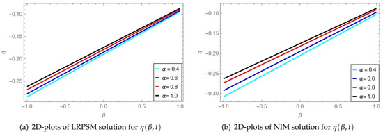
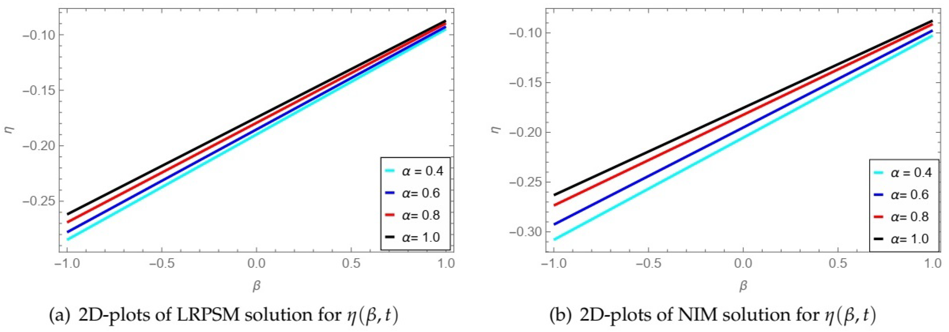
In Figure 3a, the LRPSM solution for $\eta (ß,t)$ is depicted in a 2D plot, offering insight into the system’s behavior. Similarly, Figure 1b portrays the 2D plot of the NIM solution for $\eta (ß,t)$, providing a comparative visual analysis of the two methods for Example 1. The variations observed in these plots contribute to understanding the influence of each method on the solution.

Example 3.

Consider the fractional Schrödinger–KdV equation [50]:

$$\begin{array}{cc}\hfill & D_t^{\alpha }\eta (ß,t)-\frac{{\partial }^2\eta (ß,t)}{\partial {ß}^2}-\xi (ß,t)\delta (ß,t)=0,0<\alpha \le 1,\hfill \\ \hfill & D_t^{\alpha }\xi (ß,t)-\frac{{\partial }^2\xi (ß,t)}{\partial {ß}^2}+\eta (ß,t)\delta (ß,t)=0,\hfill \\ \hfill & D_t^{\alpha }\delta (ß,t)+\frac{{\partial }^3\delta (ß,t)}{\partial {ß}^3}+6\delta (ß,t)\frac{\partial \delta (ß,t)}{\partial ß}-2\eta (ß,t)\frac{\partial \delta (ß,t)}{\partial ß}-2\xi (ß,t)\frac{\partial \xi (ß,t)}{\partial ß}=0,\hfill \end{array}$$

(47)

along with the initial conditions:

$$\begin{array}{cc}\hfill & \eta (ß,0)=\cos (ß),\hfill \\ \hfill & \xi (ß,0)=\sin (ß),\hfill \\ \hfill & \delta (ß,0)=\frac{3}{4}.\hfill \end{array}$$

(48)

Implementation of the Laplace Residual Power Series Method (LRPSM)

Applying LT to Equation (47) and making use of Equation (48), we obtain

$$\begin{array}{cc}\hfill & \eta (ß,s)-\frac{\cos (ß)}{s}-\frac{1}{s^{\alpha }}\left[\frac{{\partial }^2\eta (ß,s)}{\partial {ß}^2}\right]-\frac{1}{s^{\alpha }}\mathcal{L}\left[{\mathcal{L}}_t^{-1}\left[\xi (ß,s)\right]{\mathcal{L}}_t^{-1}\left[\delta (ß,s)\right]\right]=0,\hfill \\ \hfill & \xi (ß,s)-\frac{\sin (ß)}{s}-\frac{1}{s^{\alpha }}\left[\frac{{\partial }^2\xi (ß,s)}{\partial {ß}^2}\right]+\frac{1}{s^{\alpha }}\mathcal{L}\left[{\mathcal{L}}_t^{-1}\left[\eta (ß,s)\right]{\mathcal{L}}_t^{-1}\left[\delta (ß,s)\right]\right]=0,\hfill \\ \hfill & \delta (ß,s)-\frac{\frac{3}{4}}{s}+\frac{1}{s^{\alpha }}\left[\frac{{\partial }^3\delta (ß,s)}{\partial {ß}^3}\right]+\frac{1}{s^{\alpha }}\mathcal{L}[6{\mathcal{L}}_t^{-1}\left[\delta (ß,s)\right]{\mathcal{L}}_t^{-1}\left[\frac{\partial \delta (ß,s)}{\partial ß}\right]-\hfill \\ & 2{\mathcal{L}}_t^{-1}\left[\eta (ß,s)\right]{\mathcal{L}}_t^{-1}\left[\frac{\partial \delta (ß,s)}{\partial ß}\right]-2{\mathcal{L}}_t^{-1}\left[\xi (ß,t)\right]{\mathcal{L}}_t^{-1}\left[\frac{\partial \xi (ß,t)}{\partial ß}\right]]=0,\hfill \end{array}$$

(49)

and so the $k^{th}$-truncated term series for Equation (49):

$$\begin{array}{cc}\hfill & \eta (ß,s)=\frac{\cos (ß)}{s}+\sum _{n=1}^k\frac{f_n(ß,s)}{s^{n\alpha +1}},\hfill \\ \hfill & \xi (ß,s)=\frac{\sin (ß)}{s}+\sum _{n=1}^k\frac{g_n(ß,s)}{s^{n\alpha +1}},\hfill \\ \hfill & \delta (ß,s)=\frac{\frac{3}{4}}{s}+\sum _{n=1}^k\frac{h_n(ß,s)}{s^{n\alpha +1}},n=1,2,3,4\cdots \hfill \end{array}$$

(50)

and the LRFs are

$$\begin{array}{cc}\hfill & {\mathcal{L}}_{t}Re{s}_{\eta }(ß,s)=\eta (ß,s)-\frac{\cos (ß)}{s}-\frac{1}{s^{\alpha }}\left[\frac{{\partial }^2\eta (ß,s)}{\partial {ß}^2}\right]-\frac{1}{s^{\alpha }}\mathcal{L}\left[{\mathcal{L}}_t^{-1}\left[\xi (ß,s)\right]{\mathcal{L}}_t^{-1}\left[\delta (ß,s)\right]\right],\hfill \\ \hfill & {\mathcal{L}}_{t}Re{s}_{\xi }(ß,s)=\xi (ß,s)-\frac{\sin (ß)}{s}-\frac{1}{s^{\alpha }}\left[\frac{{\partial }^2\xi (ß,s)}{\partial {ß}^2}\right]+\frac{1}{s^{\alpha }}\mathcal{L}\left[{\mathcal{L}}_t^{-1}\left[\eta (ß,s)\right]{\mathcal{L}}_t^{-1}\left[\delta (ß,s)\right]\right],\hfill \\ \hfill & {\mathcal{L}}_{t}Re{s}_{\delta }(ß,s)=\delta (ß,s)-\frac{\frac{3}{4}}{s}+\frac{1}{s^{\alpha }}\left[\frac{{\partial }^3\delta (ß,s)}{\partial {ß}^3}\right]+\frac{1}{s^{\alpha }}\mathcal{L}[6{\mathcal{L}}_t^{-1}\left[\delta (ß,s)\right]{\mathcal{L}}_t^{-1}\left[\frac{\partial \delta (ß,s)}{\partial ß}\right]-\hfill \\ & 2{\mathcal{L}}_t^{-1}\left[\eta (ß,s)\right]{\mathcal{L}}_t^{-1}\left[\frac{\partial \delta (ß,s)}{\partial ß}\right]-2{\mathcal{L}}_t^{-1}\left[\xi (ß,t)\right]{\mathcal{L}}_t^{-1}\left[\frac{\partial \xi (ß,t)}{\partial ß}\right]],\hfill \end{array}$$

(51)

and the $k^{th}$-LRFs are

$$\begin{array}{cc}\hfill & {\mathcal{L}}_{t}Re{s}_{\eta ,k}(ß,s)={\eta }_k(ß,s)-\frac{\cos (ß)}{s}-\frac{1}{s^{\alpha }}\left[\frac{{\partial }^2{\eta }_k(ß,s)}{\partial {ß}^2}\right]-\frac{1}{s^{\alpha }}\mathcal{L}\left[{\mathcal{L}}_t^{-1}\left[{\xi }_k(ß,s)\right]{\mathcal{L}}_t^{-1}\left[{\delta }_k(ß,s)\right]\right],\hfill \\ \hfill & {\mathcal{L}}_{t}Re{s}_{\xi ,k}(ß,s)={\xi }_k(ß,s)-\frac{\sin (ß)}{s}-\frac{1}{s^{\alpha }}\left[\frac{{\partial }^2{\xi }_k(ß,s)}{\partial {ß}^2}\right]+\frac{1}{s^{\alpha }}\mathcal{L}\left[{\mathcal{L}}_t^{-1}\left[{\eta }_k(ß,s)\right]{\mathcal{L}}_t^{-1}\left[{\delta }_k(ß,s)\right]\right],\hfill \\ \hfill & {\mathcal{L}}_{t}Re{s}_{\delta ,k}(ß,s)={\delta }_k(ß,s)-\frac{\frac{3}{4}}{s}+\frac{1}{s^{\alpha }}\left[\frac{{\partial }^3{\delta }_k(ß,s)}{\partial {ß}^3}\right]+\frac{1}{s^{\alpha }}\mathcal{L}[6{\mathcal{L}}_t^{-1}\left[{\delta }_k(ß,s)\right]{\mathcal{L}}_t^{-1}\left[\frac{\partial {\delta }_k(ß,s)}{\partial ß}\right]-\hfill \\ & 2{\mathcal{L}}_t^{-1}\left[{\eta }_k(ß,s)\right]{\mathcal{L}}_t^{-1}\left[\frac{\partial {\delta }_k(ß,s)}{\partial ß}\right]-2{\mathcal{L}}_t^{-1}\left[{\xi }_k(ß,t)\right]{\mathcal{L}}_t^{-1}\left[\frac{\partial {\xi }_k(ß,t)}{\partial ß}\right]].\hfill \end{array}$$

(52)

Now, to determine $f_k(ß,s)$, $g_k(ß,s)$, and $g_k(ß,s)$, $k=1,2,3,\cdots ,$ we put the $k^{th}$-truncated series of Equation (50) into the $k^{th}$-Laplace residual term Equation (52), multiply the solution equation by $s^{k\alpha +1}$, and then resolve the relation effectively ${\lim }_{s\to \infty }\left(s^{k\alpha +1}{\mathcal{L}}_{\tau }Re{s}_{\eta ,k}(ß,s)\right)=0$, ${\lim }_{s\to \infty }\left(s^{k\alpha +1}{\mathcal{L}}_{\tau }Re{s}_{\xi ,k}(ß,s)\right)=0$, and ${\lim }_{s\to \infty }\left(s^{k\alpha +1}{\mathcal{L}}_{\tau }Re{s}_{\delta ,k}(ß,s)\right)=0$, $k=1,2,3,\cdots$. The following are some of the first terms:

$$\begin{array}{cc}\hfill & f_0(ß)=\cos (ß),g_0(ß)=\sin (ß),h_0(ß)=\frac{3}{4},\hfill \\ \hfill & f_1(ß)=-\cos (ß)+\frac{3}{4}\sin (ß),g_1(ß)=\frac{3}{4}\cos (ß)-\sin (ß),h_1(ß)=2\cos (ß)\sin (ß)\hfill \\ \hfill & f_2(ß)=\frac{25}{16}\cos (ß)-\frac{3}{2}\sin (ß)+2\cos (ß){\sin }^2(ß),g_2(ß)=-\frac{3}{4}\cos (ß)+\frac{25}{16}\sin (ß)+\cos (ß)\sin (2ß),\hfill \\ \hfill & h_2(ß)=\frac{19}{2}{\cos }^2(ß)+{\cos }^2(ß)(-9+4\cos (ß))-4\cos (ß)\sin (ß)-\frac{{\sin }^2(ß)}{2}-4\cos (ß){\sin }^2(ß),\hfill \end{array}$$

(53)

and so on.

Now substituting the value of $f_k\left(\eta \right)$ and $g_k\left(\eta \right)$, $k=1,2,3,\cdots ,$ in Equation (50), we achieved

$$\begin{array}{cc}\hfill & \eta (ß,s)=\frac{\cos (ß)}{s}+\frac{(-\cos (ß)+\frac{3}{4}\sin (ß))}{s^{\alpha +1}}+\frac{\frac{25}{16}\cos (ß)-\frac{3}{2}\sin (ß)+2\cos (ß){\sin }^2(ß)}{s^{2\alpha +1}}+\cdots .\hfill \\ \\ \hfill & \xi (ß,s)=\frac{\sin (ß)}{s}+\frac{\frac{3}{4}\cos (ß)-\sin (ß)}{s^{\alpha +1}}+\frac{(-\frac{3}{4}\cos (ß)+\frac{25}{16}\sin (ß)+\cos (ß)\sin (2ß))}{s^{2\alpha +1}}+\cdots .\hfill \\ \\ \hfill & \delta (ß,s)=\frac{\frac{3}{4}}{s}+\frac{2\cos (ß)\sin (ß)}{s^{\alpha +1}}+\frac{\frac{19}{2}{\cos }^2(ß)+{\cos }^2(ß)(-9+4\cos (ß))-4\cos (ß)\sin (ß)}{s^{2\alpha +1}}\hfill \\ & -\frac{(\frac{{\sin }^2(ß)}{2}+4\cos (ß){\sin }^2(ß))}{s^{2\alpha +1}}+\cdots .\hfill \end{array}$$

(54)

Applying the inverse Laplace transformation, we obtain

$$\begin{array}{cc}\hfill & \eta (ß,t)=\cos (ß)+\frac{(-\cos (ß)+\frac{3}{4}\sin (ß))}{\Gamma \left(\alpha +1\right)}{t}^{\alpha }+\frac{(\frac{25}{16}\cos (ß)-\frac{3}{2}\sin (ß)+2\cos (ß){\sin }^2(ß))}{\Gamma \left(2\alpha +1\right)}{t}^{2\alpha }+\cdots .\hfill \\ \\ \hfill & \xi (ß,t)=\sin (ß)+\frac{\frac{3}{4}\cos (ß)-\sin (ß)}{\Gamma \left(\alpha +1\right)}{t}^{\alpha }+\frac{(-\frac{3}{4}\cos (ß)+\frac{25}{16}\sin (ß)+\cos (ß)\sin (2ß))}{\Gamma \left(2\alpha +1\right)}{t}^{2\alpha }+\cdots .\hfill \\ \\ \hfill & \delta (ß,t)=\frac{3}{4}+\frac{2\cos (ß)\sin (ß)}{\Gamma \left(\alpha 1\right)}{t}^{\alpha }+\frac{\frac{19}{2}{\cos }^2(ß)+{\cos }^2(ß)(-9+4\cos (ß))-4\cos (ß)\sin (ß)}{\Gamma \left(2\alpha +1\right)}{t}^{2\alpha }\hfill \\ & -\frac{(\frac{{\sin }^2(ß)}{2}+4\cos (ß){\sin }^2(ß))}{\Gamma \left(2\alpha +1\right)}{t}^{2\alpha }+\cdots .\hfill \end{array}$$

(55)

Implementation of the New Iterative Method (NIM)

By applying the LR integral $I_t^{\alpha }$ to both sides of Equation (47) and using the initial conditions Equation (48), we obtain the equivalent integral form

$$\begin{array}{cc}\hfill & \eta (ß,t)=\cos (ß)+I_t^{\alpha }\left[\frac{{\partial }^2\eta (ß,t)}{\partial {ß}^2}+\xi (ß,t)\delta (ß,t)\right],\hfill \\ \\ \hfill & \xi (ß,t)=\sin (ß)+I_t^{\alpha }\left[\frac{{\partial }^2\xi (ß,t)}{\partial {ß}^2}-\eta (ß,t)\delta (ß,t)\right],\hfill \\ \\ \hfill & \delta (ß,t)=\frac{3}{4}+I_t^{\alpha }\left[-\frac{{\partial }^3\delta (ß,t)}{\partial {ß}^3}-6\delta (ß,t)\frac{\partial \delta (ß,t)}{\partial ß}+2\eta (ß,t)\frac{\partial \delta (ß,t)}{\partial ß}+2\xi (ß,t)\frac{\partial \xi (ß,t)}{\partial ß}\right].\hfill \end{array}$$

(56)

Using the NIM formulation, we obtain the approximation

$$\begin{array}{cc}\hfill & {\eta }_0(ß,t)=\cos (ß),\hfill \\ & {\xi }_0(ß,t)=\sin (ß),\hfill \\ & {\delta }_0(ß,t)=\frac{3}{4},\hfill \\ \hfill & {\eta }_1(ß,t)=\frac{t^{\alpha }(-4\cos (ß)+3\sin (ß))}{4\Gamma (\alpha +1)},\hfill \\ \hfill & {\xi }_1(ß,t)=-\frac{t^{\alpha }(3\cos (ß)+4\sin (ß))}{4\Gamma (\alpha +1)},\hfill \\ \hfill & {\delta }_1(ß,t)=\frac{t^{\alpha }\sin (2ß)}{\Gamma (\alpha +1)},\hfill \\ \hfill & {\eta }_2(ß,t)=\frac{1}{16{\Gamma }^2(\alpha +1)\Gamma (2\alpha +1)}{t}^{2\alpha }(\alpha \Gamma \left(\alpha \right)(-\alpha \Gamma \left(\alpha \right)\cos (ß)+8\cos (3ß)+12\sin (ß)+\hfill \\ & t^{\alpha }(\cos (ß)+12(6\cos (3ß)+\sin (ß)))\left)\right)\hfill \\ & +\frac{1}{16\sqrt{\pi }{\Gamma }^2(\alpha +1)\Gamma (3\alpha +1)}{t}^{2\alpha }\left(2^{2\alpha +1}\Gamma (\alpha +\frac{1}{2})\left(-2\Gamma (\alpha +1)\left(3\cos \right(ß)+4\sin (ß\left)\right)\sin (ß)\right)\right)\hfill \\ & +\frac{1}{16\sqrt{\pi }{\Gamma }^2(\alpha +1)\Gamma (3\alpha +1)}{t}^{2\alpha }(2^{2\alpha +1}\Gamma (\alpha +\frac{1}{2})\left(t^{\alpha }(4\cos (ß)-36\cos (3ß)+3\sin (ß)+27\sin (3ß))\right)\hfill \\ \hfill & {\xi }_2(ß,t)=\frac{4t^{\alpha }}{16\alpha \sqrt{\pi }\Gamma (1+3\alpha )\Gamma \left(\alpha \right)}\left(3\sqrt{\pi }\Gamma (1+3\alpha )\cos (ß)-4^{\alpha }{t}^{2\alpha }\Gamma (\frac{1}{2}+\alpha )(4\cos (ß)-3\sin (ß))\sin (2ß)\right)\hfill \\ & +\frac{t^{2\alpha }}{16\Gamma (1+2\alpha )\Gamma \left(\alpha \right)}\left(\Gamma \left(\alpha \right)(-12\cos (ß)+17\sin (ß)+8\sin (3ß\left)\right)\right).\hfill \end{array}$$

(57)

Using the NIM formulation, we obtain the approximation

$$\begin{array}{cc}\hfill & \eta (ß,t)=\cos (ß)+\frac{t^{\alpha }(-4\cos (ß)+3\sin (ß))}{4\Gamma (\alpha +1)}+\frac{1}{16{\Gamma }^2(\alpha +1)\Gamma (2\alpha +1)}{t}^{2\alpha }(\alpha \Gamma \left(\alpha \right)(-\alpha \Gamma \left(\alpha \right)\cos (ß)\hfill \\ & +8\cos (3ß)+12\sin (ß)+t^{\alpha }(\cos (ß)+12(6\cos (3ß)+\sin (ß)))\left)\right)\hfill \\ & +\frac{1}{16\sqrt{\pi }{\Gamma }^2(\alpha +1)\Gamma (3\alpha +1)}{t}^{2\alpha }\left(2^{2\alpha +1}\Gamma (\alpha +\frac{1}{2})\left(-2\Gamma (\alpha +1)\left(3\cos \right(ß)+4\sin (ß\left)\right)\sin (ß)\right)\right)\hfill \\ & +\frac{1}{16\sqrt{\pi }{\Gamma }^2(\alpha +1)\Gamma (3\alpha +1)}{t}^{2\alpha }(2^{2\alpha +1}\Gamma (\alpha +\frac{1}{2})\left(t^{\alpha }(4\cos (ß)-36\cos (3ß)+3\sin (ß)+27\sin (3ß))\right)+\cdots .\hfill \\ \\ \hfill & \xi (ß,t)=\sin (ß)-\frac{t^{\alpha }(3\cos (ß)+4\sin (ß))}{4\Gamma (\alpha +1)}+\frac{4t^{\alpha }}{16\alpha \sqrt{\pi }\Gamma (1+3\alpha )\Gamma \left(\alpha \right)}(3\sqrt{\pi }\Gamma (1+3\alpha )\cos (ß)\hfill \\ & -4^{\alpha }{t}^{2\alpha }\Gamma (\frac{1}{2}+\alpha )(4\cos (ß)-3\sin (ß))\sin (2ß))+\frac{t^{2\alpha }}{16\Gamma (1+2\alpha )\Gamma \left(\alpha \right)}(\Gamma \left(\alpha \right)(-12\cos (ß)\hfill \\ & +17\sin (ß)+8\sin (3ß)\left)\right)+\cdots .\hfill \\ \\ \hfill & \delta (ß,t)=\frac{3}{4}+\frac{t^{\alpha }\sin (2ß)}{\Gamma (\alpha +1)}+\cdots .\hfill \end{array}$$

(58)

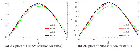
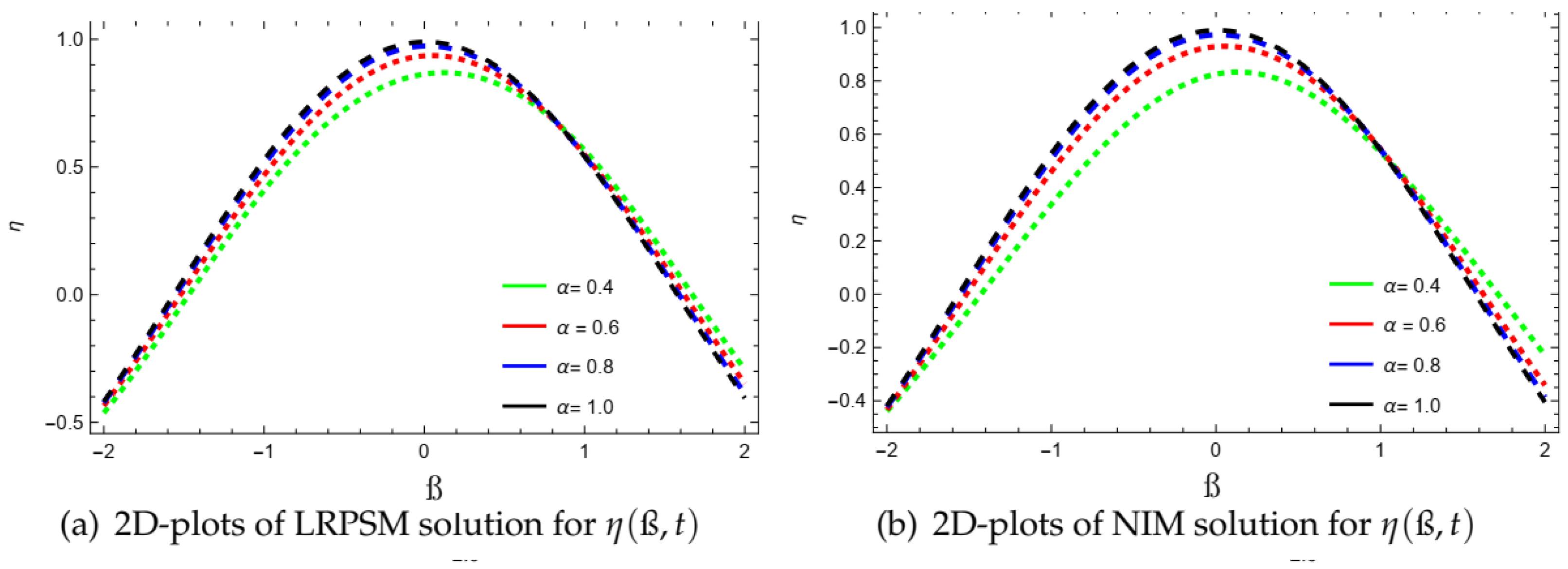
The figures presented in the discussion show the solutions of the fractional-order coupled Schrödinger–KdV equation using two different numerical methods: the LRPSM and NIM methods. Figure 3 shows 2D plots of the solutions for the wave function $\eta (ß,t)$, with subfigures (a) and (b) displaying the LRPSM and NIM methods, respectively. When the two methods are compared, they produce similar results, with the LRPSM method appearing to be slightly more accurate in this case. Figure 4 shows 3D plots of the solutions for $\eta (ß,t)$, with subfigures (a) and (b) displaying the LRPSM and NIM methods, respectively. The 3D plots provide a complete view of the solutions, displaying variations in the wave function over time and space. Again, the solutions obtained by the two methods are very similar, with the LRPSM method slightly more accurate.

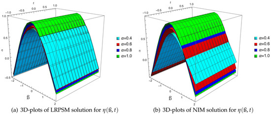
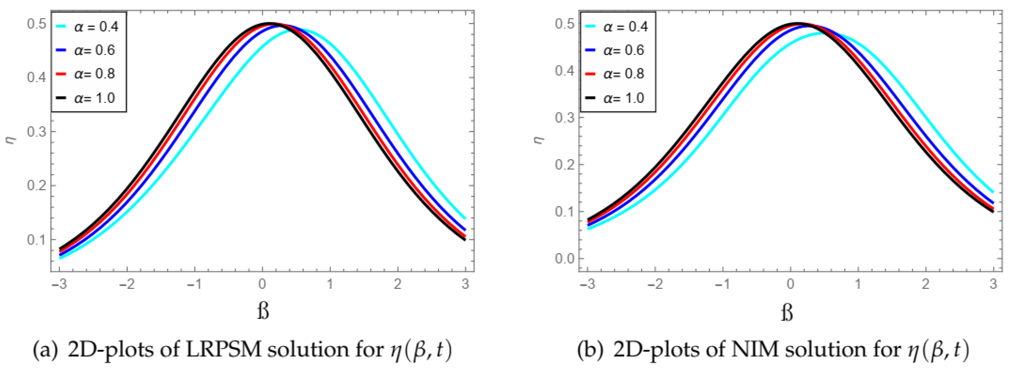
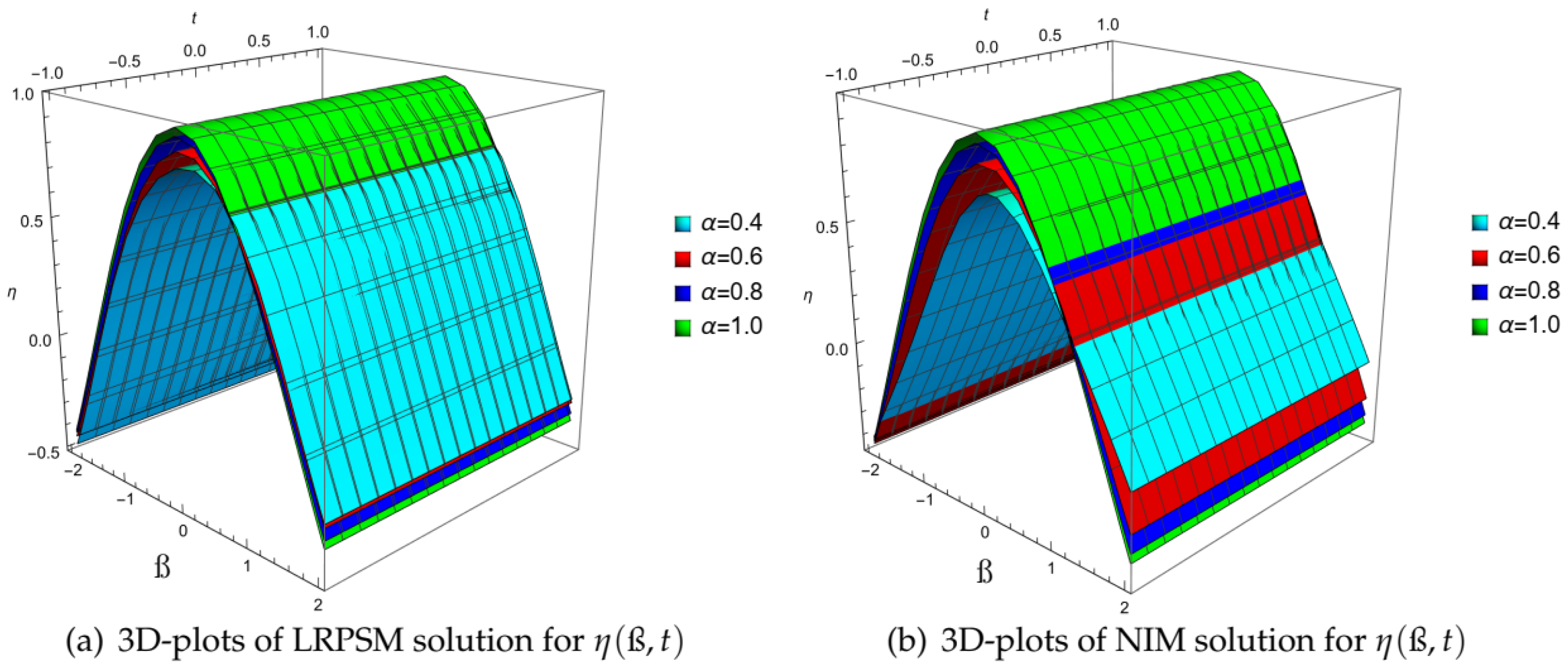
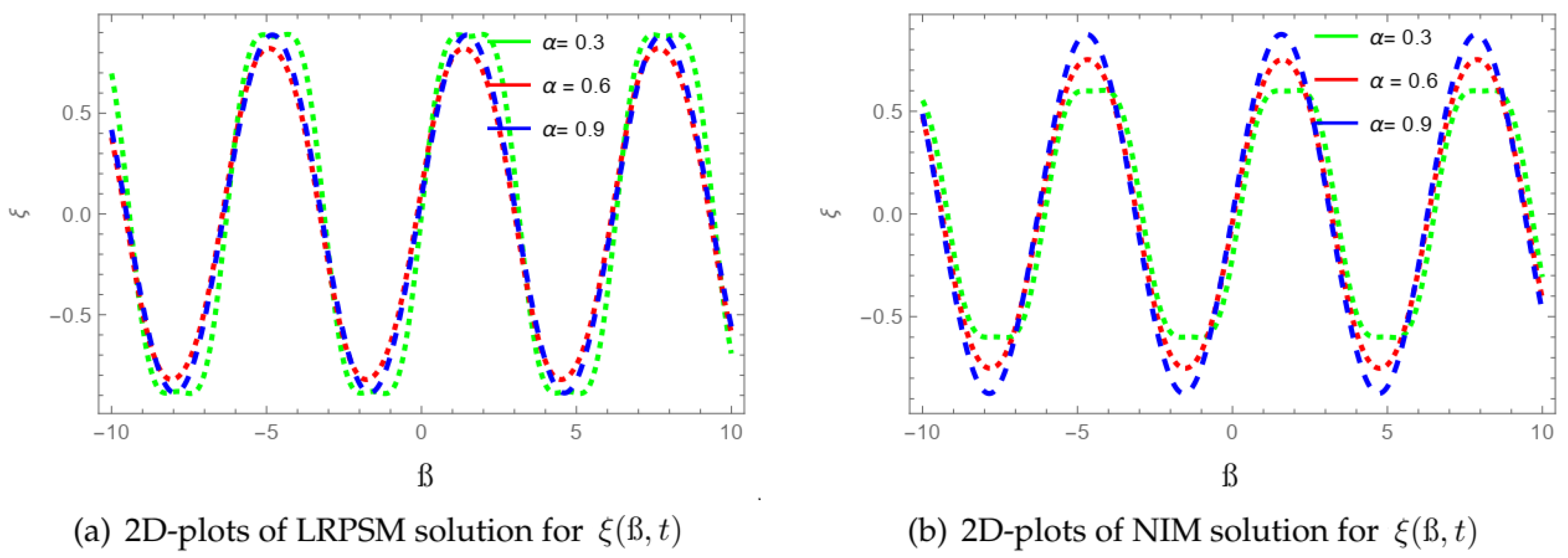
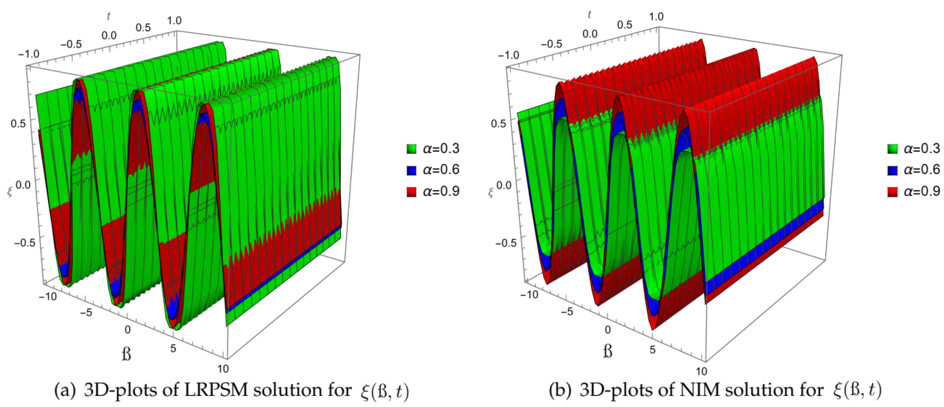
Figure 5 shows 2D plots of the solutions for the other variable in the equation $\xi (ß,t)$, with subfigures (a) and (b) displaying the LRPSM and NIM solutions, respectively. As previously stated, the two methods yield similar results, with the LRPSM method yielding slightly more accurate results. Finally, Figure 6 shows 3D plots of the solutions for $\xi (ß,t)$, with subfigures (a) and (b) displaying the LRPSM and NIM methods, respectively. Figure 7, 3D plots of LRPSM and NIM solutions of $\xi (ß,t)$ at various values of fractional order.

Table 3. Numerical values of $\eta (ß,t)$ by using NIM and LRPSM with dissimilar values of fractional orders $\alpha =0.4$, $\alpha =0.6$, and $\alpha =0.8$.

ß	${\mathit{NIM}}_{\mathit{\alpha }=0.4}$	${\mathit{LRPSM}}_{\mathit{\alpha }=0.4}$	${\mathit{NIM}}_{\mathit{\alpha }=0.6}$	${\mathit{LRPSM}}_{\mathit{\alpha }=0.6}$	${\mathit{NIM}}_{\mathit{\alpha }=0.8}$	${\mathit{LRPSM}}_{\mathit{\alpha }=0.8}$
0.1	−0.189874	−0.176482	−0.172736	−0.169667	−0.165132	−0.164485
0.2	−0.17988	−0.167194	−0.163645	−0.160737	−0.15644	−0.155828
0.3	−0.169887	−0.157905	−0.154553	−0.151807	−0.147749	−0.14717
0.4	−0.159894	−0.148617	−0.145462	−0.142877	−0.139058	−0.138513
0.5	−0.1499	−0.139328	−0.136371	−0.133948	−0.130367	−0.129856
0.6	−0.139907	−0.13004	−0.127279	−0.125018	−0.121676	−0.121199
0.7	−0.129914	−0.120751	−0.118188	−0.116088	−0.112985	−0.112542
0.8	−0.11992	−0.111463	−0.109096	−0.107158	−0.104294	−0.103885
0.9	−0.109927	−0.102174	−0.100005	−0.0982282	−0.0956025	−0.0952279
1	−0.0999335	−0.0928855	−0.0909137	−0.0892983	−0.0869114	−0.0865708

,

Table 4. Comparison of NIM and LRPSM solutions with the exact solution and absolute error for $\eta (ß,t)$.

ß	NIM	LRPSM	Exact	NIM Error	LRPSM Error	HPSTM Error [50]
0	0.991481	0.991556	0.999998	0.00851667	0.0084413	0.0084617
0.2	0.972981	0.97305	0.979642	0.00666104	0.00659231	0.00669431
0.4	0.915696	0.915755	0.920231	0.00453561	0.0044759	0.0045769
0.6	0.821906	0.821955	0.824134	0.00222747	0.00217903	0.00237503
0.8	0.695349	0.695384	0.695181	0.00016832	0.00020345	0.00021345
1	0.541067	0.541087	0.538513	0.00255363	0.00257369	0.00267168
1.2	0.365208	0.365212	0.360376	0.00483206	0.0048358	0.0039348
1.4	0.174786	0.174773	0.167873	0.00691323	0.0069001	0.0069231
1.6	−0.0226073	-0.022637	−0.0313235	0.00871626	0.00868658	0.00967657

and

Table 5. Comparison of NIM and LRPSM solutions with the exact solution and absolute error for $\eta (ß,t)$.

ß	NIM	LRPSM	Exact	NIM Error	LRPSM Error	HPSTM Error [50]
0	−0.0000270	0.0063208	0.002125	0.002152	0.004195	0.006295
0.2	0.196972	0.2032	0.200752	0.00377968	0.00244894	0.00256804
0.4	0.386115	0.391976	0.391375	0.0052597	0.00060127	0.00070134
0.6	0.55986	0.565119	0.566395	0.0065352	0.00127557	0.00138435
0.8	0.711279	0.715728	0.718835	0.00755558	0.00310701	0.00321702
1	0.834339	0.837799	0.842617	0.00827852	0.00481835	0.00471935
1.2	0.924135	0.926469	0.932807	0.00867223	0.00633839	0.00643939
1.4	0.977091	0.978205	0.985809	0.00871776	0.00760327	0.00780727
1.6	0.991098	0.990949	0.999509	0.00841091	0.00856015	0.00957010

compare the NIM and LRPSM solutions with the exact solution and the absolute error for $\eta (ß,t)$ and $\xi (ß,t)$. Again, the solutions obtained by the two methods are very similar, with the LRPSM method slightly more accurate. Overall, the figures provide a clear and informative comparison of the solutions obtained by the two numerical methods for the fractional-order coupled Schrödinger–KdV equation, highlighting similarities and differences and providing insight into the relative accuracy and effectiveness of the two methods.

5. Conclusions

In conclusion, we have presented two efficient methods for solving the fractional-order Schrödinger–KdV system: the Laplace residual power series method (LRPSM) and the new iterative method (NIM). Numerical experiments have demonstrated the accuracy and efficacy of both methods, which have been successfully applied to this challenging problem. The residual power series method entails expressing the solution as a power series and employing residual correction to improve the solution’s precision. In contrast, the new iterative method employs the Laplace transform to simplify the problem and obtain a recursive solution formula. Experiments on the fractional Schrödinger–KdV system have demonstrated that both approaches can generate highly accurate solutions. However, the new iterative method is more efficient regarding computational time and memory consumption. These methods can potentially be applied to additional complex physics and engineering problems, especially those involving fractional derivatives. Consequently, our work significantly contributes to applied mathematics and physics and paves the way for future research.

References

- Yavuz, M.; Sulaiman, T.A.; Yusuf, A.; Abdeljawad, T. The Schrodinger-KdV equation of fractional order with Mittag-Leffler nonsingular kernel. Alex. Eng. J. 2021, 60, 2715–2724. [Google Scholar] [CrossRef]
- Alshammari, S.; Al-Sawalha, M.M. Approximate analytical methods for a fractional-order nonlinear system of Jaulent-Miodek equation with energy-dependent Schrodinger potential. Fractal Fract. 2023, 7, 140. [Google Scholar] [CrossRef]
- Al-Sawalha, M.M.; Ababneh, O.Y.; Nonlaopon, K. Numerical analysis of fractional-order Whitham-Broer-Kaup equations with non-singular kernel operators. AIMS Math. 2023, 8, 308–2336. [Google Scholar] [CrossRef]
- Botmart, T.; Alotaibi, B.M.; El-Sherif, L.S.; El-Tantawy, S.A. A Reliable Way to Deal with the Coupled Fractional Korteweg-De Vries Equations within the Caputo Operator. Symmetry 2022, 14, 2452. [Google Scholar] [CrossRef]
- Alderremy, A.A.; Aly, S.; Fayyaz, R.; Khan, A.; Shah, R.; Wyal, N. The analysis of fractional-order nonlinear systems of third order KdV and Burgers equations via a novel transform. Complexity 2022, 2022, 4935809. [Google Scholar] [CrossRef]
- Yasmin, H.; Aljahdaly, N.H.; Saeed, A.M. Investigating Families of Soliton Solutions for the Complex Structured Coupled Fractional Biswas-Arshed Model in Birefringent Fibers Using a Novel Analytical Technique. Fractal Fract. 2023, 7, 491. [Google Scholar] [CrossRef]
- Yasmin, H.; Aljahdaly, N.H.; Saeed, A.M.; Shah, R. Investigating Symmetric Soliton Solutions for the Fractional Coupled Konno-Onno System Using Improved Versions of a Novel Analytical Technique. Mathematics 2023, 11, 2686. [Google Scholar] [CrossRef]
- Lyu, W.; Wang, Z. Global classical solutions for a class of reaction-diffusion system with density-suppressed motility. Electron. Res. Arch. 2022, 30, 995–1015. [Google Scholar] [CrossRef]
- He, H.M.; Peng, J.G.; Li, H.Y. Iterative approximation of fixed point problems and variational inequality problems on Hadamard manifolds. UPB Bull. Ser. A 2022, 84, 25–36. [Google Scholar]
- He, H.; Peng, J.; Li, H. Implicit viscosity iterative algorithm for nonexpansive mapping on Hadamard manifolds. Fixed Point Theory 2023, 24, 213–220. [Google Scholar] [CrossRef]
- Zhang, X.; Lu, Z.; Yuan, X.; Wang, Y.; Shen, X. L2-Gain Adaptive Robust Control for Hybrid Energy Storage System in Electric Vehicles. IEEE Trans. Power Electron. 2021, 36, 7319–7332. [Google Scholar] [CrossRef]
- Wang, B.; Zhang, Y.; Zhang, W. A Composite Adaptive Fault-Tolerant Attitude Control for a Quadrotor UAV with Multiple Uncertainties. J. Syst. Sci. Complex. 2022, 35, 81–104. [Google Scholar] [CrossRef]
- Li, Q.; Lin, H.; Tan, X.; Du, S. H ∞ Consensus for Multiagent-Based Supply Chain Systems Under Switching Topology and Uncertain Demands. IEEE Trans. Syst. Man, Cybern. Syst. 2020, 50, 4905–4918. [Google Scholar] [CrossRef]
- Mi, C.; Huang, S.; Zhang, Y.; Zhang, Z.; Postolache, O. Design and Implementation of 3-D Measurement Method for Container Handling Target. J. Mar. Sci. Eng. 2022, 10, 1961. [Google Scholar] [CrossRef]
- Xiao, Y.; Zhang, Y.; Kaku, I.; Kang, R.; Pan, X. Electric vehicle routing problem: A systematic review and a new comprehensive model with nonlinear energy recharging and consumption. Renew. Sustain. Energy Rev. 2021, 151, 111567. [Google Scholar] [CrossRef]
- Guo, C.; Hu, J. Fixed-Time Stabilization of High-Order Uncertain Nonlinear Systems: Output Feedback Control Design and Settling Time Analysis. J. Syst. Sci. Complex. 2023, 36, 1351–1372. [Google Scholar] [CrossRef]
- Guo, C.; Hu, J.; Hao, J.; Celikovsky, S.; Hu, X. Fixed-time safe tracking control of uncertain high-order nonlinear pure-feedback systems via unified transformation functions. Kybernetika 2023, 59, 342–364. [Google Scholar] [CrossRef]
- Lee, Y.Y.; Tang, T.K.; Phuah, E.T.; Lai, O.M. Recent Advances in Edible Fats and Oils Technology: Processing, Health Implications, Economic and Environmental Impact; Springer: Singapore, 2022. [Google Scholar]
- Zhang, T.; Li, Y. Global exponential stability of discrete-time almost automorphic Caputo-Fabrizio BAM fuzzy neural networks via exponential Euler technique. Knowl.-Based Syst. 2022, 246, 108675. [Google Scholar] [CrossRef]
- Shafee, A.; Alkhezi, Y. Efficient Solution of Fractional System Partial Differential Equations Using Laplace Residual Power Series Method. Fractal Fract. 2023, 7, 429. [Google Scholar] [CrossRef]
- Mainardi, F.; Luchko, Y.; Pagnini, G. The fundamental solution of the space-time fractional diffusion equation. arXiv 2007, arXiv:cond-mat/0702419. [Google Scholar]
- Miller, K.S.; Ross, B. An Introduction to the Fractional Calculus and Fractional Differential Equations; Wiley: Hoboken, NJ, USA, 1993. [Google Scholar]
- Alshehry, A.S.; Yasmin, H.; Ghani, F.; Shah, R.; Nonlaopon, K. Comparative Analysis of Advection-Dispersion Equations with Atangana-Baleanu Fractional Derivative. Symmetry 2023, 15, 819. [Google Scholar] [CrossRef]
- Tarasov, V.E. On history of mathematical economics: Application of fractional calculus. Mathematics 2019, 7, 509. [Google Scholar] [CrossRef]
- Yasmin, H.; Alshehry, A.S.; Saeed, A.M.; Nonlaopon, K. Application of the q-Homotopy Analysis Transform Method to Fractional-Order Kolmogorov and Rosenau-Hyman Models within the Atangana-Baleanu Operator. Symmetry 2023, 15, 671. [Google Scholar] [CrossRef]
- Tarasov, V.E. Fractional Dynamics: Applications of Fractional Calculus to Dynamics of Particles, Fields and Media; Springer Science & Business Media: Berlin/Heidelberg, Germany, 2011. [Google Scholar]
- Bronski, J.C.; Carr, L.D.; Deconinck, B.; Kutz, J.N. Bose-Einstein condensates in standing waves: The cubic nonlinear Schrodinger equation with a periodic potential. Phys. Rev. Lett. 2001, 86, 1402. [Google Scholar] [CrossRef] [PubMed]
- Trombettoni, A.; Smerzi, A. Discrete solitons and breathers with dilute Bose-Einstein condensates. Phys. Lett. 2001, 86, 2353. [Google Scholar] [CrossRef]
- Triki, H.; Biswas, A. Dark solitons for a generalized nonlinear Schrodinger equation with parabolic law and dual-power law nonlinearities. Math. Methods Appl. Sci. 2011, 34, 958–962. [Google Scholar] [CrossRef]
- Zhang, L.H.; Si, J.G. New soliton and periodic solutions of (1+ 2)-dimensional nonlinear Schrodinger equation with dual-power law nonlinearity. Commun. Nonlinear Sci. Numer. Simul. 2010, 15, 2747–2754. [Google Scholar] [CrossRef]
- Nore, C.; Brachet, M.; Fauve, S. Numerical study of hydrodynamics using the nonlinear Schrodinger equation. Phys. D Nonlinear Phenom. 1993, 65, 154–162. [Google Scholar] [CrossRef]
- Burqan, A.; El-Ajou, A.; Saadeh, R.; Al-Smadi, M. A new efficient technique using Laplace transforms and smooth expansions to construct a series solution to the time-fractional Navier-Stokes equations. AlexandriaEng. J. 2022, 61, 1069–1077. [Google Scholar] [CrossRef]
- Khater, M.M.; Attia, R.A.; Lu, D. Numerical solutions of nonlinear fractional Wu-Zhang system for water surface versus three approximate schemes. J. Ocean Eng. Sci. 2019, 4, 144–148. [Google Scholar] [CrossRef]
- Veeresha, P.; Prakasha, D.; Magesh, N.; Nandeppanavar, M.; Christopher, A.J. Numerical simulation for fractional Jaulent-Miodek equation associated with energy-dependent Schrodinger potential using two novel techniques. Waves Random Complex Media 2021, 31, 1141–1162. [Google Scholar] [CrossRef]
- Singh, J.; Kumar, D.; Baleanu, D.; Rathore, S. On the local fractional wave equation in fractal strings. Math. Methods Appl. Sci. 2019, 42, 1588–1595. [Google Scholar] [CrossRef]
- El-Ajou, A. Adapting the Laplace transform to create solitary solutions for the nonlinear time-fractional dispersive PDEs via a new approach. Eur. Phys. J. Plus 2021, 136, 229. [Google Scholar] [CrossRef]
- El-Ajou, A.; Al-Smadi, M.; Moaath, N.O.; Momani, S.; Hadid, S. Smooth expansion to solve high-order linear conformable fractional PDEs via residual power series method: Applications to physical and engineering equations. Ain Shams Eng. J. 2020, 11, 1243–1254. [Google Scholar] [CrossRef]
- El-Ajou, A.; Moaath, N.O.; Al-Zhour, Z.; Momani, S. A class of linear non-homogenous higher order matrix fractional differential equations: Analytical solutions and new technique. Fract. Calc. Appl. Anal. 2020, 23, 356–377. [Google Scholar] [CrossRef]
- Aljahdaly, N.H.; Akgul, A.; Shah, R.; Mahariq, I.; Kafle, J. A comparative analysis of the fractional-order coupled Korteweg-De Vries equations with the Mittag-Leffler law. J. Math. 2022, 2022, 8876149. [Google Scholar] [CrossRef]
- El-Ajou, A.; Al-Zhour, Z.; Oqielat, M.; Momani, S.; Hayat, T. Series solutions of nonlinear conformable fractional KdV-Burgers equation with some applications. Eur. Phys. J. Plus 2019, 134, 402. [Google Scholar] [CrossRef]
- Moaath, N.O.; El-Ajou, A.; Al-Zhour, Z.; Alkhasawneh, R.; Alrabaiah, H. Series solutions for nonlinear time-fractional Schrodinger equations: Comparisons between conformable and Caputo derivatives. Alex. Eng. J. 2020, 59, 2101–2114. [Google Scholar]
- Benchohra, M.; Cabada, A.; Seba, D. An existence result for nonlinear fractional differential equations on Banach spaces. Bound. Value Probl. 2009, 2009, 628916. [Google Scholar] [CrossRef]
- Areshi, M.; Khan, A.; Shah, R.; Nonlaopon, K. Analytical investigation of fractional-order Newell-Whitehead-Segel equations via a novel transform. Aims Math. 2022, 7, 6936–6958. [Google Scholar] [CrossRef]
- Arqub, O.A.; El-Ajou, A.; Momani, S. Constructing and predicting solitary pattern solutions for nonlinear time-fractional dispersive partial differential equations. J. Comput. Phys. 2015, 293, 385–399. [Google Scholar] [CrossRef]
- Li, C.; Qian, D.; Chen, Y. On Riemann-Liouville and caputo derivatives. Discret. Dyn. Nat. Society 2011, 2011, 562494. [Google Scholar] [CrossRef]
- Kexue, L.; Jigen, P. Laplace transform and fractional differential equations. Appl. Math. Lett. 2011, 24, 2019–2023. [Google Scholar] [CrossRef]
- Daftardar-Gejji, V.; Jafari, H. An iterative method for solving nonlinear functional equations. J. Ofmath. Anal. Appl. 2006, 316, 753–763. [Google Scholar] [CrossRef]
- Hemeda, A. New iterative method: Application to nth-order integro-differential equations. Int. Forum 2012, 7, 2317–2332. [Google Scholar]
- Momani, S. An explicit and numerical solutions of the fractional KdV equation. Math. Comput. Simul. 2005, 70, 110–118. [Google Scholar] [CrossRef]
- Shah, R.; Hyder, A.A.; Iqbal, N.; Botmart, T. Fractional view evaluation system of Schrodinger-KdV equation by a comparative analysis. AIMS Math. 2022, 7, 19846–19864. [Google Scholar] [CrossRef]
Disclaimer/Publisher’s Note: The statements, opinions and data contained in all publications are solely those of the individual author(s) and contributor(s) and not of MDPI and/or the editor(s). MDPI and/or the editor(s) disclaim responsibility for any injury to people or property resulting from any ideas, methods, instructions or products referred to in the content. |
© 2023 by the author. Licensee MDPI, Basel, Switzerland. This article is an open access article distributed under the terms and conditions of the Creative Commons Attribution (CC BY) license (https://creativecommons.org/licenses/by/4.0/).