


Reliability Analysis of Kavya Manoharan Kumaraswamy Distribution under Generalized Progressive Hybrid Data


Abstract
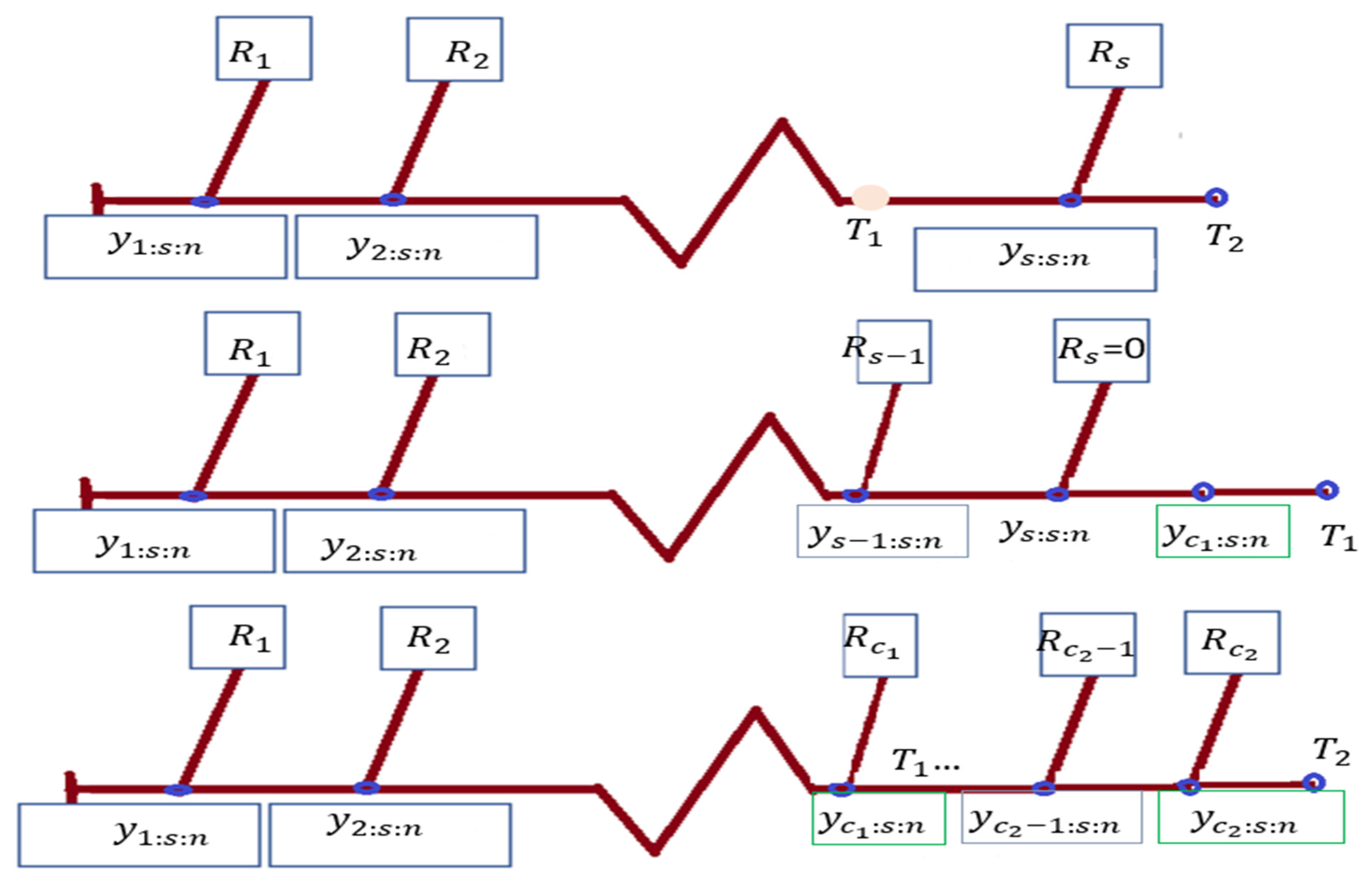
:1. Introduction
- With setting to 0, use PHCS-T1.
- . by setting PHCS-T2.
- You may do hybrid type-I censoring by setting .
- , can be used to do hybrid type-II censoring.
- To do type-I censoring, set
- A type-II censored sample is produced by setting
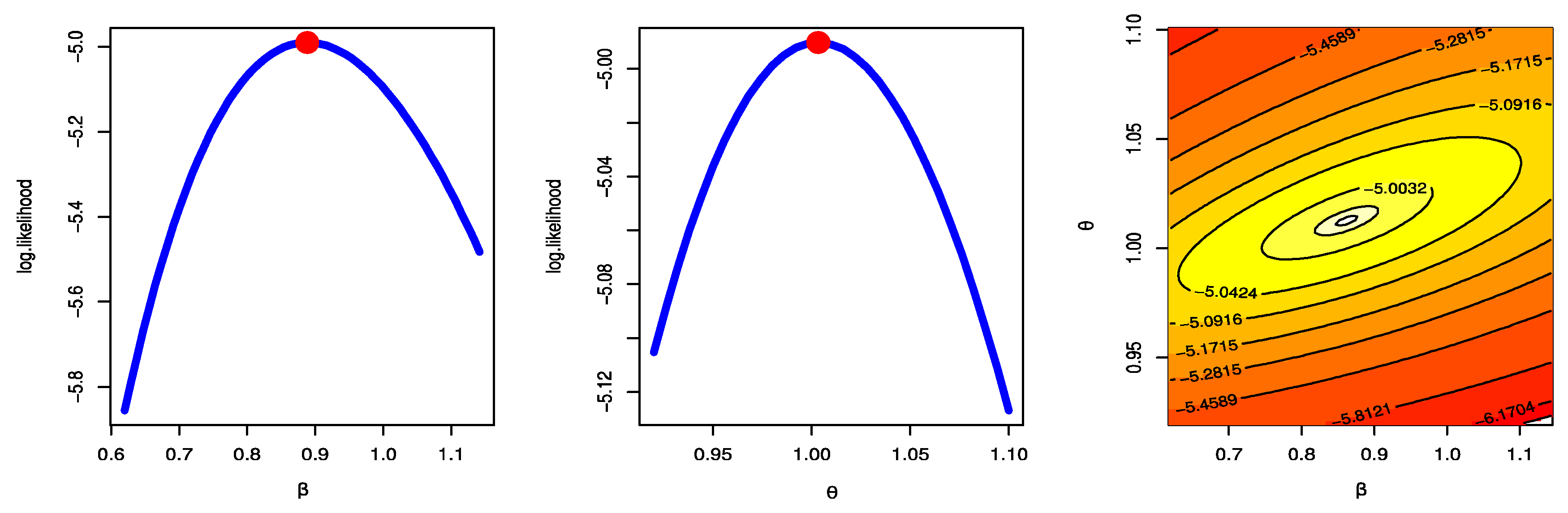
2. Likelihood Estimation
3. Bayes Estimator
- We believe the main motivation for the gamma prior is usually to constrain the random variables to positive values.
- The gamma distribution is considered one of the most important and well-known statistical distributions because it is compatible with many engineering, mathematical, statistical, and medical applications.
- The gamma distribution is one of the most famous distributions that is used in mathematical solutions (integrations), especially when the data are from 0 to ∞.
- In previous studies, the gamma distribution was the most popular prior distribution and was associated with the best statistical results.
4. Interval Estimators
4.1. Asymptotic Intervals
4.2. HPD Intervals
5. Optimal PCS-T2 Designs
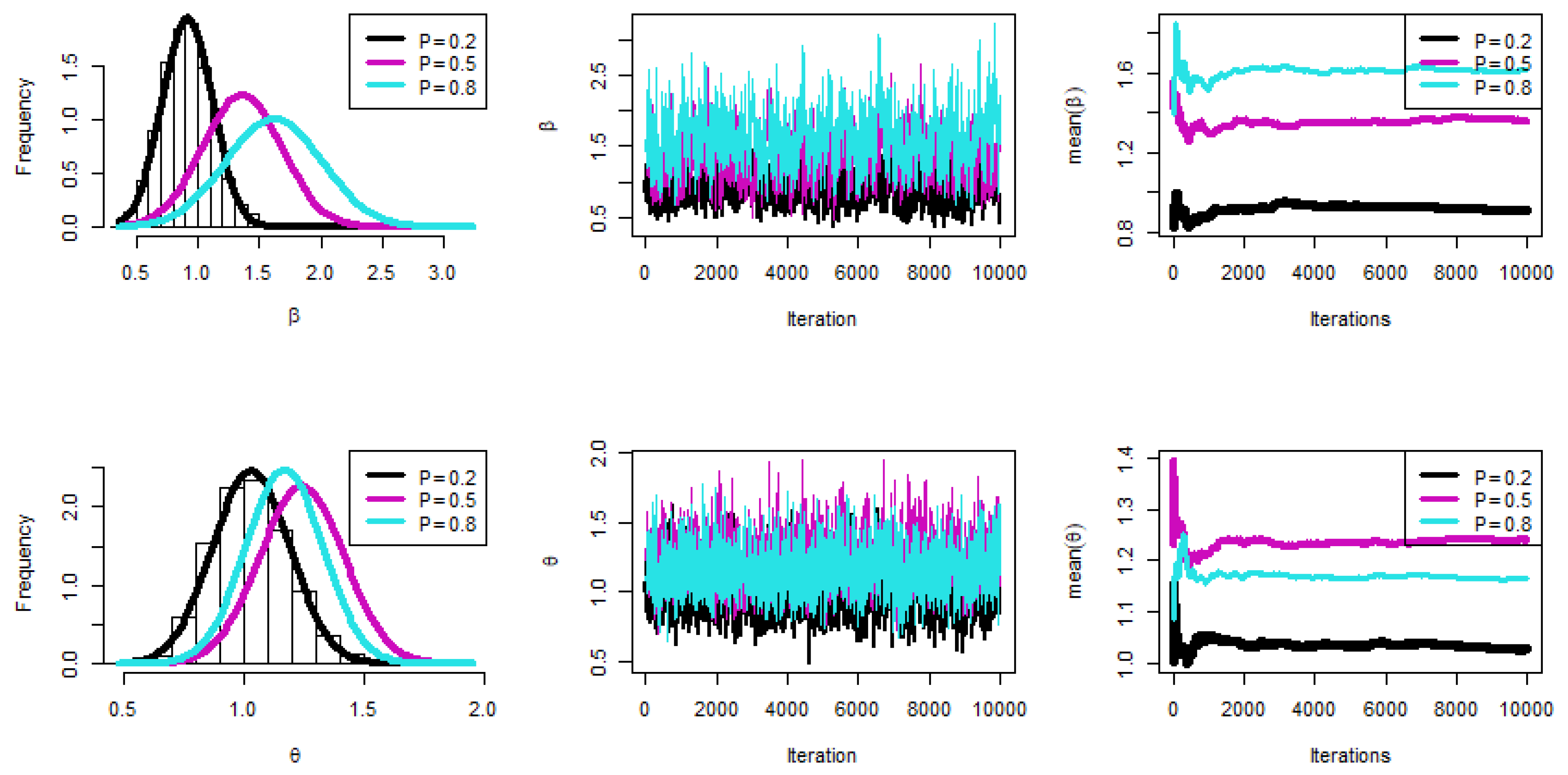
6. Simulation
- The key general finding is that the suggested values for and performed well.
- All estimations of R(t), and h(t) functioned satisfactorily as n(or s) grew.
- In most cases, the MSE, Bias, and WCI of all unknown parameters fell while their CPs grew as (T1, T2) increased.
- Due to the gamma information, the Bayes estimates of and behaved more predictably than the other estimates. Regarding credible HPD intervals, the same statement might be made.
- When the parameter of binomial r was increased, the proposed estimates of and performed better in most cases.
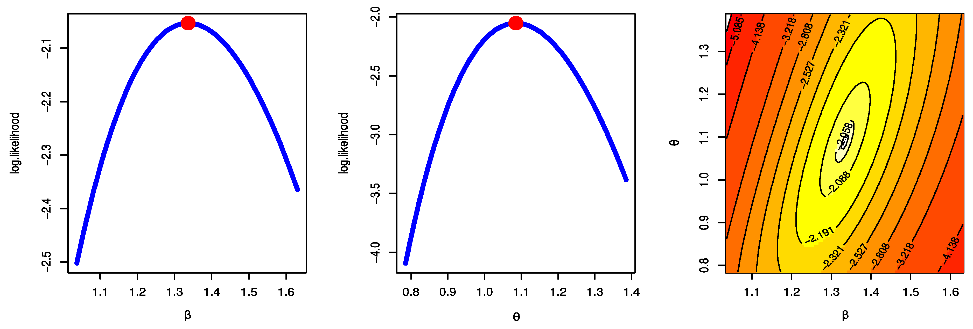
7. Application
8. Conclusions and Discussion
- The key general finding is that the suggested values for and performed well.
- All estimations of R(t), and h(t) functioned satisfactorily as n (or s) grew.
- In most cases, the MSE, Bias, and WCI of all unknown parameters fell while their CPs grew as (T1, T2) increased.
- Due to the gamma information, the Bayes estimates of and behaved more predictably than the other estimates. Regarding credible HPD intervals, the same statement might be made.
- In most cases, the proposed estimates of and performed better when the parameter of binomial was increased.
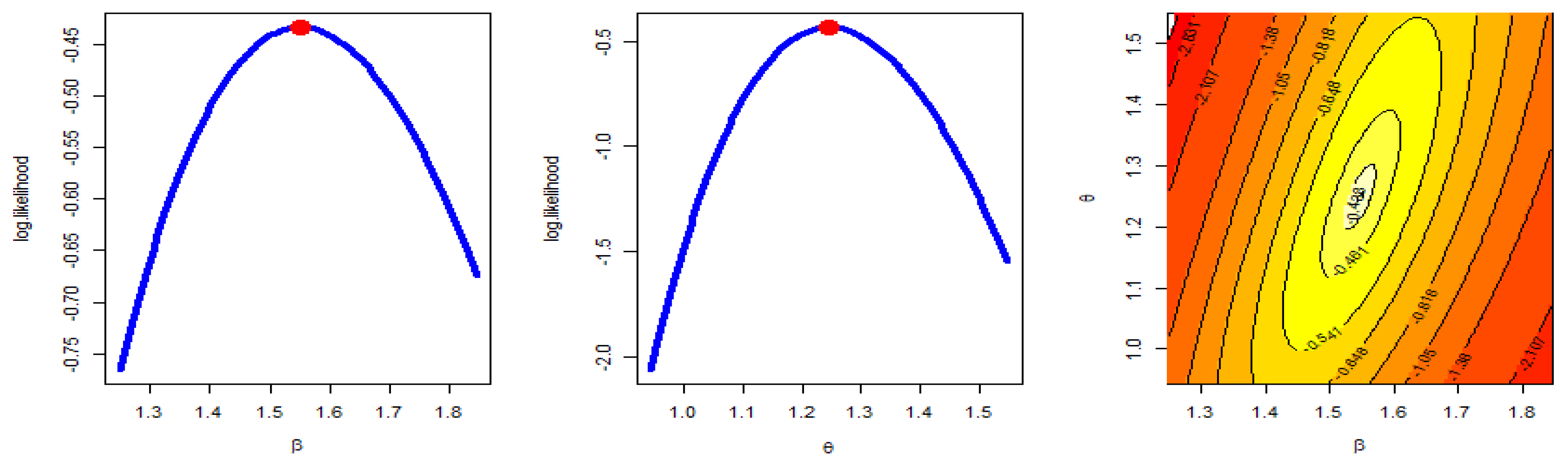
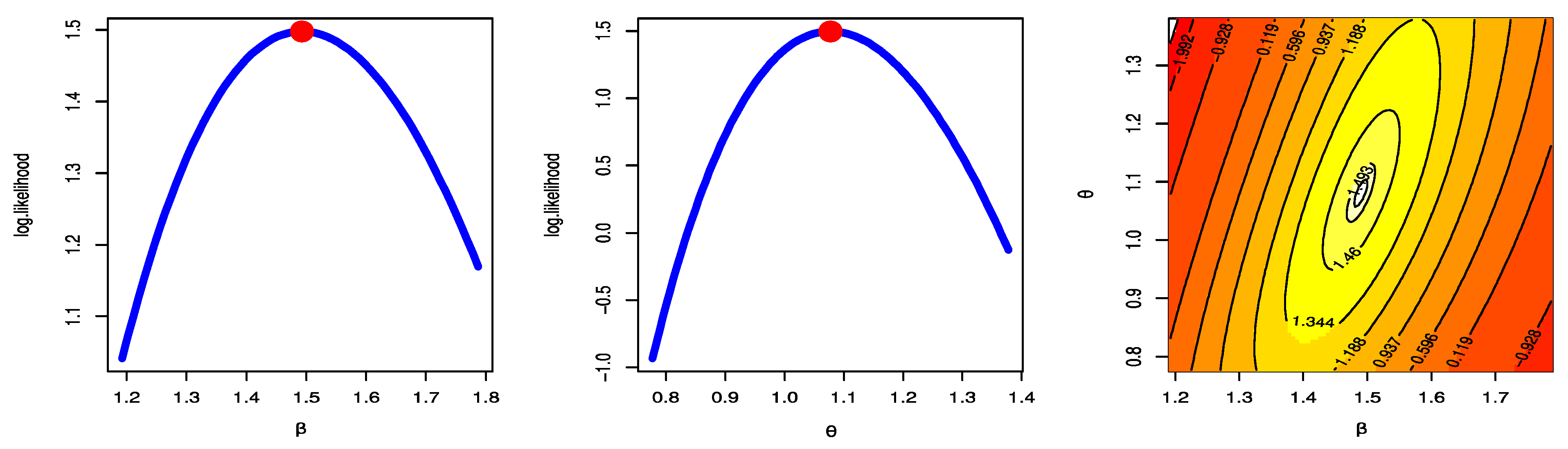
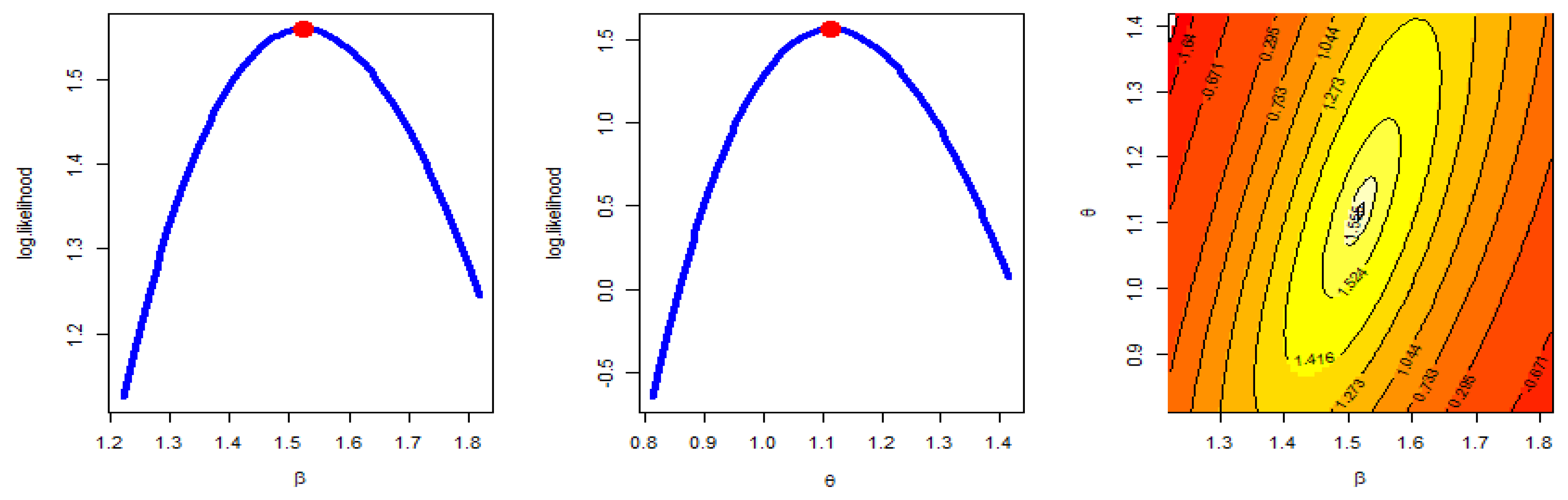
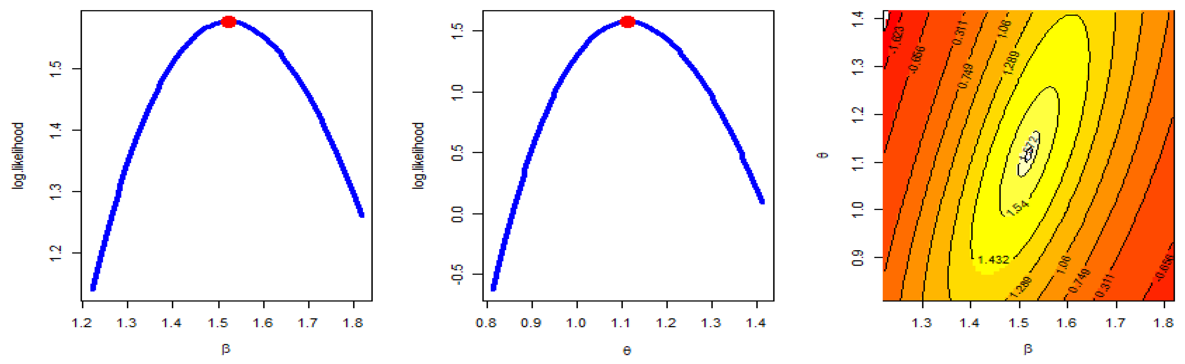
- The MLE has a unique solution and a maximum value of log-likelihood.
Author Contributions
Funding
Institutional Review Board Statement
Informed Consent Statement
Data Availability Statement
Acknowledgments
Conflicts of Interest
References
- Balakrishnan, N.; Aggarwala, R. Progressive Censoring: Theory, Methods, and Applications; Springer Science & Business Media: Berlin, Germany, 2000. [Google Scholar]
- Balakrishnan, N. Progressive censoring methodology: An appraisal. TEST 2007, 16, 211–259. [Google Scholar] [CrossRef]
- Balakrishnan, N.; Cramer, E. The Art of Progressive Censoring; Springer: New York, NY, USA, 2014. [Google Scholar]
- Kundu, D.; Joarder, A. Analysis of Type-II progressively hybrid censored data. Comput. Stat. Data Anal. 2006, 50, 2509–2528. [Google Scholar] [CrossRef]
- Childs, A.; Chandrasekar, B.; Balakrishnan, N. Exact likelihood inference for an exponential parameter under progressive hybrid censoring schemes. In Statistical Models and Methods for Biomedical and Technical Systems; Vonta, F., Nikulin, M., Limnios, N., Huber-Carol, C., Eds.; Birkhäuser: Boston, MA, USA, 2008; pp. 319–330. [Google Scholar]
- Lee, K.; Sun, H.; Cho, Y. Exact likelihood inference of the exponential parameter under generalized Type II progressive hybrid censoring. J. Korean Stat. Soc. 2016, 45, 123–136. [Google Scholar] [CrossRef]
- Ateya, S.; Mohammed, H. Prediction under Burr-XII distribution based on generalized Type-II progressive hybrid censoring scheme. J. Egypt. Math. Soc. 2018, 26, 491–508. [Google Scholar]
- Seo, J.I. Objective Bayesian analysis for the Weibull distribution with partial information under the generalized Type-II progressive hybrid censoring scheme. Commun. Stat.-Simul. Comput. 2020, 51, 5157–5173. [Google Scholar] [CrossRef]
- Cho, S.; Lee, K. Exact likelihood inference for a competing risks model with generalized Type-II progressive hybrid censored exponential data. Symmetry 2021, 13, 887. [Google Scholar] [CrossRef]
- Nagy, M.; Bakr, M.E.; Alrasheedi, A.F. Analysis with applications of the generalized Type-II progressive hybrid censoring sample from Burr Type-XII model. Math. Probl. Eng. 2022, 2022, 1241303. [Google Scholar] [CrossRef]
- Alotaibi, N.; Elbatal, I.; Shrahili, M.; Al-Moisheer, A.S.; Elgarhy, M.; Almetwally, E.M. Statistical Inference for the Kavya–Manoharan Kumaraswamy Model under Ranked Set Sampling with Applications. Symmetry 2023, 15, 587. [Google Scholar] [CrossRef]
- Henningsen, A.; Toomet, O. maxlik: A package for maximum likelihood estimation in R. Comput Stat. 2011, 26, 443–458. [Google Scholar] [CrossRef]
- Plummer, M.; Best, N.; Cowles, K.; Vines, K. CODA: Convergence diagnosis and output analysis for MCMC. RNews 2006, 6, 7–11. [Google Scholar]
- Luo, C.; Shen, L.; Xu, A. Modelling and estimation of system reliability under dynamic operating environments and lifetime ordering constraints. Reliab. Eng. Syst. Saf. 2022, 218, 108136. [Google Scholar] [CrossRef]
- Shirong, Z.; Ancha, X.; Yincai, T.; Lijuan, S. Fast Bayesian Inference of Reparameterized Gamma Process with Random Effects. IEEE Trans. Reliab. 2023, 1–14. [Google Scholar] [CrossRef]
- Zhuang, L.; Xu, A.; Wang, X.-L. A prognostic driven predictive maintenance framework based on Bayesian deep learning. Reliab. Eng. Syst. Saf. 2023, 234, 109181. [Google Scholar] [CrossRef]
- Gelman, A.; Carlin, J.B.; Stern, H.S.; Rubin, D.B. Bayesian Data Analysis, 2nd ed.; Chapman and Hall/CRC: Boca Raton, FL, USA, 2004. [Google Scholar]
- Lynch, S.M. Introduction to Applied Bayesian Statistics and Estimation for Social Scientists; Springer: New York, NY, USA, 2007. [Google Scholar]
- Lawless, J.F. Statistical Models and Methods for Lifetime Data, 2nd ed.; John Wiley and Sons: Hoboken, NJ, USA, 1982. [Google Scholar]
- Greene, W.H. Econometric Analysis, 4th ed.; Prentice-Hall: New York, NY, USA, 2000. [Google Scholar]
- Chen, M.H.; Shao, Q.M. Monte Carlo estimation of Bayesian credible and HPD intervals. J. Comput. Graph. Stat. 1999, 8, 69–92. [Google Scholar]
- Ng, H.K.T.; Chan, P.S.; Balakrishnan, N. Optimal progressive censoring plans for the Weibull distribution. Technometrics 2004, 46, 470–481. [Google Scholar] [CrossRef]
- Pradhan, B.; Kundu, D. Inference and optimal censoring schemes for progressively censored Birnbaum–Saunders distribution. J. Stat. Plan. Inference 2013, 143, 1098–1108. [Google Scholar] [CrossRef]
- Alotaibi, R.; Mutairi, A.; Almetwally, E.M.; Park, C.; Rezk, H. Optimal Design for a Bivariate Step-Stress Accelerated Life Test with Alpha Power Exponential Distribution Based on Type-I Progressive Censored Samples. Symmetry 2022, 14, 830. [Google Scholar] [CrossRef]
- Dey, S.; Singh, S.; Tripathi, Y.M.; Asgharzadeh, A. Estimation and prediction for a progressively censored generalized inverted exponential distribution. Stat. Methodol. 2016, 32, 185–202. [Google Scholar]


| 1 | ||||
| 2 | s | 1 | 0 | |
| 3 |
| Criterion | Method |
|---|---|
| Maximize trace | |
| Minimize trace | |
| Minimize det | |
| Minimize |
| MLE | Bayesian | |||||||||||
|---|---|---|---|---|---|---|---|---|---|---|---|---|
| n | r | s | Bias | MSE | WACI | CP | Optimality | Bias | MSE | WCCI | ||
| 30 | 0.3 | 20 | 0.3647 | 0.96096 | 3.5687 | 95.8% | 0.862132 | 0.0495 | 0.03658 | 0.9815 | ||
| 0.3083 | 0.30741 | 1.8074 | 95.3% | 0.050431 | 0.0652 | 0.0178 | 0.6268 | |||||
| R(0.6) | −1.0730 | 0.01021 | 3.5687 | 95.8% | 24.39956 | −1.0929 | 0.00159 | 0.9815 | ||||
| H(0.6) | 2.6011 | 2.15503 | 1.8074 | 95.3% | 0.397259 | 2.2794 | 0.15897 | 0.6268 | ||||
| R(0.85) | −1.3190 | 0.00311 | 3.5687 | 95.8% | −1.3269 | 0.00026 | 0.9815 | |||||
| H(0.85) | 9.8905 | 28.98923 | 1.8074 | 95.3% | 8.2579 | 1.30669 | 0.6268 | |||||
| 25 | 0.3133 | 0.68518 | 3.0049 | 96.0% | 0.603238 | 0.0348 | 0.01182 | 0.6606 | ||||
| 0.1931 | 0.20528 | 1.6075 | 95.7% | 0.028622 | 0.0196 | 0.00163 | 0.4069 | |||||
| R(0.6) | −1.0962 | 0.00644 | 3.0049 | 96.0% | 29.16632 | −1.1016 | 0.00050 | 0.6606 | ||||
| H(0.6) | 2.6177 | 1.64301 | 1.6075 | 95.7% | 0.637278 | 2.2792 | 0.05406 | 0.4069 | ||||
| R(0.85) | −1.3278 | 0.00190 | 3.0049 | 96.0% | −1.3295 | 0.00009 | 0.6606 | |||||
| H(0.85) | 9.6683 | 20.97684 | 1.6075 | 95.7% | 8.1852 | 0.42306 | 0.4069 | |||||
| 0.8 | 20 | 0.4478 | 1.11270 | 3.7458 | 95.6% | 0.897504 | 0.0686 | 0.04368 | 1.0098 | |||
| 0.2881 | 0.29977 | 1.8260 | 95.3% | 0.054545 | 0.0541 | 0.00853 | 0.6131 | |||||
| R(0.6) | −1.0925 | 0.00827 | 3.7458 | 95.6% | 23.77178 | −1.0994 | 0.00147 | 1.0098 | ||||
| H(0.6) | 2.7704 | 2.38574 | 1.8260 | 95.3% | 0.410967 | 2.3269 | 0.17886 | 0.6131 | ||||
| R(0.85) | −1.3285 | 0.00217 | 3.7458 | 95.6% | −1.3295 | 0.00025 | 1.0098 | |||||
| H(0.85) | 10.3764 | 33.31616 | 1.8260 | 95.3% | 8.3746 | 1.53529 | 0.6131 | |||||
| 25 | 0.3005 | 0.65995 | 2.9601 | 96.2% | 0.588428 | 0.0312 | 0.00897 | 0.6494 | ||||
| 0.1892 | 0.20103 | 1.5942 | 95.3% | 0.02822 | 0.0199 | 0.00162 | 0.4063 | |||||
| R(0.6) | −1.0954 | 0.00634 | 2.9601 | 96.2% | 28.83162 | −1.1009 | 0.00041 | 0.6494 | ||||
| H(0.6) | 2.5961 | 1.54340 | 1.5942 | 95.3% | 0.290327 | 2.2713 | 0.04112 | 0.4063 | ||||
| R(0.85) | −1.3273 | 0.00191 | 2.9601 | 96.2% | −1.3293 | 0.00008 | 0.6494 | |||||
| H(0.85) | 9.5939 | 20.02147 | 1.5942 | 95.3% | 8.1634 | 0.31889 | 0.4063 | |||||
| 50 | 0.3 | 35 | 0.2321 | 0.33855 | 2.0926 | 95.2% | 0.3524 | 0.0219 | 0.00682 | 0.2936 | ||
| 0.2206 | 0.16385 | 1.3310 | 94.8% | 0.0109 | 0.0389 | 0.00404 | 0.1817 | |||||
| R(0.6) | 0.0150 | 0.00491 | 0.2684 | 94.9% | 40.4391 | 0.0044 | 0.00056 | 0.0984 | ||||
| H(0.6) | 0.2660 | 0.86775 | 3.5013 | 95.4% | 0.4010 | 0.0230 | 0.03428 | 0.7479 | ||||
| R(0.85) | 0.0019 | 0.00151 | 0.1522 | 95.8% | 0.0005 | 0.00010 | 0.0418 | |||||
| H(0.85) | 1.2233 | 10.31472 | 11.6464 | 95.4% | 0.1173 | 0.24180 | 1.8061 | |||||
| 45 | 0.1009 | 0.17989 | 1.6157 | 95.3% | 0.2308 | 0.0127 | 0.00185 | 0.1390 | ||||
| 0.0688 | 0.07292 | 1.0241 | 95.5% | 0.0051 | 0.0080 | 0.00043 | 0.0697 | |||||
| R(0.6) | 0.0038 | 0.00306 | 0.2163 | 95.2% | 52.6779 | −0.0009 | 0.00013 | 0.0468 | ||||
| H(0.6) | 0.1237 | 0.55947 | 2.8931 | 95.4% | 0.3850 | 0.0228 | 0.00944 | 0.3526 | ||||
| R(0.85) | 0.0023 | 0.00099 | 0.1228 | 95.9% | −0.0008 | 0.00002 | 0.0202 | |||||
| H(0.85) | 0.5401 | 5.79962 | 9.2044 | 95.3% | 0.0729 | 0.06640 | 0.8489 | |||||
| 0.8 | 35 | 0.2292 | 0.33120 | 2.0704 | 95.7% | 0.3413 | 0.0302 | 0.00762 | 0.2866 | |||
| 0.1710 | 0.13353 | 1.2666 | 94.8% | 0.0103 | 0.0289 | 0.00277 | 0.1549 | |||||
| R(0.6) | 0.0043 | 0.00413 | 0.2516 | 94.5% | 40.8715 | 0.0003 | 0.00049 | 0.0905 | ||||
| H(0.6) | 0.2984 | 0.88222 | 3.4929 | 95.3% | 0.5510 | 0.0472 | 0.03668 | 0.6994 | ||||
| R(0.85) | −0.0013 | 0.00132 | 0.1424 | 95.8% | −0.0010 | 0.00009 | 0.0382 | |||||
| H(0.85) | 1.2328 | 10.27127 | 11.6023 | 95.7% | 0.1697 | 0.26968 | 1.7342 | |||||
| 45 | 0.1024 | 0.17088 | 1.6527 | 95.8% | 0.2313 | 0.0132 | 0.00183 | 0.1361 | ||||
| 0.0614 | 0.07091 | 1.0767 | 95.4% | 0.0052 | 0.0077 | 0.00047 | 0.0735 | |||||
| R(0.6) | 0.0020 | 0.00301 | 0.2196 | 95.0% | 52.8830 | −0.0011 | 0.00013 | 0.0450 | ||||
| H(0.6) | 0.1288 | 0.55691 | 2.9153 | 95.4% | 0.3953 | 0.0242 | 0.00934 | 0.3352 | ||||
| R(0.85) | 0.0018 | 0.00100 | 0.1240 | 95.6% | −0.0009 | 0.00002 | 0.0195 | |||||
| H(0.85) | 0.5493 | 5.70139 | 9.3735 | 95.9% | 0.0762 | 0.06541 | 0.8280 | |||||
| 100 | 0.3 | 70 | 0.1428 | 0.13884 | 1.3498 | 95.3% | 0.1469 | 0.0129 | 0.00257 | 0.1755 | ||
| 0.1269 | 0.06502 | 0.8674 | 95.3% | 0.0020 | 0.0189 | 0.00121 | 0.1107 | |||||
| R(0.6) | 0.0045 | 0.00218 | 0.1823 | 94.6% | 80.6294 | 0.0016 | 0.00021 | 0.0575 | ||||
| H(0.6) | 0.1901 | 0.40464 | 2.3807 | 95.0% | 0.6115 | 0.0162 | 0.01332 | 0.4378 | ||||
| R(0.85) | −0.0017 | 0.00065 | 0.0999 | 96.1% | −0.0001 | 0.00004 | 0.0249 | |||||
| H(0.85) | 0.7729 | 4.38212 | 7.6300 | 95.3% | 0.0702 | 0.09184 | 1.0646 | |||||
| 90 | 0.0668 | 0.07946 | 1.0740 | 95.7% | 0.1065 | 0.0062 | 0.00054 | 0.0852 | ||||
| 0.0497 | 0.03711 | 0.7299 | 95.5% | 0.0011 | 0.0045 | 0.00020 | 0.0495 | |||||
| R(0.6) | 0.0013 | 0.00162 | 0.1577 | 95.0% | 102.5854 | −0.0003 | 0.00005 | 0.0275 | ||||
| H(0.6) | 0.0898 | 0.25612 | 1.9533 | 94.7% | 0.8814 | 0.0107 | 0.00299 | 0.2093 | ||||
| R(0.85) | 0.0000 | 0.00050 | 0.0880 | 95.0% | −0.0004 | 0.00001 | 0.0120 | |||||
| H(0.85) | 0.3625 | 2.56087 | 6.1131 | 95.6% | 0.0351 | 0.01967 | 0.5192 | |||||
| 0.8 | 70 | 0.1309 | 0.13318 | 1.3361 | 95.4% | 0.1442 | 0.0146 | 0.00261 | 0.1649 | |||
| 0.1046 | 0.06010 | 0.8696 | 94.9% | 0.0020 | 0.0157 | 0.00107 | 0.1047 | |||||
| R(0.6) | 0.0020 | 0.00220 | 0.1838 | 94.7% | 80.5925 | 0.0005 | 0.00021 | 0.0568 | ||||
| H(0.6) | 0.1803 | 0.40288 | 2.3868 | 95.0% | 0.6090 | 0.0220 | 0.01361 | 0.4150 | ||||
| R(0.85) | −0.0018 | 0.00065 | 0.1001 | 95.9% | −0.0005 | 0.00004 | 0.0241 | |||||
| H(0.85) | 0.7125 | 4.25301 | 7.5901 | 95.2% | 0.0816 | 0.09367 | 1.0046 | |||||
| 90 | 0.0505 | 0.06859 | 1.0078 | 95.4% | 0.1039 | 0.0057 | 0.00047 | 0.0761 | ||||
| 0.0318 | 0.03404 | 0.7127 | 94.5% | 0.0011 | 0.0036 | 0.00019 | 0.0488 | |||||
| R(0.6) | 0.0004 | 0.00155 | 0.1544 | 95.2% | 103.7077 | −0.0004 | 0.00005 | 0.0271 | ||||
| H(0.6) | 0.0682 | 0.23049 | 1.8638 | 95.7% | 0.7099 | 0.0103 | 0.00266 | 0.1933 | ||||
| R(0.85) | 0.0003 | 0.00047 | 0.0853 | 95.4% | −0.0004 | 0.00001 | 0.0113 | |||||
| H(0.85) | 0.2743 | 2.23659 | 5.7659 | 95.4% | 0.0327 | 0.01719 | 0.4665 | |||||
| MLE | Bayesian | |||||||||||
|---|---|---|---|---|---|---|---|---|---|---|---|---|
| n | r | s | Bias | MSE | WACI | CP | Optimality | Bias | MSE | WCCI | ||
| 30 | 0.3 | 20 | 0.2883 | 0.66402 | 2.9892 | 95.1% | 0.5529 | 0.0373 | 0.0172 | 0.9061 | ||
| 0.0923 | 0.03017 | 0.5771 | 96.5% | 0.0045 | 0.0191 | 0.0010 | 0.2005 | |||||
| R(0.6) | −1.3142 | 0.00273 | 2.9892 | 95.1% | 156.4684 | −1.3223 | 0.0002 | 0.9061 | ||||
| H(0.6) | 4.4198 | 3.85075 | 0.5771 | 96.5% | 3.6685 | 3.8534 | 0.1199 | 0.2005 | ||||
| R(0.85) | −1.3780 | 0.00051 | 2.9892 | 95.1% | −1.3834 | 0.0000 | 0.9061 | |||||
| H(0.85) | 11.2462 | 28.57208 | 0.5771 | 96.5% | 9.6102 | 0.7761 | 0.2005 | |||||
| 25 | 0.2330 | 0.41596 | 2.3587 | 95.6% | 0.3694 | 0.0242 | 0.0044 | 0.6032 | ||||
| 0.0565 | 0.01912 | 0.4950 | 95.3% | 0.0024 | 0.0058 | 0.0001 | 0.1311 | |||||
| R(0.6) | −1.3222 | 0.00166 | 2.3587 | 95.6% | 187.5492 | −1.3244 | 0.0001 | 0.6032 | ||||
| H(0.6) | 4.3140 | 2.50974 | 0.4950 | 95.3% | 4.2533 | 3.8249 | 0.0314 | 0.1311 | ||||
| R(0.85) | −1.3812 | 0.00029 | 2.3587 | 95.6% | −1.3839 | 0.0000 | 0.6032 | |||||
| H(0.85) | 10.8980 | 18.07372 | 0.4950 | 95.3% | 9.5259 | 0.2003 | 0.1311 | |||||
| 0.8 | 20 | 0.3112 | 0.59476 | 2.7674 | 95.4% | 0.5183 | 0.0446 | 0.0176 | 0.9133 | |||
| 0.0862 | 0.02909 | 0.5773 | 95.3% | 0.0042 | 0.0168 | 0.0009 | 0.1972 | |||||
| R(0.6) | −1.3207 | 0.00218 | 2.7674 | 95.4% | 156.8018 | −1.3236 | 0.0002 | 0.9133 | ||||
| H(0.6) | 4.4902 | 3.51118 | 0.5773 | 95.3% | 1.9839 | 3.8741 | 0.1242 | 0.1972 | ||||
| R(0.85) | −1.3808 | 0.00036 | 2.7674 | 95.4% | −1.3838 | 0.0000 | 0.9133 | |||||
| H(0.85) | 11.4035 | 25.72157 | 0.5773 | 95.3% | 9.6601 | 0.7988 | 0.1972 | |||||
| 25 | 0.2760 | 0.46980 | 2.4606 | 94.4% | 0.3856 | 0.0304 | 0.0058 | 0.6125 | ||||
| 0.0560 | 0.01951 | 0.5019 | 95.5% | 0.0025 | 0.0054 | 0.0001 | 0.1304 | |||||
| R(0.6) | −1.3254 | 0.00173 | 2.4606 | 94.4% | 188.0939 | −1.3251 | 0.0001 | 0.6125 | ||||
| H(0.6) | 4.4269 | 2.85414 | 0.5019 | 95.5% | 10.4186 | 3.8416 | 0.0413 | 0.1304 | ||||
| R(0.85) | −1.3822 | 0.00027 | 2.4606 | 94.4% | −1.3842 | 0.0000 | 0.6125 | |||||
| H(0.85) | 11.1889 | 20.49050 | 0.5019 | 95.5% | 9.5678 | 0.2637 | 0.1304 | |||||
| 50 | 0.3 | 35 | 0.1928 | 0.26587 | 1.8755 | 95.3% | 0.2300 | 0.0209 | 0.00625 | 0.2453 | ||
| 0.0636 | 0.01464 | 0.4038 | 95.4% | 0.0010 | 0.0111 | 0.00034 | 0.0531 | |||||
| R(0.6) | 0.0022 | 0.00138 | 0.1454 | 96.0% | 266.3510 | 0.0003 | 0.00009 | 0.0379 | ||||
| H(0.6) | 0.4533 | 1.64429 | 4.7044 | 95.0% | 4.7886 | 0.0504 | 0.04467 | 0.6665 | ||||
| R(0.85) | 0.0017 | 0.00022 | 0.0583 | 95.2% | −0.0001 | 0.00001 | 0.0118 | |||||
| H(0.85) | 1.2631 | 11.59297 | 12.4008 | 95.4% | 0.1365 | 0.28360 | 1.6561 | |||||
| 45 | 0.1025 | 0.15357 | 1.4834 | 95.2% | 0.1528 | 0.0111 | 0.00136 | 0.1177 | ||||
| 0.0252 | 0.00856 | 0.3492 | 95.8% | 0.0005 | 0.0027 | 0.00005 | 0.0238 | |||||
| R(0.6) | 0.0010 | 0.00090 | 0.1177 | 95.9% | 332.8660 | −0.0007 | 0.00002 | 0.0179 | ||||
| H(0.6) | 0.2438 | 0.97587 | 3.7545 | 95.7% | 9.7083 | 0.0284 | 0.00981 | 0.3228 | ||||
| R(0.85) | 0.0015 | 0.00015 | 0.0473 | 95.2% | −0.0003 | 0.00000 | 0.0057 | |||||
| H(0.85) | 0.6769 | 6.72601 | 9.8189 | 95.4% | 0.0737 | 0.06177 | 0.7925 | |||||
| 0.8 | 35 | 0.2216 | 0.30042 | 1.9661 | 95.3% | 0.2360 | 0.0286 | 0.00733 | 0.2601 | |||
| 0.0591 | 0.01448 | 0.4111 | 95.5% | 0.0010 | 0.0097 | 0.00031 | 0.0514 | |||||
| R(0.6) | −0.0014 | 0.00128 | 0.1404 | 95.7% | 264.3238 | −0.0009 | 0.00009 | 0.0380 | ||||
| H(0.6) | 0.5296 | 1.84331 | 4.9029 | 95.3% | 6.8233 | 0.0715 | 0.05206 | 0.7134 | ||||
| R(0.85) | 0.0005 | 0.00020 | 0.0555 | 94.9% | −0.0004 | 0.00001 | 0.0117 | |||||
| H(0.85) | 1.4571 | 13.09846 | 12.9931 | 95.3% | 0.1886 | 0.33239 | 1.7468 | |||||
| 45 | 0.1251 | 0.17500 | 1.5656 | 94.3% | 0.1585 | 0.0147 | 0.00189 | 0.1420 | ||||
| 0.0244 | 0.00782 | 0.3334 | 95.3% | 0.0005 | 0.0023 | 0.00004 | 0.0228 | |||||
| R(0.6) | −0.0008 | 0.00097 | 0.1224 | 96.3% | 331.8112 | −0.0011 | 0.00003 | 0.0200 | ||||
| H(0.6) | 0.3053 | 1.12358 | 3.9811 | 94.4% | 3.4415 | 0.0380 | 0.01355 | 0.3838 | ||||
| R(0.85) | 0.0010 | 0.00015 | 0.0485 | 95.8% | −0.0004 | 0.00000 | 0.0064 | |||||
| H(0.85) | 0.8313 | 7.71142 | 10.3916 | 94.4% | 0.0977 | 0.08563 | 0.9557 | |||||
| 100 | 0.3 | 70 | 0.1020 | 0.10312 | 1.1941 | 96.0% | 0.0930 | 0.0071 | 0.00176 | 0.1407 | ||
| 0.0390 | 0.00642 | 0.2745 | 95.2% | 0.0002 | 0.0063 | 0.00013 | 0.0334 | |||||
| R(0.6) | 0.0012 | 0.00065 | 0.0997 | 94.9% | 526.4983 | 0.0006 | 0.00003 | 0.0220 | ||||
| H(0.6) | 0.2402 | 0.65129 | 3.0217 | 95.9% | 3.0162 | 0.0158 | 0.01276 | 0.3863 | ||||
| R(0.85) | 0.0007 | 0.00010 | 0.0386 | 95.3% | 0.0001 | 0.00002 | 0.0070 | |||||
| H(0.85) | 0.6667 | 4.49884 | 7.8970 | 96.1% | 0.0451 | 0.07991 | 0.9471 | |||||
| 90 | 0.0661 | 0.06870 | 0.9948 | 95.5% | 0.0688 | 0.0055 | 0.00046 | 0.0784 | ||||
| 0.0164 | 0.00369 | 0.2292 | 95.4% | 0.0001 | 0.0014 | 0.00002 | 0.0160 | |||||
| R(0.6) | −0.0005 | 0.00048 | 0.0858 | 95.7% | 654.6192 | −0.0003 | 0.00001 | 0.0117 | ||||
| H(0.6) | 0.1605 | 0.44507 | 2.5397 | 95.2% | 6.7361 | 0.0139 | 0.00338 | 0.2125 | ||||
| R(0.85) | 0.0003 | 0.00007 | 0.0332 | 95.6% | −0.0001 | 0.00001 | 0.0038 | |||||
| H(0.85) | 0.4370 | 3.01381 | 6.5894 | 95.3% | 0.0361 | 0.02109 | 0.5289 | |||||
| 0.8 | 70 | 0.1036 | 0.10480 | 1.2028 | 95.8% | 0.0929 | 0.0115 | 0.00204 | 0.1556 | |||
| 0.0320 | 0.00609 | 0.2791 | 95.3% | 0.0002 | 0.0050 | 0.00011 | 0.0339 | |||||
| R(0.6) | −0.0002 | 0.00064 | 0.0994 | 95.7% | 525.8864 | −0.0002 | 0.00004 | 0.0232 | ||||
| H(0.6) | 0.2484 | 0.66914 | 3.0567 | 95.8% | 4.7902 | 0.0283 | 0.01472 | 0.4259 | ||||
| R(0.85) | 0.0003 | 0.00009 | 0.0381 | 96.1% | −0.0002 | 0.00002 | 0.0073 | |||||
| H(0.85) | 0.6812 | 4.58927 | 7.9658 | 95.9% | 0.0754 | 0.09250 | 1.0493 | |||||
| 90 | 0.0652 | 0.07266 | 1.0258 | 95.7% | 0.0689 | 0.0060 | 0.00052 | 0.0794 | ||||
| 0.0161 | 0.00373 | 0.2310 | 95.1% | 0.0001 | 0.0013 | 0.00002 | 0.0161 | |||||
| R(0.6) | −0.0001 | 0.00052 | 0.0894 | 94.8% | 650.3684 | −0.0004 | 0.00001 | 0.0124 | ||||
| H(0.6) | 0.1583 | 0.47338 | 2.6260 | 95.6% | 6.4073 | 0.0153 | 0.00379 | 0.2188 | ||||
| R(0.85) | 0.0005 | 0.00008 | 0.0345 | 94.8% | −0.0002 | 0.00001 | 0.0040 | |||||
| H(0.85) | 0.4317 | 3.19473 | 6.8025 | 95.6% | 0.0396 | 0.02362 | 0.5400 | |||||
| MLE | Bayesian | |||||||||||
|---|---|---|---|---|---|---|---|---|---|---|---|---|
| n | r | s | Bias | MSE | WACI | CP | Optimality | Bias | MSE | WCCI | ||
| 30 | 0.3 | 20 | 0.0477 | 0.03572 | 0.7173 | 96.0% | 0.0822 | 0.0069 | 0.0009 | 0.2488 | ||
| 0.1693 | 0.10228 | 1.0642 | 95.4% | 0.0011 | 0.0454 | 0.0066 | 0.3352 | |||||
| R(0.6) | 0.0653 | 0.01134 | 0.7173 | 96.0% | 0.0822 | 0.0392 | 0.0014 | 0.2488 | ||||
| H(0.6) | 1.0736 | 0.26208 | 1.0642 | 95.4% | 0.0011 | 1.0039 | 0.0089 | 0.3352 | ||||
| R(0.85) | −0.1242 | 0.00977 | 0.7173 | 96.0% | −0.1418 | 0.0008 | 0.2488 | |||||
| H(0.85) | 3.1086 | 1.57995 | 1.0642 | 95.4% | 2.8625 | 0.0409 | 0.3352 | |||||
| 25 | 0.0420 | 0.02739 | 0.6279 | 95.8% | 0.0591 | 0.0051 | 0.0003 | 0.1640 | ||||
| 0.0938 | 0.05590 | 0.8511 | 94.9% | 0.0006 | 0.0139 | 0.0009 | 0.2075 | |||||
| R(0.6) | 0.0413 | 0.00854 | 0.6279 | 95.8% | 170.1243 | 0.0291 | 0.0003 | 0.1640 | ||||
| H(0.6) | 1.0797 | 0.21444 | 0.8511 | 94.9% | 5.0156 | 1.0038 | 0.0029 | 0.2075 | ||||
| R(0.85) | −0.1395 | 0.00729 | 0.6279 | 95.8% | −0.1478 | 0.0002 | 0.1640 | |||||
| H(0.85) | 3.0747 | 1.22571 | 0.8511 | 94.9% | 2.8470 | 0.0134 | 0.2075 | |||||
| 0.8 | 20 | 0.0747 | 0.04126 | 0.7408 | 96.2% | 0.0818 | 0.0116 | 0.0012 | 0.2625 | |||
| 0.1633 | 0.09437 | 1.0204 | 96.1% | 0.0011 | 0.0378 | 0.0051 | 0.3251 | |||||
| R(0.6) | 0.0443 | 0.01003 | 0.7408 | 96.2% | 131.1160 | 0.0330 | 0.0012 | 0.2625 | ||||
| H(0.6) | 1.1578 | 0.29506 | 1.0204 | 96.1% | 3.2292 | 1.0197 | 0.0110 | 0.3251 | ||||
| R(0.85) | −0.1436 | 0.00864 | 0.7408 | 96.2% | −0.1467 | 0.0007 | 0.2625 | |||||
| H(0.85) | 3.2918 | 1.79718 | 1.0204 | 96.1% | 2.8933 | 0.0527 | 0.3251 | |||||
| 25 | 0.0589 | 0.02782 | 0.6120 | 95.7% | 0.0592 | 0.0065 | 0.0003 | 0.1698 | ||||
| 0.0991 | 0.04971 | 0.7834 | 95.8% | 0.0006 | 0.0125 | 0.0006 | 0.2058 | |||||
| R(0.6) | 0.0296 | 0.00743 | 0.6120 | 95.7% | 159.3168 | 0.0275 | 0.0003 | 0.1698 | ||||
| H(0.6) | 1.1330 | 0.21505 | 0.7834 | 95.8% | 2.2242 | 1.0084 | 0.0034 | 0.2058 | ||||
| R(0.85) | −0.1517 | 0.00618 | 0.6120 | 95.7% | −0.1491 | 0.0002 | 0.1698 | |||||
| H(0.85) | 3.1924 | 1.23457 | 0.7834 | 95.8% | 2.8564 | 0.0157 | 0.2058 | |||||
| 50 | 0.3 | 35 | 0.0369 | 0.01839 | 0.5118 | 95.6% | 0.0387 | 0.0044 | 0.00032 | 0.0627 | ||
| 0.1055 | 0.04398 | 0.7108 | 95.9% | 0.0002 | 0.0229 | 0.00165 | 0.1006 | |||||
| R(0.6) | 0.0183 | 0.00581 | 0.2903 | 95.5% | 230.4277 | 0.0052 | 0.00044 | 0.0790 | ||||
| H(0.6) | 0.0795 | 0.14627 | 1.4672 | 95.2% | 2.9344 | 0.0102 | 0.00326 | 0.2111 | ||||
| R(0.85) | 0.0086 | 0.00523 | 0.2817 | 95.6% | 0.0021 | 0.00026 | 0.0627 | |||||
| H(0.85) | 0.2401 | 0.84128 | 3.4719 | 95.8% | 0.0328 | 0.01498 | 0.4164 | |||||
| 45 | 0.0292 | 0.01287 | 0.4300 | 95.8% | 0.0284 | 0.0031 | 0.00009 | 0.0311 | ||||
| 0.0523 | 0.02265 | 0.5534 | 95.8% | 0.0001 | 0.0065 | 0.00019 | 0.0406 | |||||
| R(0.6) | 0.0030 | 0.00414 | 0.2520 | 94.7% | 287.7103 | 0.0000 | 0.00010 | 0.0390 | ||||
| H(0.6) | 0.0702 | 0.10813 | 1.2599 | 95.7% | 3.0968 | 0.0088 | 0.00092 | 0.1034 | ||||
| R(0.85) | −0.0003 | 0.00374 | 0.2397 | 94.6% | −0.0008 | 0.00006 | 0.0317 | |||||
| H(0.85) | 0.1885 | 0.59457 | 2.9324 | 95.7% | 0.0220 | 0.00423 | 0.2099 | |||||
| 0.8 | 35 | 0.0451 | 0.01827 | 0.4997 | 95.6% | 0.0375 | 0.0065 | 0.00039 | 0.0608 | |||
| 0.0916 | 0.03438 | 0.6323 | 95.2% | 0.0002 | 0.0181 | 0.00104 | 0.0866 | |||||
| R(0.6) | 0.0071 | 0.00524 | 0.2826 | 95.7% | 223.9769 | 0.0018 | 0.00038 | 0.0752 | ||||
| H(0.6) | 0.1093 | 0.14684 | 1.4405 | 95.6% | 1.6721 | 0.0177 | 0.00378 | 0.2016 | ||||
| R(0.85) | −0.0004 | 0.00484 | 0.2727 | 95.5% | −0.0005 | 0.00024 | 0.0604 | |||||
| H(0.85) | 0.2965 | 0.83295 | 3.3853 | 95.6% | 0.0468 | 0.01780 | 0.4059 | |||||
| 45 | 0.0295 | 0.01341 | 0.4392 | 95.7% | 0.0280 | 0.0034 | 0.00010 | 0.0323 | ||||
| 0.0448 | 0.02086 | 0.5386 | 96.2% | 0.0001 | 0.0054 | 0.00016 | 0.0383 | |||||
| R(0.6) | 0.0003 | 0.00415 | 0.2525 | 93.7% | 288.9783 | −0.0006 | 0.00009 | 0.0395 | ||||
| H(0.6) | 0.0723 | 0.11132 | 1.2774 | 96.0% | 3.5188 | 0.0098 | 0.00097 | 0.1069 | ||||
| R(0.85) | −0.0018 | 0.00383 | 0.2426 | 94.8% | −0.0012 | 0.00006 | 0.0328 | |||||
| H(0.85) | 0.1896 | 0.61493 | 2.9842 | 95.8% | 0.0236 | 0.00451 | 0.2164 | |||||
| 100 | 0.3 | 70 | 0.0267 | 0.00855 | 0.3473 | 95.7% | 0.0171 | 0.0024 | 0.00012 | 0.0376 | ||
| 0.0690 | 0.01783 | 0.4484 | 95.0% | 0.0000 | 0.0117 | 0.00043 | 0.0568 | |||||
| R(0.6) | 0.0090 | 0.00284 | 0.2061 | 95.8% | 442.4535 | 0.0026 | 0.00016 | 0.0489 | ||||
| H(0.6) | 0.0645 | 0.07290 | 1.0283 | 95.1% | 2.9947 | 0.0057 | 0.00125 | 0.1240 | ||||
| R(0.85) | 0.0020 | 0.00263 | 0.2008 | 95.7% | 0.0010 | 0.00010 | 0.0387 | |||||
| H(0.85) | 0.1797 | 0.40180 | 2.3841 | 95.5% | 0.0177 | 0.00568 | 0.2530 | |||||
| 90 | 0.0129 | 0.00536 | 0.2827 | 94.7% | 0.0128 | 0.0013 | 0.00003 | 0.0181 | ||||
| 0.0256 | 0.00907 | 0.3597 | 95.0% | 0.0000 | 0.0029 | 0.00006 | 0.0233 | |||||
| R(0.6) | 0.0024 | 0.00205 | 0.1771 | 95.8% | 572.9885 | 0.0000 | 0.00003 | 0.0222 | ||||
| H(0.6) | 0.0310 | 0.04803 | 0.8508 | 94.7% | 2.3973 | 0.0038 | 0.00031 | 0.0595 | ||||
| R(0.85) | 0.0007 | 0.00187 | 0.1696 | 94.9% | −0.0003 | 0.00002 | 0.0179 | |||||
| H(0.85) | 0.0838 | 0.25437 | 1.9506 | 94.9% | 0.0096 | 0.00137 | 0.1225 | |||||
| 0.8 | 70 | 0.0274 | 0.00795 | 0.3328 | 95.3% | 0.0168 | 0.0034 | 0.00013 | 0.0392 | |||
| 0.0565 | 0.01500 | 0.4261 | 95.1% | 0.0000 | 0.0098 | 0.00034 | 0.0558 | |||||
| R(0.6) | 0.0035 | 0.00280 | 0.2070 | 94.8% | 441.2820 | 0.0011 | 0.00015 | 0.0484 | ||||
| H(0.6) | 0.0693 | 0.06869 | 0.9913 | 94.9% | 3.2956 | 0.0092 | 0.00133 | 0.1304 | ||||
| R(0.85) | −0.0016 | 0.00254 | 0.1976 | 95.5% | −0.0002 | 0.00010 | 0.0390 | |||||
| H(0.85) | 0.1834 | 0.37293 | 2.2845 | 94.9% | 0.0243 | 0.00610 | 0.2614 | |||||
| 90 | 0.0109 | 0.00515 | 0.2782 | 95.1% | 0.0127 | 0.0013 | 0.00003 | 0.0183 | ||||
| 0.0212 | 0.00904 | 0.3635 | 95.5% | 0.0000 | 0.0026 | 0.00005 | 0.0248 | |||||
| R(0.6) | 0.0022 | 0.00212 | 0.1802 | 95.2% | 577.1218 | 0.0000 | 0.00003 | 0.0236 | ||||
| H(0.6) | 0.0253 | 0.04644 | 0.8393 | 94.9% | 2.5652 | 0.0037 | 0.00028 | 0.0612 | ||||
| R(0.85) | 0.0011 | 0.00191 | 0.1712 | 94.9% | −0.0004 | 0.00002 | 0.0190 | |||||
| H(0.85) | 0.0693 | 0.24508 | 1.9224 | 94.9% | 0.0092 | 0.00125 | 0.1231 | |||||
| MLE | Bayesian | |||||||||
|---|---|---|---|---|---|---|---|---|---|---|
| Estimates | SE | R(0.6) | R(0.85) | Estimates | SE | R(0.6) | R(0.85) | |||
| s | p | H(0.6) | H(0.85) | H(0.6) | H(0.85) | |||||
| 20 | 0.2 | 0.8884 | 0.5264 | 0.3253 | 0.1189 | 0.9884 | 0.3296 | 0.3047 | 0.1017 | |
| 1.0033 | 0.2514 | 2.7480 | 6.4884 | 1.0556 | 0.2365 | 2.9811 | 7.1010 | |||
| 0.5 | 1.5376 | 0.5760 | 0.2111 | 0.0436 | 1.3577 | 0.3243 | 0.2505 | 0.0608 | ||
| 1.2293 | 0.2692 | 4.1919 | 10.4235 | 1.2399 | 0.1761 | 3.7759 | 9.3192 | |||
| 0.8 | 1.5404 | 0.5751 | 0.2091 | 0.0431 | 1.6921 | 0.3877 | 0.1800 | 0.0324 | ||
| 1.2231 | 0.2677 | 4.2022 | 10.4439 | 1.2090 | 0.1681 | 4.5521 | 11.3874 | |||
| 25 | 0.2 | 1.4928 | 0.4925 | 0.1858 | 0.0392 | 1.5520 | 0.3081 | 0.1795 | 0.0360 | |
| 1.0776 | 0.2203 | 4.1819 | 10.2139 | 1.0966 | 0.1464 | 4.3074 | 10.5745 | |||
| 0.5 | 1.5231 | 0.5001 | 0.1884 | 0.0389 | 1.5572 | 0.3157 | 0.1811 | 0.0362 | ||
| 1.1143 | 0.2294 | 4.2299 | 10.3859 | 1.1085 | 0.1507 | 4.3121 | 10.6013 | |||
| 0.8 | 1.5221 | 0.4996 | 0.1883 | 0.0389 | 1.4511 | 0.3053 | 0.2044 | 0.0451 | ||
| 1.1129 | 0.2293 | 4.2285 | 10.3804 | 1.1252 | 0.1523 | 4.0571 | 9.9345 | |||
Disclaimer/Publisher’s Note: The statements, opinions and data contained in all publications are solely those of the individual author(s) and contributor(s) and not of MDPI and/or the editor(s). MDPI and/or the editor(s) disclaim responsibility for any injury to people or property resulting from any ideas, methods, instructions or products referred to in the content. |
© 2023 by the authors. Licensee MDPI, Basel, Switzerland. This article is an open access article distributed under the terms and conditions of the Creative Commons Attribution (CC BY) license (https://creativecommons.org/licenses/by/4.0/).
Share and Cite
Alotaibi, R.; Almetwally, E.M.; Rezk, H. Reliability Analysis of Kavya Manoharan Kumaraswamy Distribution under Generalized Progressive Hybrid Data. Symmetry 2023, 15, 1671. https://doi.org/10.3390/sym15091671
Alotaibi R, Almetwally EM, Rezk H. Reliability Analysis of Kavya Manoharan Kumaraswamy Distribution under Generalized Progressive Hybrid Data. Symmetry. 2023; 15(9):1671. https://doi.org/10.3390/sym15091671
Chicago/Turabian StyleAlotaibi, Refah, Ehab M. Almetwally, and Hoda Rezk. 2023. "Reliability Analysis of Kavya Manoharan Kumaraswamy Distribution under Generalized Progressive Hybrid Data" Symmetry 15, no. 9: 1671. https://doi.org/10.3390/sym15091671
APA StyleAlotaibi, R., Almetwally, E. M., & Rezk, H. (2023). Reliability Analysis of Kavya Manoharan Kumaraswamy Distribution under Generalized Progressive Hybrid Data. Symmetry, 15(9), 1671. https://doi.org/10.3390/sym15091671