Modelling Symmetric Ion-Acoustic Wave Structures for the BBMPB Equation in Fluid Ions Using Hirota’s Bilinear Technique

Abstract

This paper investigates the ion-acoustic wave structures in fluid ions for the Benjamin–Bona–Mahony–Peregrine–Burgers (BBMPB) equation. The various types of wave structures are extracted including the three-wave hypothesis, breather wave, lump periodic, mixed-type wave, periodic cross-kink, cross-kink rational wave, M-shaped rational wave, M-shaped rational wave solution with one kink wave, and M-shaped rational wave with two kink wave solutions. The Hirota bilinear transformation is a powerful tool that allows us to accurately find solutions and predict the behaviour of these wave structures. Through our analysis, we gain a better understanding of the complex dynamics of ion-acoustic waves and their potential applications in various fields. Moreover, our findings contribute to the ongoing research in plasma physics that utilize ion-acoustic wave phenomena. To show the physical behaviour of the solutions, some 3D plots and their respective contour level are shown, choosing different values of the parameters.

1. Introduction

The study of wave phenomena is an important aspect of modern physics and has been a subject of interest for many years. Waves can be observed in various physical systems such as fluids, plasmas, and solids, and their dynamics can be described by a variety of mathematical models. In particular, the behaviour of waves in plasmas has been an active area of research due to its relevance for a wide range of applications, including space physics, fusion research, and plasma processing.

One of the most important wave phenomena in plasmas is the ion-acoustic wave [1], which is a compressional wave that is primarily driven by the motion of the ions in the plasma. The ion-acoustic wave is a fundamental mode of oscillation in plasmas and is characterized by its dispersion relation, which relates the wave frequency to the wave number. The study of ion-acoustic waves is of great importance in plasma physics because it provides insights into the basic plasma processes, such as energy transport, wave–particle interactions, and turbulence [2,3,4,5].

The BBMPB model is a nonlinear partial differential equation that can be used to explore nonlinear wave patterns. The equation is given by:

$$v_t-v_{xxt}-\alpha v_{xx}+\lambda v_x+\theta v{v}_x+\beta v_{xxx}=0,$$

where $v(x,t)$ is the unknown function, and $\alpha$, $\beta$, $\lambda$, and $\theta$ are constants.

The BBMPB equation has been studied extensively by researchers in the field of nonlinear wave theory. In particular, there have been many studies on the existence and stability of solitary wave solutions for this equation. One of the earliest studies on the BBMPB equation was conducted by Benjamin and Peregrine [6], where they derived the BBMPB equation as a model for long waves in shallow water. They showed that the equation has solitary wave solutions that are stable under certain conditions. As example of some of the recent studies of this equation, Yang et al. constructed the travelling wave solutions for the Zakhrov–Kuznetsov–Benjamin–Bona–Mahony equation [7], while Akcagil et al. found the exact travelling wave solutions of nonlinear pseudoparabolic equations by using the $\frac{G^{\prime }}{G}$ expansion method [8]. Overall, the BBMPB equation has been studied extensively in the literature, and there have been many important results regarding its properties and solutions.

There are many techniques to obtain a different soliton solution for physical systems. Zou used the Riemann–Hilbert approach and gained the soliton interactions and position shift for the higher-order Gerdjikov–Ivanov equation [9,10], and Shen et al. considered the nonlocal nonlinear Schrödinger equation to obtain the Gaussian-like, nearly flat-topped, multipeak, and four-peak form solitons [11] and complex-valued astigmatic cosine–Gaussian soliton solutions [12]. Li and Guo explored optical solitons in the form of breathers, rogue waves, and semirational solutions on periodic backgrounds for the coupled Lakshmanan–Porsezian–Daniel equations [13], and Song et al. studied Laguerre–Gaussian and Hermite–Gaussian solitons in the nonlocal nonlinear Schrödinger equation [14]. Zhang and Xu worked on the localized symmetric and asymmetric solitary wave solutions using the Darboux transformation [15]. There are many mathematical techniques to explore the soliton solution such as the direct algebraic method [16], the sine-Gordon expansion method [17], the new MEDA method [18,19], the Riccati equation mapping (REM) method [20], the Sardar subequation method [21], the Jacobi elliptic functions method [22]. However, in this study, we apply Hirota’s direct strategy [23] that provides us with the purely soliton solutions. The Hirota bilinear approach is one of them and is a crucial and straightforward method. It can solve both integrable and nonintegrable equations. The Hirota bilinear approach has the advantage of being an algebraic method as opposed to an analytical one, and it has been used to solve a lot of soliton problems, including the nonlinear Schrödinger equation, the KdV equation, the mKdV equation, the sine-Gordon equation, etc.

Discussion of the Model and Wave Structures

The BBMPB model is a mathematical model that describes the dynamics of ion-acoustic wave structures in a plasma consisting of fluid ions. This equation is a modified version of the classical Burgers equation [8], which is a nonlinear partial differential equation describing the propagation of shocks in a fluid. The BBMPB equation incorporates the effects of dispersion, diffusion, and nonlinearity, which are all important factors that affect the behaviour of ion-acoustic waves in a plasma. The BBMPB equation is given by:

$$v_t-v_{xxt}-\alpha v_{xx}+\lambda v_x+\theta v{v}_x+\beta v_{xxx}=0,$$

(1)

where $v(x,t)$ is the ion-acoustic wave amplitude, t is time, x is the position, and the constants $\alpha$, $\lambda$, $\theta$, and $\beta$ are parameters that depend on the properties of the plasma. The first term on the left-hand side of the equation represents the dispersive effects of the plasma, while the second term represents the diffusive effects. The third and fourth terms represent the linear damping and driving forces, respectively, while the fifth term represents the nonlinear effects that arise due to the interaction between the waves.

The BBMPB equation can be used to study a wide range of ion-acoustic wave phenomena in plasmas, including the formation of solitons, shock waves, and other nonlinear structures. In particular, the equation can be used to study the propagation of ion-acoustic waves in a plasma with a spatially varying ion density profile, which is a common feature of many plasma systems. The equation can also be used to study the effects of external forces, such as electric fields or magnetic fields, on the dynamics of ion-acoustic waves.

One of the most important features of ion-acoustic waves in plasmas is their ability to form coherent structures, such as solitons and shock waves, that can propagate over long distances without dissipating [1,24]. These structures arise due to the interplay between the dispersive, diffusive, and nonlinear effects in the plasma, and their properties can be studied using the BBMPB equation. Solitons are stable, localized wave packets that maintain their shape as they propagate through the plasma, while shock waves are characterized by a rapid increase in wave amplitude and are often associated with energy dissipation [24,25].

The BBMPB equation can be solved analytically in some special cases, such as when the plasma is homogeneous or when the nonlinearity is weak [26]. The BBMPB equation has been extensively studied in the literature due to its rich and diverse wave structures. In this context, analytical methods have been used to investigate different types of wave structures. In the following, we briefly introduce some of the wave structures that are studied in this research for the BBMPB equation.

Three-wave hypothesis: The three-wave hypothesis is a well-known phenomenon in nonlinear science, which describes the interaction of three waves that satisfy certain resonance conditions [1,27,28].

• Breather wave: A breather wave is a localized and oscillatory solution that maintains its shape over time [1,9,29].
• Lump periodic waves: lump periodic waves are periodic solutions that consist of a sequence of wave packets [1,9,29].
• Mixed–type wave solutions: mixed-type wave solutions are complex and diverse wave structures that have both soliton-like and oscillatory components [1,28,30].
• Periodic cross kink: a periodic cross kink is a localized wave structure that exhibits a crossing behaviour [1,9,30].
• Cross-kink rational wave solution: the cross-kink rational wave solution is a type of nonlinear wave solution that is characterized by the presence of two perpendicular kinks in the wave profile, which cross each other at a single point [31,32].
• M-shaped rational wave solution: the M-shaped rational wave solution is another type of nonlinear wave solution that is characterized by an “M”-shaped profile [31,32].
• M-shaped rational wave solution with one kink wave: The M-shaped rational wave solution with one kink wave is a variant of the M-shaped solution that includes a single kink in the wave profile [31,32].
• M-shaped rational wave solution with two kink waves: The M-shaped rational wave solution with two kink waves is a variant of the M-shaped solution that includes two kinks in the wave profile [31,32].

2. Glimpse of the Method

In this section, we use the method to gain the solutions of the ion-acoustic wave structures in fluid ions, described by the nonlinear partial differential equation (NLPDE) in two variables, x and t, given by

$$\Psi (v,v_t,v_x,v_{xt},v_{tt},v_{xx},\cdots )=0,$$

(2)

where $v(x,t)$ is the ion-acoustic wave amplitude, t is time, x is the position , $\Psi$ is a polynomial in $v=v(x,t)$ with different partial derivatives, in which the highest-order derivatives and nonlinear terms are involved.

We use the transformation $v(x,t)=V\left(\eta \right)$, where $\eta =x-ct$, and $V={\displaystyle \frac{\frac{\partial f\left(\eta \right)}{\partial \eta }}{f\left(\eta \right)}}$ in (2), and obtain the following ordinary differential equation:

$$\Psi (V,c{V}^{\prime },V^{{}^{\prime }},c{V}^{{}^{″}},c^2{V}^{{}^{″}},V^{{}^{‴}},\dots )=0,$$

(3)

where $\Psi$ is a polynomial function of V, and we integrate (3) with respect to $\eta$ and let the integral constants 0 for our convenience; simplifying the resulting equation, we obtain

$$\begin{array}{c}\hfill (c+\beta )V^{{}^{″}}-\alpha V^{{}^{\prime }}+(\lambda -c)V-\frac{\theta }{2}{V}^2=0.\end{array}$$

(4)

To find the different forms of solutions to (1), we use the following transformation [1]

$$V={\displaystyle \frac{\frac{\partial f}{\partial \eta }}{f}},$$

(5)

$$\begin{array}{ccc}& & 4(\beta -1)f^{\prime }{\left(\eta \right)}^3+f\left(\eta \right)f^{\prime }\left(\eta \right)\left((2\alpha +\theta )f^{\prime }\left(\eta \right)-(\beta -1)f^{″}\left(\eta \right)\right)\hfill \\ & & +2f{\left(\eta \right)}^2\left((\beta -1)f^{\left(3\right)}\left(\eta \right)-\alpha f^{″}\left(\eta \right)+(\lambda +1)f^{\prime }\left(\eta \right)\right)=0.\hfill \end{array}$$

(6)

In bilinear form, we have

$$\begin{array}{ccc}\hfill & & 2f^2\left(-\alpha \frac{{\partial }^{2}f}{\partial {\eta }^2}+(\beta -1)\frac{{\partial }^{3}f}{\partial {\eta }^3}+(\lambda +1)\frac{\partial f}{\partial \eta }\right)+\hfill \\ & & f\frac{\partial f}{\partial \eta }\left((2\alpha +\theta )\frac{\partial f}{\partial \eta }-6(\beta -1)\frac{{\partial }^{2}f}{\partial {\eta }^2}\right)+4(\beta -1){\left(\frac{\partial f}{\partial \eta }\right)}^3=0.\hfill \end{array}$$

(7)

Our focus now is on Equation (7), which we use to find the different solutions of the wave structures discussed for Equation (1).

3. Finding the Solutions of the Wave Structures

1.

Multiwave solutions: With the help of the following transformation [1], we are able to use the three wave hypothesis to generate different types of solutions:

$$f=n_{2}cos\left(\eta {ϵ}_3+{ϵ}_4\right)+n_{1}cosh\left(\eta {ϵ}_1+{ϵ}_2\right)+n_{3}cosh\left(\eta {ϵ}_5+{ϵ}_6\right).$$

(8)

Substituting Equation (8) in Equation (7), simplifying and collecting similar terms with trigonometric and hyperbolic functions, and equating the coefficients of each obtained expression to zero, we obtained a system of equations and simplified it with the help of Mathematica to gain the following different sets of unknown constants:

Set 1: Setting $n_3=0,{ϵ}_1=-\frac{\sqrt{\lambda +1}}{\sqrt{2}\sqrt{\beta -1}}$ and ${ϵ}_3=\frac{\sqrt{-\lambda -1}}{\sqrt{2}\sqrt{\beta -1}},$ and putting them in Equation (8) and then in Equation (5) gives

$$V_{1,1}\left(\eta \right)=\frac{\frac{\sqrt{\lambda +1}{n}_{1}sinh\left(\frac{\sqrt{\lambda +1}\eta }{\sqrt{2}\sqrt{\beta -1}}-{ϵ}_2\right)}{\sqrt{2}\sqrt{\beta -1}}-\frac{\sqrt{-\lambda -1}{n}_{2}sin\left(\frac{\sqrt{-\lambda -1}\eta }{\sqrt{2}\sqrt{\beta -1}}+{ϵ}_4\right)}{\sqrt{2}\sqrt{\beta -1}}}{n_{2}cos\left(\frac{\sqrt{-\lambda -1}\eta }{\sqrt{2}\sqrt{\beta -1}}+{ϵ}_4\right)+n_{1}cosh\left(\frac{\sqrt{\lambda +1}\eta }{\sqrt{2}\sqrt{\beta -1}}-{ϵ}_2\right)}.$$

(9)

The multiwave solution of Equation (1) is extracted as

$$v_{1,1}(x,t)=\frac{\sqrt{\lambda +1}{n}_{1}sinh\left(\frac{\sqrt{\lambda +1}(x-ct)}{\sqrt{2}\sqrt{\beta -1}}-{ϵ}_2\right)-\sqrt{-\lambda -1}{n}_{2}sin\left(\frac{\sqrt{-\lambda -1}(x-ct)}{\sqrt{2}\sqrt{\beta -1}}+{ϵ}_4\right)}{\sqrt{2}\sqrt{\beta -1}\left(n_{2}cos\left(\frac{\sqrt{-\lambda -1}(x-ct)}{\sqrt{2}\sqrt{\beta -1}}+{ϵ}_4\right)+n_{1}cosh\left(\frac{\sqrt{\lambda +1}(x-ct)}{\sqrt{2}\sqrt{\beta -1}}-{ϵ}_2\right)\right)}.$$

(10)

Set 2: Setting $n_1=0,{ϵ}_3=\frac{\sqrt{-\lambda -1}}{\sqrt{2}\sqrt{\beta -1}},{ϵ}_5=-\frac{\sqrt{\lambda +1}}{\sqrt{2}\sqrt{\beta -1}},$ and putting them in Equation (8) and then in Equation (5) gives

$$V_{1,2}\left(\eta \right)=\frac{\frac{\sqrt{\lambda +1}{n}_{3}sinh\left(\frac{\sqrt{\lambda +1}\eta }{\sqrt{2}\sqrt{\beta -1}}-{ϵ}_6\right)}{\sqrt{2}\sqrt{\beta -1}}-\frac{\sqrt{-\lambda -1}{n}_{2}sin\left(\frac{\sqrt{-\lambda -1}\eta }{\sqrt{2}\sqrt{\beta -1}}+{ϵ}_4\right)}{\sqrt{2}\sqrt{\beta -1}}}{n_{2}cos\left(\frac{\sqrt{-\lambda -1}\eta }{\sqrt{2}\sqrt{\beta -1}}+{ϵ}_4\right)+n_{3}cosh\left(\frac{\sqrt{\lambda +1}\eta }{\sqrt{2}\sqrt{\beta -1}}-{ϵ}_6\right)}.$$

(11)

The multiwave solution of Equation (1) is extracted as

$$v_{1,2}(x,t)=\frac{\sqrt{\lambda +1}{n}_{3}sinh\left(\frac{\sqrt{\lambda +1}(x-ct)}{\sqrt{2}\sqrt{\beta -1}}-{ϵ}_6\right)-\sqrt{-\lambda -1}{n}_{2}sin\left(\frac{\sqrt{-\lambda -1}(x-ct)}{\sqrt{2}\sqrt{\beta -1}}+{ϵ}_4\right)}{\sqrt{2}\sqrt{\beta -1}\left(n_{2}cos\left(\frac{\sqrt{-\lambda -1}(x-ct)}{\sqrt{2}\sqrt{\beta -1}}+{ϵ}_4\right)+n_{3}cosh\left(\frac{\sqrt{\lambda +1}(x-ct)}{\sqrt{2}\sqrt{\beta -1}}-{ϵ}_6\right)\right)}.$$

(12)

2.

Interaction via double exponential form: With the help of the following transformation [1], we generate different types of solutions:

$$f=n_{1}exp\left(\eta {ϵ}_1+{ϵ}_2\right)+n_{2}exp\left(\eta {ϵ}_3+{ϵ}_4\right).$$

(13)

Substituting Equation (13) in Equation (5), simplifying and collecting similar terms with exponential functions, and equating the coefficients of each obtained expression to zero, we obtained a system of equations and simplified it with the help of Mathematica to gain the following different sets of unknown constants:

Set 1: Setting ${ϵ}_1=-\frac{2(\lambda +1)}{\theta },{ϵ}_3=0,\alpha =-\frac{\theta }{2},\beta =1,$ and putting them in Equation (13) and in Equation (5), we obtain

$$V_{2,1}\left(\eta \right)=-\frac{2(\lambda +1)n_1{e}^{{ϵ}_2-\frac{2(\lambda +1)\eta }{\theta }}}{\theta \left(n_1{e}^{{ϵ}_2-\frac{2(\lambda +1)\eta }{\theta }}+n_2{e}^{{ϵ}_4}\right)}.$$

(14)

Thus, the solution of Equation (1) is extracted as

$$v_{2,1}(x,t)=-\frac{2(\lambda +1)n_1{e}^{{ϵ}_2}}{\theta \left(n_2{e}^{\frac{2(\lambda +1)(x-ct)}{\theta }+{ϵ}_4}+n_1{e}^{{ϵ}_2}\right)}.$$

(15)

Set 2: Setting ${ϵ}_1=0,{ϵ}_3=-\frac{2(\lambda +1)}{\theta },\alpha =-\frac{\theta }{2},\beta =1,$ and putting them in (13) and Equation (5), we obtain

$$V_{2,2}\left(\eta \right)=-\frac{2(\lambda +1)n_2{e}^{{ϵ}_4-\frac{2(\lambda +1)\eta }{\theta }}}{\theta \left(n_2{e}^{{ϵ}_4-\frac{2(\lambda +1)\eta }{\theta }}+n_1{e}^{{ϵ}_2}\right)}.$$

(16)

Thus, the solution of Equation (1) is extracted as

$$v_{2,2}(x,t)=-\frac{2(\lambda +1)n_2{e}^{{ϵ}_4}}{\theta \left(n_1{e}^{\frac{2(\lambda +1)(x-ct)}{\theta }+{ϵ}_2}+n_2{e}^{{ϵ}_4}\right)}.$$

(17)

Set 3: Setting ${ϵ}_1=-\frac{2(\lambda +1)}{\theta },{ϵ}_3=-\frac{2(\lambda +1)}{\theta },$ and putting them in (13) in Equation (5), we obtain

$$V_{2,3}\left(\eta \right)=\frac{-\frac{2(\lambda +1)n_1{e}^{{ϵ}_2-\frac{2(\lambda +1)\eta }{\theta }}}{\theta }-\frac{2(\lambda +1)n_2{e}^{{ϵ}_4-\frac{2(\lambda +1)\eta }{\theta }}}{\theta }}{n_1{e}^{{ϵ}_2-\frac{2(\lambda +1)\eta }{\theta }}+n_2{e}^{{ϵ}_4-\frac{2(\lambda +1)\eta }{\theta }}}.$$

(18)

Thus, the solution of Equation (1) is extracted as

$$v_{2,3}(x,t)=\frac{-\frac{2(\lambda +1)n_1{e}^{{ϵ}_2-\frac{2(\lambda +1)(x-ct)}{\theta }}}{\theta }-\frac{2(\lambda +1)n_2{e}^{{ϵ}_4-\frac{2(\lambda +1)(x-ct)}{\theta }}}{\theta }}{n_1{e}^{{ϵ}_2-\frac{2(\lambda +1)(x-ct)}{\theta }}+n_2{e}^{{ϵ}_4-\frac{2(\lambda +1)(x-ct)}{\theta }}}.$$

(19)

3.

Homoclinic breather approach: With the help of the following transformation [1], we generate different types of solutions:

$$f=n_{1}exp\left(r\left(\eta {ϵ}_3+{ϵ}_4\right)\right)+exp\left(-r\left(\eta {ϵ}_1+{ϵ}_2\right)\right)+n_{2}cos\left(r\left(\eta {ϵ}_5+{ϵ}_6\right)\right).$$

(20)

Substituting Equation (20) in Equation (7), simplifying and collecting similar terms with exponential, trigonometric, and exponential–trigonometric functions, and equating the coefficients of each obtained expression to zero, we obtained a system of equations and simplified it with the help of Mathematica to gain the following different sets of unknown constants:

Set 1: Setting $n_1=0,{ϵ}_1=\frac{\sqrt{-{(\lambda +1)}^2}{ϵ}_5}{\lambda +1},\alpha =-\frac{\theta }{8},\beta =\frac{32\lambda +{\theta }^2+32}{32(\lambda +1)},r=-\frac{2\sqrt{-{\lambda }^2-2\lambda -1}}{\theta {ϵ}_5},$ and putting them in Equation (20) and then in Equation (5), we obtain

$$V_{3,1}\left(\eta \right)=\frac{-\frac{2(\lambda +1)n_1{e}^{r\left({ϵ}_4-\frac{2(\lambda +1)\eta }{\theta r}\right)}}{\theta }-\frac{2(\lambda +1)e^{-r\left(\frac{2(\lambda +1)\eta }{\theta r}+{ϵ}_2\right)}}{\theta }}{n_1{e}^{r\left({ϵ}_4-\frac{2(\lambda +1)\eta }{\theta r}\right)}+n_{2}cos\left(r{ϵ}_6\right)+e^{-r\left(\frac{2(\lambda +1)\eta }{\theta r}+{ϵ}_2\right)}}.$$

(21)

Thus, the homoclinic breather solution of Equation (1) is extracted as

$$v_{3,1}(x,t)=-\frac{2(\lambda +1)\left(e^{\frac{2\sqrt{-{(\lambda +1)}^2}{ϵ}_2}{\theta {ϵ}_5}}-n_2{e}^{\frac{2(\lambda +1)(x-ct)}{\theta }}sinh\left(\frac{2(\lambda +1)\left({ϵ}_5(x-ct)+{ϵ}_6\right)}{\theta {ϵ}_5}\right)\right)}{\theta \left(n_2{e}^{\frac{2(\lambda +1)(x-ct)}{\theta }}cosh\left(\frac{2(\lambda +1)\left({ϵ}_5(x-ct)+{ϵ}_6\right)}{\theta {ϵ}_5}\right)+e^{\frac{2\sqrt{-{(\lambda +1)}^2}{ϵ}_2}{\theta {ϵ}_5}}\right)}.$$

(22)

Set 2: Setting ${ϵ}_1=\frac{\sqrt{-{(\lambda +1)}^2}{ϵ}_5}{\lambda +1},{ϵ}_3=\frac{\sqrt{-{(\lambda +1)}^2}{ϵ}_5}{-\lambda -1},\alpha =-\frac{\theta }{8},\beta =\frac{32\lambda +{\theta }^2+32}{32(\lambda +1)},r=-\frac{2\sqrt{-{\lambda }^2-2\lambda -1}}{\theta {ϵ}_5},$ and putting them in Equation (20) and then in Equation (5), we obtain

$$V_{3,2}\left(\eta \right)=-\frac{2(\lambda +1)\left(e^{\frac{2\sqrt{-{(\lambda +1)}^2}\left({ϵ}_2+{ϵ}_4\right)}{\theta {ϵ}_5}}-n_2{e}^{\frac{2\left(\lambda \eta +\frac{\sqrt{-{(\lambda +1)}^2}{ϵ}_4}{{ϵ}_5}+\eta \right)}{\theta }}sinh\left(G\right)+n_1\right)}{\theta \left(e^{\frac{2\sqrt{-{(\lambda +1)}^2}\left({ϵ}_2+{ϵ}_4\right)}{\theta {ϵ}_5}}+n_2{e}^{\frac{2\left(\lambda \eta +\frac{\sqrt{-{(\lambda +1)}^2}{ϵ}_4}{{ϵ}_5}+\eta \right)}{\theta }}cosh\left(G\right)+n_1\right)},$$

(23)

where $G=\frac{2(\lambda +1)\left(\eta {ϵ}_5+{ϵ}_6\right)}{\theta {ϵ}_5}$. Thus, the homoclinic breather solution of Equation (1) is extracted as

$$v_{3,2}(x,t)=-\frac{2(\lambda +1)\left(-n_{2}exp\left(R\right)sinh\left(\frac{2(\lambda +1)\left({ϵ}_5(x-ct)+{ϵ}_6\right)}{\theta {ϵ}_5}\right)+e^{\frac{2\sqrt{-{(\lambda +1)}^2}\left({ϵ}_2+{ϵ}_4\right)}{\theta {ϵ}_5}}+n_1\right)}{\theta \left(n_{2}exp\left(R\right)cosh\left(\frac{2(\lambda +1)\left({ϵ}_5(x-ct)+{ϵ}_6\right)}{\theta {ϵ}_5}\right)+e^{\frac{2\sqrt{-{(\lambda +1)}^2}\left({ϵ}_2+{ϵ}_4\right)}{\theta {ϵ}_5}}+n_1\right)},$$

(24)

where $R=\frac{2\left((\lambda +1)(x-ct)+\frac{\sqrt{-{(\lambda +1)}^2}{ϵ}_4}{{ϵ}_5}\right)}{\theta }$.

Set 3: Setting $n_1=0,{ϵ}_1=\frac{\sqrt{-{(\lambda +1)}^2}{ϵ}_5}{-\lambda -1},\alpha =-\frac{\theta }{8},\beta =\frac{32\lambda +{\theta }^2+32}{32(\gamma +1)},r=\frac{2\sqrt{-{\lambda }^2-2\lambda -1}}{\theta {ϵ}_5}$ and putting them in Equation (20) and then in Equation (5), we obtain

$$V_{3,3}\left(\eta \right)=\frac{2(\lambda +1)\left(n_2{e}^{\frac{2\left(\lambda \eta +\frac{\sqrt{-{(\lambda +1)}^2}{ϵ}_2}{{ϵ}_5}+\eta \right)}{\theta }}sinh\left(\frac{2(\lambda +1)\left(\eta {ϵ}_5+{ϵ}_6\right)}{\theta {ϵ}_5}\right)-1\right)}{\theta +\theta n_2{e}^{\frac{2\left(\lambda \eta +\frac{\sqrt{-{(\lambda +1)}^2}{ϵ}_2}{{ϵ}_5}+\eta \right)}{\theta }}cosh\left(\frac{2(\lambda +1)\left(\eta {ϵ}_5+{ϵ}_6\right)}{\theta {ϵ}_5}\right)}.$$

(25)

Thus, the homoclinic breather solution of Equation (1) is extracted as

$$v_{3,3}(x,t)=\frac{2(\lambda +1)\left(n_{2}exp\left(\frac{2\left((\lambda +1)(x-ct)+\frac{\sqrt{-{(\lambda +1)}^2}{ϵ}_2}{{ϵ}_5}\right)}{\theta }\right)sinh\left(\frac{2(\lambda +1)\left({ϵ}_5(x-ct)+{ϵ}_6\right)}{\theta {ϵ}_5}\right)-1\right)}{\theta n_{2}exp\left(\frac{2\left((\lambda +1)(x-ct)+\frac{\sqrt{-{(\lambda +1)}^2}{ϵ}_2}{{ϵ}_5}\right)}{\theta }\right)cosh\left(\frac{2(\lambda +1)\left({ϵ}_5(x-ct)+{ϵ}_6\right)}{\theta {ϵ}_5}\right)+\theta }.$$

(26)

4.

Mixed-type solutions: With the help of the following transformation [1], we generate different types of solutions:

$$f=n_{1}exp\left(r\left(\eta {ϵ}_1+{ϵ}_2\right)\right)+n_{2}exp\left(-r\left(\eta {ϵ}_1+{ϵ}_2\right)\right)+n_{3}sin\left(r\left(\eta {ϵ}_3+{ϵ}_4\right)\right)+n_{4}sinh\left(r\left(\eta {ϵ}_5+{ϵ}_6\right)\right).$$

(27)

Substituting in Equation (27) and then in Equation (7), simplifying and collecting similar terms with exponential, trigonometric, and exponential–trigonometric functions, and equating the coefficients of each obtained expression to zero, we obtained a system of equations and simplified it with the help of Mathematica to gain the following different sets of unknown constants:

Set 1: Setting $n_1=0,n_3=0,{ϵ}_1=\frac{\sqrt{{(\lambda +1)}^2}{ϵ}_5}{-\lambda -1},\alpha =-\frac{\theta }{8},\beta =\frac{32\lambda +{\theta }^2+32}{32(\lambda +1)},r=-\frac{2\sqrt{{\lambda }^2+2\lambda +1}}{\theta {ϵ}_5},$ and putting them in Equation (27) and then in Equation (5) yields

$$V_{4,1}\left(\eta \right)=\frac{\frac{2\sqrt{{(\lambda +1)}^2}\sqrt{{\lambda }^2+2\lambda +1}{n}_{2}exp\left(Q\right)}{(-\lambda -1)\theta }-\frac{2\sqrt{{\lambda }^2+2\lambda +1}{n}_{4}cosh\left(\frac{2\sqrt{{\lambda }^2+2\lambda +1}\left(\eta {ϵ}_5+{ϵ}_6\right)}{\theta {ϵ}_5}\right)}{\theta }}{n_{2}exp\left(Q\right)-n_{4}sinh\left(\frac{2\sqrt{{\lambda }^2+2\lambda +1}\left(\eta {ϵ}_5+{ϵ}_6\right)}{\theta {ϵ}_5}\right)},$$

(28)

where $Q=\frac{2\sqrt{{\lambda }^2+2\lambda +1}\left(\frac{\sqrt{{(\lambda +1)}^2}\eta {ϵ}_5}{-\lambda -1}+{ϵ}_2\right)}{\theta {ϵ}_5}$.

The mixed-type solution of Equation (1) is extracted as

$$v_{4,1}(x,t)=\frac{-2(\lambda +1)n_{2}exp\left(W\right)-2\sqrt{{(\lambda +1)}^2}{n}_{4}cosh\left(\frac{2(\lambda +1)\left({ϵ}_5(x-ct)+{ϵ}_6\right)}{\theta {ϵ}_5}\right)}{\theta \left(n_{2}exp\left(W\right)-n_{4}sinh\left(\frac{2\sqrt{{(\lambda +1)}^2}\left({ϵ}_5(x-ct)+{ϵ}_6\right)}{\theta {ϵ}_5}\right)\right)},$$

(29)

where $W=\frac{2\left((\lambda +1)(ct-x)+\frac{\sqrt{{(\lambda +1)}^2}{ϵ}_2}{{ϵ}_5}\right)}{\theta }$.

Set 2: Setting $n_1=0,n_4=0,{ϵ}_1=\frac{2(\lambda +1)}{\theta r},{ϵ}_3=\frac{2\sqrt{-{\lambda }^2-2\lambda -1}}{\theta r},\alpha =-\frac{\theta }{8},\beta =\frac{32\lambda +{\theta }^2+32}{32(\lambda +1)},$ and putting them in Equation (27) and then in Equation (5) yields

$$V_{4,2}\left(\eta \right)=\frac{\frac{2\sqrt{-{\lambda }^2-2\lambda -1}{n}_{3}cos\left(r\left(\frac{2\sqrt{-{\lambda }^2-2\lambda -1}\eta }{\theta r}+{ϵ}_4\right)\right)}{\theta }-\frac{2(\lambda +1)n_2{e}^{-r\left(\frac{2(\lambda +1)\eta }{\theta r}+{ϵ}_2\right)}}{\theta }}{n_{3}sin\left(r\left(\frac{2\sqrt{-{\lambda }^2-2\lambda -1}\eta }{\theta r}+{ϵ}_4\right)\right)+n_2{e}^{-r\left(\frac{2(\lambda +1)\eta }{\theta r}+{ϵ}_2\right)}}.$$

(30)

The mixed-type solution of Equation (1) is extracted as

$$v_{4,2}(x,t)=\frac{2\sqrt{-{(\lambda +1)}^2}{n}_3{e}^{\frac{2(\lambda +1)(x-ct)}{\theta }+r{ϵ}_2}cos\left(\frac{2\sqrt{-{(\lambda +1)}^2}(x-ct)}{\theta }+r{ϵ}_4\right)-2(\lambda +1)n_2}{\theta \left(n_3{e}^{\frac{2(\lambda +1)(x-ct)}{\theta }+r{ϵ}_2}sin\left(\frac{2\sqrt{-{(\lambda +1)}^2}(x-ct)}{\theta }+r{ϵ}_4\right)+n_2\right)}.$$

(31)

5.

Periodic cross kink: With the help of the following transformation [1], we generate different types of solutions:

$$\begin{array}{ccc}\hfill f& =& n_{1}exp\left(r\left(\eta {ϵ}_3+{ϵ}_4\right)\right)+exp\left(-r\left(\eta {ϵ}_1+{ϵ}_2\right)\right)\hfill \\ & & +n_{2}cos\left(r\left(\eta {ϵ}_5+{ϵ}_6\right)\right)+n_{3}cosh\left(r\left(\eta {ϵ}_7+{ϵ}_8\right)\right)+{ϵ}_9.\hfill \end{array}$$

(32)

Substituting Equation (32) in Equation (7), simplifying and collecting similar terms with exponential, trigonometric, and exponential–trigonometric functions, and equating the coefficients of each obtained expression to zero, we obtained a system of equations and simplified it with the help of Mathematica to gain the following different sets of unknown constants:

Set 1: Setting $n_2=0,{ϵ}_1=\frac{\sqrt{{(\lambda +1)}^2}{ϵ}_7}{-\lambda -1},{ϵ}_3=\frac{\sqrt{{(\lambda +1)}^2}{ϵ}_7}{\lambda +1},{ϵ}_9=0,\alpha =-\frac{\theta }{8},\beta =\frac{32\lambda +{\theta }^2+32}{32(\lambda +1)},r=-\frac{2\sqrt{{\lambda }^2+2\lambda +1}}{\theta {ϵ}_7},$ and putting them in Equation (32) and then in Equation (5) yields

$$V_{5,1}\left(\eta \right)=-\frac{2(\lambda +1)\left(e^{\frac{2\sqrt{{(\lambda +1)}^2}\left({ϵ}_2+{ϵ}_4\right)}{\theta {ϵ}_7}}-n_3{e}^{\frac{2\left(\lambda \eta +\frac{\sqrt{{(\lambda +1)}^2}{ϵ}_4}{{ϵ}_7}+\eta \right)}{\theta }}sinh\left(\frac{2(\lambda +1)\left(\eta {ϵ}_7+{ϵ}_8\right)}{\theta {ϵ}_7}\right)+n_1\right)}{\theta \left(e^{\frac{2\sqrt{{(\lambda +1)}^2}\left({ϵ}_2+{ϵ}_4\right)}{\theta {ϵ}_7}}+n_3{e}^{\frac{2\left(\lambda \eta +\frac{\sqrt{{(\lambda +1)}^2}{ϵ}_4}{{ϵ}_7}+\eta \right)}{\theta }}cosh\left(\frac{2(\lambda +1)\left(\eta {ϵ}_7+{ϵ}_8\right)}{\theta {ϵ}_7}\right)+n_1\right)}.$$

(33)

Thus, the periodic cross-kink solution of Equation (1) is extracted as

$$v_{5,1}(x,t)=-\frac{2(\lambda +1)\left(-n_{3}exp\left(L\right)sinh\left(\frac{2(\lambda +1)\left({ϵ}_7(x-ct)+{ϵ}_8\right)}{\theta {ϵ}_7}\right)+e^{\frac{2\sqrt{{(\lambda +1)}^2}\left({ϵ}_2+{ϵ}_4\right)}{\theta {ϵ}_7}}+n_1\right)}{\theta \left(n_{3}exp\left(L\right)cosh\left(\frac{2(\lambda +1)\left({ϵ}_7(x-ct)+{ϵ}_8\right)}{\theta {ϵ}_7}\right)+e^{\frac{2\sqrt{{(\lambda +1)}^2}\left({ϵ}_2+{ϵ}_4\right)}{\theta {ϵ}_7}}+n_1\right)},$$

(34)

where $L=\frac{2\left((\lambda +1)(x-ct)+\frac{\sqrt{{(\lambda +1)}^2}{ϵ}_4}{{ϵ}_7}\right)}{\theta }$.

Set 2: Setting $n_1=0,n_2=0,{ϵ}_1=\frac{\sqrt{{(\lambda +1)}^2}{ϵ}_7}{\lambda +1},{ϵ}_9=0,\alpha =-\frac{\theta }{8},\beta =\frac{32\lambda +{\theta }^2+32}{32(\lambda +1)},r=\frac{2\sqrt{{\lambda }^2+2\lambda +1}}{\theta {ϵ}_7},$ and putting them in Equation (32) and then in Equation (5) yields

$$V_{5,2}\left(\eta \right)=\frac{2(\lambda +1)\left(n_3{e}^{\frac{2\left(\lambda \eta +\frac{\sqrt{{(\lambda +1)}^2}{ϵ}_2}{{ϵ}_7}+\eta \right)}{\theta }}sinh\left(\frac{2(\lambda +1)\left(\eta {ϵ}_7+{ϵ}_8\right)}{\theta {ϵ}_7}\right)-1\right)}{\theta +\theta n_3{e}^{\frac{2\left(\lambda \eta +\frac{\sqrt{{(\lambda +1)}^2}{ϵ}_2}{{ϵ}_7}+\eta \right)}{\theta }}cosh\left(\frac{2(\lambda +1)\left(\eta {ϵ}_7+{ϵ}_8\right)}{\theta {ϵ}_7}\right)}.$$

(35)

The periodic cross-kink solution of Equation (1) is extracted as

$$v_{5,2}(x,t)=\frac{2(\lambda +1)\left(n_{3}exp\left(\frac{2\left((\lambda +1)(x-ct)+\frac{\sqrt{{(\lambda +1)}^2}{ϵ}_2}{{ϵ}_7}\right)}{\theta }\right)sinh\left(\frac{2(\lambda +1)\left({ϵ}_7(x-ct)+{ϵ}_8\right)}{\theta {ϵ}_7}\right)-1\right)}{\theta n_{3}exp\left(\frac{2\left((\lambda +1)(x-ct)+\frac{\sqrt{{(\lambda +1)}^2}{ϵ}_2}{{ϵ}_7}\right)}{\theta }\right)cosh\left(\frac{2(\lambda +1)\left({ϵ}_7(x-ct)+{ϵ}_8\right)}{\theta {ϵ}_7}\right)+\theta }.$$

(36)

Set 3: Setting $n_1=0,n_2=0,{ϵ}_1=\frac{2(\lambda +1)}{\theta r},{ϵ}_7=\frac{2\sqrt{{\lambda }^2+2\lambda +1}}{\theta r},{ϵ}_9=0,\alpha =-\frac{\theta }{8},\beta =\frac{32\lambda +{\theta }^2+32}{32(\lambda +1)},$ and putting them in Equation (32) and then in Equation (5) yields

$$V_{5,3}\left(\eta \right)=\frac{\frac{2\sqrt{{\lambda }^2+2\lambda +1}{n}_{3}sinh\left(r\left(\frac{2\sqrt{{\lambda }^2+2\lambda +1}\eta }{\theta r}+{ϵ}_8\right)\right)}{\theta }-\frac{2(\lambda +1)e^{-r\left(\frac{2(\lambda +1)\eta }{\theta r}+{ϵ}_2\right)}}{\theta }}{n_{3}cosh\left(r\left(\frac{2\sqrt{{\lambda }^2+2\lambda +1}\eta }{\theta r}+{ϵ}_8\right)\right)+e^{-r\left(\frac{2(\lambda +1)\eta }{\theta r}+{ϵ}_2\right)}}.$$

(37)

Thus, the periodic cross-kink solution of Equation (5) is extracted as

$$v_{5,3}(x,t)=-\frac{2\left(-\sqrt{{(\lambda +1)}^2}{n}_3{e}^{\frac{2(\lambda +1)(x-ct)}{\theta }+r{ϵ}_2}sinh\left(\frac{2\sqrt{{(\lambda +1)}^2}(x-ct)}{\theta }+r{ϵ}_8\right)+\lambda +1\right)}{\theta n_3{e}^{\frac{2(\lambda +1)(x-ct)}{\theta }+r{ϵ}_2}cosh\left(\frac{2\sqrt{{(\lambda +1)}^2}(x-ct)}{\theta }+r{ϵ}_8\right)+\theta }.$$

(38)

6.

Cross-kink rational wave solution: With the help of the following transformation [31], we generate different types of solutions:

$$f=n_{1}exp\left(\eta {ϵ}_1+{ϵ}_2\right)+exp\left(-\left(\eta {ϵ}_1+{ϵ}_2\right)\right)+\left(\eta r_1+r_2\right){}^2+\left(\eta r_3+r_4\right){}^2+r_5.$$

(39)

Substituting Equation (39) in Equation (7), simplifying and collecting similar terms with exponential functions and equating the coefficients of each obtained expression to zero, we obtained a system of equations and simplified it with the help of Mathematica to gain the following different sets of unknown constants:

Set 1: Setting $n_1=0,{ϵ}_1=\frac{2(\lambda +1)}{\theta },r_2=-\frac{r_1(2\lambda \eta +2\eta +\theta )}{2(\lambda +1)},r_3=0,\alpha =-\frac{\theta }{2},\beta =1,$ and putting them in Equation (39) and in Equation (5), we obtain

$$V_{6,1}\left(\eta \right)=-\frac{4{(\lambda +1)}^3}{2{(\lambda +1)}^2\theta +{\theta }^3{r}_1^2{e}^{\frac{2(\lambda +1)\eta }{\theta }+{ϵ}_2}}.$$

(40)

Thus, the cross-kink rational wave solution of Equation (1) is extracted as

$$v_{6,1}(x,t)=\frac{4{(\lambda +1)}^3}{2{(\lambda +1)}^2\theta +{\theta }^3{r}_1^2{e}^{\frac{2(\lambda +1)(x-ct)}{\theta }+{ϵ}_2}}.$$

(41)

Set 2: Setting ${ϵ}_1=0,r_2=-\frac{r_1(2\lambda \eta +2\eta +\theta )}{2(\lambda +1)},r_3=0,\alpha =-\frac{\theta }{2},\beta =1,$ and putting them in Equation (39) and in Equation (7), we obtain

$$V_{6,2}\left(\eta \right)=\frac{2\left(r_1-\frac{(2\lambda +2)r_1}{2(\lambda +1)}\right)\left(\eta r_1-\frac{r_1(2\lambda \eta +2\eta +\theta )}{2(\lambda +1)}\right)}{n_1{e}^{{ϵ}_2}+\left(\eta r_1-\frac{r_1(2\lambda \eta +2\eta +\theta )}{2(\lambda +1)}\right){}^2+r_4^2+r_5+e^{-{ϵ}_2}}.$$

(42)

Thus, the cross-kink rational wave solution of Equation (1) is extracted as

$$v_{6,2}(x,t)=\frac{2\left(r_1-\frac{(2\lambda +2)r_1}{2(\lambda +1)}\right)\left(r_1(x-\mathrm{ct})-\frac{r_1(2\lambda (x-\mathrm{ct})+2(x-\mathrm{ct})+\theta )}{2(\lambda +1)}\right)}{\left(r_1(x-\mathrm{ct})-\frac{r_1(2\lambda (x-\mathrm{ct})+2(x-\mathrm{ct})+\theta )}{2(\lambda +1)}\right){}^2+n_1{e}^{{ϵ}_2}+r_4^2+r_5+e^{-{ϵ}_2}}.$$

(43)

Set 3: Setting $n_1=0,{ϵ}_1=\frac{2(\lambda +1)}{\theta },r_1=-i{r}_3,r_4=i{r}_2,r_5=0,$ and putting them in Equation (39) and in Equation (7), we obtain

$$V_{6,3}\left(\eta \right)=\frac{-\frac{2(\lambda +1)e^{-\frac{2(\lambda +1)\eta }{\theta }-{ϵ}_2}}{\theta }+2r_3\left(\eta r_3+i{r}_2\right)-2i{r}_3\left(r_2-i\eta r_3\right)}{e^{-\frac{2(\lambda +1)\eta }{\theta }-{ϵ}_2}+\left(\eta r_3+i{r}_2\right){}^2+\left(r_2-i\eta r_3\right){}^2}.$$

(44)

Thus, the cross-kink rational wave solution of Equation (1) is extracted as

$$v_{6,3}(x,t)=\frac{2r_3\left(r_3(x-ct)+i{r}_2\right)-2i{r}_3\left(r_2-i{r}_3(x-ct)\right)-\frac{2(\lambda +1)e^{-\frac{2(\lambda +1)(x-ct)}{\theta }-{ϵ}_2}}{\theta }}{\left(r_3(x-ct)+i{r}_2\right){}^2+\left(r_2-i{r}_3(x-ct)\right){}^2+e^{-\frac{2(\lambda +1)(x-ct)}{\theta }-{ϵ}_2}}.$$

(45)

7.

M-shaped rational wave solution: With the help of the following transformation [31], we generate different types of solutions:

$$f=\left(\eta r_1+r_2\right){}^2+\left(\eta r_3+r_4\right){}^2+r_5$$

(46)

Substituting Equation (46) in Equation (7), simplifying and collecting similar terms, and equating the coefficients of each obtained expression to zero, we obtained a system of equations and simplified it with the help of Mathematica to gain the following different sets of unknown constants:

Set 1: Setting $r_2=\frac{-\eta r_1^2-\eta r_3^2-r_3{r}_4}{r_1},r_5=-\frac{\left(r_1^2+r_3^2\right)\left(\eta r_3+r_4\right){}^2}{r_1^2},$ and putting them in Equation (46) and in Equation (5), we obtain

$$V_{7,1}\left(\eta \right)=\frac{2\left(r_1+\frac{-r_1^2-r_3^2}{r_1}\right)\left(\eta r_1+\frac{-\eta r_1^2-\eta r_3^2-r_3{r}_4}{r_1}\right)+2r_3\left(\eta r_3+r_4\right)-\frac{2r_3\left(r_1^2+r_3^2\right)\left(\eta r_3+r_4\right)}{r_1^2}}{{\left(\eta r_1+\frac{-\eta r_1^2-\eta r_3^2-r_3{r}_4}{r_1}\right)}^2+\left(\eta r_3+r_4\right){}^2-\frac{\left(r_1^2+r_3^2\right){\left(\eta r_3+r_4\right)}^2}{r_1^2}}.$$

(47)

Thus, the M-shaped rational wave solution of Equation (1) is extracted as

$$v_{7,1}(x,t)=\frac{2\left(r_1+\frac{-r_1^2-r_3^2}{r_1}\right)H+2r_3\left(r_3(x-ct)+r_4\right)-\frac{2r_3\left(r_1^2+r_3^2\right)\left(r_3(x-ct)+r_4\right)}{r_1^2}}{H^2+{\left(r_3(x-ct)+r_4\right)}^2-\frac{\left(r_1^2+r_3^2\right){\left(r_3(x-ct)+r_4\right)}^2}{r_1^2}},$$

(48)

where $H=\frac{r_1^2(-(x-ct))-\eta r_3^2-r_3{r}_4}{r_1}+r_1(x-ct)$.

Set 2: Setting $r_2=i{r}_4,r_3=-i{r}_1,$ and putting them in Equation (46) and in Equation (5), we obtain

$$V_{7,2}\left(\eta \right)=\frac{2r_1\left(\eta r_1+i{r}_4\right)-2i{r}_1\left(r_4-i\eta r_1\right)}{\left(r_4-i\eta r_1\right){}^2+\left(\eta r_1+i{r}_4\right){}^2+r_5}.$$

(49)

Thus, the M-shaped rational wave solution of Equation (1) is extracted as

$$v_{7,2}(x,t)=\frac{2r_1\left(r_1(x-\mathrm{ct})+i{r}_4\right)-2i{r}_1\left(r_4-i{r}_1(x-\mathrm{ct})\right)}{\left(r_4-i{r}_1(x-\mathrm{ct})\right){}^2+\left(r_1(x-\mathrm{ct})+i{r}_4\right){}^2+r_5}.$$

(50)

Set 3: Setting $r_2=\frac{-\eta r_1^2-\eta r_3^2-r_3{r}_4}{r_1},\alpha =0,$ and putting them in Equation (46) and in Equation (7), we obtain

$${\Psi }_{7,3}\left(\eta \right)=\frac{-\frac{2(\lambda +1)e^{-\frac{2(\lambda +1)\eta }{\theta }-{ϵ}_2}}{\theta }+2r_3\left(\eta r_3+i{r}_2\right)-2i{r}_3\left(r_2-i\eta r_3\right)}{e^{-\frac{2(\lambda +1)\eta }{\theta }-{ϵ}_2}+\left(\eta r_3+i{r}_2\right){}^2+\left(r_2-i\eta r_3\right){}^2}.$$

(51)

Thus, the M-shaped rational wave solution of Equation (1) is extracted as

$$v_{7,3}(x,t)=\frac{2r_3\left(r_3(x-ct)+i{r}_2\right)-2i{r}_3\left(r_2-i{r}_3(x-ct)\right)-\frac{2(\lambda +1)e^{-\frac{2(\lambda +1)(x-ct)}{\theta }-{ϵ}_2}}{\theta }}{\left(r_3(x-ct)+i{r}_2\right){}^2+\left(r_2-i{r}_3(x-ct)\right){}^2+e^{-\frac{2(\lambda +1)(x-ct)}{\theta }-{ϵ}_2}}.$$

(52)

8.

M-shaped rational wave solution with one kink wave: With the help of the following transformation [31], we generate different types of solutions:

$$f=n_{1}exp\left(\eta {ϵ}_1+{ϵ}_2\right)+\left(\eta r_1+r_2\right){}^2+\left(\eta r_3+r_4\right){}^2+r_5.$$

(53)

Substituting Equation (53) in Equation (7), simplifying and collecting similar terms with exponential functions, and equating the coefficients of each obtained expression to zero, we obtained a system of equations and simplified it with the help of Mathematica to gain the following different sets of unknown constants:

Set 1: Setting $n_1=0,{ϵ}_1=\frac{2(\lambda +1)}{\theta },r_2=-\frac{r_1(2\lambda \eta +2\eta +\theta )}{2(\lambda +1)},r_3=0,\alpha =-\frac{\theta }{2},\beta =1,$ and putting them in Equation (53) and in Equation (5), we obtain

$$V_{8,1}\left(\eta \right)=-\frac{4{(\lambda +1)}^3}{2{(\lambda +1)}^2\theta +{\theta }^3{r}_1^2{e}^{\frac{2(\lambda +1)\eta }{\theta }+{ϵ}_2}}.$$

(54)

Thus, the solution of Equation (1) is extracted as

$$v_{8,1}(x,t)=\frac{4{(\lambda +1)}^3}{2{(\lambda +1)}^2\theta +{\theta }^3{r}_1^2{e}^{\frac{2(\lambda +1)(x-ct)}{\theta }+{ϵ}_2}}.$$

(55)

Set 2: ${ϵ}_1=0,r_2=-\frac{r_1(2\lambda \eta +2\eta +\theta )}{2(\lambda +1)},r_3=0,\alpha =-\frac{\theta }{2},\beta =1,$ and putting them in Equation (53) in Equation (7), we obtain

$$V_{8,2}\left(\eta \right)=\frac{2\left(r_1-\frac{(2\lambda +2)r_1}{2(\lambda +1)}\right)\left(\eta r_1-\frac{r_1(2\lambda \eta +2\eta +\theta )}{2(\lambda +1)}\right)}{n_1{e}^{{ϵ}_2}+\left(\eta r_1-\frac{r_1(2\lambda \eta +2\eta +\theta )}{2(\lambda +1)}\right){}^2+r_4^2+r_5+e^{-{ϵ}_2}}.$$

(56)

Thus, the solution of Equation (1) is extracted as

$$v_{8,2}(x,t)=\frac{2\left(r_1-\frac{(2\lambda +2)r_1}{2(\lambda +1)}\right)\left(r_1(x-\mathrm{ct})-\frac{r_1(2\lambda (x-\mathrm{ct})+2(x-\mathrm{ct})+\theta )}{2(\lambda +1)}\right)}{\left(r_1(x-\mathrm{ct})-\frac{r_1(2\lambda (x-\mathrm{ct})+2(x-\mathrm{ct})+\theta )}{2(\lambda +1)}\right){}^2+n_1{e}^{{ϵ}_2}+r_4^2+r_5+e^{-{ϵ}_2}}.$$

(57)

Set 3: Setting $n_1=0,{ϵ}_1=\frac{2(\lambda +1)}{\theta },r_1=-i{r}_3,r_4=i{r}_2,r_5=0,$ and putting them in Equation (53) and in Equation (7), we obtain

$$V_{8,3}\left(\eta \right)=\frac{-\frac{2(\lambda +1)e^{-\frac{2(\lambda +1)\eta }{\theta }-{ϵ}_2}}{\theta }+2r_3\left(\eta r_3+i{r}_2\right)-2i{r}_3\left(r_2-i\eta r_3\right)}{e^{-\frac{2(\lambda +1)\eta }{\theta }-{ϵ}_2}+\left(\eta r_3+i{r}_2\right){}^2+\left(r_2-i\eta r_3\right){}^2}.$$

(58)

Thus, the solution of Equation (1) is extracted as

$$v_{8,3}(x,t)=\frac{2r_3\left(r_3(x-ct)+i{r}_2\right)-2i{r}_3\left(r_2-i{r}_3(x-ct)\right)-\frac{2(\lambda +1)e^{-\frac{2(\lambda +1)(x-ct)}{\theta }-{ϵ}_2}}{\theta }}{\left(r_3(x-ct)+i{r}_2\right){}^2+\left(r_2-i{r}_3(x-ct)\right){}^2+e^{-\frac{2(\lambda +1)(x-ct)}{\theta }-{ϵ}_2}}.$$

(59)

9.

M-shaped rational wave solution with two kink waves: With the help of the following transformation [31], we generate different types of solutions:

$$f=n_{1}exp\left(\eta {ϵ}_1+{ϵ}_2\right)+n_{2}exp\left(\eta {ϵ}_3+{ϵ}_4\right)+\left(\eta r_1+r_2\right){}^2+\left(\eta r_3+r_4\right){}^2+r_5.$$

(60)

Substituting Equation (60) in Equation (7), simplifying and collecting similar terms with exponential functions, and equating the coefficients of each obtained expression to zero, we obtained a system of equations and simplified it with the help of Mathematica to gain the following different sets of unknown constants:

Set 1: Setting ${ϵ}_1=-\frac{2(\lambda +1)}{\theta },{ϵ}_3=-\frac{2(\lambda +1)}{\theta },r_1=0,r_3=0,r_5=-r_2^2-r_4^2,$ and putting them in Equation (60) and in Equation (5), we obtain

$$V_{9,1}\left(\eta \right)=\frac{-\frac{2(\lambda +1)n_1{e}^{{ϵ}_2-\frac{2(\lambda +1)\eta }{\theta }}}{\theta }-\frac{2(\lambda +1)n_2{e}^{{ϵ}_4-\frac{2(\lambda +1)\eta }{\theta }}}{\theta }}{n_1{e}^{{ϵ}_2-\frac{2(\lambda +1)\eta }{\theta }}+n_2{e}^{{ϵ}_4-\frac{2(\lambda +1)\eta }{\theta }}}.$$

(61)

Thus, the solution of Equation (1) is extracted as

$$v_{9,1}(x,t)=\frac{-\frac{2(\lambda +1)n_1{e}^{{ϵ}_2-\frac{2(\lambda +1)(x-ct)}{\theta }}}{\theta }-\frac{2(\lambda +1)n_2{e}^{{ϵ}_4-\frac{2(\lambda +1)(x-ct)}{\theta }}}{\theta }}{n_1{e}^{{ϵ}_2-\frac{2(\lambda +1)(x-ct)}{\theta }}+n_2{e}^{{ϵ}_4-\frac{2(\lambda +1)(x-ct)}{\theta }}}.$$

(62)

Set 2: Setting ${ϵ}_1=-\frac{2(\lambda +1)}{\theta },{ϵ}_3=-\frac{2(\lambda +1)}{\theta },r_2=-i{r}_4,r_3=i{r}_1,r_5=0,$ and putting them in Equation (60) and in Equation (5), we obtain

$$V_{9,2}\left(\eta \right)=\frac{-\frac{2(\lambda +1)n_1{e}^{{ϵ}_2-\frac{2(\lambda +1)\eta }{\theta }}}{\theta }-\frac{2(\lambda +1)n_2{e}^{{ϵ}_4-\frac{2(\lambda +1)\eta }{\theta }}}{\theta }+2i{r}_1\left(r_4+i\eta r_1\right)+2r_1\left(\eta r_1-i{r}_4\right)}{n_1{e}^{{ϵ}_2-\frac{2(\lambda +1)\eta }{\theta }}+n_2{e}^{{ϵ}_4-\frac{2(\lambda +1)\eta }{\theta }}+{\left(r_4+i\eta r_1\right)}^2+{\left(\eta r_1-i{r}_4\right)}^2}.$$

(63)

Thus, the solution of Equation (1) is extracted as

$$v_{9,2}(x,t)=\frac{-\frac{2(\lambda +1)n_1{e}^{{ϵ}_2-A}}{\theta }-\frac{2(\lambda +1)n_2{e}^{{ϵ}_4-A}}{\theta }+2i{r}_1\left(r_4+i{r}_1(x-\mathrm{ct})\right)+2r_1\left(r_1(x-\mathrm{ct})-i{r}_4\right)}{n_1{e}^{{ϵ}_2-A}+n_2{e}^{{ϵ}_4-A}+{\left(r_4+i{r}_1(x-\mathrm{ct})\right)}^2+{\left(r_1(x-\mathrm{ct})-i{r}_4\right)}^2},$$

(64)

where $A=\frac{2(\lambda +1)(x-\mathrm{ct})}{\theta }$.

Set 3: Setting $n_1=0,{ϵ}_3=-\frac{2(\lambda +1)}{\theta },r_1=-i{r}_3,r_4=i{r}_2,r_5=0,$ and putting them in Equation (60) and in Equation (5), we obtain

$$V_{9,3}\left(\eta \right)=\frac{-\frac{2(\lambda +1)n_2{e}^{{ϵ}_4-\frac{2(\lambda +1)\eta }{\theta }}}{\theta }+2r_3\left(\eta r_3+i{r}_2\right)-2i{r}_3\left(r_2-i\eta r_3\right)}{n_2{e}^{{ϵ}_4-\frac{2(\lambda +1)\eta }{\theta }}+\left(\eta r_3+i{r}_2\right){}^2+\left(r_2-i\eta r_3\right){}^2}.$$

(65)

Thus, the solution of Equation (1) is extracted as

$$v_{9,3}(x,t)=\frac{-\frac{2(\lambda +1)n_2{e}^{{ϵ}_4-\frac{2(\lambda +1)(x-ct)}{\theta }}}{\theta }+2r_3\left(r_3(x-ct)+i{r}_2\right)-2i{r}_3\left(r_2-i{r}_3(x-ct)\right)}{\left(r_3(x-ct)+i{r}_2\right){}^2+\left(r_2-i{r}_3(x-ct)\right){}^2+e^{{ϵ}_4-\frac{2(\lambda +1)(x-ct)}{\theta }}}.$$

(66)

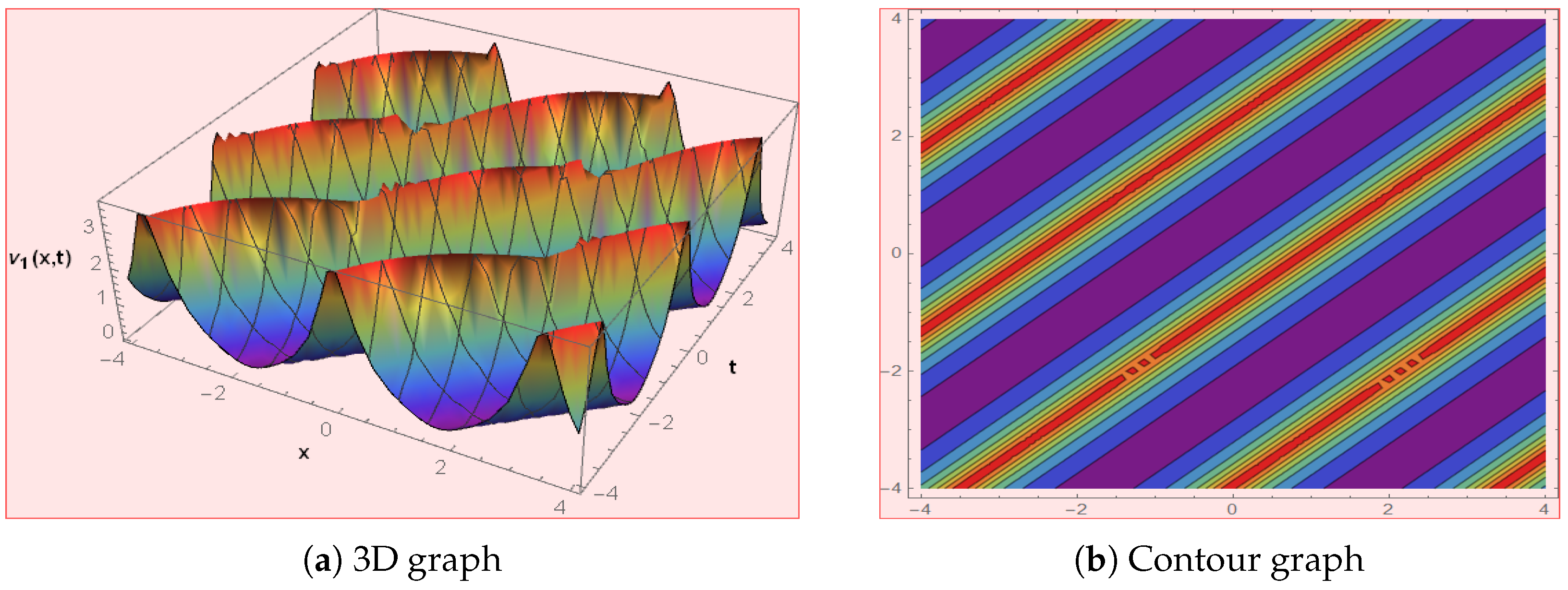
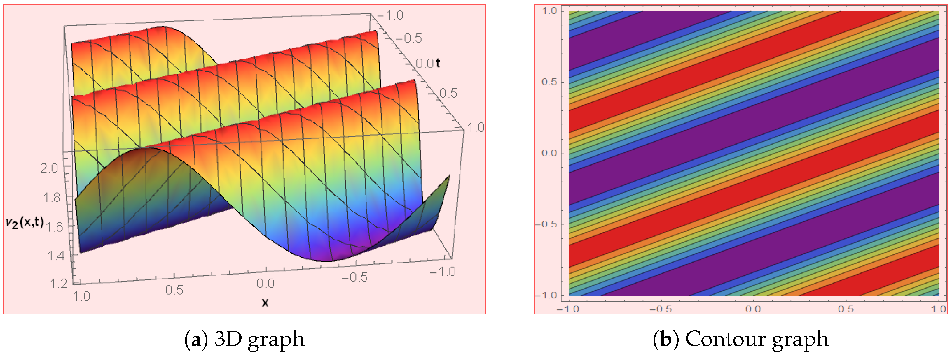
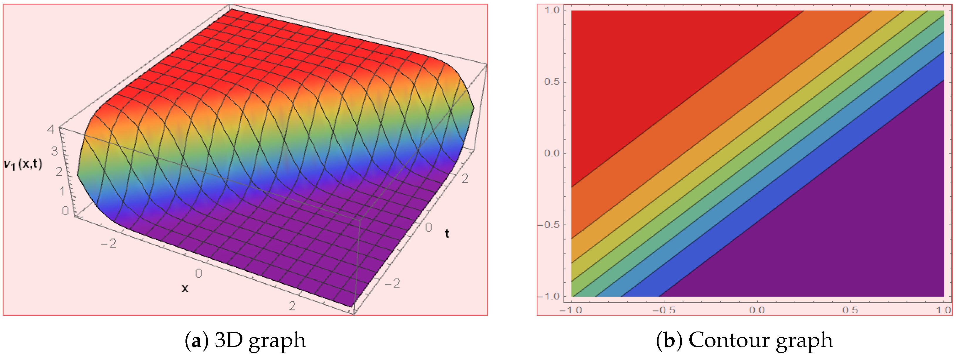
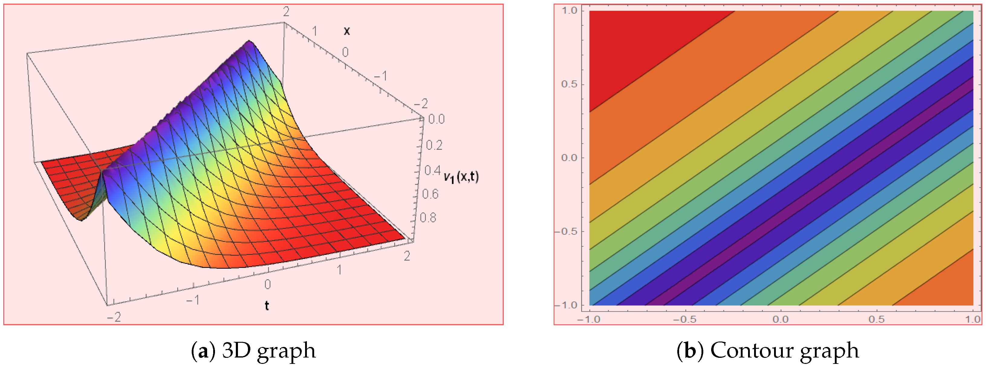
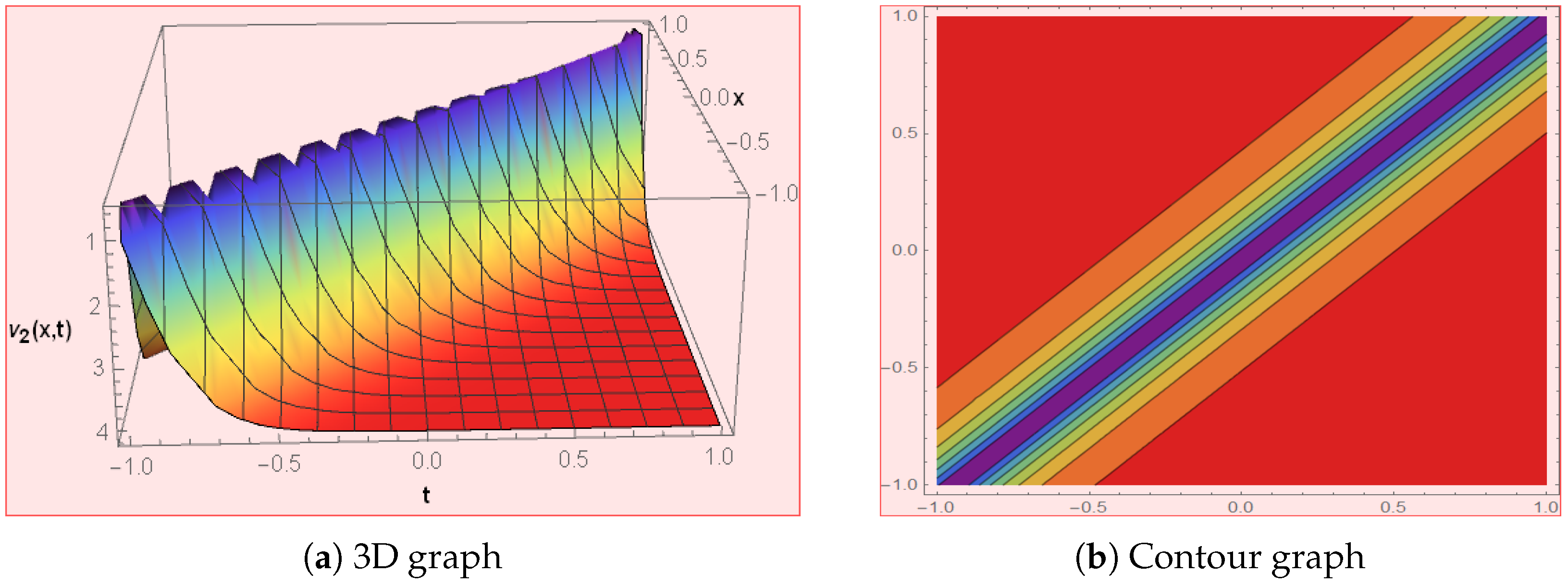
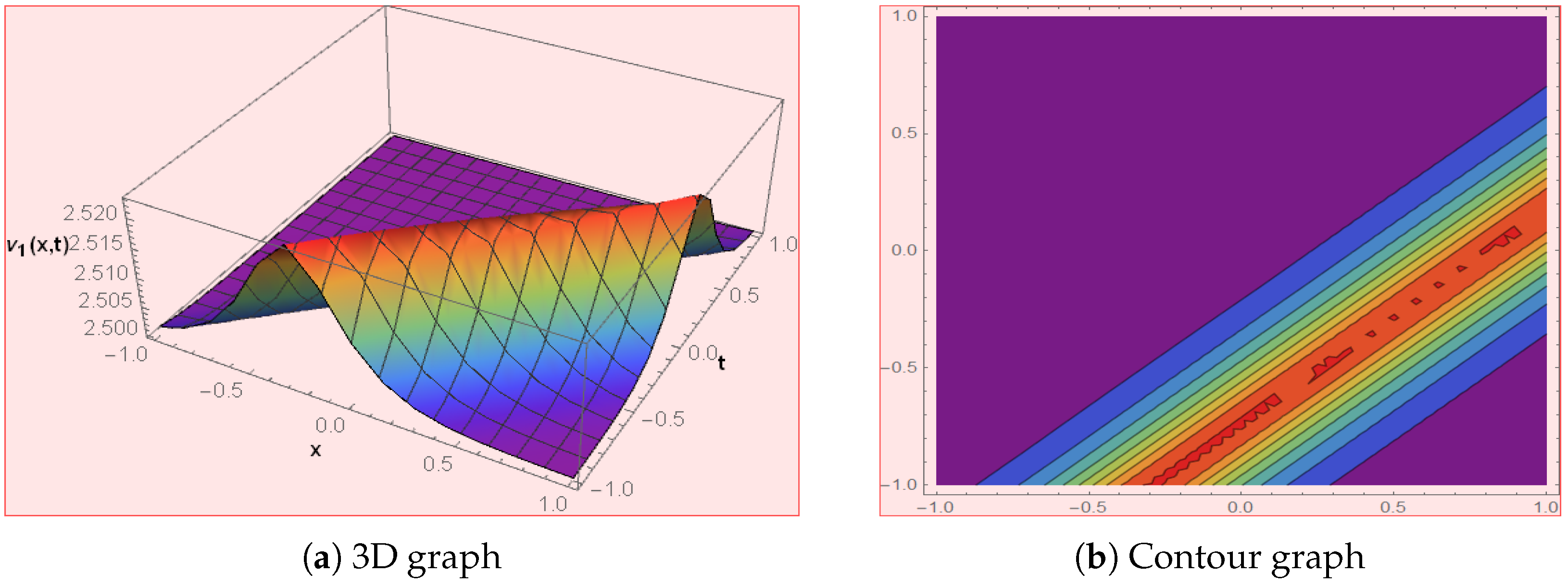
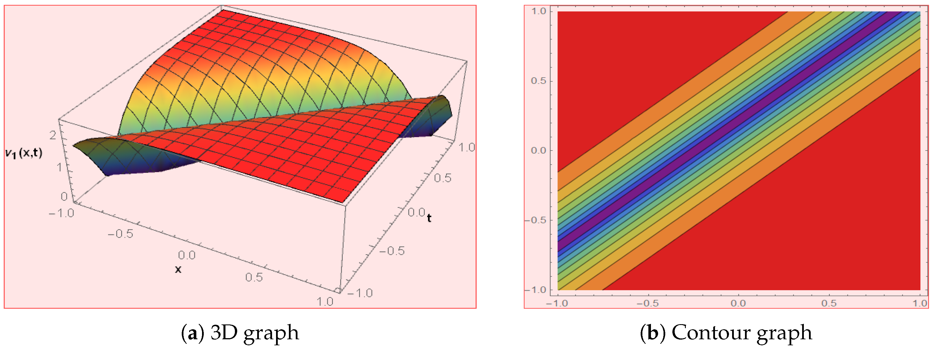
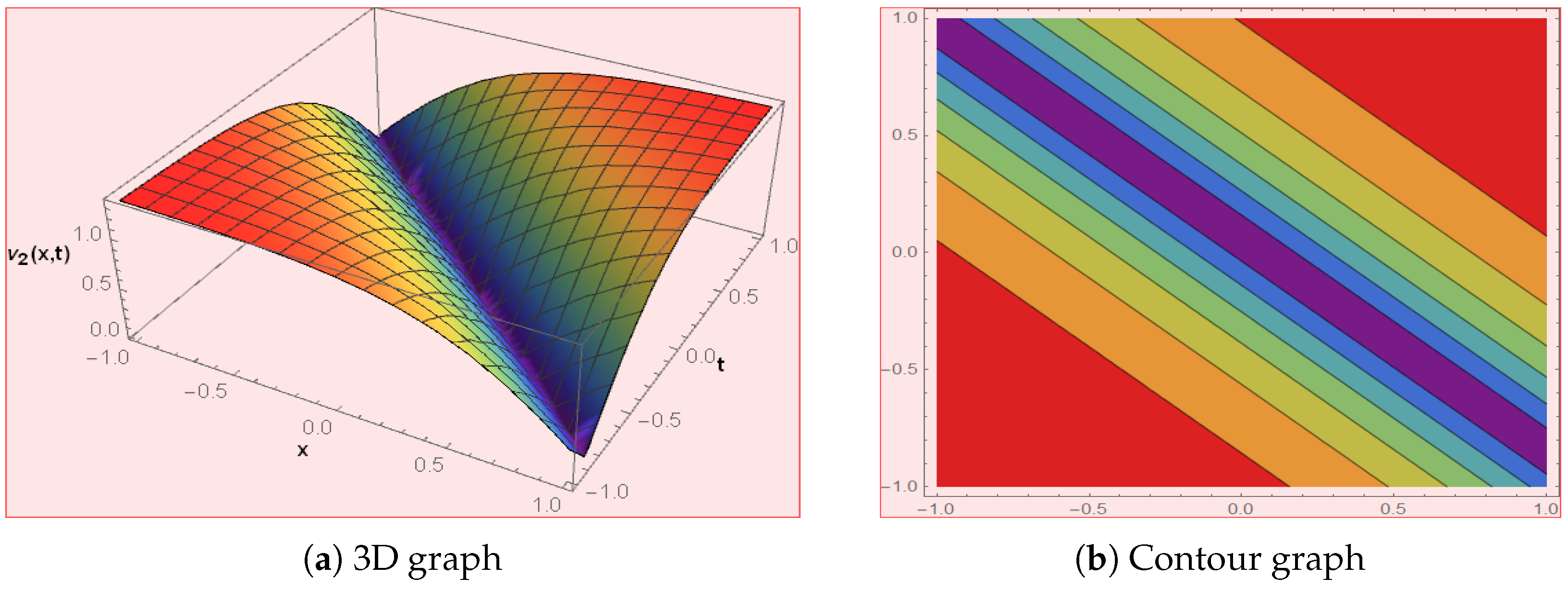
4. Graphical Presentations

Finding soliton solutions was the main goal of this research. Optics is one of the sciences that extensively studies the intriguing physics phenomenon known as a soliton. A self-reinforcing solitary wave is referred to as a soliton if it can keep its shape and speed while moving across a medium without separating or dissipating. Solitons have an unusual behaviour that makes them remarkably stable and enables them to maintain their shape across great distances. These solitons can arise in a variety of waveguide designs, including planar waveguides or ion-acoustic waveguides. Solitons’ capacity to keep their shape and propagate unaltered even in the presence of nonlinear influences and dispersion is their defining feature. Solitons have a physical meaning when they can balance the opposing effects of dispersion and nonlinearity. Over time, dispersion tends to spread out a pulse, causing it to enlarge and change shape. The pulse can be compressed by a self-focusing action brought on by nonlinearity, which, on the other hand, can combat dispersion. For solitons to emerge, nonlinearity and dispersion must coexist in harmony. Ionic-acoustic solitons are created when the nonlinear effects properly balance out the dispersion, creating a localised waveform that is stable and unaltered at vast distances. Solitons are advantageous for numerous applications, including optical signal processing, ultrafast laser pulse propagation, and high-capacity optical communications. Both theoretical and experimental physics have greatly benefited from the discovery and understanding of solitons. They have aided in the growth of uses of ion-acoustic waves and their prospective applications in a variety of fields by providing insights into the interaction between linear and nonlinear effects in wave propagation. Solitons can behave very differently depending on the physical impacts of various dispersion parameters on their dynamics or characteristics.

Dispersion refers to the dependence of the wave’s phase or group velocity on its frequency, and different types of dispersion can arise in different waveguide structures or propagation media. We explored the graphical representations of the aforesaid solutions. The various wave structures below demonstrate graphical depictions of some of the solutions obtained above. Graphs have been extensively utilized to explain the dynamics and distinctive appearance of solutions generated from the BBMPB equation. The results obtained here show that the system has a very diversified wave shape for use in fluid ion applications. Figure 1 and Figure 2 were drawn for the multiwave solutions while Figure 3 shows the kink-type solution for the double rational form solution. Figure 4 and Figure 5 show the breather waves, and Figure 6 corresponds to the mixed-type solution. Figure 7, Figure 8 and Figure 9 represent the physical behaviour of the periodic cross-kink solutions. These solutions are effective in the further study of dynamical systems.

5. Conclusions

The BBMPB model is a useful model for understanding the behaviour of ion-acoustic waves in fluid ions. The ion-acoustic wave is a fundamental mode of oscillation in plasmas and is characterized by its dispersion relation, which relates the wave frequency to the wave number. The study of ion-acoustic waves is of great importance in plasma physics because it provides insights into the basic plasma processes, such as energy transport, wave–particle interactions, and turbulence. The Hirota bilinear transformation technique was used to construct different types of the solutions, and this method gave us the exact ionic wave structures. Different types of wave structures were constructed successfully in the forms of breather waves, lump periodic waves, mixed-type wave solutions, cross-kink rational wave solutions, M-shaped rational wave solutions, and M-shaped rational wave solutions with one or two kink waves. Overall, the study of ion-acoustic wave structures using the BBMPB equation provides valuable insights into the behaviour of plasma waves and the underlying physics of ion-acoustic wave phenomena. The different types of wave solutions studied through this equation gives us a clear understanding of the complex dynamics of these wave structures and may have important implications for the design of plasma-based technologies and experiments.

References

1. Younas, U.; Ren, J.; Baber, M.Z.; Yasin, M.W.; Shahzad, T. Ion-acoustic wave structures in the fluid ions modeled by higher dimensional generalized Korteweg-de Vries–Zakharov–Kuznetsov equation. J. Ocean Eng. Sci. 2022, 7, 1–13. [Google Scholar] [CrossRef]
2. Goswami, A.; Singh, J.; Kumar, D.; Gupta, S. An efficient analytical technique for fractional partial differential equations occurring in ion acoustic waves in plasma. J. Ocean Eng. Sci. 2019, 4, 85–99. [Google Scholar] [CrossRef]
3. Dubinov, A.E. Gas-dynamic approach to the theory of non-linear ion-acoustic waves in plasma with Kaniadakis’ distributed species. Adv. Space Res. 2023, 71, 1108–1115. [Google Scholar] [CrossRef]
4. Usman, M.; Hussain, A.; Zaman, F.D.; Khan, I.; Eldin, S.M. Reciprocal Bäcklund transformations and travelling wave structures of some nonlinear pseudo-parabolic equations. Partial Differ. Equ. Appl. Math. 2023, 7, 100490. [Google Scholar] [CrossRef]
5. Lipatov, A.S. The Hybrid Multiscale Simulation Technology: An Introduction with Application to Astrophysical and Laboratory Plasmas; Springer Science & Business Media: Berlin/Heidelberg, Germany, 2002. [Google Scholar]
6. Xiang, C.; Wang, H. New Exact Solutions for Benjamin-Bona-Mahony-Burgers Equation. Open J. Appl. Sci. 2020, 10, 543–550. [Google Scholar] [CrossRef]
7. Yang, L. Application of classification of traveling wave solutions to the Zakhrov-Kuznetsov-Benjamin-Bona-Mahony equation. Appl. Math. 2014, 5, 1432. [Google Scholar] [CrossRef]
8. Akcagil, S.; Aydemir, T.; Gozukizil, O.F. Exact travelling wave solutions of nonlinear pseudoparabolic equations by using the G G Expansion Method. New Trends Math. Sci. 2016, 4, 51–66. [Google Scholar] [CrossRef]
9. Liu, J.G.; Du, J.Q.; Zeng, Z.F.; Ai, G.P. Exact periodic cross-kink wave solutions for the new (2+1)-dimensional KdV equation in fluid flows and plasma physics. Chaos Interdiscip. J. Nonlinear Sci. 2016, 26, 103114. [Google Scholar] [CrossRef]
10. Song, L.M.; Yang, Z.J.; Li, X.L.; Zhang, S.M. Coherent superposition propagation of Laguerre–Gaussian and Hermite–Gaussian solitons. Appl. Math. Lett. 2020, 102, 106114. [Google Scholar] [CrossRef]
11. Shen, S.; Yang, Z.J.; Pang, Z.G.; Ge, Y.R. The complex-valued astigmatic cosine-Gaussian soliton solution of the nonlocal nonlinear Schrödinger equation and its transmission characteristics. Appl. Math. Lett. 2022, 125, 107755. [Google Scholar] [CrossRef]
12. Shen, S.; Yang, Z.; Li, X.; Zhang, S. Periodic propagation of complex-valued hyperbolic-cosine-Gaussian solitons and breathers with complicated light field structure in strongly nonlocal nonlinear media. Commun. Nonlinear Sci. Numer. Simul. 2021, 103, 106005. [Google Scholar] [CrossRef]
13. Li, X.L.; Guo, R. Interactions of Localized Wave Structures on Periodic Backgrounds for the Coupled Lakshmanan–Porsezian–Daniel Equations in Birefringent Optical Fibers. Ann. Phys. 2023, 535, 2200472. [Google Scholar] [CrossRef]
14. Zou, Z.; Guo, R. The Riemann–Hilbert approach for the higher-order Gerdjikov–Ivanov equation, soliton interactions and position shift. Commun. Nonlinear Sci. Numer. Simul. 2023, 124, 107316. [Google Scholar] [CrossRef]
15. Zhang, S.; Zhu, F.; Xu, B. Localized Symmetric and Asymmetric Solitary Wave Solutions of Fractional Coupled Nonlinear Schrödinger Equations. Symmetry 2023, 15, 1211. [Google Scholar] [CrossRef]
16. Taghizadeh, N.; Mirzazadeh, M. The direct algebraic method to complex nonlinear partial differential equations. Int. J. Appl. Math. Comput. 2013, 5, 12–16. [Google Scholar]
17. Sulaiman, T.A.; Younas, U.; Younis, M.; Ahmad, J.; Rehman, S.U.; Bilal, M.; Yusuf, A. Modulation instability analysis, optical solitons and other solutions to the (2+ 1)-dimensional hyperbolic nonlinear Schrodinger’s equation. Comput. Methods Differ. Equ. 2022, 10, 179–190. [Google Scholar]
18. Seadawy, A.R.; Younis, M.; Baber, M.Z.; Rizvi, S.T.; Iqbal, M.S. Diverse acoustic wave propagation to confirmable time–space fractional KP equation arising in dusty plasma. Commun. Theor. Phys. 2021, 73, 115004. [Google Scholar] [CrossRef]
19. Shahzad, T.; Baber, M.Z.; Ahmad, M.O.; Ahmed, N.; Akgül, A.; Ali, S.M.; Ali, M.; El Din, S.M. On the analytical study of predator–prey model with Holling-II by using the new modified extended direct algebraic technique and its stability analysis. Results Phys. 2023, 51, 106677. [Google Scholar] [CrossRef]
20. Baber, M.Z.; Seadway, A.R.; Iqbal, M.S.; Ahmed, N.; Yasin, M.W.; Ahmed, M.O. Comparative analysis of numerical and newly constructed soliton solutions of stochastic Fisher-type equations in a sufficiently long habitat. Int. J. Mod. Phys. 2023, 37, 2350155. [Google Scholar] [CrossRef]
21. Younas, U.; Sulaiman, T.A.; Ren, J. On the optical soliton structures in the magneto electro-elastic circular rod modeled by nonlinear dynamical longitudinal wave equation. Opt. Quantum Electron. 2022, 54, 688. [Google Scholar] [CrossRef]
22. Feng, Q. A new approach for seeking coefficient function solutions of conformable fractional partial differential equations based on the Jacobi elliptic equation. Chin. J. Phys. 2018, 56, 2817–2828. [Google Scholar] [CrossRef]
23. Hirota, R. The Direct Method in Soliton Theory (No. 155); Cambridge University Press: Cambridge, UK, 2004. [Google Scholar]
24. Ghosh, S.; Bharuthram, R. Ion acoustic solitons and double layers in electron–positron–ion plasmas with dust particulates. Astrophys. Space Sci. 2008, 314, 121–127. [Google Scholar] [CrossRef]
25. Petviashvili, V.I.; Pokhotelov, O.A. Solitary Waves in Plasmas and in the Atmosphere; Taylor & Francis: London, UK, 1992. [Google Scholar]
26. Yuan, W.; Xiao, B.; Wu, Y.; Qi, J. The general traveling wave solutions of the Fisher type equations and some related problems. J. Inequal. Appl. 2014, 2014, 1–15. [Google Scholar] [CrossRef]
27. Wang, X.; Cao, J.; Chen, Y. Higher-order rogue wave solutions of the three-wave resonant interaction equation via the generalized Darboux transformation. Phys. Scr. 2015, 90, 105. [Google Scholar] [CrossRef]
28. Liu, J.G.; Du, J.Q.; Zeng, Z.F.; Nie, B. New three-wave solutions for the (3+1)-dimensional Boiti–Leon–Manna–Pempinelli equation. Nonlinear Dyn. 2017, 88, 655–661. [Google Scholar] [CrossRef]
29. Mihalache, D. Localized structures in optical and matter-wave media: A selection of recent studies. Rom. Rep. Phys. 2021, 73, 403. [Google Scholar]
30. Ma, H.; Zhang, C.; Deng, A. New periodic wave, cross-kink wave, breather, and the interaction phenomenon for the (2+ 1)-dimensional Sharmo–Tasso–Olver equation. Complexity 2020, 2020, 4270906. [Google Scholar] [CrossRef]
31. Alsallami, S.A.; Rizvi, S.T.; Seadawy, A.R. Study of stochastic–fractional Drinfel’d–Sokolov–Wilson equation for M-shaped rational, homoclinic breather, periodic and Kink-Cross rational solutions. Mathematics 2023, 11, 1504. [Google Scholar] [CrossRef]
32. Seadawy, A.R.; Rizvi, S.T.; Younis, M.; Ashraf, M.A. Breather, multi-wave, periodic-cross kink, M-shaped and interactions solutions for perturbed NLSE with quadratic cubic nonlinearity. Opt. Quantum Electron. 2021, 53, 1–14. [Google Scholar] [CrossRef]
Figure 1. The graph depicts the solution of v 1 , 1 ( x , t ) by choosing β = −0.5, c = 1.1, λ = 1.5, n 1 = 1.5, n 2 = 1.5, ϵ 2 = 0.5, and ϵ 4 = 1.5.
Symmetry 15 01682 g001
Figure 2. The graph depicts the solution of v 1 , 2 ( x , t ) by choosing β = 0.5, c = 2.1, λ = 1.5, n 2 = 0.5, n 3 = 0.5, ϵ 4 = 1.5, and ϵ 6 = 2.
Symmetry 15 01682 g002
Figure 3. The graph depicts the solution of v 2 , 1 ( x , t ) by choosing c = 1.01, λ = 1.5, θ = 1.2, n 1 = 0.5, n 2 = 0.5, ϵ 2 = 0.5, and ϵ 4 = 0.5.
Symmetry 15 01682 g003
Figure 4. The graph depicts the solution of v 3 , 1 ( x , t ) by choosing c = 1.1, λ = 0.2, θ = 2.5, n 2 = −1.0, ϵ 2 = 1.5, ϵ 5 = 0.5, and ϵ 6 = 0.1.
Symmetry 15 01682 g004
Figure 5. The graph depicts the solution of v 3 , 2 ( x , t ) by choosing c = 0.985, λ = 1.5, θ = 1.2, n 1 = 1.5, n 2 = 0.67, ϵ 2 = 0.5, ϵ 4 = 1.5, ϵ 5 = 0.9, and ϵ 6 = 0.1.
Symmetry 15 01682 g005
Figure 6. The graph depicts the solution of v 4 , 1 ( x , t ) by choosing c = 1.1, λ = 0.5, θ = 1.2, n 2 = 0.5, n 3 = 0.05, r = 2.1, ϵ 2 = −0.5, and ϵ 4 = −1.5.
Symmetry 15 01682 g006
Figure 7. The graph depicts the solution of v 5 , 1 ( x , t ) by choosing c = 1.1, λ = 0.5, θ = 1.2, n 1 = 1.5, n 3 = 3.5, ϵ 2 = 0.5, ϵ 4 = 1.5, ϵ 7 = 1.5, and ϵ 8 = 1.0.
Symmetry 15 01682 g007
Figure 8. The graph depicts the solution of v 5 , 2 ( x , t ) by choosing c = −1.1, λ = 0.5, θ = 2.2, n 3 = 1.5, ϵ 2 = 0.5, ϵ 7 = 3.5, and ϵ 8 =1.0.
Symmetry 15 01682 g008
Figure 9. The graph depicts the solution of v 5 , 3 ( x , t ) by choosing c = −1.5, λ = 1.5, θ = 2.2, n 3 = 1.5, r = 2.1, ϵ 2 = 0.5, and ϵ 8 =1.0.
Symmetry 15 01682 g009
Disclaimer/Publisher’s Note: The statements, opinions and data contained in all publications are solely those of the individual author(s) and contributor(s) and not of MDPI and/or the editor(s). MDPI and/or the editor(s) disclaim responsibility for any injury to people or property resulting from any ideas, methods, instructions or products referred to in the content.