Further Stability Criteria for Sampled-Data-Based Dynamic Positioning Ships Using Takagi–Sugeno Fuzzy Models

Abstract

This article discusses the stability problem of sampled-data-based dynamic positioning ships (DPSs) using Takagi–Sugeno (T-S) fuzzy models. Firstly, dynamic equations for sampled-data DPSs are established. Simultaneously combining several symmetric matrices with new integral terms, a novel Lyapunov–Krasovskii function (LKF) is constructed, which allows the information of a sampling pattern to be fully captured. Next, via the constructed LKF, the positive definiteness requirements of a LKF are further relaxed, and the conservatism of the result can be reduced. Consequently, stability criteria are given, and fuzzy sampled-data controllers are designed in terms of linear matrix inequality (LMI). Finally, a simulation example is provided to verify the superiority and applicability of the developed methods.

1. Introduction

A DPS is a system that utilizes a combination of computers, position reference systems, and thrusters to maintain a ship at a predetermined position [1]. It uses the measurement equipment of the ship to collect environmental parameters, calculates the thrust of the thruster based on the parameters of the global positioning system, and maintains fixed positions and headings. Compared with anchoring positioning, a DPS relies only on ship thrusters to overcome environmental interference and achieves the desired position for engineering operations. Therefore, it has unique advantages, such as infinite depth operation, high mobility, and precise positioning. And a DPS has a wide range of applications, such as cargo supply, oil extraction, heavy lifting, ocean surveying, deep water exploration, ocean rescue, etc. Therefore, more and more scholars are studying the control problem of DPSs ([2,3,4,5,6,7]). For example, reference [2] conducted fuzzy modeling for a DPS based on the range of the yaw angle, and designed an observer that can provide excellent DP performances that reduces the negative impact of external disturbance. Reference [3] designed a quantization controller based on a switching mechanism to ensure the robustness and control performance of a DPS, and signal quantization, time delay, and thruster failure were simultaneously considered. Reference [4] used a neural network to design a system controller for a DPS, and auxiliary devices like thruster and tug were considered. Reference [5] proposed a multitask control system for a DPS by introducing the integrated neural controller, and the neural network structures were not required to be retrained while performing different tasks. Reference [6] combined Luenberger observer and odd–even space technology to DPS detect thruster faults, and designed a reconfigurable variable structure controller to achieve fault-tolerant targets.

Recently, digital devices have been gradually replacing continuous time devices in actual industrial systems. These control systems, which include continuous time objects and discrete time controllers, are considered sampled-data control systems. Compared with traditional continuous time control systems, sampled-data control systems only require the instantaneous sampling information of the system state, and thus greatly reduce information transmission and communication costs. Therefore, they are widely applicable in various systems, such as multiagent systems [8,9], chaotic systems [10,11], master–slave systems [12], neural networks systems [13,14], Markovian jump systems [15], time delay systems [16,17], etc. They have also been used in severable practical engineering applications, including high-speed trains [18], autonomous airships [19], multipurpose supply vessels [20], luxury cruises [21], unmanned marine vehicles [22], etc. For example, reference [23] studied a discrete sampled-data system with a saturated actuator, and designed a robust controller using a convex approach to ensure the local stability of the systems with interval time delays. Reference [24] creatively introduced an algorithm for event-triggered sampling control and proposed intermittent triggering conditions at fixed sampling times. Reference [25] focused on a class of multi-agent systems and transformed them into discrete systems, analyzed the inherent relationship between the sampling period and steady-state performance, and obtained the range of the sampling period. Reference [26] investigated the mean square exponential stability problem of a sampled-data resistive memory neural network (MNN) system. The concept of security level was first proposed to measure the anti-attack capability of a MNN. Reference [27] proposed a dual deep Q-network method to solve the sampled-data control problem of PBCNs, and an optimal sampled-data controller was designed to stabilize the PBCN.

Nowadays, T-S fuzzy systems (TSFSs) have obtained wide attention [28], and severable sampled-data control results have been reported for TSFSs. Reference [29] investigated the adaptive static output control problem of TSFSs with uncertainties. To reduce the sampled-data frequency, new adaptive memory event-triggering mechanisms were proposed. Reference [30] investigated the quantitative sampled-data control issue of a network TSFS using a random network attack, and then new time delay product relaxation conditions were proposed. Reference [31] proposed a non-periodic event-triggered communication scheme to solve the exponential stabilization issue of TSFSs under non-periodic sampling conditions. Reference [32] investigated the stability problem of TSFSs under sampled-data control using a new asymmetric LKF. Cyclic and discontinuous function terms were improved by combining time delay and each sampling interval. Reference [33] investigated the stability characteristics of a TSFS under sampled-data control. Based on the input delay method, the system was converted to a variable time-delay system. Using the reciprocally convex combination approach, stability criteria were established to guarantee the stability of the TSFS.

A DPS is a sampled-data control system that uses a computer to collect severable sensor information, and then the sailing status of the ship is obtained [34]. Recently, many sampled-data control achievements of DPSs have been reported. In [35], the trajectory tracking problem of a nonlinear sampled-data DPS was considered, and a reduced order observer was introduced using the Euler approximation model. In [36], the systems of the sampled-data DPS were converted into neutral systems; then the Wirtinger integral inequality and delay-decomposition methods were introduced to reduce the conservatism of the system. In [37], the fault-tolerant control problem of a sampled-data DPS was studied using actuator failure. Reference [38] established fuzzy models for a sampled-data DPS, and convex reciprocal inequalities were used to obtain the stability condition. Reference [39] investigated the non-periodic sampling tracking control problem of a DPS using actuator faults, and by introducing a new LKF, the mean square exponential stability criterion was obtained.

However, there is still room for improvement regarding the sampling control problem of DPSs. Firstly, during the LKF construction process, some terms in a LKF share common quadratic functions. Secondly, some available information for sampling patterns is completely ignored. Thirdly, conditions on LKFs are too strict; that is, some matrices in a single Lyapunov are strictly positive definite. To some extent, these limitations lead to a decrease in the conservatism of the results.

Motivated by the above analysis, the fuzzy sampling control problem of a nonlinear DPS is studied here. Firstly, the dynamic equations of the system are established. Secondly, an improved LKF is established to fully capture the characteristics of sampling modes and further relax the positive definiteness requirements of LKFs. Based on the LMIs, stability conditions are derived, and the designed approach of the sampling controller is given. Finally, the superiority of this method is verified through a simulation example.

The developments and novelty of this article are summarized as follows.

(1) By introducing some novel terms, like $d(t){\displaystyle {\int }_{-d(t)}^0{\displaystyle {\int }_{t+\theta }^t\dot{x}{(s)}^{T}Z\dot{x}(s)dsd\theta }}$, in the LKF, the available characteristics of sampling patterns have been fully captured.

(2) Compared with the LKF in existing results, more available matrices are effectively used in the LKF. Therefore, the proposed LKF has a more general form.

(3) Compared with the existing results, X-dependent terms are introduced in the LKF, which are not required to be positive definite, and this means that the limitation conditions of the symmetric matrices are overcome.

Notations: ${ℝ}^m$ is m-dimensional Euclidean space, $M^T$ is the transpose of matrix $M$, “*” is the symmetric term of a matrix, and $‖·‖$ is the spectral norm in ${ℝ}^m$.

The subsequent structure of this article is as follows. In Section 2, models of the sampled-data DPS system are established. In Section 3, the main results are described. In Section 4, numerical validation and comparison results are described.

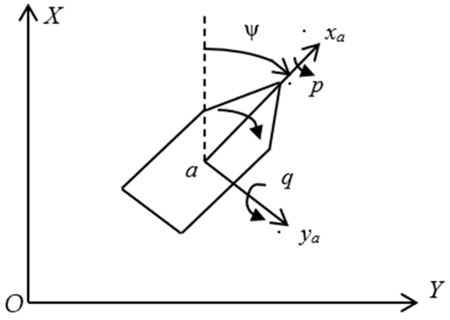
2. Problem Formulation

In order to deal with the sampled-data control problem for DPSs, dynamic equations for a DPS are considered:

$$\begin{array}{l}M\dot{\upsilon }(t)+D\upsilon (t)+G\eta (t)=u(t),\\ \dot{\eta }(t)=J\left(\psi (t)\right)\upsilon (t),\end{array}$$

(1)

where

$$\begin{array}{l}M=\left[\begin{array}{ccc}m-X_{\dot{u}}& 0& 0\\ 0& m-Y_{\dot{v}}& m{x}_G-Y_{\dot{r}}\\ 0& m{x}_G-Y_{\dot{r}}& I_z-N_{\dot{r}}\end{array}\right],D=\left[\begin{array}{ccc}-X_{\dot{u}}& 0& 0\\ 0& -Y_{\dot{v}}& -Y_{\dot{r}}\\ 0& -Y_{\dot{r}}& -N_{\dot{r}}\end{array}\right],\\ J\left(\psi (t)\right)=\left[\begin{array}{ccc}\cos \left(\psi (t)\right)& -\sin \left(\psi (t)\right)& 0\\ \sin \left(\psi (t)\right)& \cos \left(\psi (t)\right)& 0\\ 0& 0& 1\end{array}\right].\end{array}$$

where $\eta (t)={\left[\begin{array}{ccc}{x}_a(t)& y_a(t)& \psi (t)\end{array}\right]}^T$ is the position vector in the northeast coordinate system; $x_a(t)$ and $y_a(t)$ represent the x and y positions, respectively; and $\psi (t)$ represents the yaw angle. $\upsilon (t)={\left[\begin{array}{ccc}p(t)& v(t)& r(t)\end{array}\right]}^T$ denotes the velocity vector in the attached coordinate system (see Figure 1). $p(t)$ is surge velocity; $v(t)$ is sway velocity; and $r(t)$ is yaw velocity. $J\left(\psi \right)$ represents the rotation matrix of the two coordinates. $u(t)$ is the control force vector; and $M$ and $D$ are the inertial matrix and damping matrix, respectively. $G=diag\left\{g_{11},g_{22},g_{33}\right\}$ represents the mooring force matrix. $m$ is the ship’s mass; $I_z$ is the moment of inertia; $x_G$ is the distance vector; and $X_{\dot{u}}$, $Y_{\dot{v}}$, $N_{\dot{r}}$ $Y_{\dot{r}}$ are the added mass.

Remark 1.

The derivation of the ship model is based on [1]. The case study in this paper is a dynamic positioning ship controlled by thrusters. The damping force is assumed to be linear because the ship’s speed is slow. Therefore, dynamic equations for surge, sway, and yaw for the DPS are considered in this paper.

Define

$$\begin{array}{ll}x(t)& ={\left[\begin{array}{cc}\eta (t)& \upsilon (t)\end{array}\right]}^T\\ & ={\left[\begin{array}{cccccc}{x}_a(t)& y_a(t)& \psi (t)& p(t)& q(t)& r(t)\end{array}\right]}^T,\end{array}$$

(2)

and let

$$-M^{-1}D=\left[\begin{array}{ccc}{a}_{11}& 0& 0\\ 0& a_{22}& a_{23}\\ 0& a_{32}& a_{33}\end{array}\right],M^{-1}=\left[\begin{array}{ccc}{d}_{11}& 0& 0\\ 0& d_{22}& d_{23}\\ 0& d_{32}& d_{33}\end{array}\right],-M^{-1}G=\left[\begin{array}{ccc}{b}_{11}& 0& 0\\ 0& b_{22}& b_{23}\\ 0& b_{32}& b_{33}\end{array}\right].$$

(3)

where $a_{11},a_{22},a_{23},a_{32},a_{33},d_{11},d_{22},d_{23},d_{32},d_{33},b_{11},b_{22},b_{23},b_{32},b_{33}$ are constant.

Substitute (2) and (3) into (1) that

$$\dot{x}(t)=A(t)x(t)+Bu(t),$$

(4)

where

$$A(t)=\left[\begin{array}{cccccc}0& 0& 0& \cos \left(\psi (t)\right)& -\sin \left(\psi (t)\right)& 0\\ 0& 0& 0& \sin \left(\psi (t)\right)& \cos \left(\psi (t)\right)& 0\\ 0& 0& 0& 0& 0& 1\\ b_{11}& 0& 0& a_{11}& 0& 0\\ 0& b_{22}& b_{23}& 0& a_{22}& a_{23}\\ 0& b_{32}& b_{33}& 0& a_{32}& a_{33}\end{array}\right],B=\left[\begin{array}{ccc}0& 0& 0\\ 0& 0& 0\\ 0& 0& 0\\ d_{11}& 0& 0\\ 0& d_{22}& d_{23}\\ 0& d_{32}& d_{33}\end{array}\right].$$

The overall fuzzy model is obtained that

Mode Rule i: IF $z_1(t)$ is $f_{\mathrm{i}1}$, $\cdots z_n(t)$ is $f_{\mathrm{in}}$, THEN

$$\dot{x}(t)=A_{i}x(t)+B_{i}u(t),i=1,2,\dots ,n$$

(5)

where $z_1(t),z_2(t),\dots ,z_{\mathrm{n}}(t)$ denote premise variables, $f_{\mathrm{ij}}$ denotes the fuzzy set, and n denotes the rules number.

Assume the yaw angle satisfies $\psi (t)\in \left(-\pi /2,\pi /2\right)$, then T-S fuzzy rules are considered that

Model Rule 1:

IF $\psi (t)$ is about 0

Then

$$\dot{x}(t)=A_{1}x(t)+B_{1}u(t),$$

(6)

Model Rule 2:

IF $\psi (t)$ is about $\frac{\pi }{2}$$\left(\psi \left(t\right)<\frac{\pi }{2}\right)$

Then

$$\dot{x}(t)=A_{2}x(t)+B_{2}u(t),$$

(7)

Model Rule 3:

IF $\psi (t)$ is about $-\frac{\pi }{2}$$\left(\psi \left(t\right)<\frac{\pi }{2}\right)$

Then

$$\dot{x}(t)=A_{3}x(t)+B_{3}u(t),$$

(8)

where

$$\begin{array}{l}{A}_1=\left[\begin{array}{cccccc}0& 0& 0& 1& -\alpha & 0\\ 0& 0& 0& \alpha & 1& 0\\ 0& 0& 0& 0& 0& 1\\ b_{11}& 0& 0& a_{11}& 0& 0\\ 0& b_{22}& b_{23}& 0& a_{22}& a_{23}\\ 0& b_{32}& b_{33}& 0& a_{32}& a_{33}\end{array}\right],A_2=\left[\begin{array}{cccccc}0& 0& 0& \beta & -1& 0\\ 0& 0& 0& 1& \beta & 0\\ 0& 0& 0& 0& 0& 1\\ b_{11}& 0& 0& a_{11}& 0& 0\\ 0& b_{22}& b_{23}& 0& a_{22}& a_{23}\\ 0& b_{32}& b_{33}& 0& a_{32}& a_{33}\end{array}\right],\\ A_3=\left[\begin{array}{cccccc}0& 0& 0& \beta & 1& 0\\ 0& 0& 0& -1& \beta & 0\\ 0& 0& 0& 0& 0& 1\\ b_{11}& 0& 0& a_{11}& 0& 0\\ 0& b_{22}& b_{23}& 0& a_{22}& a_{23}\\ 0& b_{32}& b_{33}& 0& a_{32}& a_{33}\end{array}\right],B_i=\left[\begin{array}{ccc}0& 0& 0\\ 0& 0& 0\\ 0& 0& 0\\ d_{11}& 0& 0\\ 0& d_{22}& d_{23}\\ 0& d_{32}& d_{33}\end{array}\right],i=1,2,3.\end{array}$$

and in which $\alpha =\sin \left(2^{\circ }\right)$ and $\beta =\cos \left({88}^{\circ }\right)$. The overall T-S fuzzy model is obtained that

$$\dot{x}(t)={\displaystyle \sum _{i=1}^3{\mu }_i(z(t))\left[A_{i}x(t)+B_{i}u(t)\right]},$$

(9)

where

$$\begin{array}{l}{\mu }_i(z(t))=\frac{{\omega }_i(z(t))}{{\displaystyle \sum _{i=1}^3{\omega }_i(z(t))}}\ge 0,i=1,2,3,\\ {\omega }_i(z(t))={\displaystyle \prod _{j=1}^n{f}_{ij}(z_j(t))},\\ {\displaystyle \sum _{i=1}^3{\mu }_i(z(t))}=1,\\ z(t)=\left[z_1(t),z_2(t),\dots ,z_n(t)\right],\end{array}$$

and in which $f_{ij}(z_j(t))$ denotes the membership grade of $z_j(t)$. The membership function of $\psi (t)$ is shown in Figure 2.

A diagram of the fuzzy modeling and controller design is shown in Figure 3.

Assume measurement signals of the DPS are available at the sampling time, which satisfies that $0=t_0<t_1<\cdots <t_k<\cdots <\underset{k\to \infty }{\lim }{t}_k=+\infty$.

The sampling interval is supposed as

$$t_{k+1}-t_k\le d,\forall k\ge 0,d>0,$$

where $d$ denotes the upper bound of the sampling interval. Next, the corresponding sampled-data controller is considered

$$u(t)=Kx(t_k),t_k\le t<t_{k+1},$$

(10)

where $K$ denotes the gain matrix. Next, T-S fuzzy controllers are expressed that

Controller Rule 1:

IF $\psi (t)$ is about 0

Then

$$u(t)=K_{1}x(t_k).$$

(11)

Controller Rule 2:

IF $\psi (t)$ is about $\frac{\pi }{2}$$\left(\psi \left(t\right)<\frac{\pi }{2}\right)$

Then

$$u(t)=K_{2}x(t_k).$$

(12)

Controller Rule 3:

IF $\psi (t)$ is about $-\frac{\pi }{2}$$\left(\psi \left(t\right)<\frac{\pi }{2}\right)$

Then

$$u(t)=K_{3}x(t_k).$$

(13)

Next, the following fuzzy controller is obtained

$$u(t)={\displaystyle \sum _{j=1}^3{\mu }_j(z(t))K_{j}x(t_k)},t_k\le t<t_{k+1},k=0,1,2,\dots$$

(14)

Substitute (14) into (11) to obtain

$$\dot{x}(t)={\displaystyle \sum _{i=1}^3{\displaystyle \sum _{j=1}^3{\mu }_i(z(t)){\mu }_j(z(t))\left[A_{i}x(t)+B_i{K}_{j}x(t_k)\right]}}$$

(15)

For the further deriving process, the lemma is given as:

Lemma 1

([40]). For given matrix $Z\in {ℝ}^n,Z>0$, scalars ${\tau }_2>{\tau }_1$, vector function $w:\left[{\tau }_1,{\tau }_2\right]\in R^n$, the following inequality holds

$$\begin{array}{l}-{\displaystyle {\int }_{t-{\tau }_2}^{t-{\tau }_1}{w}^T(\alpha )Zw(\alpha )d\alpha }\\ \le -\frac{1}{{\tau }_2-{\tau }_1}{\left({\displaystyle {\int }_{t-{\tau }_2}^{t-{\tau }_1}{w}^T(\alpha )d\alpha }\right)}^{T}Z\left({\displaystyle {\int }_{t-{\tau }_2}^{t-{\tau }_1}w(\alpha )d\alpha }\right)\end{array}$$

(16)

$$\begin{array}{l}-{\displaystyle {\int }_{-{\tau }_2}^{-{\tau }_1}{\displaystyle {\int }_{t+\alpha }^t{w}^T(s)Zw(s)dsd\alpha }}\\ \le -\frac{2}{{\tau }_2^2-{\tau }_1^2}{\left({\displaystyle {\int }_{-{\tau }_2}^{-{\tau }_1}{\displaystyle {\int }_{t+\alpha }^t{w}^T(s)dsd\alpha }}\right)}^{T}Z\left({\displaystyle {\int }_{-{\tau }_2}^{-{\tau }_1}{\displaystyle {\int }_{t+\alpha }^{t}w(s)dsd\alpha }}\right)\end{array}$$

(17)

3. Main Results

In this section, by constructing an appropriate LKF, the stability conditions of system (15) are given.

3.1. Construction of the Lyapunov Function

Firstly, the notations are defined as follows:

$$\begin{array}{l}\tau (t)=t-t_k,d(t)=d-\tau (t),\\ \varsigma (t)={\left[\begin{array}{ccc}{x}^T(t)& x^T(t_k)& {\displaystyle {\int }_{t_k}^t{x}^T(s)ds}\end{array}\right]}^T\\ \zeta (t)=\left[\begin{array}{cccc}{x}^T(t)& \dot{x}{(t)}^T& x^T(t_k)& {\displaystyle {\int }_{t_k}^t{x}^T(s)ds}\end{array}\right]\end{array}$$

Theorem 1.

The system (15) is asymptotically stable, if there exist symmetric matrices$P>0,Q>0,Z>0,\left[\begin{array}{cc}{R}_{11}& R_{12}\\ \ast & R_{22}\end{array}\right]>0,\left[\begin{array}{cc}{U}_{11}& U_{12}\\ \ast & U_{22}\end{array}\right]>0,X_{11},X_{13},X_{22},X_{23},X_{33},G,$ $M_{ij}={\left[\begin{array}{cccc}{M}_{1ij}^T& M_{2ij}^T& M_{3ij}^T& M_{4ij}^T\end{array}\right]}^T,N_{ij}={\left[\begin{array}{cccc}{N}_{1ij}^T& N_{2ij}^T& N_{3ij}^T& N_{4ij}^T\end{array}\right]}^T$and scales $d>0$,${\epsilon }_i,i=1,2,3,4$, such that

$${\mathsf{\Psi }}_1^{ij}=\left[\begin{array}{ccc}P+d\left(X_{11}+X_{11}^T+Q\right)& d\left(X_{11}+X_{22}-Q\right)& d{X}_{13}\\ \ast & d\left(X_{11}+X_{22}^T+Q\right)& d{X}_{23}\\ \ast & \ast & d{X}_{33}\end{array}\right]>0$$

(18)

$${\mathsf{\Psi }}_2^{ij}=\left[\begin{array}{cccc}{\mathsf{\Xi }}_{11}^{ij}+{\mathsf{\Omega }}_{11}^{ij}& {\mathsf{\Xi }}_{12}^{ij}+{\mathsf{\Omega }}_{12}^{ij}& {\mathsf{\Xi }}_{13}^{ij}+{\mathsf{\Omega }}_{13}^{ij}& {\mathsf{\Xi }}_{14}^{ij}+d{X}_{33}^T\\ \ast & {\mathsf{\Xi }}_{22}^{ij}+{\mathsf{\Omega }}_{22}^{ij}& {\mathsf{\Xi }}_{23}^{ij}+{\mathsf{\Omega }}_{23}^{ij}& {\mathsf{\Xi }}_{11}^{ij}+d{X}_{13}\\ \ast & \ast & {\mathsf{\Xi }}_{33}^{ij}+{\mathsf{\Omega }}_{33}^{ij}& {\mathsf{\Xi }}_{34}^{ij}\\ \ast & \ast & \ast & {\mathsf{\Xi }}_{44}^{ij}\end{array}\right]<0$$

(19)

$${\mathsf{\Psi }}_3^{ij}==\left[\begin{array}{cc}{\mathsf{\Pi }}_{11ij}& {\mathsf{\Pi }}_{12ij}\\ \ast & {\mathsf{\Pi }}_{22}\end{array}\right]<0.$$

(20)

where

$$\begin{array}{l}{\mathsf{\Pi }}_{11ij}=\left[\begin{array}{cccc}{\mathsf{\Xi }}_{11}^{ij}+{\mathsf{\Omega }}_{11}^{ij}& {\mathsf{\Xi }}_{12}^{ij}+d{N}_{2ij}^T& {\mathsf{\Xi }}_{13}^{ij}+d{N}_{3ij}^T& {\mathsf{\Xi }}_{14}^{ij}+d{N}_{4ij}^T\\ \ast & {\mathsf{\Xi }}_{22}^{ij}+\frac{d^2}{4}Z& {\mathsf{\Xi }}_{23}^{ij}& {\mathsf{\Xi }}_{24}^{ij}\\ \ast & \ast & {\mathsf{\Xi }}_{33}^{ij}+{\mathsf{\Omega }}_{33}^{ij}& {\mathsf{\Xi }}_{34}^{ij}\\ \ast & \ast & \ast & {\mathsf{\Xi }}_{44}^{ij}\end{array}\right],\\ {\mathsf{\Pi }}_{12ij}=\left[\begin{array}{cc}-d{M}_{1ij}& d{N}_{1ij}\\ -d{M}_{2ij}& d{N}_{2ij}\\ -d{E}^T{R}_{12}^T-d{M}_{3ij}& d{N}_{3ij}\\ -d{M}_{4ij}& d{N}_{4ij}\end{array}\right],\\ {\mathsf{\Pi }}_{22}=\left[\begin{array}{cc}-dQ-d{R}_{11}& 0\\ \ast & -2Z\end{array}\right],\\ {\mathsf{\Xi }}_{11}^{ij}=-\left(X_{11}+X_{11}^T\right)+M_{1ij}^T+M_{1ij}+{\epsilon }_1{A}_i{G}^T+{\epsilon }_{1}G{A}_i^T\\ {\mathsf{\Xi }}_{12}^{ij}=P+M_{2ij}^T-{\epsilon }_{1}G-{\epsilon }_2{A}_i^T{G}^T\\ {\mathsf{\Xi }}_{13}^{ij}=\left(X_{11}+X_{22}\right)+M_{3ij}^T-M_{1ij}+{\epsilon }_{1}G{B}_i{K}_j+{\epsilon }_3{A}_i^T{G}^T\\ {\mathsf{\Xi }}_{14}^{ij}=-X_{13}+M_{4ij}^T-N_{1ij}+{\epsilon }_4{A}_i^T{G}^T\\ {\mathsf{\Xi }}_{22}^{ij}=-{\epsilon }_{2}G-{\epsilon }_2{G}^T\\ {\mathsf{\Xi }}_{23}^{ij}=-M_{2ij}+{\epsilon }_{2}G{B}_i{K}_j-{\epsilon }_3{G}^T\\ {\mathsf{\Xi }}_{24}^{ij}=-{\epsilon }_4{G}^T-N_{2ij}\\ {\mathsf{\Xi }}_{33}^{ij}=-\left(X_{22}+X_{22}^T\right)-M_{3ij}^T-M_{3ij}+{\epsilon }_{3}G{B}_i{K}_j+{\epsilon }_3{K}_j^T{B}_i^T{G}^T\\ {\mathsf{\Xi }}_{34}^{ij}=-X_{23}-U_{12}-M_{4ij}^T-N_{3ij}+{\epsilon }_4{K}_j^T{B}_i^T{G}^T\\ {\mathsf{\Xi }}_{44}^{ij}=-X_{33}-\frac{1}{d}{U}_{22}-N_{4ij}^T-N_{4ij}\\ {\mathsf{\Omega }}_{11}=d\left(X_{13}+X_{13}^T\right)+d{U}_{22}-Z\\ {\mathsf{\Omega }}_{12}=d{X}_{11}+d{X}_{11}^T\\ {\mathsf{\Omega }}_{13}=d{X}_{23}^T+d{U}_{12}^T+Z\\ {\mathsf{\Omega }}_{22}=d{R}_{11}+dQ+\frac{d^2}{4}Z\\ {\mathsf{\Omega }}_{23}=-d\left(X_{11}+X_{22}\right)+d{R}_{12}\\ {\mathsf{\Omega }}_{33}=d{R}_{22}+d{U}_{11}-Z\\ \end{array}$$

Proof. 

Consider the following LKF

$$V(t)={\displaystyle \sum _{i=1}^4{V}_i(t),t\in [t_k,t_{k+1})}$$

(21)

$$\begin{array}{l}{V}_1(t)=x{(t)}^{T}Px(t)+d(t)\varsigma {(t)}^{T}X\varsigma (t)+d(t){\displaystyle {\int }_{t_k}^t\dot{x}{(s)}^{T}Q\dot{x}(s)ds}\\ V_2(t)=d(t){\displaystyle {\int }_{t_k}^t{\left[\begin{array}{c}\dot{x}(s)\\ x(t_k)\end{array}\right]}^{T}R\left[\begin{array}{c}\dot{x}(s)\\ x(t_k)\end{array}\right]ds}\\ V_3(t)=d(t){\displaystyle {\int }_{t_k}^t{\left[\begin{array}{c}x(t_k)\\ x(s)\end{array}\right]}^{T}U\left[\begin{array}{c}x(t_k)\\ x(s)\end{array}\right]ds}\\ V_4(t)=d(t){\displaystyle {\int }_{-d(t)}^0{\displaystyle {\int }_{t+\theta }^t\dot{x}{(s)}^{T}Z\dot{x}(s)dsd\theta }}\end{array}$$

where

$$\begin{array}{l}X=\left[\begin{array}{ccc}{X}_{11}+X_{11}^T& -X_{11}-X_{22}& X_{13}\\ \ast & X_{22}+X_{22}^T& X_{23}\\ \ast & \ast & X_{33}\end{array}\right],\\ R=\left[\begin{array}{cc}{R}_{11}& R_{12}\\ \ast & R_{22}\end{array}\right],U=\left[\begin{array}{cc}{U}_{11}& U_{12}\\ \ast & U_{22}\end{array}\right]\end{array}$$

Using Lemma 1, the following inequality is obtained:

$$\begin{array}{ll}{V}_1(t)& \ge x{(t)}^{T}Px(t)+d(t)\varsigma {(t)}^{T}X\varsigma (t)+\frac{d(t)}{d}{\left[x(t)-x(t_k)\right]}^{T}Q\left[x(t)-x(t_k)\right]\\ & =\frac{d(t)}{d}{\varsigma }^T(t){\mathsf{\Psi }}_1^{ij}\varsigma (t)\end{array}$$

(22)

From LMI (18), $V_1(t)\ge 0$ can be guaranteed, which means that $V(t)\ge 0$.

Taking the derivative of $V(t)$ yields

$$\begin{array}{ll}{\dot{V}}_1(t)& =2\dot{x}{(t)}^{T}Px(t)+2d(t){\varsigma }^T(t)X{\left[\begin{array}{ccc}{\dot{x}}^T(t)& 0& x^T(t)\end{array}\right]}^T\\ & -{\varsigma }^T(t)X\varsigma (t)+d(t){\dot{x}}^T(t)Q\dot{x}(t)-{\displaystyle {\int }_{t_k}^t{\dot{x}}^T(s)Q\dot{x}(s)ds},\\ {\dot{V}}_2(t)& =d(t){\left[\begin{array}{c}\dot{x}(t)\\ x(t_k)\end{array}\right]}^{T}R\left[\begin{array}{c}\dot{x}(t)\\ x(t_k)\end{array}\right]-{\displaystyle {\int }_k^t{\left[\begin{array}{c}\dot{x}(s)\\ x(t_k)\end{array}\right]}^{T}R\left[\begin{array}{c}\dot{x}(s)\\ x(t_k)\end{array}\right]ds,}\\ {\dot{V}}_3(t)& =d(t){\left[\begin{array}{c}x(t_k)\\ x(t)\end{array}\right]}^{T}U\left[\begin{array}{c}x(t_k)\\ x(t)\end{array}\right]-{\displaystyle {\int }_{t_k}^t{\left[\begin{array}{c}x(t_k)\\ x(s)\end{array}\right]}^{T}U\left[\begin{array}{c}x(t_k)\\ x(s)\end{array}\right]ds}\\ & =d(t){\left[\begin{array}{c}x(t_k)\\ x(t)\end{array}\right]}^{T}U\left[\begin{array}{c}x(t_k)\\ x(t)\end{array}\right]-\tau (t)x^T(t_k)U_{11}x(t_k)\\ & =-2x^T(t_k)U_{12}{\displaystyle {\int }_{t_k}^{t}x(s)ds}-{\displaystyle {\int }_{t_k}^t{x}^T(s)U_{22}x(s)ds}\\ \end{array}$$

$$\begin{array}{ll}{\dot{V}}_4(t)& =d(t)\tau (t){\dot{x}}^T(t)Z\dot{x}(t)-d(t){\displaystyle {\int }_{t_k}^t{\dot{x}}^T(s)Z\dot{x}(s)ds}-{\displaystyle {\int }_{-\tau (t)}^0{\displaystyle {\int }_{t+\alpha }^t{\dot{x}}^T(s)Z\dot{x}(s)dsd\alpha }}\\ & \le \frac{{\left(d(t)+\tau (t)\right)}^2}{4}{\dot{x}}^T(t)Z\dot{x}(t)-d(t){\displaystyle {\int }_{t_k}^t{\dot{x}}^T(s)Z\dot{x}(s)ds}-{\displaystyle {\int }_{-\tau (t)}^0{\displaystyle {\int }_{t+\alpha }^t{\dot{x}}^T(s)Z\dot{x}(s)dsd\alpha }}\\ & \le \frac{d}{4}d(t){\dot{x}}^T(t)Z\dot{x}(t)+\frac{d}{4}\tau (t){\dot{x}}^T(t)Z\dot{x}(t)-\frac{d(t)}{d}{\left[\begin{array}{c}x(t_k)\\ x(t)\end{array}\right]}^T\left[\begin{array}{cc}Z& -Z\\ -Z& Z\end{array}\right]\left[\begin{array}{c}x(t_k)\\ x(t)\end{array}\right]\\ & -{\displaystyle {\int }_{-\tau (t)}^0{\displaystyle {\int }_{t+\alpha }^t{\dot{x}}^T(s)Z\dot{x}(s)dsd\alpha }}\end{array}$$

(23)

□

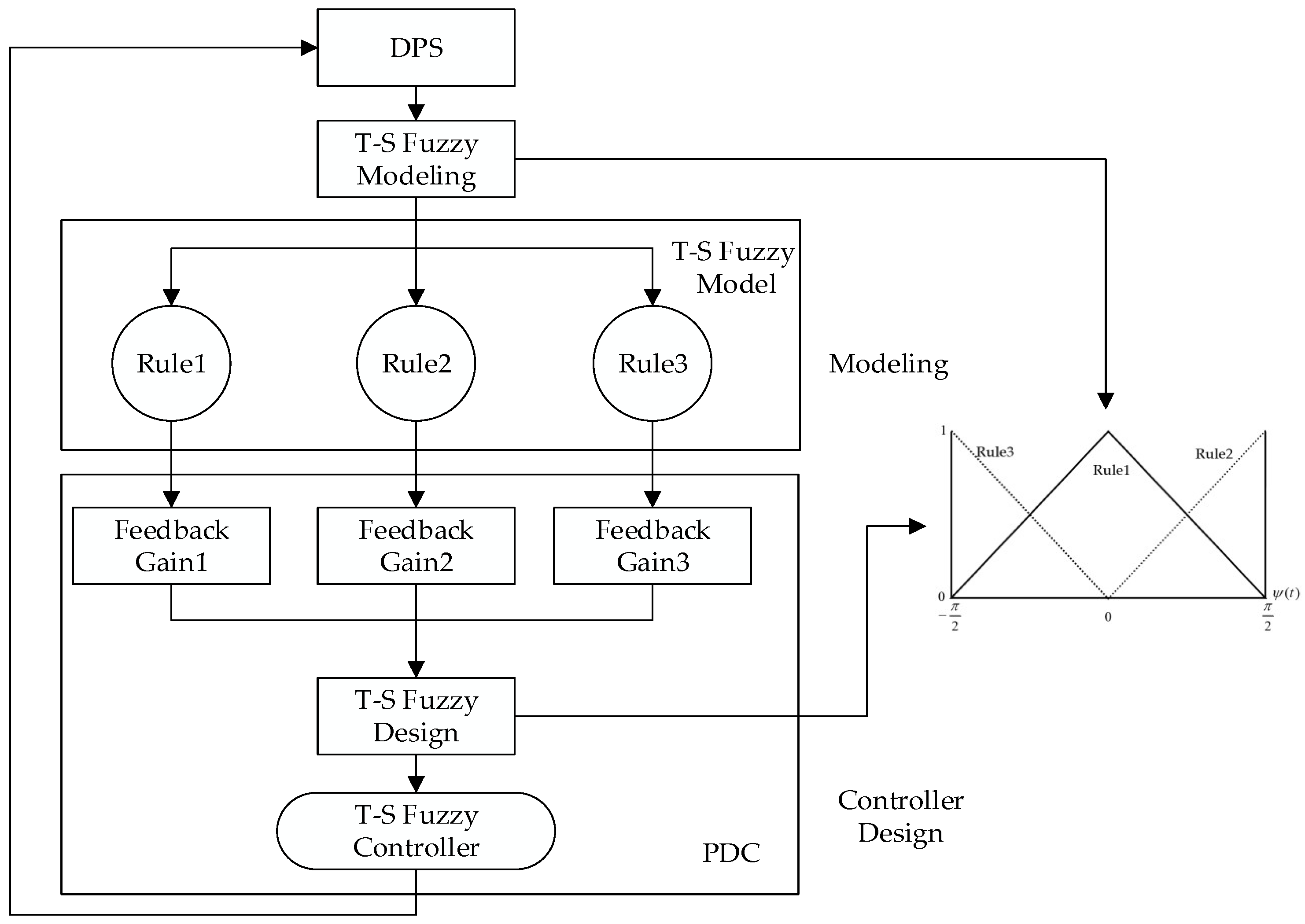
3.2. Introduction of Fuzzy Framework

Using Lemma 1, it can be obtained that

$$\begin{array}{ll}0& =2{\displaystyle \sum _{i=1}^r{\displaystyle \sum _{j=1}^r{\mu }_i(z(t)){\mu }_j(z(t_k)){\xi }^T(t)N_{ij}}}\times [\tau (t)x(t)-{\displaystyle {\int }_{t_k}^{t}x(s)ds}-{\displaystyle {\int }_{-\tau (t)}^0{\displaystyle {\int }_{t+\alpha }^t\dot{x}(s)dsd\alpha }}]\\ & \le 2\tau (t){\displaystyle \sum _{i=1}^r{\displaystyle \sum _{j=1}^r{\mu }_i(z(t)){\mu }_j(z(t_k)){\xi }^T(t)N_{ij}x(t)}}\\ & -2{\displaystyle \sum _{i=1}^r{\displaystyle \sum _{j=1}^r{\mu }_i(z(t)){\mu }_j(z(t_k))}}{\xi }^T(t)N_{ij}{\displaystyle {\int }_{t_k}^{t}x(s)ds}\\ & +\frac{{\tau }^2(t)}{2}{\displaystyle \sum _{i=1}^r{\displaystyle \sum _{j=1}^r{\mu }_i(z(t)){\mu }_j(z(t_k)){\xi }^T(t)N_{ij}{Z}^{-1}{N}_{ij}^T\xi (t)}}\\ & +\frac{2}{{\tau }^2(t)}\left[{\displaystyle {\int }_{-\tau (t)}^0{\displaystyle {\int }_{t+\alpha }^t{\dot{x}}^T(s)dsd\alpha }}\right]Z\left[{\displaystyle {\int }_{-\tau (t)}^0{\displaystyle {\int }_{t+\alpha }^t\dot{x}(s)dsd\alpha }}\right]\\ & \le 2\tau (t){\displaystyle \sum _{i=1}^r{\displaystyle \sum _{j=1}^r{\mu }_i(z(t)){\mu }_j(z(t_k)){\xi }^T(t)N_{ij}x(t)}}\\ & -2{\displaystyle \sum _{i=1}^r{\displaystyle \sum _{j=1}^r{\mu }_i(z(t)){\mu }_j(z(t_k))}}{\xi }^T(t)N_{ij}{\displaystyle {\int }_{t_k}^{t}x(s)ds}\\ & +\frac{{\tau }^2(t)}{2}{\displaystyle \sum _{i=1}^r{\displaystyle \sum _{j=1}^r{\mu }_i(z(t)){\mu }_j(z(t_k)){\xi }^T(t)N_{ij}{Z}^{-1}{N}_{ij}^T\xi (t)}}\\ & +{\displaystyle {\int }_{-\tau (t)}^0{\displaystyle {\int }_{t+\alpha }^t{\dot{x}}^T(s)Z\dot{x}(s)dsd\alpha }}\end{array}$$

(24)

which implies

$$\begin{array}{c}{\displaystyle {\int }_{-\tau (t)}^0{\displaystyle {\int }_{t+\alpha }^t\dot{x}(s)Z\dot{x}(s)dsd\alpha }}\le {\displaystyle \sum _{i=1}^3{\displaystyle \sum _{j=1}^3{\mu }_i(z(t)){\mu }_j(z(t_k))}}\\ \left[2\tau (t){\xi }^T(t)N_{ij}x(t)-2{\xi }^T(t)N_{ij}{\displaystyle {\int }_{t_k}^{t}x(s)ds}\right.\\ \left.+\frac{d\tau (t)}{2}{\xi }^T(t)N_{ij}{Z}^{-1}{N}_{ij}^T\xi (t)\right]\end{array}$$

(25)

Combine (23) with (25) such that

$$\begin{array}{ll}{\dot{V}}_4(t)& \le \frac{d}{4}d(t){\dot{x}}^T(t)Z\dot{x}(t)+\frac{d}{4}\tau (t){\dot{x}}^T(t)Z\dot{x}(t)-\frac{d(t)}{d}{\left[\begin{array}{c}x(t_k)\\ x(t)\end{array}\right]}^T\left[\begin{array}{cc}Z& -Z\\ -Z& Z\end{array}\right]\left[\begin{array}{c}x(t_k)\\ x(t)\end{array}\right]\\ & +{\displaystyle \sum _{i=1}^3{\displaystyle \sum _{j=1}^3{\mu }_i(z(t)){\mu }_j(z(t_k))\left[2\tau (t){\xi }^T(t)N_{ij}x(t)\right.}}\\ & \left.-2{\xi }^T(t)N_{ij}{\displaystyle {\int }_{t_k}^{t}x(s)ds}+\frac{d\tau (t)}{2}{\xi }^T(t)N_{ij}{Z}^{-1}{N}_{ij}^T\xi (t)\right]\end{array}$$

(26)

For any matrixes $G,$$M_{ij},i,j\in L$ and scalars ${\epsilon }_i,i=1,2,3,4$, we have

$$0={\displaystyle \sum _{i=1}^3{\displaystyle \sum _{j=1}^3{\mu }_i(z(t)){\mu }_j(z(t_k)){\xi }^T(t)M_{ij}}}\times \left[x(t)-x(t_k)-{\displaystyle {\int }_{t_k}^t\dot{x}(s)ds}\right]$$

(27)

$$\begin{array}{l}0=2\left[{\epsilon }_1{x}^T(t)G+{\epsilon }_2{\dot{x}}^T(t)G+{\epsilon }_{3}x(t_k)G+{\epsilon }_4{\displaystyle {\int }_{t_k}^t{x}^T(s)Gds}\right]\\ \times \left[-\dot{x}(t)+{\displaystyle \sum _{i=1}^3{\displaystyle \sum _{j=1}^3{\mu }_i(z(t)){\mu }_j(z(t_k))\left(A_{i}x(t)+B_i{K}_{j}x(t_k)\right)}}\right]\end{array}$$

(28)

From (22), (23) and (26)–(28), we obtain that

$$\begin{array}{l}\dot{V}(t)\le \frac{d(t)}{d}{\displaystyle \sum _{i=1}^3{\displaystyle \sum _{j=1}^3{\mu }_i(z(t)){\mu }_j(z(t_k)){\xi }^T(t){\mathsf{\Psi }}_3^{ij}\xi (t)}}\\ +\frac{1}{d}{\displaystyle \sum _{i=1}^3{\displaystyle \sum _{j=1}^3{\mu }_i(z(t)){\mu }_j(z(t_k)){{\displaystyle {\int }_{t_k}^t\left[\begin{array}{c}\xi (t)\\ \dot{x}(s)\end{array}\right]}}^T{\widehat{\mathsf{\Psi }}}_4^{ij}\left[\begin{array}{c}\xi (t)\\ \dot{x}(s)\end{array}\right]ds}}\end{array}$$

(29)

where

$$\begin{array}{l}{\widehat{\mathsf{\Psi }}}_4^{ij}=\left[\begin{array}{cc}{\mathsf{\Pi }}_{11ij}& {\mathsf{\Theta }}_{ij}\\ \ast & -dQ-R_{11}\end{array}\right]+\frac{d^2}{2}\left[\begin{array}{c}{N}_{ij}\\ 0\end{array}\right]Z^{-1}{\left[\begin{array}{c}{N}_{ij}\\ 0\end{array}\right]}^T\\ {\mathsf{\Theta }}_{ij}={\left[\begin{array}{cccc}-d{M}_{1ij}^T& -d{M}_{2ij}^T& -d{R}_{12}-d{M}_{3ij}^T& -d{M}_{4ij}^T\end{array}\right]}^T\end{array}$$

(30)

Following the Schur complement, (30) implies ${\widehat{\mathsf{\Psi }}}_4^{ij}<0$. It can be referred that $\dot{V}\left(t\right)<-\sigma {\parallel x\left(t\right)\parallel }^2$ when

$x\left(t\right)\ne 0,\sigma >0$, which shows that the system (11) is asymptotically stable. This proof is completed.

Remark 2.

To fully capture the available characteristics of sampling patterns, some novel terms, like$d(t){\displaystyle {\int }_{-d(t)}^0{\displaystyle {\int }_{t+\theta }^t\dot{x}{(s)}^{T}Z\dot{x}(s)dsd\theta }}$, have been introduced in the LKF, which means that the constructed LKF is general.

Remark 3.

Compared with the LKF in [38,39], more available matrices, such as $Q,R,X,U$, are effectively used in the LKF. If we let $R_{12}=R_{22}=Z=Q=0$ and $U_{13}=U_{12}=U_{22}=X_{13}=X_{23}=X_{33}=0$, the LKF will be reduced to those in [38,39], which means that the proposed LKF has a more general form. Moreover, free matrices $M_{ij}$ and $N_{ij}$ are introduced into the differentiation of the LKF. Hence, model transformation and bounding techniques are avoided, which overcomes an important source of conservatism.

Remark 4.

In the process of derivative and further proof of the LKF in [38,39], the positive definite requirement of the matrix is necessary. In this paper, X-dependent terms are introduced in $V_1(t)$ and are not required to be positive definite, which means that the limitation conditions of the matrices are overcome. Hence, the conservativeness can be further reduced.

3.3. Design of Sampled-Data Controller

Theorem 2.

Given scalars $d>0$ and ${\epsilon }_i,i=1,2,3,4$, the system (15) is asymptotically stable, if there exist symmetric matrices $P>0,Q>0,Z>0,$ $\left[\begin{array}{cc}{R}_{11}& R_{12}\\ \ast & R_{22}\end{array}\right]>0,\left[\begin{array}{cc}{U}_{11}& U_{12}\\ \ast & U_{22}\end{array}\right]>0,X_{11},X_{13},X_{22},X_{23},X_{33},G,$ $M_{ij}={\left[\begin{array}{cccc}{M}_{1ij}^T& M_{2ij}^T& M_{3ij}^T& M_{4ij}^T\end{array}\right]}^T,N_{ij}={\left[\begin{array}{cccc}{N}_{1ij}^T& N_{2ij}^T& N_{3ij}^T& N_{4ij}^T\end{array}\right]}^T,$such that

$${\mathsf{\Psi }}_1^{ij}=\left[\begin{array}{ccc}P+d\left(X_{11}+X_{11}^T+Q\right)& d\left(X_{11}+X_{22}-Q\right)& d{X}_{13}\\ \ast & d\left(X_{11}+X_{22}^T+Q\right)& d{X}_{23}\\ \ast & \ast & d{X}_{33}\end{array}\right]>0$$

(31)

$${\tilde{\mathsf{\Psi }}}_2^{ij}=\left[\begin{array}{cccc}{\tilde{\mathsf{\Xi }}}_{11}^{ij}+{\tilde{\mathsf{\Omega }}}_{11}^{ij}& {\tilde{\mathsf{\Xi }}}_{12}^{ij}+{\tilde{\mathsf{\Omega }}}_{12}^{ij}& {\tilde{\mathsf{\Xi }}}_{13}^{ij}+{\tilde{\mathsf{\Omega }}}_{13}^{ij}& {\tilde{\mathsf{\Xi }}}_{14}^{ij}+d{X}_{33}^T\\ \ast & {\tilde{\mathsf{\Xi }}}_{22}^{ij}+{\tilde{\mathsf{\Omega }}}_{22}^{ij}& {\tilde{\mathsf{\Xi }}}_{23}^{ij}+{\tilde{\mathsf{\Omega }}}_{23}^{ij}& {\tilde{\mathsf{\Xi }}}_{24}^{ij}+d{X}_{13}\\ \ast & \ast & {\tilde{\mathsf{\Xi }}}_{33}^{ij}+{\tilde{\mathsf{\Omega }}}_{33}^{ij}& {\tilde{\mathsf{\Xi }}}_{34}^{ij}\\ \ast & \ast & \ast & {\tilde{\mathsf{\Xi }}}_{44}^{ij}\end{array}\right]<0$$

(32)

$${\mathsf{\Psi }}_3^{ij}=\left[\begin{array}{cc}{\tilde{\mathsf{\Pi }}}_{11ij}& {\tilde{\mathsf{\Pi }}}_{12ij}\\ \ast & {\tilde{\mathsf{\Pi }}}_{22}\end{array}\right]<0,$$

(33)

where

$$\begin{array}{l}{\tilde{\mathsf{\Pi }}}_{11ij}=\left[\begin{array}{cccc}{\tilde{\mathsf{\Xi }}}_{11}^{ij}+{\tilde{\mathsf{\Omega }}}_{11}^{ij}& {\tilde{\mathsf{\Xi }}}_{12}^{ij}+d{\tilde{N}}_{2ij}^T& {\tilde{\mathsf{\Xi }}}_{13}^{ij}+d{\tilde{N}}_{3ij}^T& {\tilde{\mathsf{\Xi }}}_{14}^{ij}+d{\tilde{N}}_{4ij}^T\\ \ast & {\tilde{\mathsf{\Xi }}}_{22}^{ij}+\frac{d^2}{4}\tilde{Z}& {\tilde{\mathsf{\Xi }}}_{23}^{ij}& {\tilde{\mathsf{\Xi }}}_{24}^{ij}\\ \ast & \ast & {\tilde{\mathsf{\Xi }}}_{33}^{ij}+{\tilde{\mathsf{\Omega }}}_{33}^{ij}& {\tilde{\mathsf{\Xi }}}_{34}^{ij}\\ \ast & \ast & \ast & {\tilde{\mathsf{\Xi }}}_{44}^{ij}\end{array}\right],\\ {\tilde{\mathsf{\Pi }}}_{12ij}=\left[\begin{array}{cc}-d{\tilde{M}}_{1ij}& d{\tilde{N}}_{1ij}\\ -d{\tilde{M}}_{2ij}& d{\tilde{N}}_{2ij}\\ -d{\tilde{R}}_{12}^T-d{\tilde{M}}_{3ij}& d{\tilde{N}}_{3ij}\\ -d{\tilde{M}}_{4ij}& d{\tilde{N}}_{4ij}\end{array}\right],{\tilde{\mathsf{\Pi }}}_{22}=\left[\begin{array}{cc}-d\tilde{Q}-d{\tilde{R}}_{11}& 0\\ \ast & -2\tilde{Z}\end{array}\right],\\ {\tilde{\mathsf{\Xi }}}_{11}^{ij}=-{\tilde{X}}_{11i}-{\tilde{X}}_{11i}^T+{\tilde{M}}_{1ij}^T+{\tilde{M}}_{1ij}-{\epsilon }_1{A}_i{\tilde{G}}^T-{\epsilon }_1\tilde{G}{A}_i^T\\ {\tilde{\mathsf{\Xi }}}_{12}^{ij}=P+{\tilde{M}}_{2ij}^T+{\epsilon }_1\tilde{G}-{\epsilon }_2{A}_i^T{\tilde{G}}^T\\ {\tilde{\mathsf{\Xi }}}_{13}^{ij}={\tilde{X}}_{11i}+{\tilde{X}}_{22i}+{\tilde{M}}_{3ij}^T-{\tilde{M}}_{1ij}-{\epsilon }_1{B}_i{\tilde{K}}_j-{\epsilon }_3\tilde{G}{A}_i^T\\ {\tilde{\mathsf{\Xi }}}_{14}^{ij}=-{\tilde{X}}_{13i}+{\tilde{M}}_{4ij}^T-{\tilde{N}}_{1ij}-{\epsilon }_4\tilde{G}{A}_i^T\\ {\tilde{\mathsf{\Xi }}}_{22}^{ij}={\epsilon }_2\tilde{G}+{\epsilon }_2{\tilde{G}}^T\\ {\tilde{\mathsf{\Xi }}}_{23}^{ij}=-{\tilde{M}}_{2ij}-B_i{\tilde{K}}_j+{\epsilon }_3\tilde{G}\\ {\tilde{\mathsf{\Xi }}}_{24}^{ij}={\epsilon }_4{\tilde{G}}^T-{\tilde{N}}_{2ij}\\ \end{array}$$

$$\begin{array}{l}{\tilde{\mathsf{\Xi }}}_{33}^{ij}=-{\tilde{X}}_{22i}-{\tilde{X}}_{22i}^T-{\tilde{M}}_{3ij}^T-{\tilde{M}}_{3ij}-{\epsilon }_3{B}_i{\tilde{K}}_j-{\epsilon }_3{\tilde{K}}_j^T{B}_i^T\\ {\tilde{\mathsf{\Xi }}}_{34}^{ij}=-{\tilde{X}}_{23i}-{\tilde{U}}_{12}-{\tilde{M}}_{4ij}^T-N_{3ij}-{\epsilon }_4{\tilde{K}}_j^T{B}_i^T\\ {\tilde{\mathsf{\Xi }}}_{44}^{ij}=-{\tilde{X}}_{33i}-\frac{1}{d}{\tilde{U}}_{22}-{\tilde{N}}_{4ij}^T-{\tilde{N}}_{4ij}\\ {\tilde{\mathsf{\Omega }}}_{11}=d\left({\tilde{X}}_{13}+{\tilde{X}}_{13}^T\right)+d{\tilde{U}}_{22}-\tilde{Z}\\ {\tilde{\mathsf{\Omega }}}_{12}=d{\tilde{X}}_{11}+d{\tilde{X}}_{11}^T\\ {\tilde{\mathsf{\Omega }}}_{13}=d{\tilde{X}}_{23}^T+d{\tilde{U}}_{12}^T+\tilde{Z}\\ {\tilde{\mathsf{\Omega }}}_{22}=d{\tilde{R}}_{11}+d\tilde{Q}+\frac{d^2}{4}\tilde{Z}\\ {\tilde{\mathsf{\Omega }}}_{23}=-d\left({\tilde{X}}_{11}+{\tilde{X}}_{22}\right)+d{\tilde{R}}_{12}\\ {\tilde{\mathsf{\Omega }}}_{33}=d{\tilde{R}}_{22}+d{\tilde{U}}_{11}-\tilde{Z}\\ \end{array}$$

The fuzzy controller is obtained that

$$K_j={\tilde{K}}_j{\tilde{G}}^{-T}$$

(34)

Proof. 

Denoting

$$\begin{array}{l}\tilde{G}=G^{-1},{\tilde{K}}_j=K_j{\tilde{G}}^T,{\tilde{P}}_i=\tilde{G}{P}_i{\tilde{G}}^T,{\tilde{X}}_{11i}=\tilde{G}{X}_{11}{\tilde{G}}^T,\\ {\tilde{X}}_{22i}=\tilde{G}{X}_{22}{\tilde{G}}^T,{\tilde{X}}_{13i}=\tilde{G}{X}_{13i}{\tilde{G}}^T,{\tilde{X}}_{23i}=\tilde{G}{X}_{23i}{\tilde{G}}^T,\\ {\tilde{X}}_{33i}=\tilde{G}{X}_{33i}{\tilde{G}}^T,{\tilde{R}}_{11}=\tilde{G}{R}_{11}{\tilde{G}}^T,{\tilde{R}}_{12}=\tilde{G}{R}_{12}{\tilde{G}}^T,\\ {\tilde{R}}_{22}=\tilde{G}{R}_{22}{\tilde{G}}^T,\tilde{Q}=\tilde{G}Q{\tilde{G}}^T,{\tilde{U}}_{11}=\tilde{G}{U}_{11}{\tilde{G}}^T,{\tilde{U}}_{12}=\tilde{G}{U}_{12}{\tilde{G}}^T,\\ {\tilde{U}}_{22}=\tilde{G}{U}_{22}{\tilde{G}}^T,\tilde{Z}=\tilde{G}Z{\tilde{G}}^T,{\mathsf{\Gamma }}_1=diag\left\{\tilde{G},\tilde{G},\tilde{G}\right\},\\ {\mathsf{\Gamma }}_2=diag\left\{\tilde{G},\tilde{G},\tilde{G},\tilde{G}\right\},{\mathsf{\Gamma }}_3=diag\left\{\tilde{G},\tilde{G},\tilde{G},\tilde{G},\tilde{G},\tilde{G}\right\},\\ {\tilde{M}}_{ij}={\mathsf{\Gamma }}_2{M}_{ij}{\mathsf{\Gamma }}_2^T,{\tilde{N}}_{ij}={\mathsf{\Gamma }}_2{N}_{ij}{\mathsf{\Gamma }}_2^T.\\ \end{array}$$

Pre- and post-multiplying (18), (19), (20) by ${\mathsf{\Gamma }}_1,{\mathsf{\Gamma }}_2,{\mathsf{\Gamma }}_3$ and ${\mathsf{\Gamma }}_1^T,{\mathsf{\Gamma }}_2^T,{\mathsf{\Gamma }}_3^T$, respectively, (31), (32), (33) are obtained. This completed the proof. □

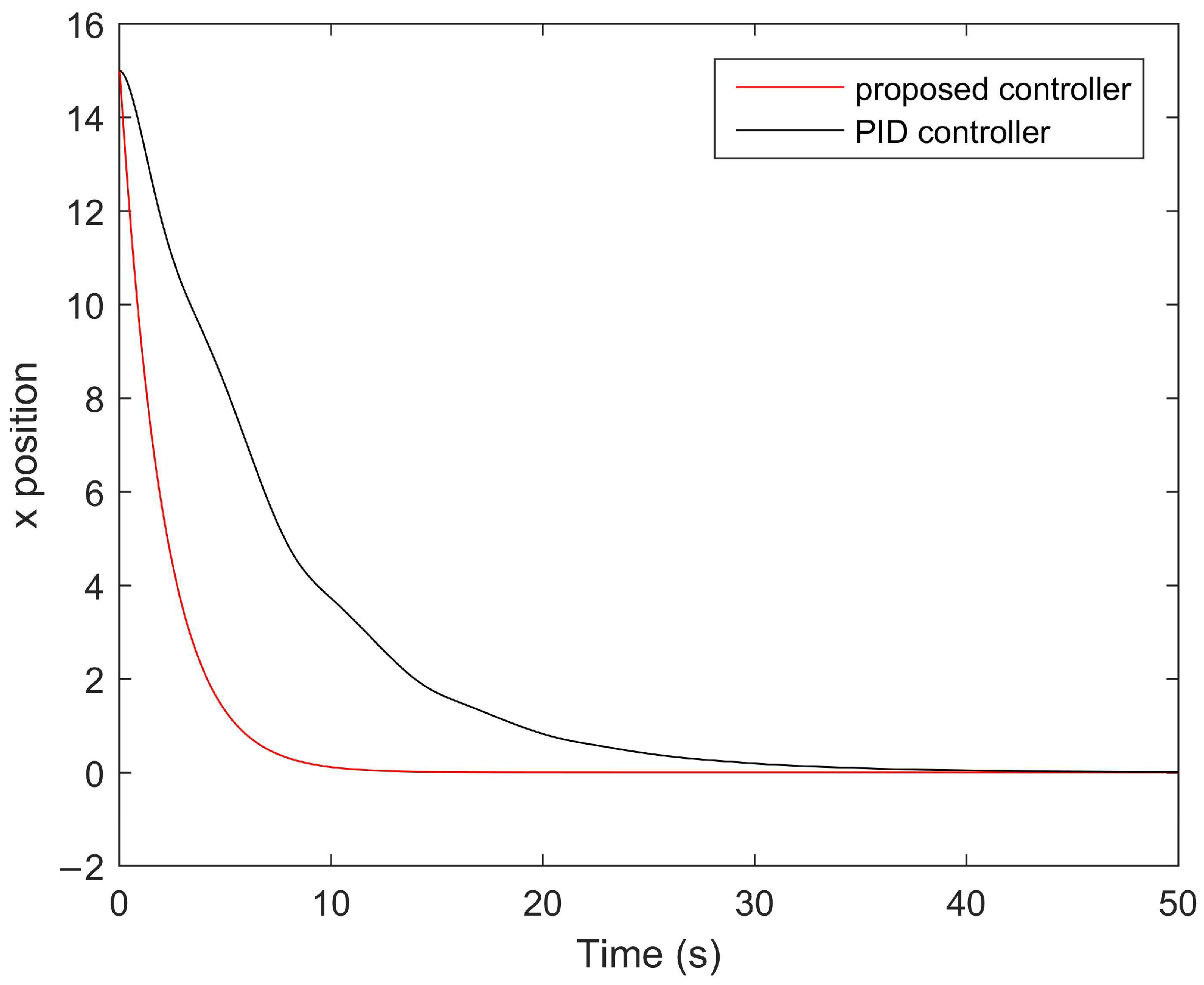
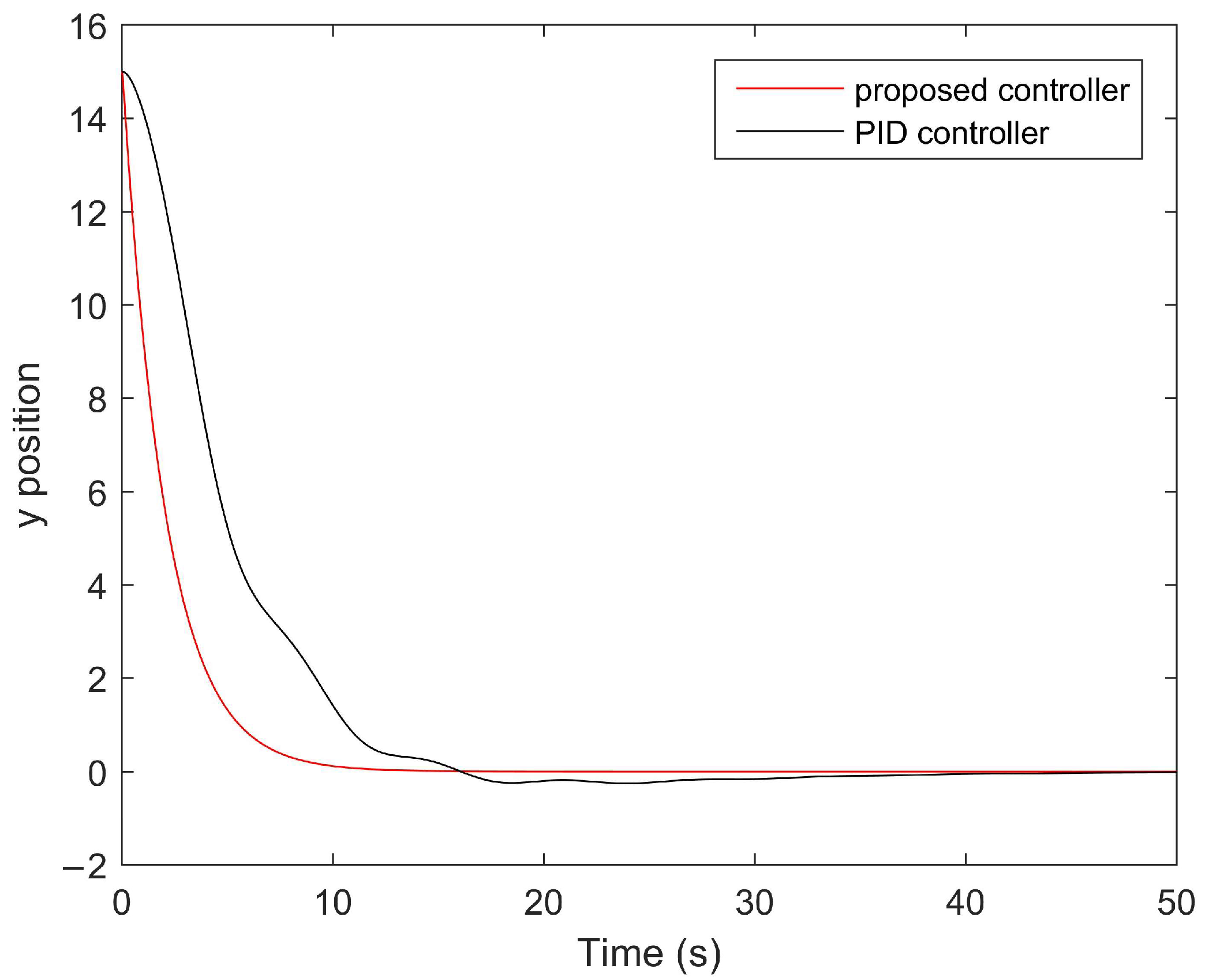
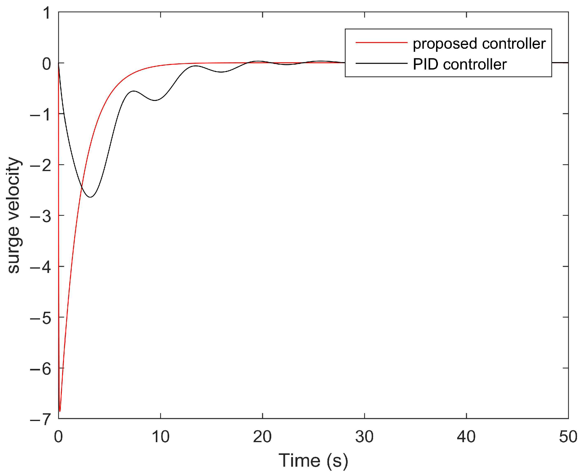
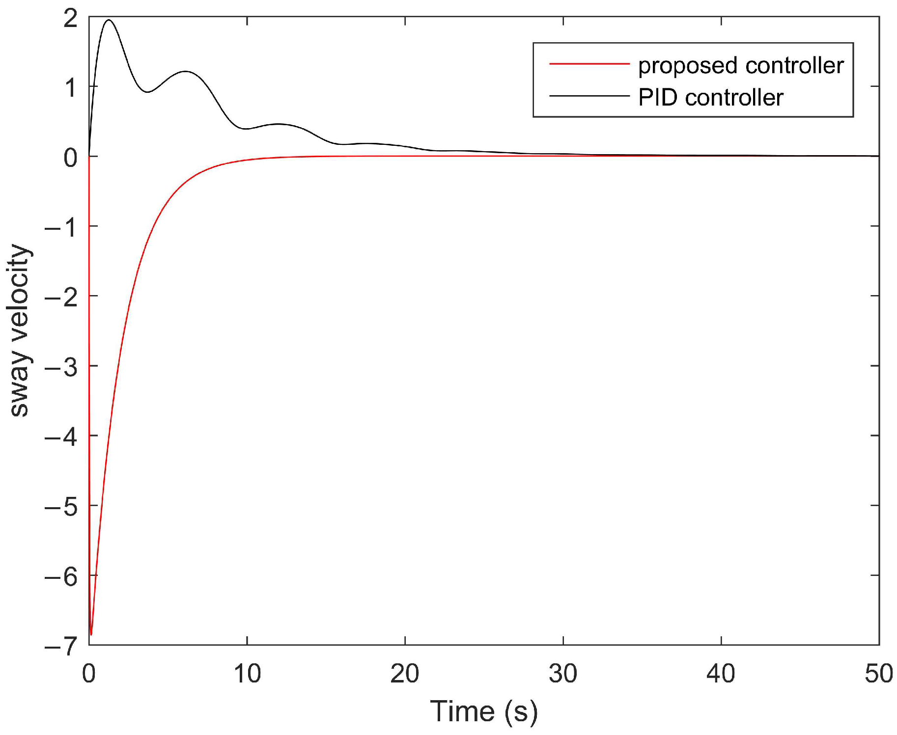
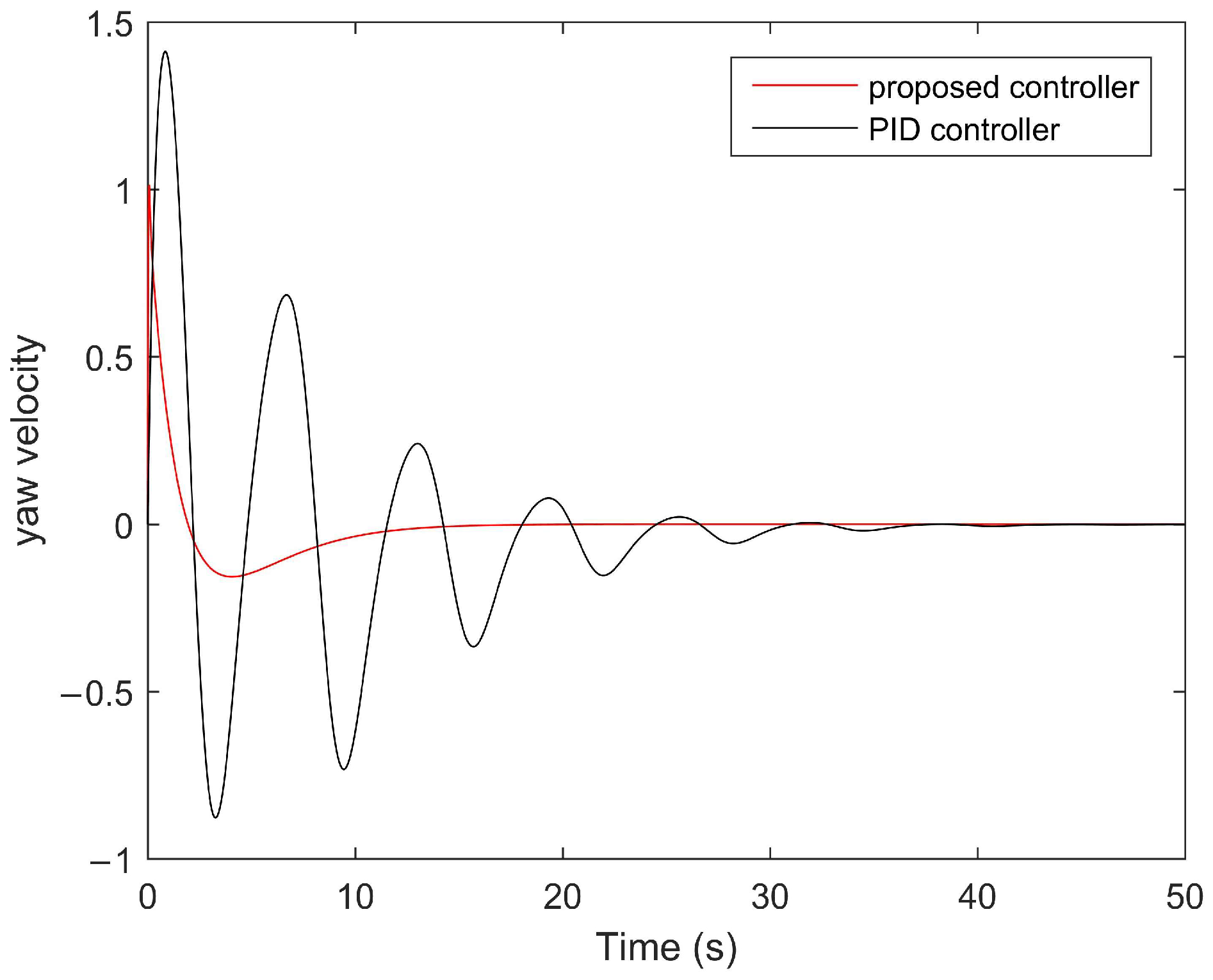
4. Numerical Examples

In this section, an application example of a DPS is introduced to show the superiority of the methods. M, D and G are considered as follows [41].

$$\begin{array}{l}M=\left[\begin{array}{ccc}1.0852& 0& 0\\ 0& 2.0575& -0.4087\\ 0& -0.4087& 0.2153\end{array}\right],D=\left[\begin{array}{ccc}0.0865& 0& 0\\ 0& 0.0762& 0.1510\\ 0& 0.0151& 0.0031\end{array}\right],\\ G=\left[\begin{array}{ccc}0.0389& 0& 0\\ 0& 0.0266& 0\\ 0& 0& 0\end{array}\right].\\ \end{array}$$

Let $\alpha =\sin 2^0$ and $\beta =\cos {88}^0$, we have

$$\begin{array}{l}{A}_1=\left[\begin{array}{cccccc}0& 0& 0& 1.0000& -0.0349& 0\\ 0& 0& 0& 0.0349& 1.0000& 0\\ 0& 0& 0& 0& 0& 1.0000\\ -0.0358& 0& 0& -0.0797& 0& 0\\ 0& -0.0208& 0& 0& -0.0818& -0.1224\\ 0& -0.0394& 0& 0& -0.2254& -0.2468\end{array}\right],\\ A_2=\left[\begin{array}{cccccc}0& 0& 0& 0.0349& -1.0000& 0\\ 0& 0& 0& 1.0000& 0.0349& 0\\ 0& 0& 0& 0& 0& 1.0000\\ -0.0358& 0& 0& -0.0797& 0& 0\\ 0& -0.0208& 0& 0& -0.0818& -0.1224\\ 0& -0.0394& 0& 0& -0.2254& -0.2468\end{array}\right],\\ A_3=\left[\begin{array}{cccccc}0& 0& 0& 0.0349& 1.0000& 0\\ 0& 0& 0& -1.0000& 0.0349& 0\\ 0& 0& 0& 0& 0& 1.0000\\ -0.0358& 0& 0& -0.0797& 0& 0\\ 0& -0.0208& 0& 0& -0.0818& -0.1224\\ 0& -0.0394& 0& 0& -0.2254& -0.2468\end{array}\right],\\ B_i=\left[\begin{array}{ccc}0& 0& 0\\ 0& 0& 0\\ 0& 0& 0\\ 0.9215& 0& 0\\ 0& 0.7802& 1.4811\\ 0& 1.4811& 7.4562\end{array}\right],i=1,2,3.\end{array}$$

Firstly, we compare the proposed method with references that used traditional T-S fuzzy models. From

Table 1. Maximum values of the upper sampling internal.

Method	[37]	[38]	[39]	Theorem 1
d2	0.25	0.264	0.532	0.681

, the maximum sampling internal is $d=0.681$. Note that results in [37,38,39] are 0.25, 0.264, and 0.532, respectively. This means that the sampling internal in this paper improves [37,38,39] by 160.8, 146.97, and 22.56%, respectively. It also shows that the proposed controllers play an important role in obtaining a longer sampling interval.

Next, we combined references that used different methods, such as T-set [42], Pareto optimality under T-set [43], and intuitionistic fuzzy T-set [44], to obtain the maximum sampling internal. In

Table 2. Maximum values of the upper sampling internal.

Technologies	Maximum Sampling Internal
T-set	0.583
Pareto optimality under T-set	0.624
Intuitionistic fuzzy T-set	0.652
Proposed method	0.681

, we can see that the values of the obtained sampling internal were close to the method proposed in this paper, which illustrates that the technology derived from the T-set has its advantages. And T-sets can be used to replace fuzzy sets to represent uncertainty.

The initial values are chosen that $x_s(t)=\left[\begin{array}{cccccc}15\mathrm{m}& 15\mathrm{m}& 0.2°& 0\mathrm{m}/\mathrm{s}& 0\mathrm{m}/\mathrm{s}& 0°\end{array}\right]$.

And the other parameters are $d=1.6\mathrm{s},{\epsilon }_1={\epsilon }_2=1,{\epsilon }_3={\epsilon }_4=0$. Then, the gain can be computed that

$$\begin{array}{l}{K}_1=\left[\begin{array}{cccccc}-0.0260& -0.0387& -0.0309& -0.6802& -0.0002& -0.0004\\ 0.0619& -0.0067& 0.0395& 0.0004& -1.3157& 0.2556\\ -0.0124& 0.0061& 0.0066& -0.0001& 0.2653& -0.1315\end{array}\right]\\ K_2=\left[\begin{array}{cccccc}-0.0123& 0.0143& 0.0154& -0.7071& -0.0002& 0.0000\\ -0.0196& 0.0251& 0.0698& 0.0003& -1.3667& 0.2643\\ 0.0041& -0.0002& 0.0011& -0.0001& 0.2754& -0.1364\end{array}\right]\\ K_3=\left[\begin{array}{cccccc}-0.0123& 0.0143& 0.0154& -0.7071& -0.0002& 0.0000\\ -0.0196& 0.0251& 0.0698& 0.0003& -1.3667& 0.2643\\ 0.0041& -0.0002& 0.0011& -0.0001& 0.2754& -0.1364\end{array}\right]\end{array}$$

To illustrate the control performance of the proposed approaches, comparison results with those of the PID controller [45] are presented in Figure 4, Figure 5, Figure 6, Figure 7, Figure 8 and Figure 9.

The PID value was chosen such that

$$\begin{array}{l}{K}_p=diag\left([2.8\times {10}^3,6\times {10}^3,2.3\times {10}^6]\right)\\ K_p=diag\left([1,1,1]\right)\\ K_p=diag\left([4.5\times {10}^4,3.5\times {10}^4.1\times {10}^4]\right)\end{array}$$

In Figure 4, Figure 5, Figure 6, Figure 7, Figure 8 and Figure 9 it is shown that the ship’s position, yaw angle, and velocities reached expected values within about 10 s, while under the PID controller designed in [39], it took longer to reach the predetermined targets, which means that the designed method in this paper, which used the proposed method, has a faster response speed. In addition, this demonstrates that the oscillation amplitude of the system is relatively small, indicating that the designed controllers have good anti-interference ability. Meanwhile, Figure 4, Figure 5, Figure 6, Figure 7, Figure 8 and Figure 9 further indicate that the designed sampled-data controller also has a relatively fast speed response time, which means that the controller has fast convergence speed and high stability.

5. Conclusions

This article investigated DPS stabilization problems using sampled-data under T-S fuzzy models. To reduce the conservatism of the obtained results, some novel terms were introduced in the constructed LKF, and a larger sampling interval was achieved. The main novelty of the LKF is that the sampling mode information is fully utilized; in addition, the positive definite constraints of LKFs are relaxed, and additional free matrices are provided to further reduce the conservatism. Experimental results showed that the developed control methods are superior. In the future, we will explore using the T-set method instead of the fuzzy set to represent real-life scenarios and fully consider the characteristics of linear time-varying systems [46], which will become a new topic in future work.

References

1. Fossen, T.I. Guidance and Control of Ocean Vehicles; Wiley: New York, NY, USA, 1994. [Google Scholar]
2. Wang, Y.L.; Han, Q.L.; Fei, M.R.; Peng, C. Network-based T-S fuzzy dynamic positioning controller design for unmanned marine vehicles. IEEE Trans. Cybern. 2018, 48, 2750–2763. [Google Scholar] [CrossRef]
3. Hao, L.Y.; Zhang, H.; Li, T.S.; Lin, B.; Chen, C.P. Fault tolerant control for dynamic positioning of unmanned marine vehicles based on T-S fuzzy model with unknown membership functions. IEEE Trans. Veh. Technol. 2021, 70, 146–157. [Google Scholar] [CrossRef]
4. Veksler, A.; Johansen, T.A.; Borrelli, F.; Realfsen, B. Dynamic positioning with model predictive control. IEEE Trans. Control Syst. Technol. 2016, 24, 1340–1353. [Google Scholar] [CrossRef]
5. Nguyen, V.S. Investigation of a multitasking system for automatic ship berthing in marine practice based on an integrated neural controller. Mathematics 2020, 8, 1167. [Google Scholar] [CrossRef]
6. Benetazzo, F.; Ippoliti, G.; Longhi, S.; Raspa, P. Advanced control for fault-tolerant dynamic positioning of an offshore supply vessel. Ocean Eng. 2015, 106, 472–484. [Google Scholar] [CrossRef]
7. Karimi, H.R.; Lu, Y. Guidance and control methodologies for marine vehicles: A survey. Control Eng. Pract. 2021, 111, 104785. [Google Scholar] [CrossRef]
8. Wang, Y.; Yang, X.; Yan, H. Reliable fuzzy tracking control of near-space hypersonic vehicle using aperiodic measurement information. IEEE Trans. Ind. Electron. 2019, 66, 9439–9447. [Google Scholar] [CrossRef]
9. Karimi, H.R. Robust H∞ filter design for uncertain linear systems over network with network-induced delays and output quantization. Nor. Foren. Autom. 2009, 30, 27–37. [Google Scholar] [CrossRef]
10. Kiruthika, R.; Krishnasamy, R.; Lakshmanan, S.; Prakash, M.; Manivannan, A. Non-fragile sampled-data control for synchronization of chaotic fractional-order delayed neural networks via LMI approach. Chaos Solitons Fractals 2023, 169, 113252. [Google Scholar] [CrossRef]
11. Wang, Y.; Xia, Y.; Zhou, P. Fuzzy-model-based sampled-data control of chaotic systems: A fuzzy time-dependent Lyapunov–Krasovskii functional approach. IEEE Trans. Fuzzy Syst. 2016, 25, 1672–1684. [Google Scholar] [CrossRef]
12. Wang, Y.; Shi, P. On master-slave synchronization of Chaotic Lur’e systems using sampled-data control. IEEE Trans. Circuits Syst. II Express Briefs 2016, 85, 981–992. [Google Scholar] [CrossRef]
13. Chen, W.-H.; Wang, Z.; Lu, X. On sampled-data control for masterslave synchronization of chaotic Lur’e systems. IEEE Trans. Circuits Syst. II Express Briefs 2012, 59, 515–519. [Google Scholar]
14. Wu, Z.-G.; Shi, P.; Su, H.; Chu, J. Local synchronization of chaotic neural networks with sampled-data and saturating actuators. IEEE Trans. Cybern. 2014, 44, 2635–2645. [Google Scholar]
15. Wu, Z.G.; Shi, P.; Su, H.Y. Stochastic Synchronization of Markovian Jump Neural Networks with Time-Varying Delay Using Sampled Data. IEEE Trans. Cybern. 2013, 43, 796–1806. [Google Scholar] [CrossRef] [PubMed]
16. Karimi, H.R.; Gao, H. Mixed H2/H∞ output-feedback control of second-order neutral systems with time-varying state and input delays. ISA Trans. 2008, 47, 311–324. [Google Scholar] [CrossRef]
17. Wei, Y.; Karimi, H.R.; Yang, S. New results on sampled-data output-feedback control of linear parameter-varying systems. Int. J. Robust Nonlinear Control 2022, 32, 5070–5085. [Google Scholar] [CrossRef]
18. Li, S.; Yang, L.; Li, K.; Gao, Z. Robust sampled-data cruise control scheduling of high speed train. Transp. Res. Part C Emerg. Technol. 2014, 46, 274–283. [Google Scholar] [CrossRef]
19. Wang, Y.; Wang, Q.; Zhou, P.; Duan, D. Robust H∞ directional control for a sampled-data autonomous airship. J. Cent. South Univ. 2014, 21, 1339–1346. [Google Scholar] [CrossRef]
20. Zheng, M.; Zhou, Y.; Yang, S.; Li, L. Robust H∞ control of neutral system for sampled-data dynamic positioning ships. IMA J. Math. Control Inf. 2019, 36, 1325–1345. [Google Scholar] [CrossRef]
21. Zou, Z.; Zheng, M. Design and stabilization analysis of luxury cruise with dynamic positioning systems based on sampled-data control. Math. Biosci. Eng. 2023, 20, 14026–14045. [Google Scholar] [CrossRef] [PubMed]
22. Zheng, M.; Su, Y.; Yang, S.; Li, L. Reliable fuzzy dynamic positioning tracking controller for unmanned surface vehicles based on aperiodic measurement information. Int. J. Fuzzy Syst. 2023, 25, 358–368. [Google Scholar] [CrossRef]
23. Castro, M.F.; Seuret, A.; Leite, V.J.; Silva, L.F. Robust local stabilization of discrete time varying delayed state systems under saturating actuators. Automatica 2020, 122, 109266. [Google Scholar] [CrossRef]
24. Ge, G.; Lei, D.; Han, Q. A distributed event-triggered transmission strategy for sampled-data consensus of multi-agent systems. Automatica 2014, 50, 1489–1496. [Google Scholar]
25. Zhang, X.; Han, Q.; Zhang, B. An overview and deep investigation on sampled-data-based event-triggered control and filtering for networked systems. IEEE Trans. Ind. Inform. 2017, 13, 4–16. [Google Scholar] [CrossRef]
26. Yan, L.; Wang, Z.; Zhang, M.; Fan, Y. Sampled-data control for mean-square exponential stabilization of memristive neural networks under deception attacks. Chaos Solitons Fractals 2023, 174, 113787. [Google Scholar] [CrossRef]
27. Yerudkar, A.; Chatzaroulas, E.; Del Vecchio, C.; Moschoyiannis, S. Sampled-data control of probabilistic boolean control networks: A deep reinforcement learning approach. Inf. Sci. 2023, 619, 374–389. [Google Scholar] [CrossRef]
28. Wang, Y.; Karimi, H.R.; Lam, H.K.; Shen, H. An improved result on exponential stabilization of sampled-data fuzzy systems. IEEE Trans. Fuzzy Syst. 2018, 26, 3875–3883. [Google Scholar] [CrossRef]
29. Yan, S.; Gu, Z.; Park, J.H.; Xie, X. Adaptive memory-event-triggered static output control of T–S fuzzy wind turbine systems. IEEE Trans. Fuzzy Syst. 2021, 30, 3894–3904. [Google Scholar] [CrossRef]
30. Cai, X.; Shi, K.; She, K.; Zhong, S.; Tang, Y. Quantized sampled-data control tactic for TS fuzzy NCS under stochastic cyber-attacks and its application to truck-trailer system. IEEE Trans. Veh. Technol. 2022, 71, 7023–7032. [Google Scholar] [CrossRef]
31. Wang, Y.; Xia, Y.; Ahn, C.K.; Zhu, Y. Exponential stabilization of takagi–sugeno fuzzy systems with aperiodic sampling: An aperiodic adaptive event-triggered method. IEEE Trans. Syst. Man Cybern. Syst. 2019, 49, 444–454. [Google Scholar] [CrossRef]
32. Sheng, Z.; Lin, C.; Chen, B.; Wang, Q.-G. Stability and Stabilization of TS Fuzzy Time-delay Systems under Sampled-data Control via New Asymmetric Functional Method. IEEE Trans. Fuzzy Syst. 2023, 31, 3197–3209. [Google Scholar] [CrossRef]
33. Velmurugan, G.; Joo, Y.H. Sampled-Data Control Design for T-S Fuzzy System via Quadratic Function Negative Determination Approach. IEEE Trans. Fuzzy Syst. 2023, 31, 3197–3209. [Google Scholar] [CrossRef]
34. Katayama, H. Nonlinear Sampled-Data Stabilization of Dynamically Positioned Ships. IEEE Trans. Control Syst. Technol. 2010, 18, 463–468. [Google Scholar] [CrossRef]
35. Katayama, H.; Aoki, H. Straight-line trajectory tracking control for sampled-data underactuated ships. IEEE Trans. Control Syst. Technol. 2014, 22, 1638–1645. [Google Scholar]
36. Zheng, M.; Zhou, Y.; Yang, S.; Suo, Y.; Li, L. Robust H∞ Control for Sampled-data Dynamic Positioning Ships. J. Control Eng. Appl. Inform. 2017, 19, 84–92. [Google Scholar] [CrossRef]
37. Yang, S.; Zheng, M. H-infinity Fault-Tolerant Control for Dynamic Positioning Ships based on Sampled-data. J. Control Eng. Appl. Inform. 2018, 20, 32–39. [Google Scholar]
38. Zheng, M.; Yang, S.; Li, L. Stability analysis and T-S fuzzy dynamic positioning controller design for autonomous surface vehicles based on sampled-data control. IEEE Access 2020, 8, 148193–148202. [Google Scholar] [CrossRef]
39. Chen, G.; Suo, Y.; Zheng, M.; Yang, S.; Li, L. Reliable tracking control of dynamic positioning ships based on aperiodic measurement information. J. Control Eng. Appl. Inform. 2022, 24, 80–89. [Google Scholar]
40. Sun, J.; Liu, G.P.; Chen, J. Delay-dependent stability and stabilization of neutral time-delay systems. Int. J. Robust Nonlinear Control 2009, 19, 1364–1375. [Google Scholar] [CrossRef]
41. Tannuri, E.; Agostinho, A.; Morishita, H.; Moratelli, L. Dynamic positioning systems: An experimental analysis of sliding mode control. Control Eng. Pract. 2010, 18, 1121–1132. [Google Scholar] [CrossRef]
42. Garai, A.; Mandal, P.; Roy, T.K. Multipollutant air quality management strategies: T-Sets based optimization technique under imprecise environment. Int. J. Fuzzy Syst. 2017, 19, 1927–1939. [Google Scholar] [CrossRef]
43. Garai, A.; Mondal, B.; Roy, T.K. Optimisation of multi-objective commercial bank balance sheet management model: A parametric T-set approach. Int. J. Math. Oper. Res. 2019, 15, 395–416. [Google Scholar] [CrossRef]
44. Garai, A.; Mandal, P.; Roy, T.K. Intuitionistic fuzzy T-sets based optimization technique for production-distribution planning in supply chain management. Opsearch 2016, 53, 950–975. [Google Scholar] [CrossRef]
45. Hu, X.; Du, J.; Shi, J. Adaptive fuzzy controller design for dynamic positioning system of vessels. Appl. Ocean Res. 2015, 53, 46–53. [Google Scholar] [CrossRef]
46. De la Sen, M. Robust stability of a class of linear time-varying systems. IMA J. Math. Control Inf. 2002, 19, 399–418. [Google Scholar] [CrossRef]
Figure 1. Body-fixed coordinate systems.
Symmetry 16 00108 g001
Figure 2. Membership function of ψ ( t ) .
Symmetry 16 00108 g002
Figure 3. Fuzzy modeling and controller design.
Symmetry 16 00108 g003
Figure 4. The x position compared with that of the PID controller.
Symmetry 16 00108 g004
Figure 5. The y position compared with that of the PID controller.
Symmetry 16 00108 g005
Figure 6. Yaw angle compared with that of the PID controller.
Symmetry 16 00108 g006
Figure 7. Surge velocity compared with that of the PID controller.
Symmetry 16 00108 g007
Figure 8. Sway velocity compared with that of the PID controller.
Symmetry 16 00108 g008
Figure 9. Yaw velocity compared with that of the PID controller.
Symmetry 16 00108 g009