Deep Learning Models for the Evaluation of the Aerodynamic and Thermal Performance of Three-Dimensional Symmetric Wavy Wings

Abstract

The present study initially evaluates the feasibility of deep learning models to predict the flow and thermal fields of a wing with a symmetric wavy disturbance as the passive flow control. The present study developed the encoder–decoder (ED) and convolutional neural network (CNN) models to predict the characteristics of flow and heat transfer on the surface of three-dimensional wavy wings in a wide range of parameters, such as the aspect ratio, wave amplitude, wave number, and the angle of attack. Computational fluid dynamics (CFD) is used to generate the dataset of the deep learning models. Various tests are carried out to examine the predictive performance of the architectures for two deep learning models. The CNN and ED models demonstrated a quantitatively predictive performance for aerodynamic coefficients and Nusselt numbers, as well as a qualitative prediction for pressure contours, limiting streamlines, and Nusselt contours. The predicted results well reconstructed the spiral vortical formation and the separation delay by the limiting streamlines. It is expected that the present established deep learning methods are useful to perform the parametric study to find the conditions to provide efficient aerodynamic and thermal performances.

1. Introduction

Wavy geometry is a biomimetic technique inspired from the unique structure of the fins of humpback whales. This geometry has been found to offer significant advantages in fluid mechanics and flow control, particularly in airfoil design [1,2,3,4,5,6,7,8,9,10,11,12,13]. By incorporating the wavy shape into airfoils, researchers have been able to achieve improvements in lift, drag, and overall aerodynamic performance. This has led to a wide range of applications like aircraft wings, wind turbines, and even cooling fans. Through continued research and development, wavy geometry holds great promise for advancing the field of fluid mechanics and achieving more efficient and sustainable technologies.

Kim et al. [5] applied wavy distribution to the leading edge of a three-dimensional wing. They conducted simulations for a wavy wing with a low aspect ratio of 1.5 at a Reynolds number of 1,000,000 using RANS (Reynolds-Averaged Navier–Stokes). Their simulations revealed several hydrodynamic characteristics, including force coefficients, the distribution of pressure coefficients, the limiting streamlines, and spanwise vorticity, on both the upper and lower surfaces of wavy airfoils. They indicated that the flow characteristics on the surface of these wavy wings are very closely related to the force coefficients.

Recently, these wavy shapes have been applied to the application field for various purposes. Stark and Shi [14] conducted a study on the noise mitigation capabilities of a ducted propeller using improved delayed detached eddy simulations (IDDES) and Ffowcs Williams–Hawkings (FW-H) acoustic model. They showed that the wave shape showed noise mitigation capabilities with a maximum reduction of 11 dB in a particular frequency range.

As mentioned above, it is important to understand the characteristics of the flow around an airfoil because the aerodynamic performance of the airfoil is strongly correlated to the heat transfer performance. To investigate these characteristics, researchers generally use the methods of experimental fluid dynamics (EFD) or CFD. But, both EFD and CFD approaches tend to be costly, time-consuming, and resource-intensive, especially when generating accurate data. Therefore, there is a growing demand for accurate and efficient methods for the effective utilization of these data.

Recently, machine learning techniques have been developed in fluid mechanics and adopted to predict the characteristics of the force and thermal coefficients and also the flow and thermal fields [14,15,16,17,18,19,20,21,22,23,24,25,26,27,28,29,30,31,32,33,34,35].

Chen et al. [18] established the approaches of deep learning to predict the force coefficients and the airfoil design using CNN. They indicated that their method was more efficient in predicting the aerodynamic characteristics of airfoils.

Duru et al. [22] proposed a convolutional encoder decoder to predict the pressure fields around airfoils. The proposed model demonstrated the possibility of accurately predicting the overall flow pattern and demonstrated efficient speed performance compared to CFD simulations.

Based on our literature research, the previous studies generally focused on predicting the force coefficients and the Nusselt number for the evaluation of the fluid flow and thermal performances. Furthermore, in terms of the fields, these previous studies dealt mainly with the two-dimensional geometries to predict the flow and thermal fields around bodies. Particularly, it is hard to find research that has considered deep learning to predict the characteristics of the three-dimensional flow and heat transfer for wavy wings.

Therefore, the present study aims to develop CNN and ED models for predicting flow and heat transfer characteristics on the surface of a three-dimensional wavy wing in a wide range of parameters, including aspect ratio, wave amplitude, wave number, and angle of attack. The CNN model is established to predict the force coefficients for the fluid flow and heat transfer coefficients, such as the Nusselt number, for smooth and wavy wings. Otherwise, the ED model predicts the surface distributions of the pressure and skin friction coefficient of the smooth and wavy wings.

For the dataset of the deep learning models, we use the CFD approach. The numerical methods adopted in the present CFD methods are validated by comparing the results of the previous experimental and numerical studies. The training and test stages are performed by using these CFD results as the dataset.

Testing various architectures in terms of the hyperparameters is carried out to evaluate the predictive performance of the CNN and ED models.

As expected, the combination of the geometric parameters of the wavy wings and the conditions of the flow and the heat transfer provide numerous conditions to be investigated. Thus, in previous studies related to wavy wings, an exploration of parameters such as aspect ratio, wave amplitude, and wave number was conducted within a limited range. In this background, it is expected that the established deep leering methods can be utilized for parametric studies to cover the wide ranges of the geometric parameters of wavy wings and the conditions of the flow and the heat transfer and help to find the desired conditions for improving the performance.

2. Methodology

In this study, both CNN and ED models are developed in order to predict the flow and thermal characteristics of wavy wings. The procedure for developing the deep learning models is as follows. Training of the CNN model is performed by using input data of the x, y, z coordinate on the surface of the wavy wing and the output label of C_L/C_D and the Nusselt number. Simultaneously, training of the ED model is performed by using the input data and the output label. The input data of the ED model are identical to those of the CNN model. The output label of the ED model consists of the pressure, skin friction streamlines, and Nusselt number. At the end stage, testing of the trained CNN and ED models is performed by comparing the true results obtained from the CFD and the predicted ones achieved by the trained deep learning models.

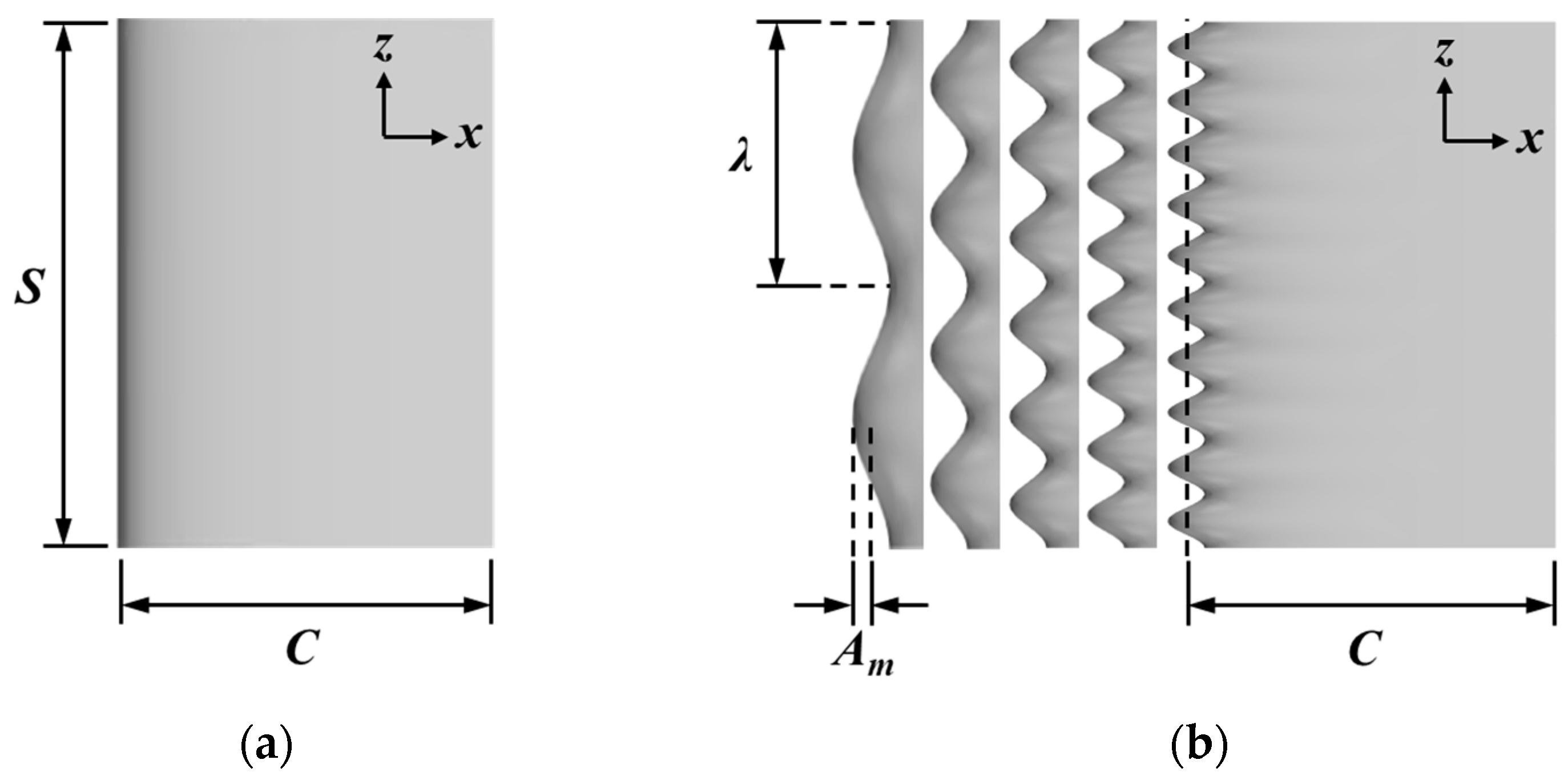
2.1. Definition of Geometry

Figure 1 displays the geometries of and design parameters of the smooth and the wavy wings. The sinusoidal variation along the spanwise direction is applied to construct the leading edge of the wavy wings.

$$C\left(z\right)=C+acos\left(\frac{2\pi z}{\lambda }\right)$$

(1)

where C(z) denotes the local chord length of the profile, $C$ is the mean chord length, a is the wavy amplitude, and $\lambda$ is the wavelength. In this study, the amplitude ($A_m$) and wave number ($W_n$) of the wavy leading edge are considered at 0.0125C, 0.0250C, 0.0375C, 0.0500C and $S$/2, $S$/4, $S$/6, $S$/8, $S$/10, where $S$ is the wing span. The aspect ratio ($AR$) of the wing and the ratio of span are defined as $AR$ = $S$/$C$. The range of the aspect ratio and angle of attack ($\alpha$) are 1.0, 1.5, 2.0, 2.5, 3.0 and 0, 5, 10, 15, 20, 25, 30. Finally, a total of 735 wings including 35 smooth wings and 700 wavy wings were considered.

2.2. Numerical Methods

In this study, the software STAR CCM+ [36] is used to simulate a three-dimensional problem. To simplify the problem, the assumption is made that the flow is steady, incompressible, viscous, and turbulent. Turbulence modelling is carried out by the Reynolds averaging procedure. The governing equations in Cartesian tensor form are written as following continuity, Navier–Stokes, and energy equations in Equations (2), (3), and (4), respectively:

$$\frac{\partial \rho }{\partial t}+\frac{\partial }{{\partial x}_i}\left(\rho u_i\right)=0$$

(2)

$$\frac{\partial }{\partial t}\left(\rho u_i\right)+\frac{\partial }{\partial x_j}\left(\rho u_i{u}_j\right)=-\frac{\partial p}{{\partial x}_i}+\frac{\partial }{{\partial x}_j}\left[\mu \frac{{\partial u}_i}{{\partial x}_j}-\rho \overline{u_i^{\prime }{u}_j^{\prime }}\right]$$

(3)

$$\frac{\partial }{\partial t}\left(\rho T\right)+\frac{\partial }{\partial x_i}\left(\rho u_{i}T\right)=\frac{\partial }{\partial x_i}\left(\frac{k}{c_p}\frac{\partial T}{\partial x_i}-\rho \overline{u_i^{\prime }{T}^{\prime }}\right)$$

(4)

where Cartesian coordinates $x_i$, velocity components $u_i$, density $\rho$, viscosity $\mu$, and pressure $p$, temperature $T$, thermal conductivity $k$, and specific heat capacity $c_p$ are considered. The Reynolds stress term $-\rho \overline{u_i^{\prime }{u}_j^{\prime }}$ and the heat flux of $-\rho \overline{u_i^{\prime }{T}^{\prime }}$ in Equations (3) and (4) are closed using the SST k-ω model. This model is particularly effective in solving a wide range of flow problems, including adverse pressure gradient flows and airfoil flows, and can accurately and reliably solve both near-wall and far-field.

The SIMPLE algorithm and the finite volume method are adopted to the governing equations. The second order scheme is used for spatial discretization. The present simulations use a convergence criterion of 10⁻⁶. For more implementation details, refer to the STAR CCM+ [36] manuals.

Figure 2 shows the boundary conditions and computational domain in the fixed Cartesian coordinate system (x, y, z) based on the origin at the end of the wing tip. The direction of the inflow in the inlet is aligned in the $x$-axis. The domain sizes are allocated to 15$C$ and 10$C$ for the length and the height, respectively. The geometry and dimensions of the numerical model used in this study are those of Kim et al. [5].

The wing surface is subject to a no-slip boundary condition, while the symmetry condition is applied in the far-field boundary. The inflow imposes a uniform flow with the free stream velocity. The outflow receives the convective condition. The wing shape corresponds to the NACA 0020, which has a 1.5$C$ span. The Reynolds number is 1,000,000. The angles of attack vary from 0 to 40.

The typical grid distribution close to the wavy wing is displayed in Figure 3. The minimum grid spacing on the smooth and wavy wing surfaces is about 2 $\times$ 10⁻⁵, which corresponds to a wall unit of $y^{+}$ = 1. The grid spacing becomes gradually coarser as the distance separates from the wing surface. The total number of grids is about 2.6 million.

To validate the accuracy of the current numerical method, a comparison was made with the experimental results from Molland and Turnock [37] and the study conducted by Kim et al. [5]. A comparison was carried out for both a smooth wing and a symmetric wavy wing with an $AR$ of 1.5 at $Re$ of 1,000,000.

In the smooth wing, the present force coefficients are compared with the experimental data from Molland and Turnock [37] up to the post stall. Figure 4a illustrates that the present force coefficients align well with the experimental results from Molland and Turnock [37]. Furthermore, in the wavy wing with an $AR$ = 1.5, $A_m$ = 0.0250, and $W_n$ = $S$/4, the present force coefficients are compared with the numerical results of Kim et al. [5]. Figure 4b demonstrates that the force coefficient from the present study closely matches the findings of Kim et al. [5], as shown in Figure 4b.

The comparisons with experimental data serve to validate the credibility of the present numerical method by showcasing the agreement between the force coefficients obtained in the current study and those obtained through experimental and numerical investigations conducted by Molland and Turnock [37] and Kim et al. [5].

2.3. Dataset of Deep Learning

In this study, three-dimensional wings with various geometric parameters are used as input data for deep learning. A total of 735 cases are considered for the dataset. The training and testing are performed by using 80% and 20% of the dataset, respectively.

The input data consist of three coordinates: $x$, $y$, and $z$. These coordinates were defined based on the circumferential and spanwise directions on the surface of wing, as illustrated in Figure 5. The number of the spanwise coordinates is 64, and also the same number of coordinates, 64, is allocated along the circumferential direction. Therefore, for each individual wing, the total number of coordinates is 4096 $\times$ 3, as depicted in Figure 5.

2.4. CNN and ED Model

The present study is conceptually based on the supervised machine learning technique as one of classifications of machine learning techniques. The algorithm of the supervised machine learning technique is trained by utilizing the labeled inputs to distill the underlying features in the data. The present study will develop CNN and ED models. These deep learning models will predict the flow and thermal characteristics corresponding to input data. Details about the utilized CNN and ED models are given below.

The CNN is considered as a representative deep learning model. LeCun et al. [38] first proposed that enhancing the convolutional layer plays a role in extracting the features of input data through operations with various input data and various filters.

Figure 6 presents typical architectures of the layers of the CNN model and ED model. The CNN and ED models have layer architectures to form an algorithm. Both deep learning models have the same layers: the convolutional layer, fully connected layer, and pooling layer. These layers are called hyperparameters, which will be discussed and evaluated for their effect on prediction later.

Also, the CNN and ED architectures are divided into classification and feature extraction, as plotted in Figure 6. There is the convolution layer and pooling layer. Two fully connected layers are in the classification. The role of the two fully connected layers is for classification of the images. The images are classified by one-dimensional flatten array. One-dimensional flatten array is achieved by converting the previous pooled and convolved layers with two-dimensional array.

Additionally, in Figure 6b, the architecture incorporates the input of geometry parameters, namely $AR$, $W_n$, $A_m$, and $\alpha$, into the fully connected layer. These parameters provide crucial information to the ED model, allowing it to account for the specific geometric characteristics and operating conditions of the wing.

3. Results and Discussion

3.1. Training, Architecture, and Parameters

The training processes for ED and CNN models can correspond to the optimization procedure. The training processes for both models can be achieved by minimizing the mean square error (MSE). Mainly, ADAM [39] and the backpropagation algorithm [40,41] are used for the training processes.

The training process of both deep learning models aims at minimizing the loss function. The loss function is realized by the MSE. The difference between the prediction results obtained by the deep learning models and the true ones from the CFD results define the present MSE in Equation (5):

$$\mathrm{M}\mathrm{S}\mathrm{E}=\frac{1}{N}\sum _{i=1}^N{\left(Prediction-True\right)}^2$$

(5)

where $Prediction$ and $True$ correspond to the output obtained by the deep learning models and the data from the CFD results, respectively. $N$ is the total data point number. The output features are normalized and finally are rearranged between −1 and 1. In other ways, the input images as the pixel values are presented between 0 and 1 without the normalization process.

The selection of pooling, fully connected, and convolutional layers can be tuned according to the problem’s complexity. Consequently, various configurations of the CNN model can be accomplished by changing and combining the numbers of the fully connected and convolution layers, as shown in

Table 1. Parameters for CNN architecture.

CNN Architecture	Convolution Layers	Fully Connected Layers
CNN-1C2F	1	2
CNN-3C2F	3	2
CNN-5C2F	5	2
CNN-3C4F	3	4
CNN-3C6F	3	6

.

The layers of 1, 3, and 5 are adopted as the numbers of the convolution layer in Table 1. Additionally, the layers of 2, 4, and 6 are used to set the fully connected layers. Finally, these different fully connected and convolution layers are combined to construct the CNN architectures which are named, as presented in Table 1, where C is the convolution layer and F is the fully connected and convolution layer. Figure 6a shows the constructed CNN architectures.

First, the dependence of the training of the CNN model on the number of the convolution layers is evaluated for the fixed fully connected layer numbers of 2. The constructed architectures of CNN models are named as CNN-1C2F, CNN-3C2F, and CNN-5C2F, as shown in Table 1, which are considered to investigate the effect of the convolutional layer number on the convergence of the error.

Figure 7 presents the convergence histories of the MSE for different CNN architectures. The convergence histories of the MSE for the three convolutional layers demonstrates similarities in their convergence, as shown in Figure 7. Among these, 3C2F shows the relatively lowest MSE. Thus, 3C is chosen to assess the effect of the number of fully connected layers on the error. The 2, 4, and 6 layers are used for the number of fully connected layers. Resultingly, CNN-3C2F, CNN-3C4F, and CNN-3C6F are tested and, finally, show slight differences in convergence, as shown in Figure 7. As shown in Figure 7, the values of the MSE do not show a significant change before 1000 epochs. As a result, CNN-3C4F is adopted to predict the force and heat transfer coefficient for the smooth and wavy wings.

Following the CNN model, the ED model is also examined for the dependence of the MSE on the convolution and fully connected layer numbers. The combinations of the convolutional and fully connected layer numbers are used to design various ED architectures. The 1, 3, and 5 layers are used for the convolution layer numbers. The 3, 4, and 5 layers are adopted for the fully connected layer numbers. Specific combinations of ED architectures are provided in

Table 2. Parameters for ED architecture.

ED Architecture	Convolution Layers & Convolutional Transpose Layers	Fully Connected Layers
ED-1C3F	1	3
ED-3C3F	3	3
ED-5C3F	5	3
ED-3C4F	3	4
ED-3C5F	3	5

. These ED architectures are plotted in Figure 6b. Therefore, there are a total of five ED architectures: ED-1C3F, ED-3C3F, ED-5C3F, ED3C4F, and ED-3C5F.

In the same procedure as the CNN model, the error convergence of the ED model is also evaluated. Figure 8 presents the convergence histories of the MSE for five different ED architectures. As a result, the convolution and transposed convolution layers of ED-1C3F, ED-3C3F, and ED-5C3F are tested to discover their effects on the convergence of the MSE. There is a negligible difference between different layers in the MSE convergence histories, as clearly identified in Figure 8. Therefore, ED-3C3F with the medium layer number in the three ED architectures is adopted to evaluate the number of fully connected layers by using 3, 4, 5. As a result, three fully connected layers of ED-3C3F, ED-3C4F, and ED-3C5F result in minor differences in MSE convergence. Also, the evaluated ED architectures give almost the same saturation of the MSE. Finally, ED-3C5F is chosen to predict the flow and thermal fields.

3.2. Prediction of Force Coefficient and Nusselt Number

The samples of the 147 wavy wings are used for testing the trained CNN model. Testing the trained CNN model is performed to assess the accuracy of the prediction. $C_L/C_D$ and $Nu$ are predicted for the inputs of the $x$, $y$, and $z$ coordinates on the surface of the wavy wings. $C_L/C_D$ and $Nu$ are commonly used to assess the aerodynamic performance and the thermal efficiency of the wing, respectively. The prediction results achieved by the CNN model are exhibited as scatter plots for $C_L/C_D$ and $Nu$, with true calculated by CFD, as shown in Figure 9. Most of the predicted $C_L/C_D$ and $Nu$ are clustered in the vicinity of the 45-degree line, as shown in Figure 9a and 9b, respectively. This clustering indicates that the predicted $C_L/C_D$ and $Nu$ from the CNN model developed in present study are similar to the true obtained by CFD.

3.3. Prediction of Flow and Thermal Fields

In order to examine the performance of the developed ED model to predict the flow and thermal fields on the surface of wavy wings, an arbitrary four wavy wings were selected. As a result, the four cases for various areas such as case 1 ($\alpha$ = 30°, $A_m$ = 0.0125, $W_n$ = 2, $AR$ = 1.0), case 2 ($\alpha$ = 20°, $A_m$ = 0.0125, $W_n$ = 2, $AR$ = 2.0), case 3 ($\alpha$ = 10°, $A_m$= 0.0125, $W_n$ = 8, $AR$ = 1.5), and case 4 ($\alpha$ = 10°, $A_m$ = 0.0375, $W_n$ = 8, $AR$ = 2.5) are utilized to examine the predictive ability of the ED model. The four cases have a wide range of $C_L/C_D$ from about 2 to 15, as shown in Figure 9a.

Figure 10 and Figure 11 present the contours of the pressure coefficient and the limiting streamlines on the upper surface of the wavy wing, respectively. Thus, the comparisons of the predicted and true flow fields are available. Also, the distributions of errors between the prediction and the true are presented, which measure the accuracy of the developed ED model for predicting each field. In the predicted results, there is an oscillation of the contour boundary relative to the true, but it shows a very similar pressure distribution overall, irrespective of the geometric parameters defining the wavy wing.

A relatively large difference between the prediction and true is observed near the leading edge and root of the wing, where the local pressure exhibits sharp gradients, as shown in Figure 10a–c. In contrast, the results are remarkably consistent between the prediction and true near the trailing edge, where the pressure gradients are relatively low, and near the wingtip, where the characteristic features of the tip vortex are clearly visible, as shown in Figure 10. As the wave amplitude and wave number increase, the pressure distribution is very well predicted near the crest and trough of the leading edge, where the shape of the wave wing is more prominent. Additionally, the pressure distribution in the vicinity of the tip vortex is consistently predicted in all cases.

The developed ED model similarly predicts the limiting streamlines on the upper of wavy wing compared to the true, irrespective of the wave parameters, as identified in Figure 11. According to these wave geometric parameters, the characteristics of the limiting streamlines of true were well predicted by the ED model. In Figure 11a, the flow separates from the leading edge. Also, in Figure 11b, the limiting streamlines exhibit a helical nature, leading to convergence lines and return flow from the trailing edge. Figure 11c,d display flow patterns that closely resemble those of a smooth wing, with a small vortex appearing locally near the trailing edge due to the wave effect. These patterns of limiting streamlines correspond to the pressure distribution, as previously shown in Figure 10c,d. Furthermore, these patterns of limiting streamlines are consistent with the results of previous studies [5,42,43]. As a result, regardless of wave parameters, the characteristics of limiting streamlines such as flow separates, helical nature, and small vortex were almost similarly well predicted, as shown in Figure 11.

Figure 12 shows the contours of the Nusselt number on the upper surfaces of the wavy wings. Thus, comparisons of the predicted and true thermal fields can be performed. Also, the distributions of errors between the prediction and true are presented, which measures the accuracy of the developed ED model for predicting the thermal field. The forced convection over the smooth and wavy wings is governed by the flow. Therefore, these forced convections can be explained by the flow fields.

The prediction results in Figure 12 exhibit oscillations at the contour boundary, similar to the prediction of the pressure distribution in Figure 10. However, the prediction is similar to true across the board. Figure 12 shows a similar error distribution to that shown in Figure 10a,c. A relatively large difference is exhibited between the prediction and true near the leading edge and the root of wing, as shown in Figure 12a–c. In particular, the Nusselt number distribution is well predicted near the trailing edge of the wing, mirroring the characteristics of the limiting streamline shown in Figure 11c,d, as shown in Figure 12c,d. The Nusselt distribution on the surface of wing, as shown in Figure 12, exhibits a similar trend to that shown previously in Figure 10 and Figure 11. As a result, higher accuracy is observed in cases where the characteristics of the wave are more pronounced.

Koziel et al. [44] compared the computational performances of the proposed approaches. The computational performance of the methods used in this study is compared with reference to their paper.

Table 3. Performance comparison between CFD and the proposed methods (CNN&ED) in terms of the computational cost of predicting aerodynamic and thermal performance.

Method	Simulation Time
CFD	30 min
CNN	1 s
ED	1.5 s

shows a performance comparison between CFD and the proposed methods in terms of the computational cost of predicting aerodynamic and thermal performances. The computation equipment used was an Intel Xeon Gold 6240 CPU 2.60GHz 36 core processor and NVIDIA GeForce RTX 3090.

In the case of using CFD, there is a slight difference depending on the convergence, but it takes about 30 min per 1 case. In the case of the CNN and ED models, it takes about 4 h to train. When using a trained CNN and ED model, it takes about 1~1.5 s per 1 case. As a result, the proposed methods provide a highly efficient computational time for the prediction of aerodynamic and thermal performances.

4. Conclusions

The present study established CNN and ED models to predict the characteristics of flow and heat transfer on the surface of a three-dimensional wavy wing with a wide range of parameters, including aspect ratio, wave amplitude, wave number, and angle of attack. The presently established CNN model was utilized to predict aerodynamic and heat transfer coefficients for smooth and wavy wings. Another established ED model was utilized to predict the distributions of the pressure coefficient, limiting streamlines, and Nusselt number on the surface of a wing. The dataset was constructed through CFD. To validate the accuracy of the numerical methods of CFD, a comparison of the CFD results was made with the experimental results.

The architectures of the CNN and ED models were tested by changing various hyperparameters of the convolution layer, the transpose convolution layer, and the fully connected layer. These architectures were evaluated by the MSE convergence histories, achieving proper hyperparameters. The predicted aerodynamic coefficients and Nusselt number for smooth and wavy wings using the CNN were compared to the true using a scatter plot; it showed a very similar result.

The distributions of the pressure coefficient, limiting streamlines, and Nusselt number on the surfaces of the smooth and wavy wings were well predicted using the ED model when compared to the corresponding true results. The true results obtained by CFD showed that as the angle of attack increased, the symmetric wavy wings formed helical vortical structures on the surface, which had a positive effect on the aerodynamic performance. These complex helical vortical structures were also captured by the present ED model. The predicted limiting streamlines revealed a separation delay due to the effect of the wavy formation.

However, the shapes of these helical structures in the ED model were slightly different. In addition, near the leading and trailing edges, the differences between the predicted and true results appeared. These regions were exposed to very sharp velocity gradients. Thus, the ED model needed a larger dataset, which was achieved using more resolved grid systems for CFD.

Consequently, it is expected that the presently established CNN model performs a parametric study to discover the ideal conditions to provide efficient aerodynamic and thermal performances. Then, the presently established ED model predicts the reasonable flow and thermal characteristics to support the physical interpretation for variations in the aerodynamic and heat transfer coefficients obtained by the present CNN model.

In general, the deep learning model is strongly dependent on the dataset. Thus, the dataset should be set up according the application, which is still very expensive.

The proposed methods will be used as a method of predicting the aerodynamic and thermal performance of three-dimensional shapes in real-world applications. In addition, it is expected to be a more efficient method than existing methods using systematic parameters based on a high-quality database.