Abstract
In this work, we present a grid study oriented to capture 3D flow simulations around smooth and wrinkled cylinders that could have practical applications in various engineering areas. The study considers three Reynolds numbers, namely, a benchmark Re and two orders of magnitude above and below it. The main contributions of the paper relate to the optimization of the computational mesh for the spanwise direction of the wind flow that results from the computational-mathematical framework employed, in addition to a novel visualization technique that unfolds features in the recording data that could otherwise be hidden when using traditional plots. We compare our benchmark results with those reported by other authors to conclude that the intermediate resolution grids employed with the widest spanwise provide acceptable results. Furthermore, the new visualization technique offers significant advantages compared to traditional pressure maps, regarding clarity for observing and interpreting local flow disturbances, making variations with Re clearer, and by enabling the detection of asymmetries.
1. Introduction
Flow around square cylinders at a Reynolds number (Re) of around is widely studied given its relevance to characterize fluid performance in the subcritical range, and its adaptability to industrial and energy problems. Its main applications relate to ocean engineering–energy production [1,2], drag reduction [1,3,4], and the aerodynamic optimization of squared-rectangular vehicles [5,6,7].
Most of these developments involve computational fluid dynamics (CFD) simulations oriented to improve passive control, e.g., for designing geometries that control the flow or through modifications to the cylinder’s shape. Here, a trade-off arises for maximizing the accuracy of the results at the lowest computational cost, which leads to a structural and refinement meshing problem given the type and extent of the modifications required.
As a fluid dynamics problem, computational simulations must be validated with experimental results. Some published experimental data can be found in [8], corresponding to a smooth-squared cylinder at Re . Likewise, Ref. [9] performed wind-tunnel measurements using rectangular cylinders with different aspect ratios and inclination angles, covering Re , including Re . In addition, Ref. [10] worked with different types of cylinders, including the square case at Re , while Ref. [11] undertook experiments and simulations at Re and . Most of these works focused on the effects of turbulence near the wake and measurement of the corresponding force coefficients.
The flow around regular objects is relevant for engineering applications as it helps to understand wake formation and the (time-averaged) loads around buildings. For this reason the visualization of the flow around a square-section cylinder has received considerable attention, for example via detailed laser Doppler velocimetry (LDV) studies by [12] at Re and [8] at the Reynolds number mentioned above, both at zero incidence. The authors of [13] extended studies of a similar kind considering non-zero incidence, i.e., considering the orientation of the rectangle, by means of particle image velocimetry techniques (PIV) at Re , , and . These research developments presented classical velocity contours, vector fields, or streamlines. In this sense, our proposal offers an alternative visualization tool to characterize related phenomena that could, for instance, complement the implementation studies presented by [14]. These authors studied numerically the aerodynamic characteristics of a rounded-corner square cylinder for Re , in addition to other engineering key problems, like those presented by [15,16], who studied experimentally the aerodynamic effects of surface-mounted ribs on square-section high-rise buildings.
Current practice for the reproduction of smooth-squared and low-modified cylinder cases is the building of computational arrays with structured meshes, adding non-uniformity near the walls of the cylinders. Given the symmetry of the object, the majority of these works capture 2D-flow effects, disregarding other effects taking place in the spanwise direction, but using large amounts of cells to try and accurately reproduce the experimental results. In this regard, the Re is of special interest as it relates to one of the two benchmark problems recognized by the European Research Community on Flow, Turbulence and Combustion (ERCOFTAC) in 1996 [17].
Some numerical studies and schemes used to scrutinize the benchmark address drag reduction by modification of the front or rear side of the bluff body with very large eddy simulations (VLES) [1], the reproduction of flow with LES, and spectral vanishing viscosity methods covering a near-wall region [11]. These examples include three types of models, namely, 2D unsteady Reynolds-averaged simulations (URANS), 3D LES/RAS, and 3D improved delayed detached eddy simulations (IDDES) [18]. Moreover, the following techniques provide added elements to the discussion: the Spalart–Allmaras model and DES [19], LES and the Smagorinsky model [20,21,22], VLES [23], and partially averaged Navier–Stokes (PANS) simulations [24,25].
It is worth mentioning that all of the works cited above used structured computational arrays, which work well when the cylinder (object) has a simple shape that can be built up with structured-meshing elements that are available in commercial software. Yet, meshing complex geometry using structured meshes is particularly difficult. Indeed, the addition of a boundary layer or a certain non-uniformity near the object requires much extra refinement and could become hard to implement with structured meshes alone [26]. Thus, when dealing with complex geometries, unstructured meshes become highly attractive to fit the object’s shape without affecting the quality and accuracy of the results. To the best of our knowledge, the only two reported works that have used a non-structured mesh are [25,27]. Ref. [25] developed the meshing with ANSYS ICEM, to then perform their simulations in OpenFOAM. The size of their computational array is similar to those of the abovementioned studies and has uniform extrusion in the spanwise direction, inflation layers near the walls, and non-uniformity moving away from the object, leading to around cells. In turn, Ref. [27] designed their simulations in a similar way to our approach in the present study: the object was constructed in FreeCAD and applied an unstructured mesh in OpenFOAM, but targeting a different Reynolds number, that is Re .
In this work, we simulated the flow around a square cylinder at Re , Re , and Re , by carrying out 3D-delayed detached eddy simulations (DDES) with the Spalart–Allmaras model as the closer. For the intermediate Re (benchmark problem), five unstructured computational arrays were tested systematically by narrowing down their depth in the spanwise direction (leading to a change in cell number) while observing the lateral limits of the domain. We used the SnappyHexMesh tool embedded in OpenFOAM (version 2012) [28], which is a free, open source CFD software Author Reply: (version v2012, released by OpenCFD Ltd.—ESI Group, mainly located in Bracknell, England) that allows simulating fluid–structure interactions. This software was used by some of the works mentioned above but using structured meshes, specifically by [1,23,24]. Once having optimized the computational array, our study puts forward two innovations:
- 1.
- A detailed description of the benchmark case, providing explicit characteristics of the mathematical-computational framework that optimizes the computational resources to produce comparable 3D flow disturbances with experiments and other simulations.
- 2.
- A polar visualization of time-averaged flow variables in concentric shells surrounding the object, leading to a novel classification of the flow patterns resulting from the proposed visualization. Moreover, a proper extension of the benchmark to different Re and to non-smooth cylinders is suggested.
The paper is organized as follows: All the considerations relating to the design of our computational model are introduced in Section 2.1 and Section 2.2. Section 2.3 presents the grid convergence study and includes the preliminary results for the optimization of the grid. Then, we discuss the results with respect to our first contribution in Section 3.1, and cover the second in Section 3.2. We extend our discussion on the proposed visualization technique in Section 4. Final remarks are presented in Section 5. Except where otherwise specified, we use the terms square, cylinder, and object, without distinction throughout our study case, as well as grid and mesh.
2. Computational-Mathematical Model
2.1. Governing Equations and Numerical Method
The unsteady numerical simulations of the incompressible flow were performed by embedding a delayed detached eddy simulations (DDES) solver. The DDES model was merged with the Spalart–Allmaras (SA) model [29,30], which is based on the modified turbulent viscosity :
In Equation (1), is the density of the fluid, refers to the shear stress, the turbulent viscosity () is recovered by , with , and is the length scale defined by,
The RAS scale is , with the distance from the analyzed cell to the closest solid wall; the LES scale is , with the MIN function as a low Reynolds number correction function and as a length proportional to the local grid spacing , where is a constant. In this way, Equation (2) allows varying the length scale in Equation (1) depending on the proximity to the closest solid wall, from a full RAS model when it is far apart, to a full LES model when it is sensibly close. The transition between scales is also softened by the delay function
where is a MIN function depending on the velocity vector of the fluid , its viscosity and the distance , so that . This construction was fully implemented in a cube-root volume formulation by the function cubeRootVol. The coefficients , , , , , , , and functions , , and the rest of the implicit parameters of the model were set to default values [31,32].
Regarding the method of solution, OpenFOAM is designed to work with unstructured meshes, utilizing the finite volume method (FVM) to construct a way of integrating the Navier–Stokes equations over a 3D control volume V, leading to the general scalar transport equation for our problem as the conservative form
with source for each property (components of velocity and mass). Equation (4) is then discretized by the divergence theorem to produce a system of algebraic equations of the form to be solved, where coefficient matrix, vector of variables, and source vector. For our numerical simulations, the discretization process was performed by using a conditionally stable second-order implicit-backward for time schemes, Gauss linear for gradient schemes, Gauss linear limited for divergence and Laplacian schemes, and linear interpolation to transform the cell-center quantities to face centers. Although it is worth mentioning that investigating the discretization process performed by OpenFOAM is outside the limits of this study, readers with a special interest in step-by-step similar procedures are referred to [14,33,34].
To achieve the above purpose, we implemented the PISO (Pressure Implicit with Splitting of Operators) algorithm, which is a transient incompressible (in OpenFOAM [35]) iterative procedure that splits the operators into an implicit predictor and multiple explicit corrector steps, seeking to obtain close approximations of the exact solution of the difference equations at each time-step, with the accuracy in terms proportional to the powers of the time-step size. Further details of the PISO algorithm are found in [36,37]. In pisoFOAM, pressure is fully implicit, with the coupling of the velocity and pressure equations being handled through the iterations, by evaluating the initial solutions and then correcting them. For this, we delimited a maximum of three corrections without extra-correction for mesh non-orthogonality. In this context, the resulting algebraic equations were solved by different methods: a generalized geometric-algebraic multi-grid (GAMG) solver method for pressure, with a Gauss–Seidel method as a smoother, and a preconditioned pipelined conjugate residuals (PPCR) solver to override solution tolerance for the final pressure, and a symmetric Gauss–Seidel solver for the rest of the variables. These and all other parameters and methods were set according to default values of the motorbike example in OpenFOAM-v2012, see the tutorials [38] for more details (once installed, refer to directory: OpenFOAM/OpenFOAM-v2012/tutorials/incompressible/pisoFoam/LES/).
2.2. Meshing, Initial, and Boundary Conditions
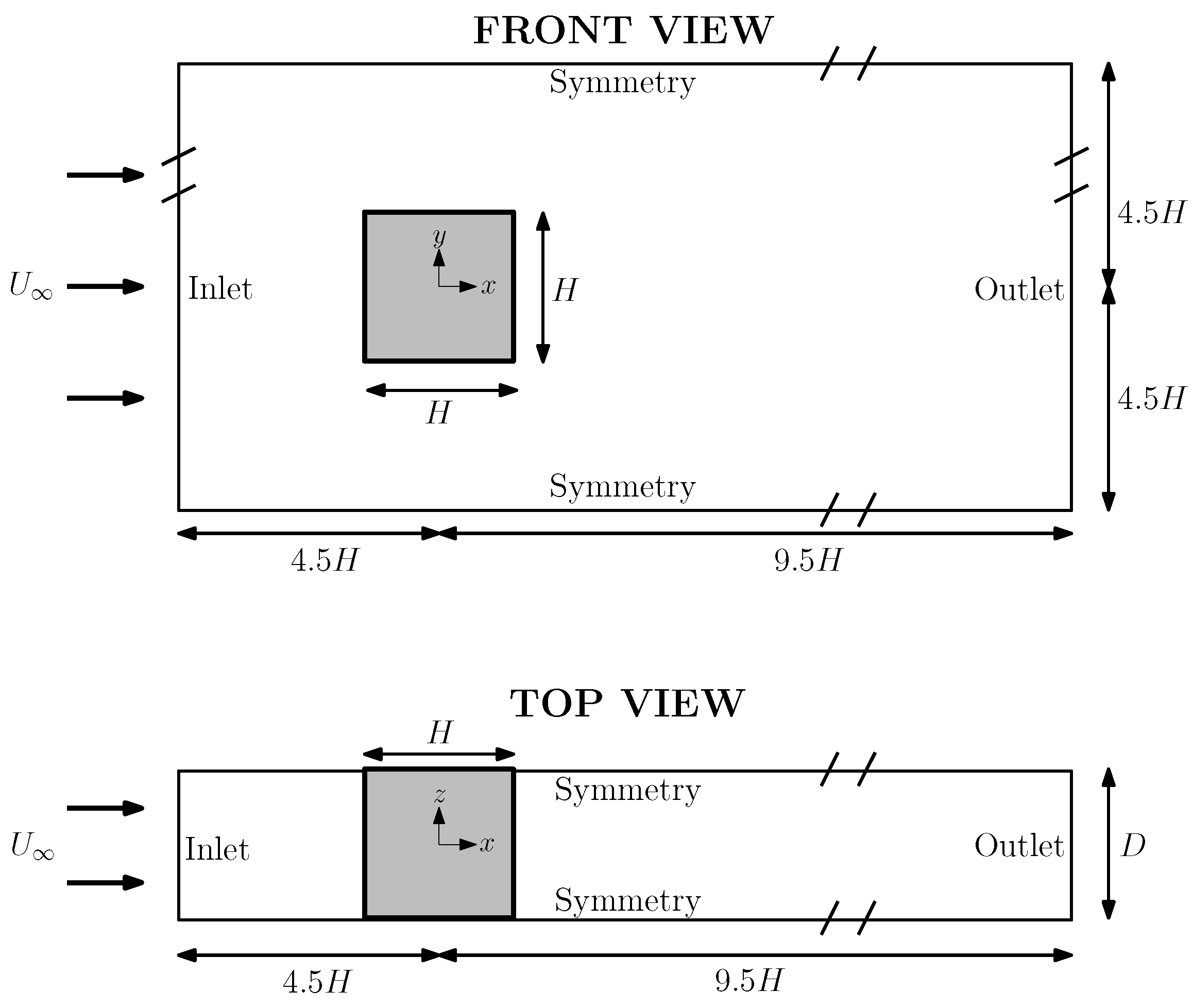
The computational domain is defined in Cartesian coordinates. According to Figure 1, the origin of the system is located at the center of the squared cylinder, characterized by length L, height H, and width D, along the x, y, and z axes, respectively. The main flow aligns with the x-direction and the cylinder traverses the entire domain in the z-direction; thus, H is taken as the characteristic length of the system. We set m and for all the numerical tests; note that the values of D are described in Section 2.3.
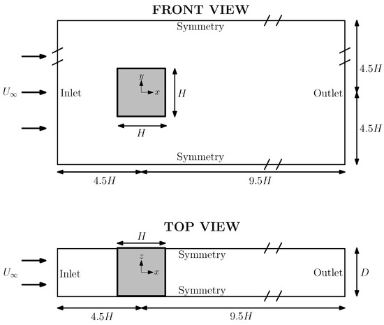
Figure 1.
Schematic representation of the problem showing the selected scales and boundary types for two plane views.
For defining limits of the computational domain, we used three levels of boundary conditions (see Figure 1). Inflow and outflow boundaries were located at and , respectively. In turn, symmetry boundaries were implemented at the rest of the borders of the domain, enclosed within (up and down), and (front and back). Finally, the non-slip boundary was implemented at the walls of the cylinder. The objects (cylinders) were designed in FreeCAD and imported as a STereoLithography (STL) file by means of the surfaceFeatureExtractDict tool of OpenFOAM, extracting the edges of all angles. We used FreeCAD version 0.18, with its latest version being accessible at [39].
The initial and boundary values of the parameters at each boundary and internal fields are shown in Table 1. Re = is obtained by fixing a free stream velocity m/s in the x-direction at the inlet, and considering a kinematic viscosity m2/s, which is defined in the directory constant/transportProperties. In order to reproduce the experimental setup of [8], we define a uniform turbulence intensity % at the inlet, leading to a turbulent energy of m2/s2; it was modeled by the function kqRWall for cells at the cylinder’s wall. In addition, the turbulent kinematic viscosity is calculated at the inlet and outlet boundaries, and modeled at the cylinder by the function nutUSpaldingWall. The modified turbulent viscosity is set to in all the domain, excepting for cells near to the cylinder’s wall in which , as usually suggested [29,40]. Then, the lower () and higher () Re are obtained by modifying the kinematic viscosity by two orders of magnitude, respectively.

Table 1.
Initial and boundary conditions of the parameters and variables of the model. For the internal field the initial condition only applies.
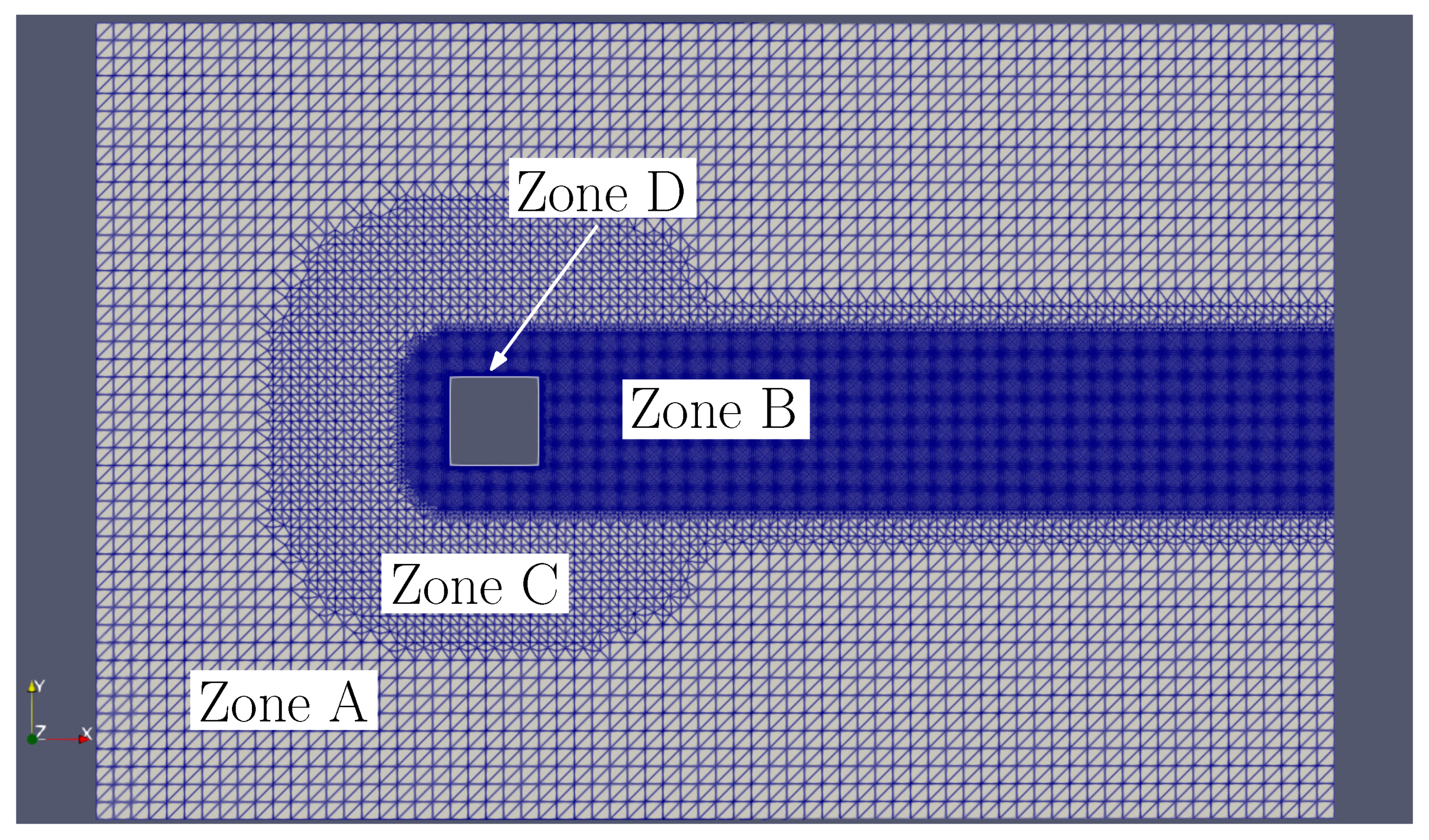
The mesh consists of two uniform-structured grid sections (Zones A and B), one scaled-non-structured grid section (Zone C), and an additional more refined non-structured grid section (Zone D), as shown in Figure 2. Zone A is a coarse grid whose cells consist of quasi-cubes of 1 m3 approximate volume, i.e., per side, with the aim of properly implementing the cube-root volume formulation; the grid is the background of the entire mesh and was defined by the blockMesh tool of OpenFOAM. The rest of the zones were implemented by means of the SnappyHexMesh tool. Zone B is a prismatic-rectangular region defined from to , covering the wake with a refinement level 3. According to the SnappyHexMesh tool, this means that the length of each base cell’s side is divided into parts leading to per side; this would be into () for level 4, and so on. Zone C presents three refinement levels that change with the distance from the cylinder: the maximum refinement level L, depending on each test, was set from the cylinder’s wall to a radial distance of , then, level 3 up to a distance of , and level 1 ( per side) up to . The latter was implemented with the mode distance of the SnappyHexMesh tool. Zone D conforms with the cells defining the STL geometry, in which the surface-wise minimum and maximum refinement level were set to level L.
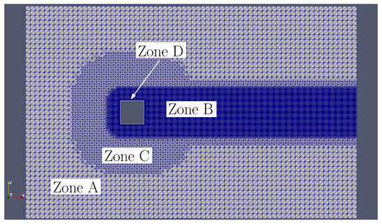
Figure 2.
Section view, in plane x–y, of the four mesh zones of the computational array, showing Zones A–D. Zone D is difficult to see since it delimits the object and has the highest resolution.
When two different refinement levels overlap, the higher resolution prevails. The parameter nCellsBetweenLevels was set to 1 in order to scale the mesh between the different levels using a distance equal to the size of 1 cell of the lower level. All the other parameters for the meshing were set according to the default values of the motorbike example that was mentioned above.
2.3. Grid Convergence Study
To validate our computational-mathematical model at the benchmark Re = , we tested its spatial convergence by mesh arrays with different cell refinements and cylinder depths, looking to identify the most viable mesh that validated the flow while optimizing the computational resources. We considered four resolution levels, from L3 to L6, applied to the three narrowest arrays: D20, D40, and D60. A detailed description of the referred mesh arrays is shown in Table 2 where it can be seen that the total number of cells increases linearly according to the depth of the array. In turn, a change in refinement from L3 to L4 implies an increase of less than 10%, while passing from L4 to L5 leads to an increase of more than 50%, and from L5 to L6 increases the number of cells by almost 400%. This was a first reason to focus our main study on L5. Thus, two meshes with depth D80, D100, and a maximum refinement level of 5 were also included for use once the grid was calibrated for convergence.
Table 2.
Depth of the array and number of cells per refinement level of each mesh. The meshes are named DDLL, where D is the percentage of depth (in terms of H) and L is the maximum level used.
In order to keep the Courant number below 1, the time interval was set to s, s, and s, for meshes with a maximum refinement level of 3, 4, and 5–6, respectively. To standardize the data representation, the graphics and results are dimensionless, e.g., , and .
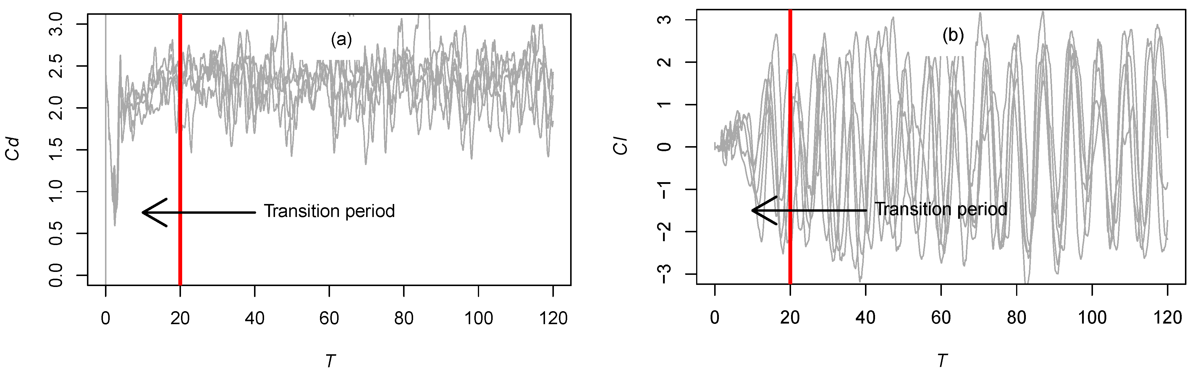
The simulation time of each test was limited to 60 s; however, our analysis excludes data recorded before s to disregard the transition period—according to this, the dimensionless time considered for each simulation becomes units. The start time for data processing is illustrated for drag and lift coefficients in Figure 3. For a clear visualization, only mesh arrays with a maximum refinement level of five are plotted. Beyond the chaotic initial period, large-scale similarities between arrays can be seen in both time series, highlighting the synchronicity shown in from .

Figure 3.
(a) and (b) time series, for mesh arrays with L5 as maximum, tagging the dimensionless time that separates the transition period from the analyzed time.
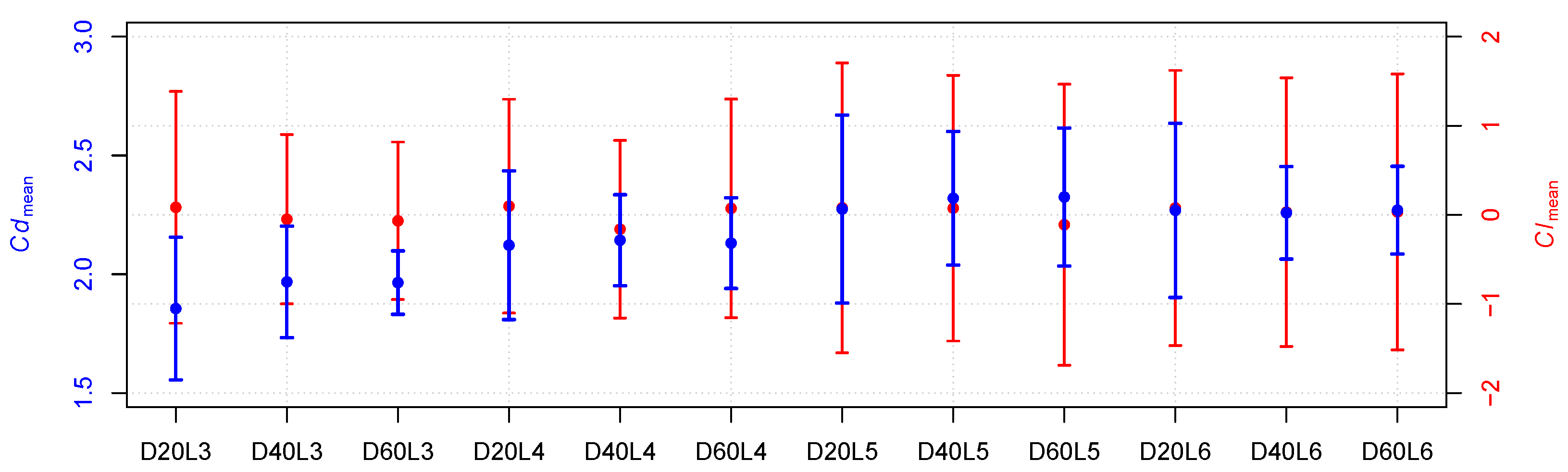
The mean and RMS estimations for both the drag and the lift coefficients are plotted in Figure 4. There it can be seen that the drag coefficients seem to converge at the maximum refinement level. Convergence is reached for the average and for the RMS from the mesh arrays with refinements L5 and L6.
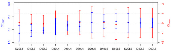
Figure 4.
Time-averaged drag () and lift () coefficient values for different mesh arrays and their standard deviation with error bars.
This also applies for lift, which fluctuates around zero for all meshes.
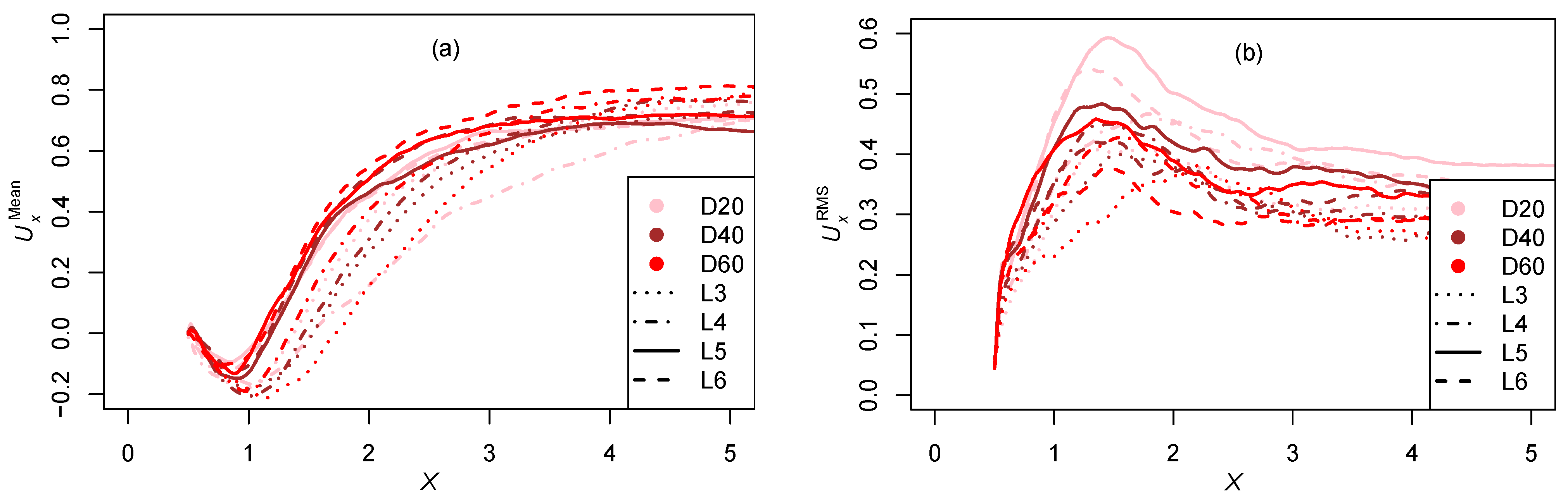
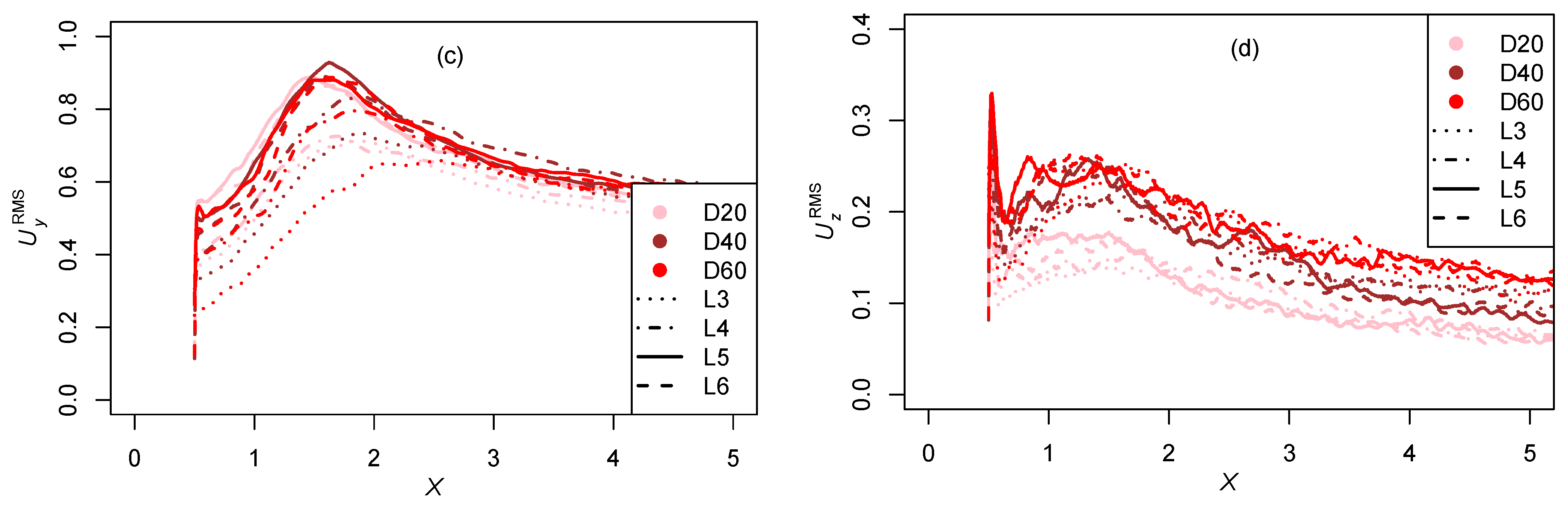
Figure 5 shows changes in the mean streamwise velocity , the root mean square (RMS) of the streamwise , the cross-stream , and the spanwise velocities, recorded between the downstream edge of the cylinder () to . As expected, convergence can be mainly observed in Figure 5a–c, where the dotted and dotted-dashed lines (L3 and L4) differ more from L5 and L6. The narrowness of the mesh seems to have stronger effects in the spanwise direction Figure 5d, where the flow disturbances also converge but to a different curve, depending on the depth of the array. So, it can be deduced that the flow is more restricted along the z-axis for the narrowest arrays, which could cause the lower variations observed. In turn, the RMS of the streamwise direction Figure 5b shows some discrepancies of about dimensionless units between and , when passing from D40L5 and D60L5 to D40L6 and D60L6. Although it is a relatively small difference, we did not find a clear physical-computational cause for this effect, so it could also be associated with narrowness, as suggested by other authors, for example those mentioned in Section 3.1.2.

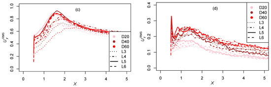
Figure 5.
Perturbed wake along the flow direction in the central line , obtained with meshes with depths D20, D40, D60, and all considered refinement levels (12 meshes in total). In the legend, color refers to the depth of the array, while the line type denotes its maximum level of refinement, so that their addition gives the name of the mesh plotted, in accordance with Table 2. (a) Mean streamwise velocity. (b) RMS streamwise velocity. (c) RMS cross-stream velocity. (d) RMS spanwise velocity.
The above observations lead us to disregard meshes involving D20 and D40, and to further explore D60 together with two wider meshes, D80 and D100. The latter were not considered during the grid convergence study because of limitations in our computational resources (mainly with L6). To perform the tests, we ran simulations in parallel using the scotch method from the decomposeParDict utility of OpenFOAM with 24 subdomains. We used a cluster with Intel® Xeon® CPU E5-2680 v3 at 2.50 GHz with 48 Cores and 131.072 GB RAM, having available 500 GB of storage. All the above settings of the present section apply for both the grid convergence study and the main study.
3. Numerical Results
3.1. Validation with Literature and Meshing Optimization
As the grid was calibrated for convergence, our L5’s computational arrays were ranked according to the computational cost and the accuracy of the results, dismissing those with D20 and D40. At this stage, we compared the results of the former arrays with data reported in the literature for the benchmark. The drag and lift coefficients were targeted and characterized with the respective mean and RMS values. In turn, the wake was analyzed across the near and far zones by scrutinizing the streamwise , cross-stream , and spanwise components of the velocity.
3.1.1. Drag and Lift Coefficients
Table 3 lists the mesh parameters, the estimated force coefficients, and the computational cost, and, whenever possible, compares these with the equivalent values derived from simulations and experimental results reported in the literature. It is worth highlighting that all of our meshes have similar resolution, as expressed in Section 2.2, so that the difference in the number of cells is caused by the depth of the array. Furthermore, our computational arrays seem finer than similar works reported in the literature [1,8,19,22,23,24]; see, for example, the depth and distance from the origin to the input, output, and top/bottom boundaries (columns 2, 4–6 of Table 3). Our arrays are similar to the experimental setup reported by [8] with regards to the input, output, and top/bottom distances, yet smaller than the simulation setups [1,19,22,23,24]. Notably, our largest array (D100L5) is four times smaller in depth than the shortest arrays reported in the literature. This compactness allows reducing the number of cells in comparison with previous simulation setups without loosing resolution.
Table 3.
Force coefficients, CPU time, file size, and some characteristics of our computational arrays compared with previous results reported in the literature. In, Out, and TB refer to the distance from the origin to the Input, Output, and Top/Bottom boundaries. CPU time and file size were measured at the end of the simulation (), following the setup and parameters in Section 2. * The number of cells in [24] is not specified clearly.
The file size of our meshes increases linearly with the depth and the amount of cells of the array, but the CPU time increases non-linearly. The estimated values of are similar across all our meshes. They are also consistent with the corresponding values obtained by [1,22], although [19] reported a value 200% higher. Although we observed a slight increment of , the depth of the array affects neither the nor the results. Moreover, our results are in good agreement with the experimental data, showing relatively small discrepancies of 6–7% that fall within the range encountered in most other simulations. No definitive conclusions can be drawn from the results since we obtained values between 1.47 and 1.71, which slightly overlap the values reported in previous studies, with values of this parameter ranging between 1.03 and 1.5.
3.1.2. Wake Flow Study
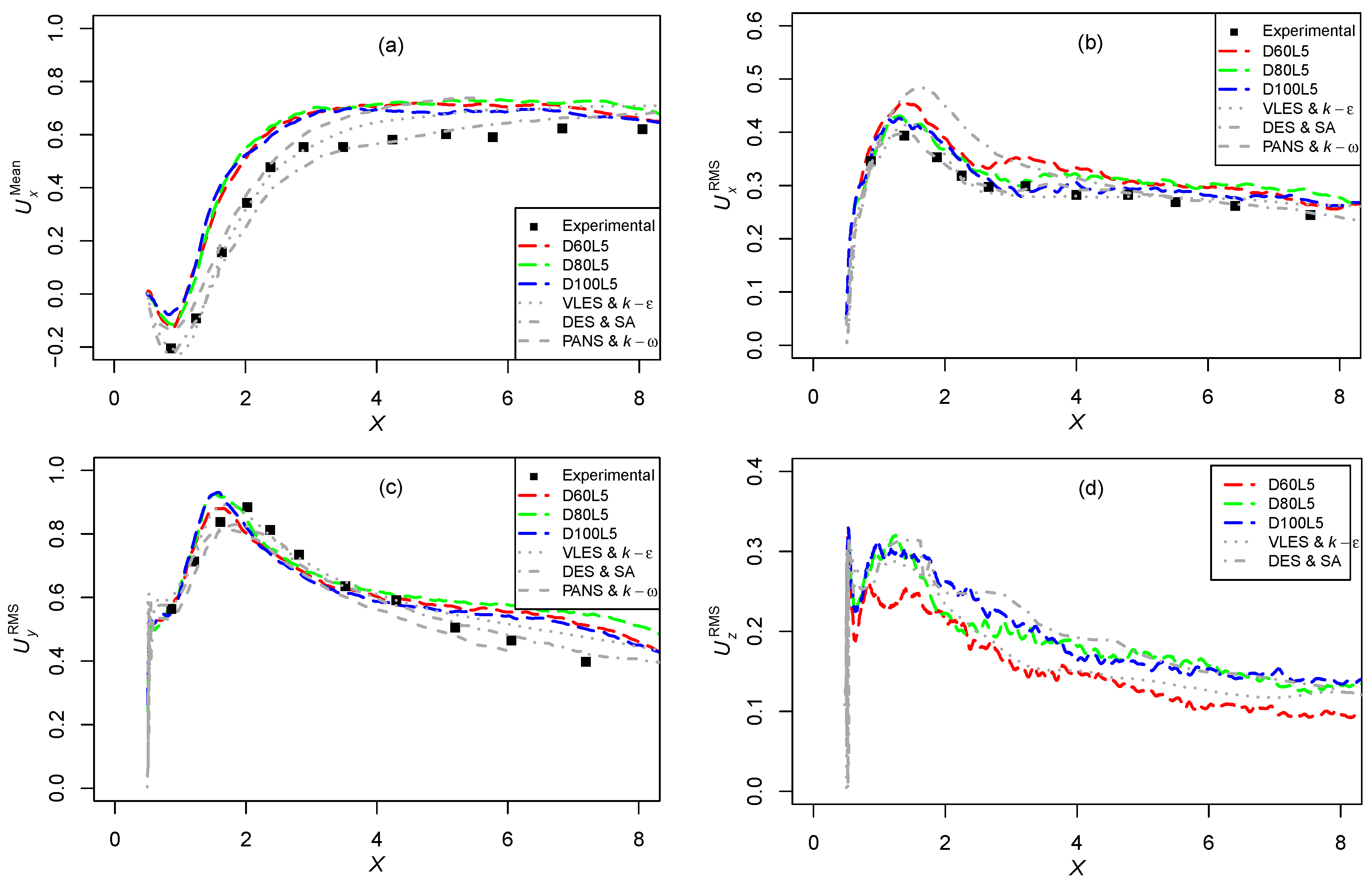
Turbulence was also analyzed along the flow direction (x) in its central line , and in the transverse direction (y) along four separate lines: 1, 2.5, 4, and 6, by referring to the streamwise and cross-stream velocities. The results were compared with the experimental data reported by [8] as well as with some available simulations performed with the PANS & k- model by [24], with the VLES and k- model [1], and by [19], who used a similar approach to that proposed in our work: the DES and SA model, but quadrupling the number of cells of D100L5.
Figure 6 shows the changes in , , , and , recorded between the end of the cylinder () and near the output boundary (). There, we can see that our results capture the general behavior of all the variables qualitatively, although they slightly overpredict the values, Figure 6a, reported in [8], between the domain and . In turn, the VLES [1] and PANS [24] simulations start to diverge from for that variable, whereas the DES and SA scheme proposed by [19] shows differences in the far wake (from ).
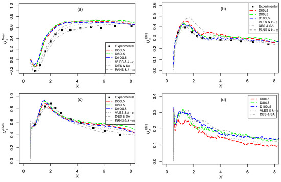
Figure 6.
Perturbed wake along the flow direction in the central line , obtained with meshes with a maximum refinement level of 5. (a) Mean streamwise velocity. (b) RMS streamwise velocity. (c) RMS cross-stream velocity. (d) RMS spanwise velocity.
Furthermore, our results are consistent with the experimental data (mainly with D80L5 and D100L5) for , Figure 6b, in the same order to [1] and close to [24]. In contrast to these, [19] tends to magnify from . For , our simulations and those by [1] reproduce the turbulent effect in the near wake, with a small gap, but are distinguished from the experimental results in , while [19,24] captured disturbances patterns all along the line . Although Lyn (1995) and Chakraborty (2020) reported no values for , the results of D80L5 and D100L5 reproduce the peak observed between –, which reaches and coincides with the results reported by [1,19]. However, the curve obtained by [1] falls quickly from and fits our mesh D60L5, whose behavior could be influenced due to the narrowest configuration of the array.
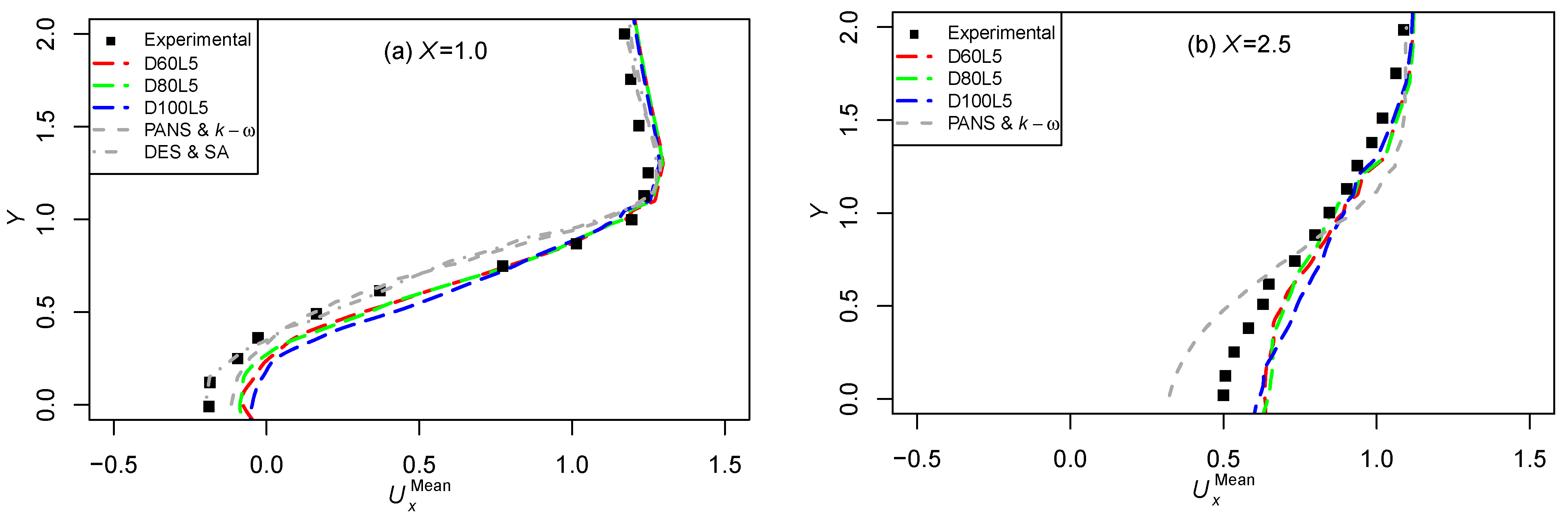
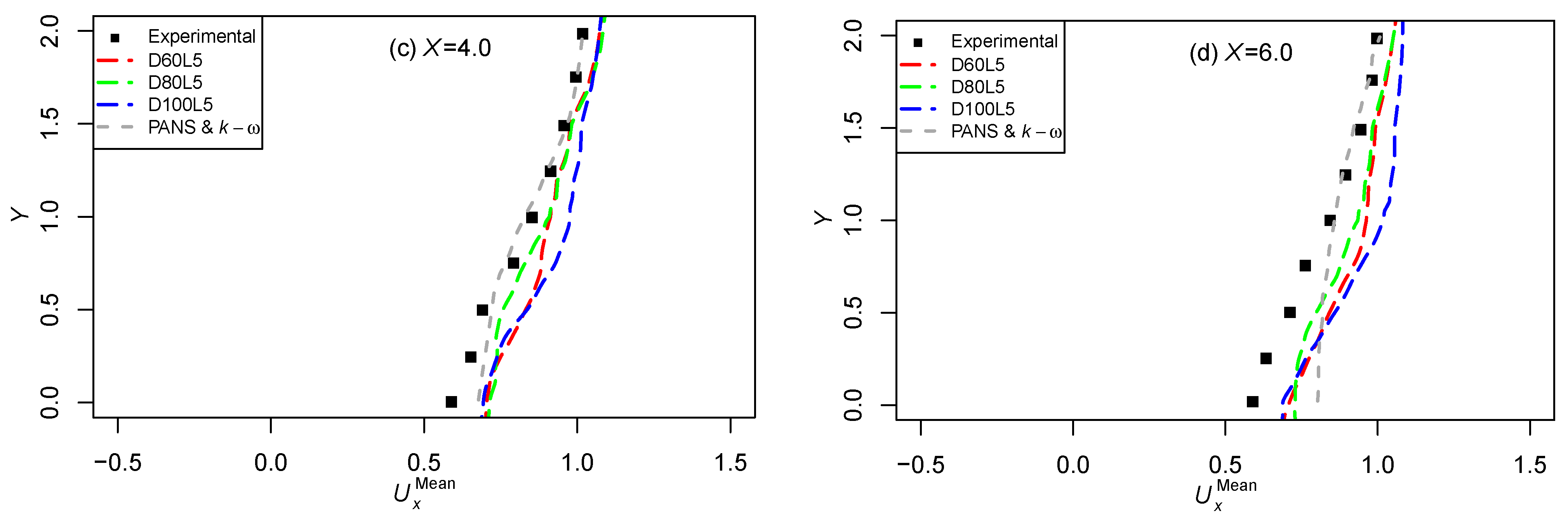
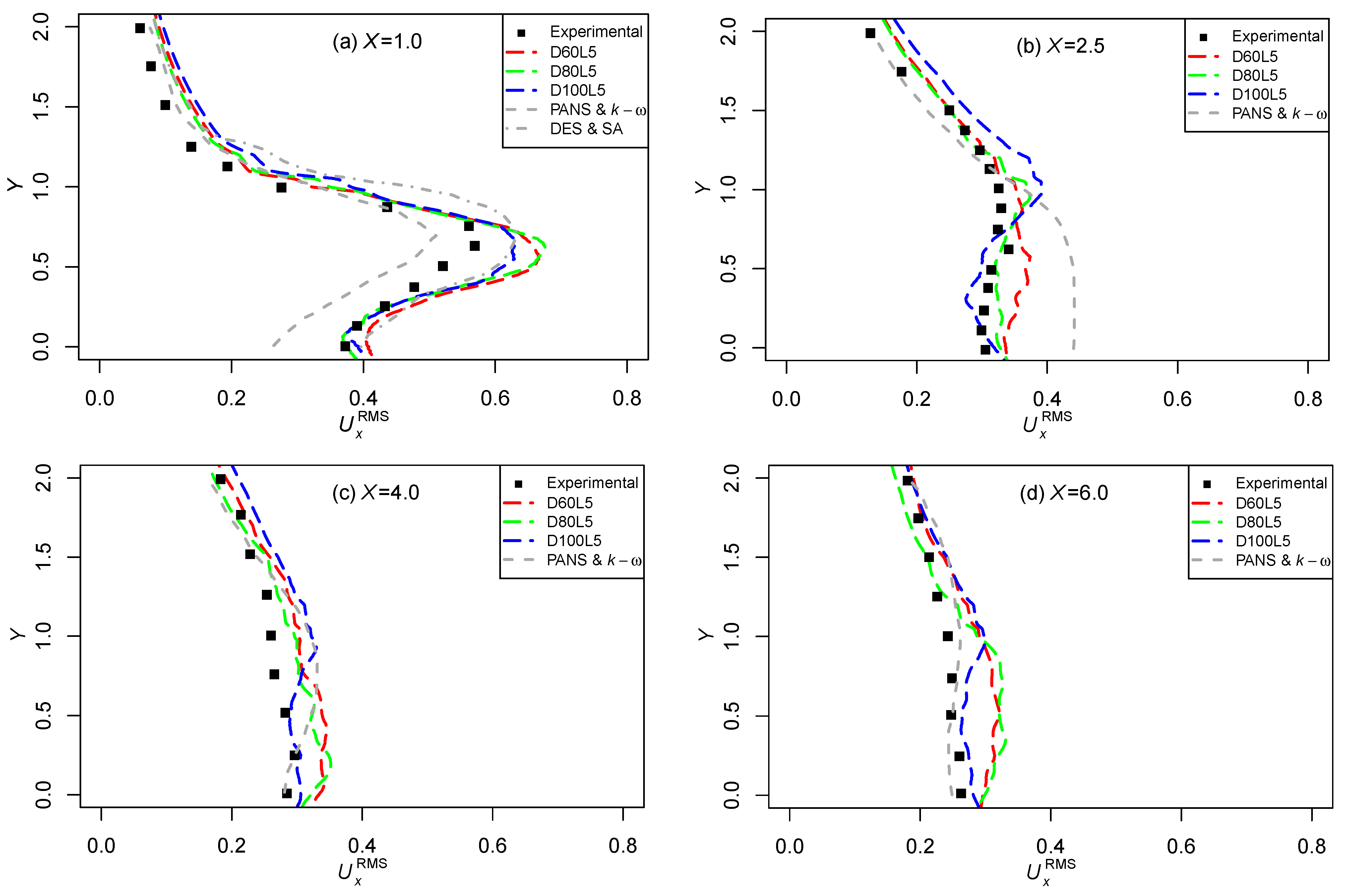
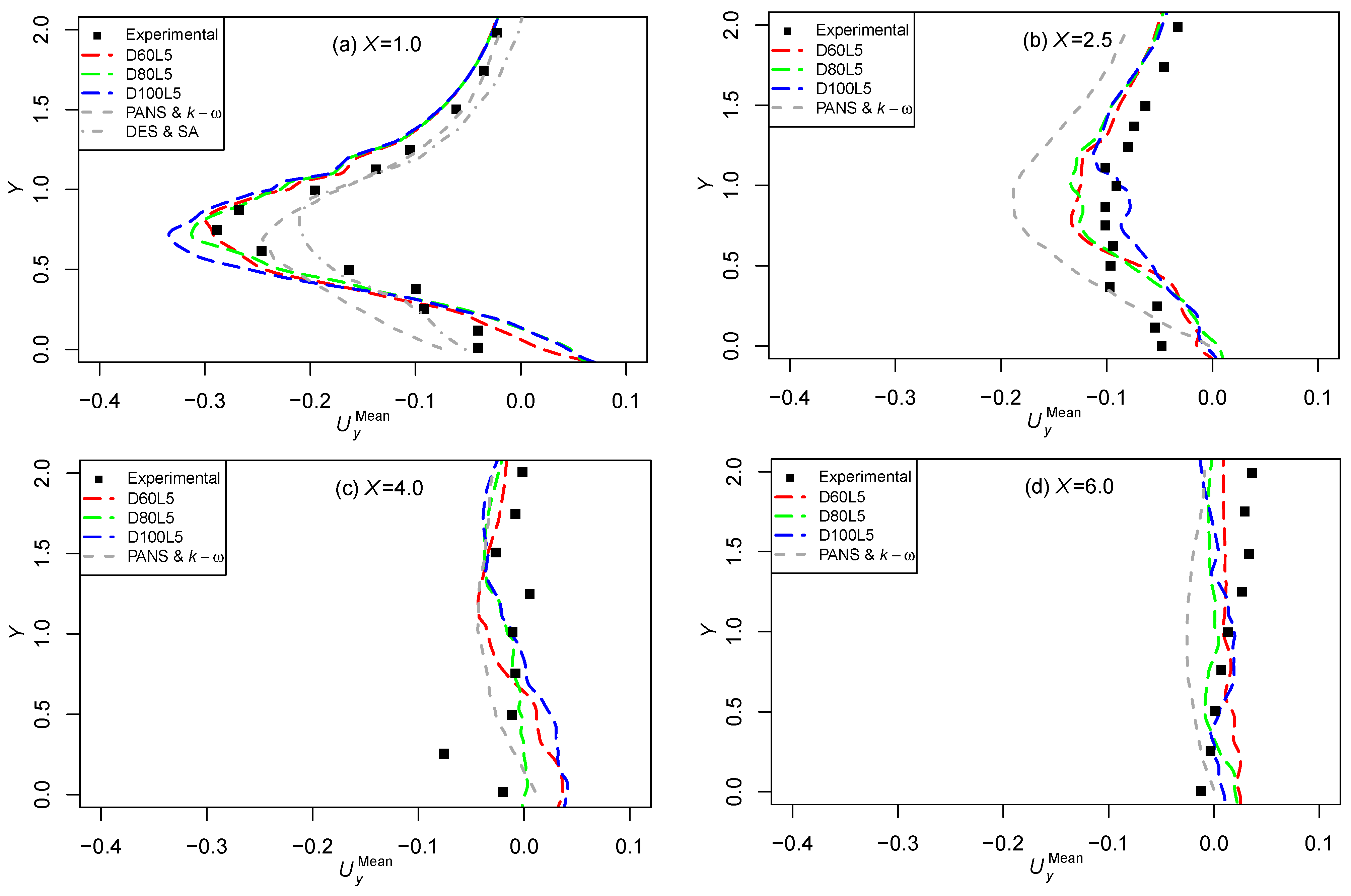
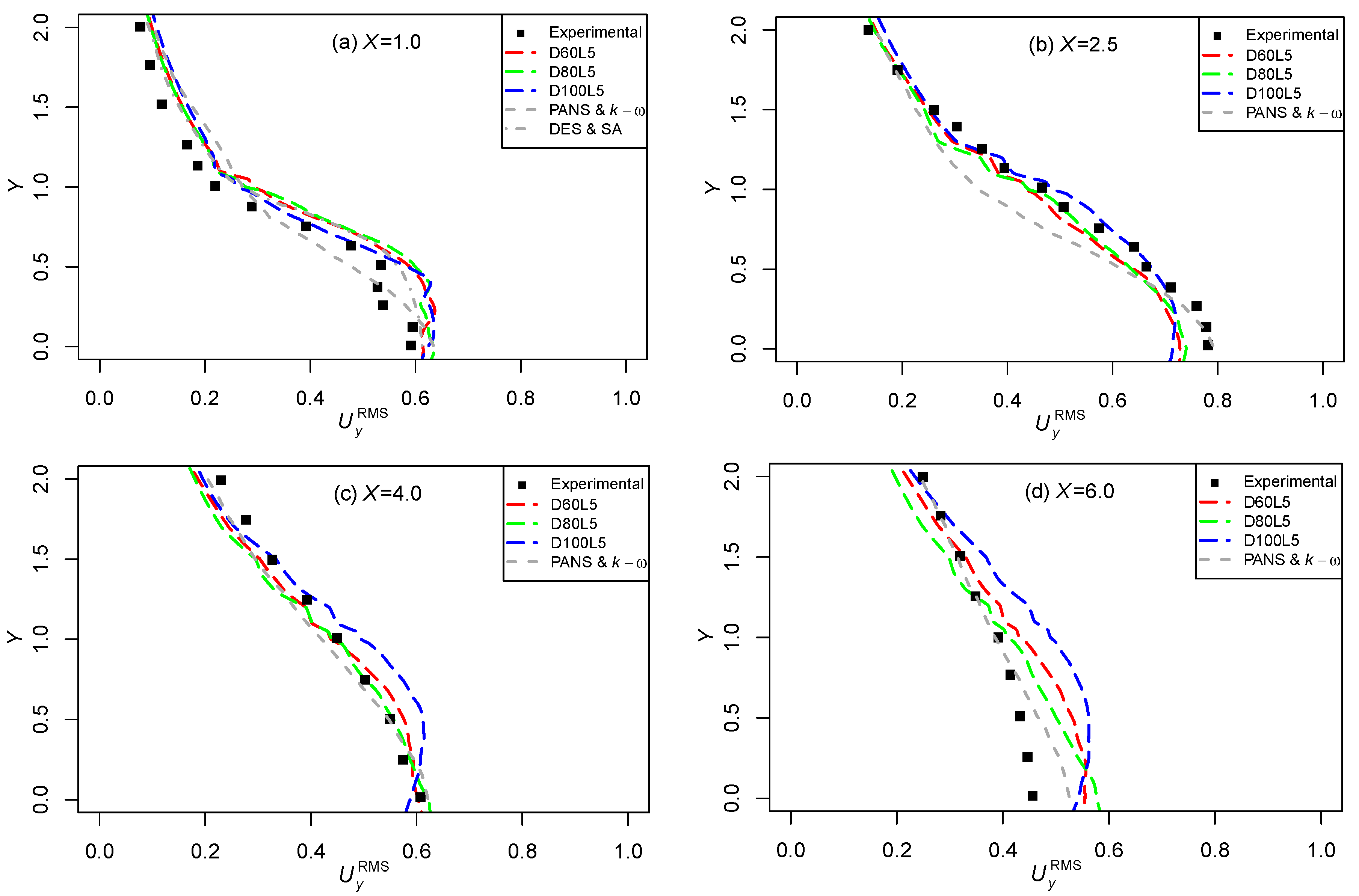
Figure 7, Figure 8, Figure 9 and Figure 10 show our results and their comparison with the data found in [8], as well as with the simulations by [19,24] (only reported for ). Our results are consistent between them and are in general agreement with the experimental data. For some cases in the near-middle wake, our simulations clearly reproduce the disturbed experimental flow better than the results reported in the literature (Figure 8a,b and Figure 9a,b), while being slightly worse in the near (Figure 7a), and far wake (Figure 7d, Figure 8d, and Figure 10d).
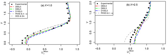
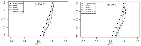
Figure 7.
Mean streamwise velocity along the transverse direction in different X’s lines of the wake. (a) . (b) . (c) . (d) .
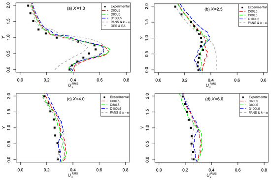
Figure 8.
RMS streamwise velocity along the transverse direction in different X’s lines of the wake. (a) . (b) . (c) . (d) .
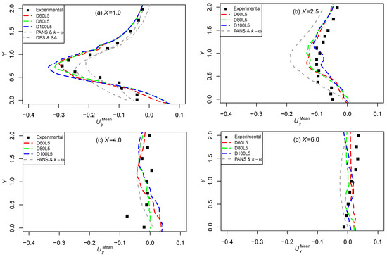
Figure 9.
RMS cross-stream velocity along the transverse direction in different X’s lines of the wake. (a) . (b) . (c) . (d) .
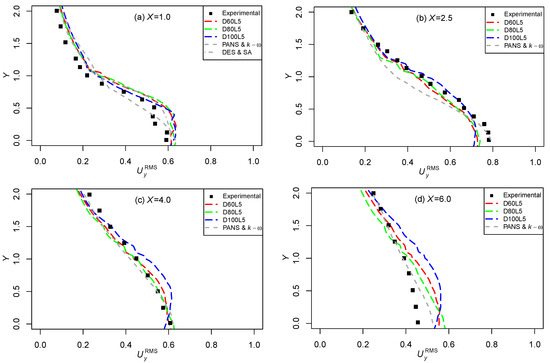
Figure 10.
RMS spanwise velocity along the transverse direction in different X’s lines of the wake. (a) . (b) . (c) . (d) .
Based on the results shown up to this point, we can say that the widest meshes (D80L5 and D100L5) converge and show consistency across all the variables and are more effective in capturing the flow patterns than the other narrower meshes (D20L5 and D40L5). The former also match the experimental results reported by [8], with more or less accuracy than previous simulation works, depending on the different zones of the analyzed flow. In contrast to heavy arrays, our meshes obtained acceptable results from 1.32 to 1.76 million cells (D60L5 and D80L5), which helped to minimize the computational cost.
3.2. Advances in Flow Characterization
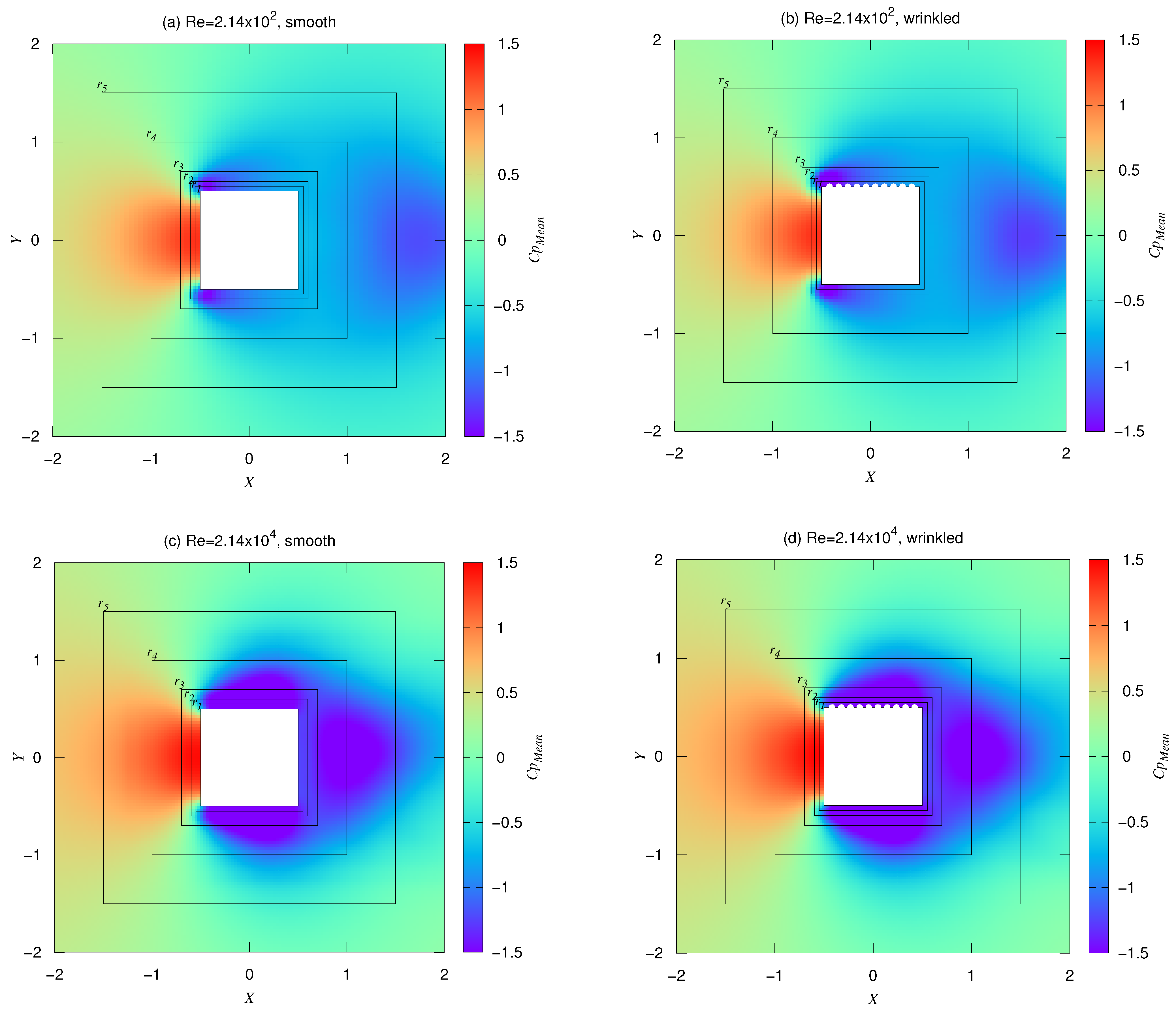
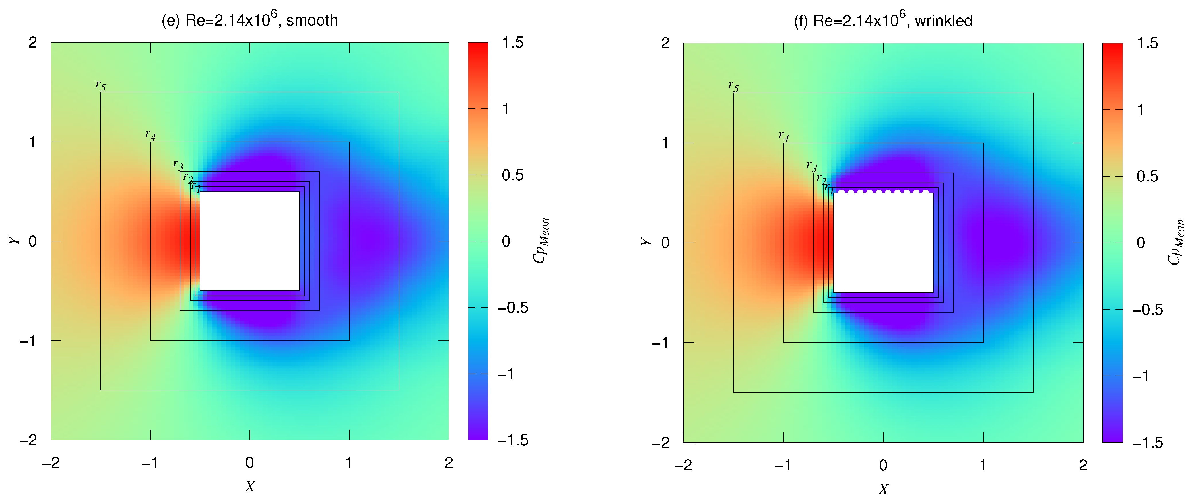
Techniques for improving visualization were compared in terms of how easily they conveyed essential and precise information of the flow around the cylinder. Figure 11 shows the most common way to report flow around an object—a time-averaged map of the pressure coefficients. Notwithstanding that this representation is useful to illustrate the general shape of high/low pressure zones of each picture, it is difficult to examine other characteristics, such as the delimitation and quantification of quick transitions, e.g., flow separation, near wake (), etc. Moreover, a comparison between maps shows that this form of representation is neither optimal for detecting flow disturbances induced by changes of Re, Figure 11c vs. Figure 11e, nor the asymmetries of a bluff body, Figure 11a,c,e vs. Figure 11b,d,f, respectively. In contrast, plotting the statistical variables along strategic lines, such as those represented in Figure 5, Figure 6, Figure 7, Figure 8, Figure 9 and Figure 10, represents a better alternative that tackles the issues of capturing the wake features highlighted above. Yet, this Cartesian representation does not fit well around the object, where the flow follows encircling patterns.

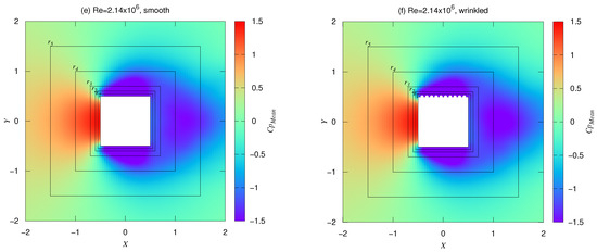
Figure 11.
Maps of the averaged coefficient pressure () around the cylinder for six study cases, noting the five dimensionless taxicab perimeters enclosing it: , , , , .
At this point, we discuss the use of polar charts by averaging the flow variables in concentric layers (shells) at different distances from the geometrical center of the object, which are highlighted by , , in the maps of Figure 11. A taxicab (or Manhattan) metric was selected to allow minimizing the difference in cells belonging to each angle interval for our object geometry. Nevertheless, another measure could be more suitable for different types of objects, e.g., the Euclidean distance for a circular cylinder.
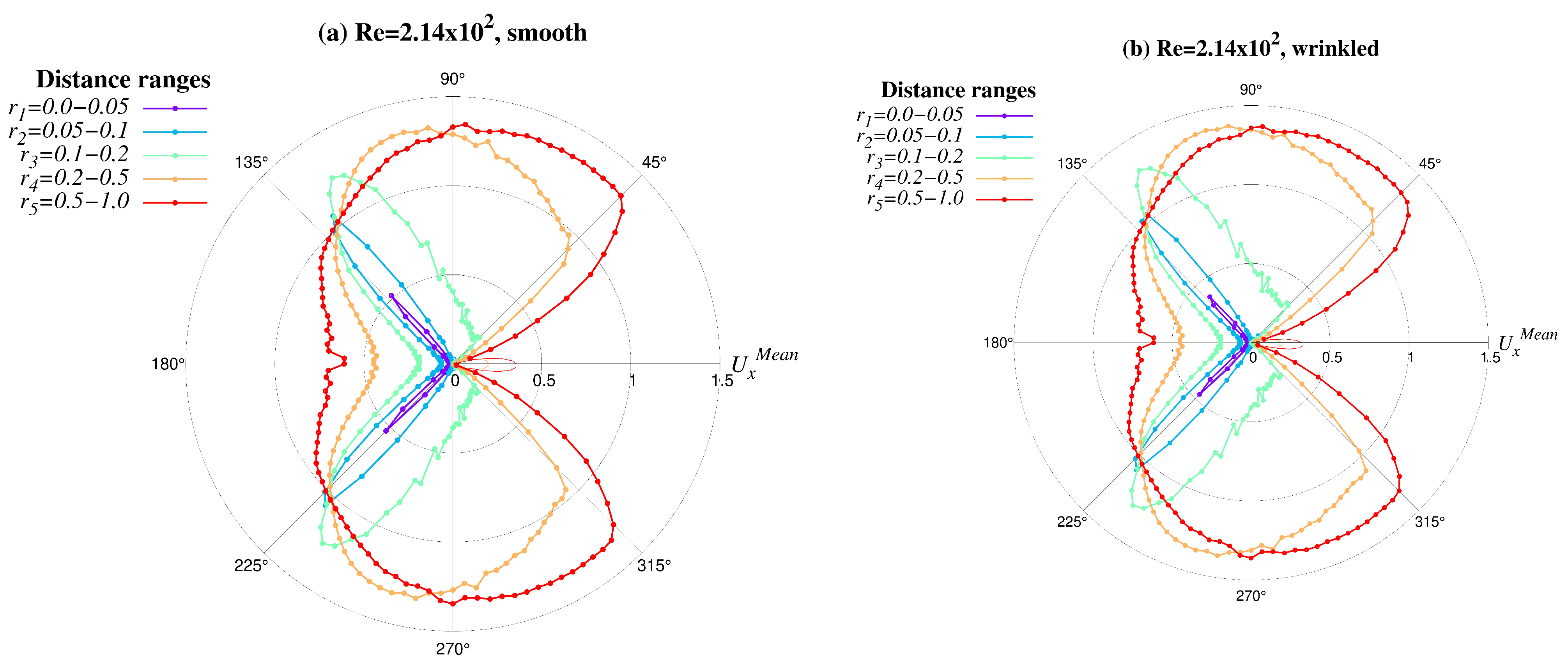
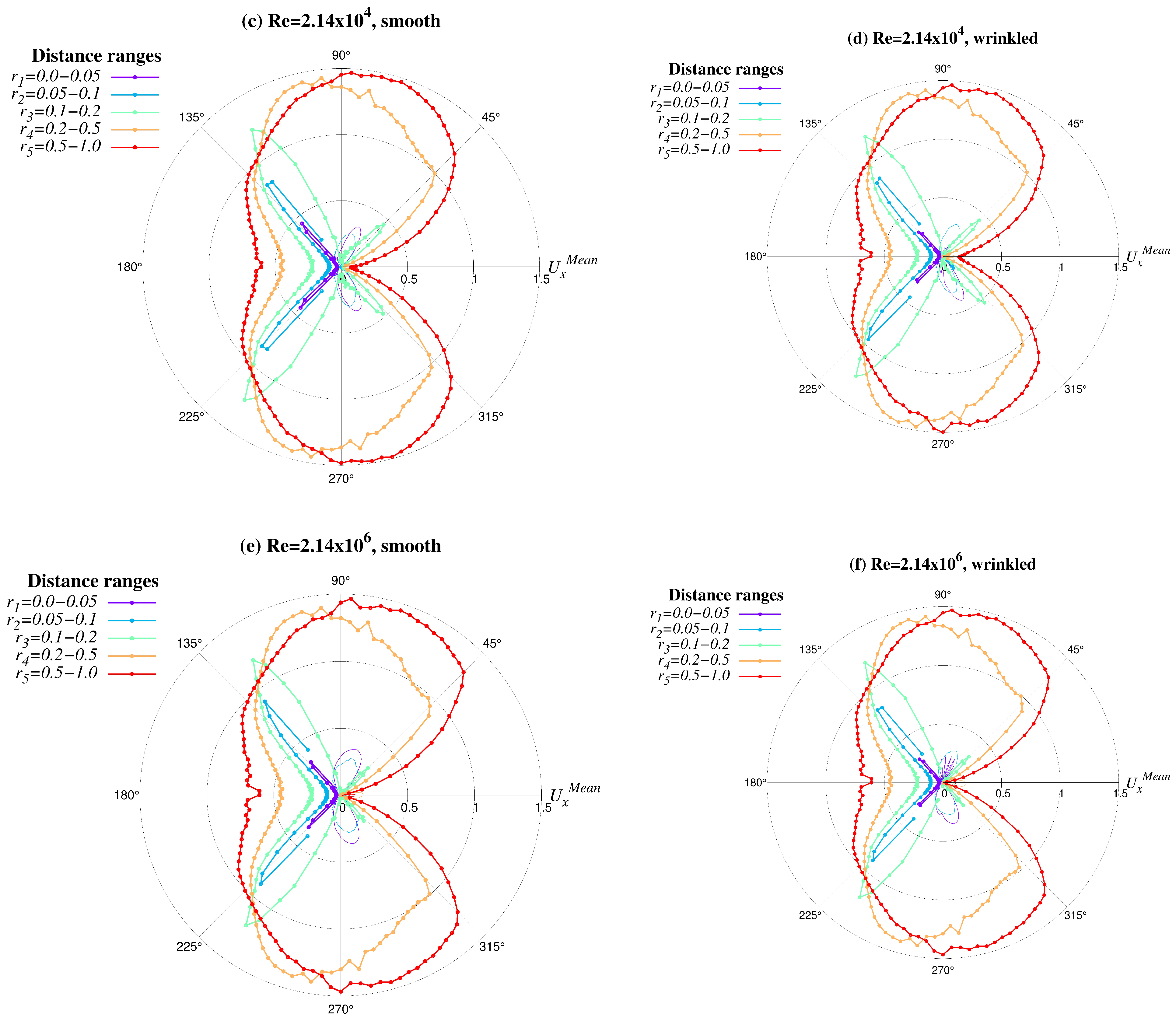
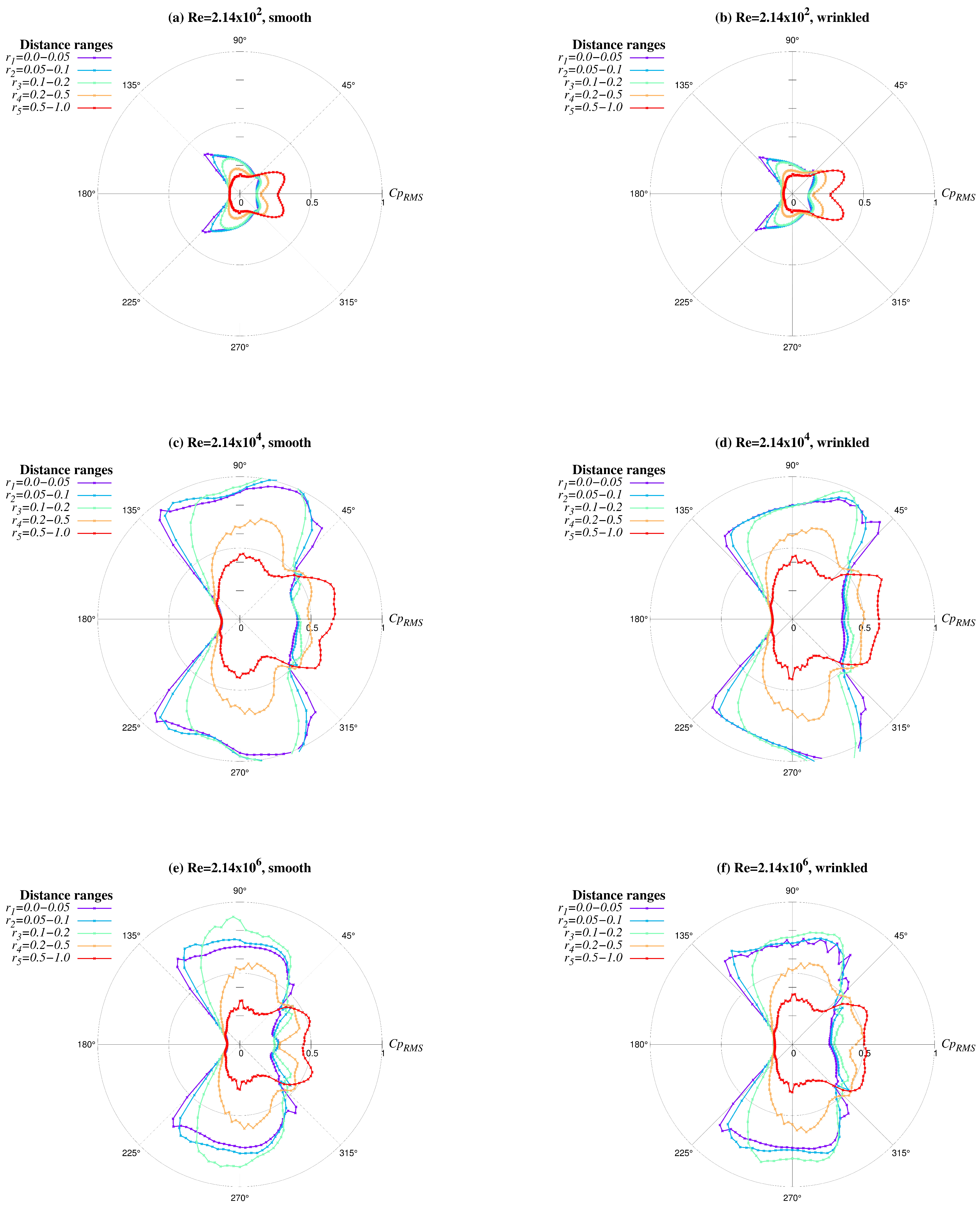
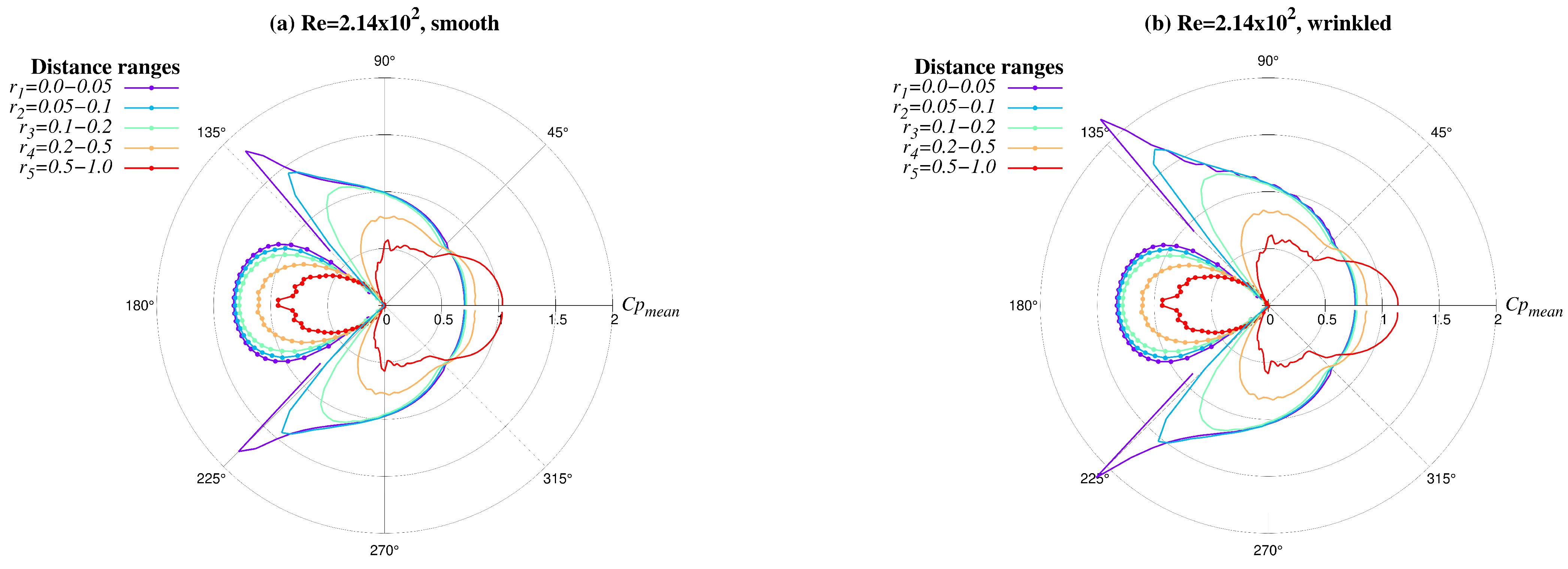
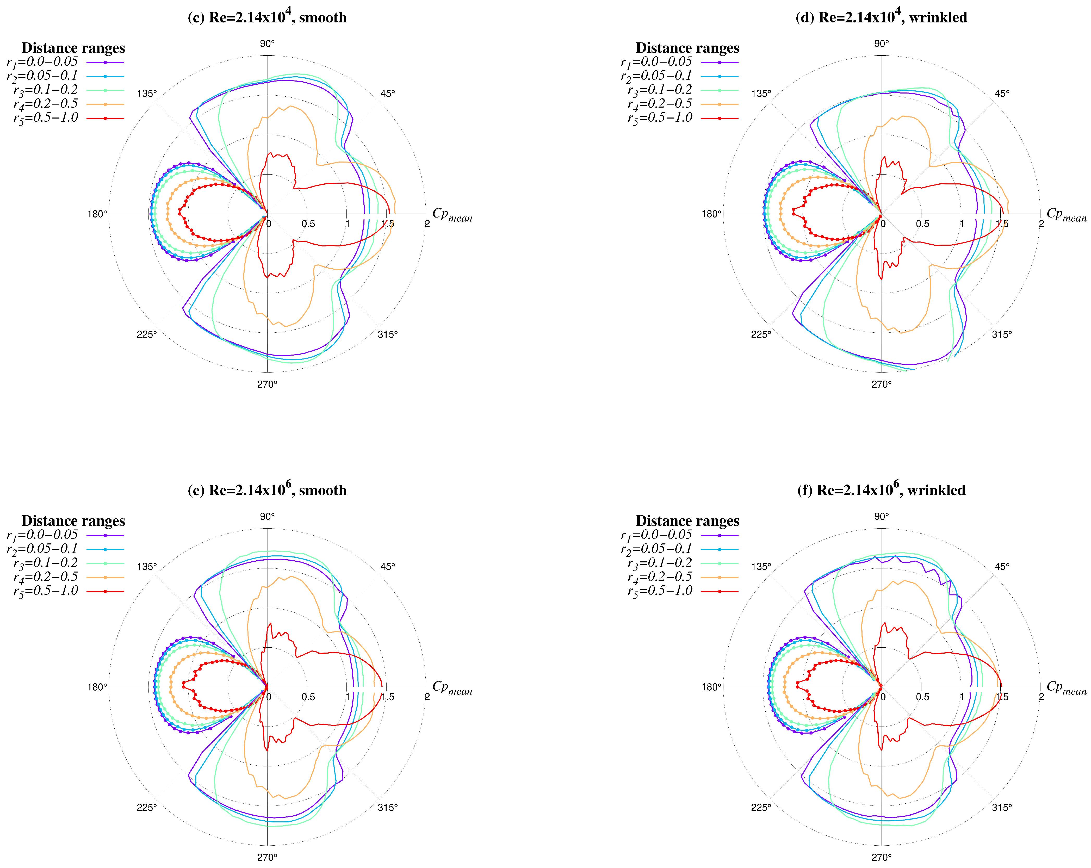
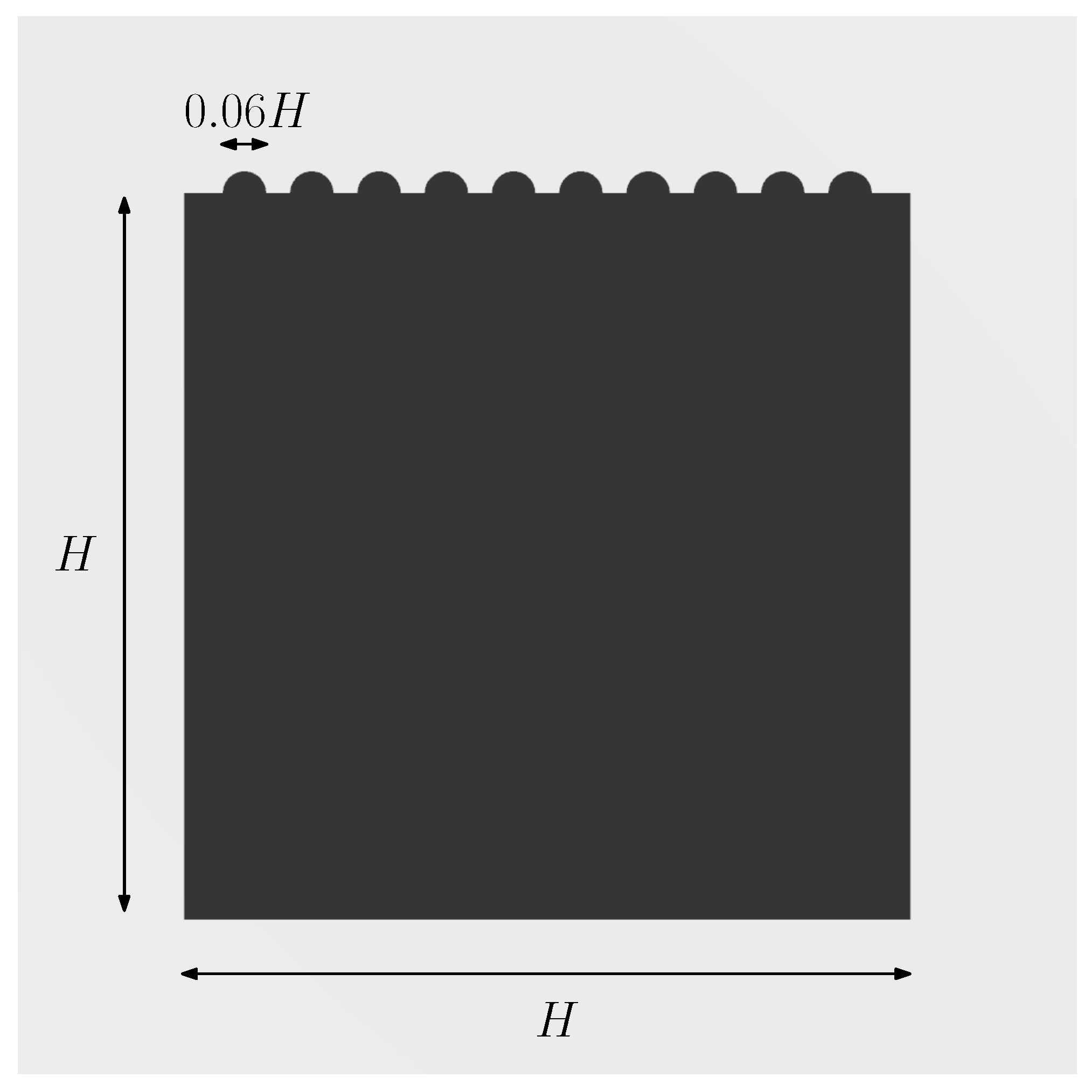
Figure 12 shows the resulting -patterns when using the new visualization approach, covering the range of cases Re = , with smooth and wrinkled surfaces, the latter achieved by adding deterministic-systematic roughness on the topside of the object. A total of 10 equispaced circular bumps with the same shape were placed (see Figure 13). Each bump is circumscribed to a cylinder of diameter equal to 6% of H that spans the main object in the spanwise direction.
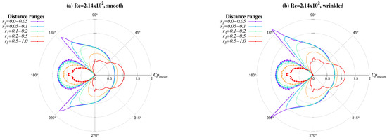
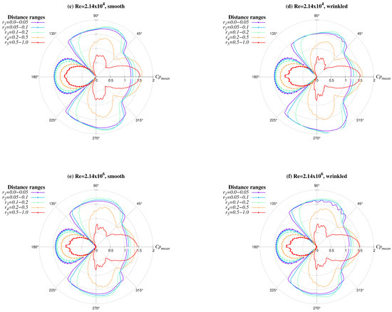
Figure 12.
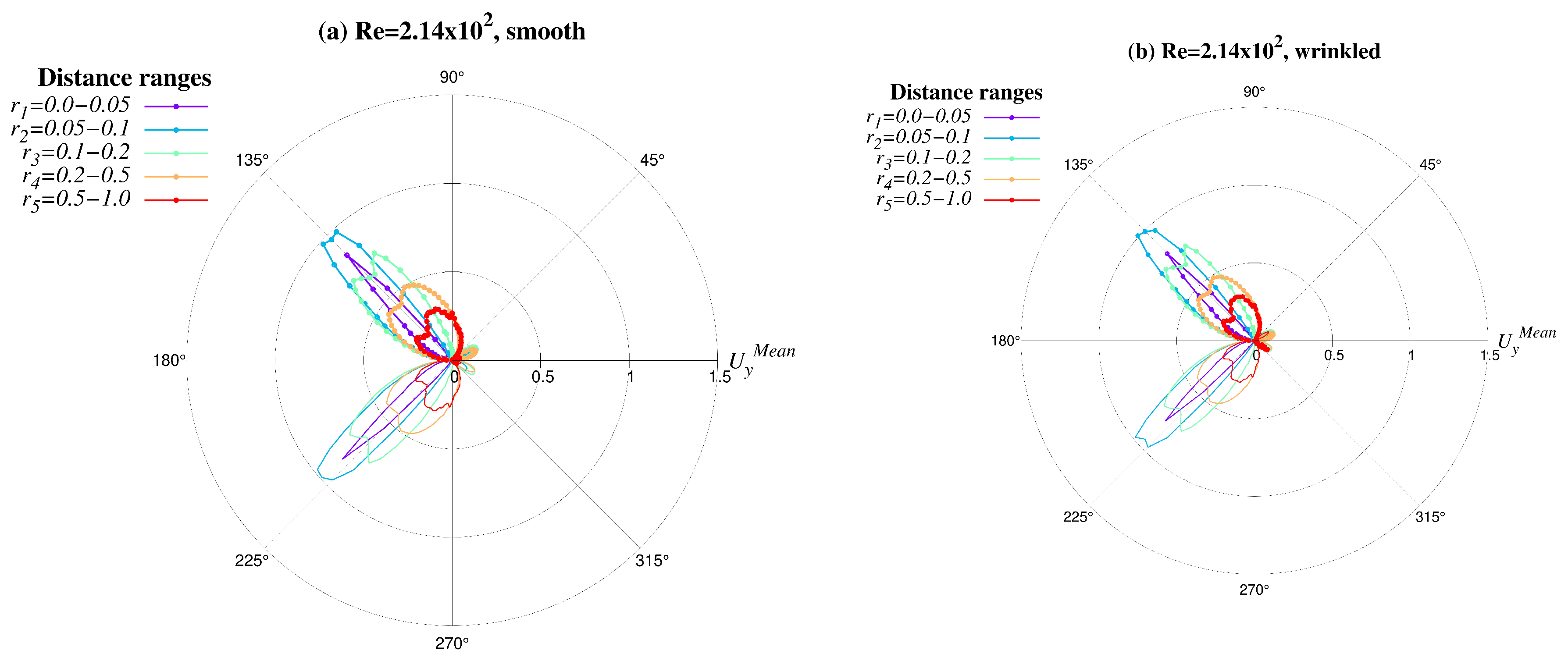
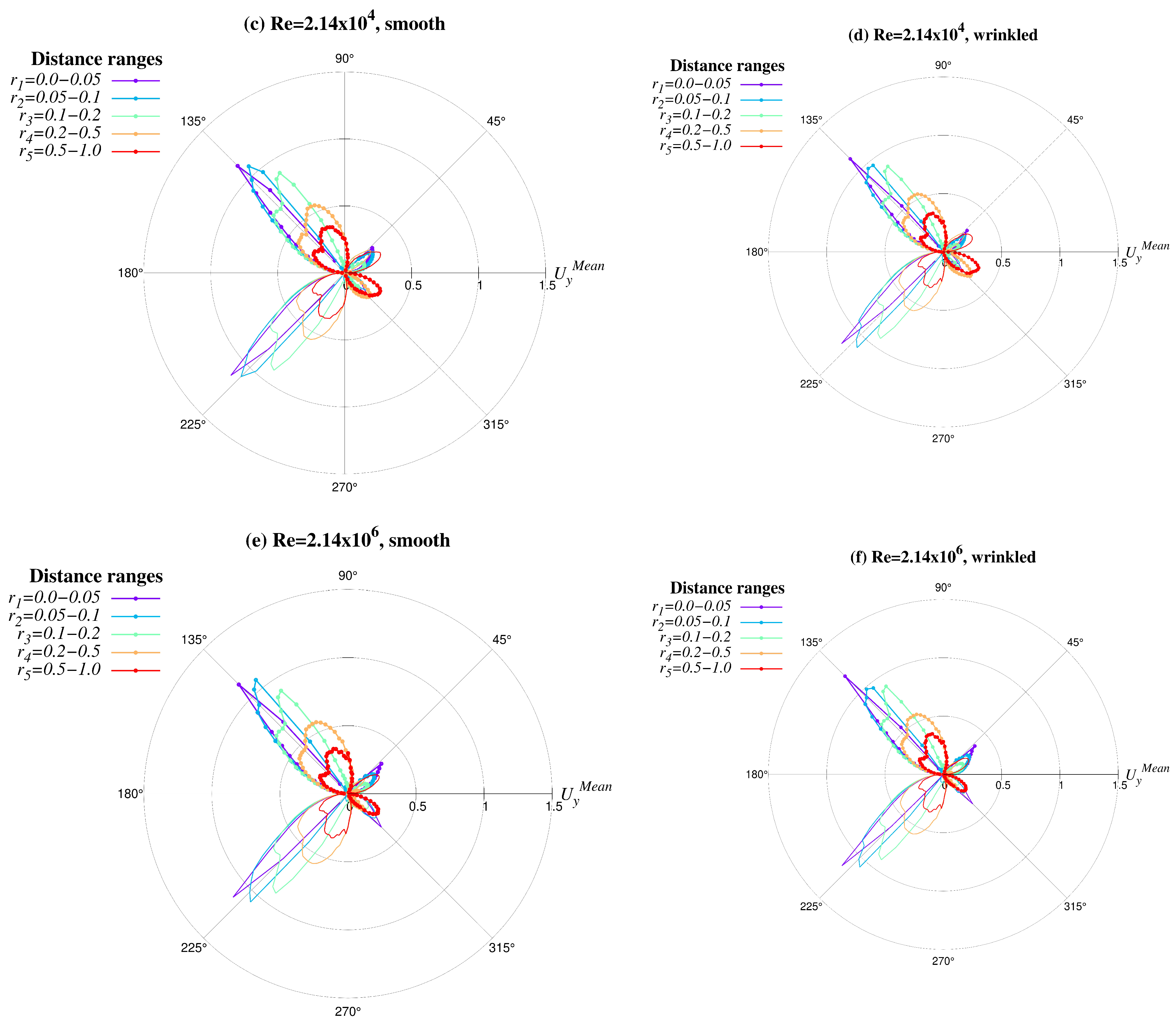
Flow patterns of for six study cases (a–f), averaged inside five dimensionless taxicab distance ranges, , . Negative values are plotted with smooth lines.
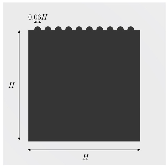
Figure 13.
Scheme of the non-smooth cylinder. The ten equally spaced bumps with diameter 0.06H cross the surface of the object in the spanwise direction.
Each bow in a chart represents the variable averaged at the corresponding shell, tagged by colors in the legend. The polar axis was discretized with a spacing of three degrees. The dot lines represent positive values and the smooth lines represent negative ones.
4. Discussion on the Visualization Technique
All charts of Figure 12 approximate the silhouette of a pigeon facing right but with particular characteristics. For example, at the lower Re, the unaltered flow near the top-rear side is reflected in the backward direction of the pigeon’s wings Figure 12a,b. This contrasts with the results derived from the medium and higher Re, which draw extended wings. The technique reveals additional features that distinguish the middle and higher Re, mainly at the top/bottom sides of the external (red) bow. It should be noted that the roughness of the cylinder is expressed mainly by local ripples on the internal (purple) bow Figure 12b,d,f.
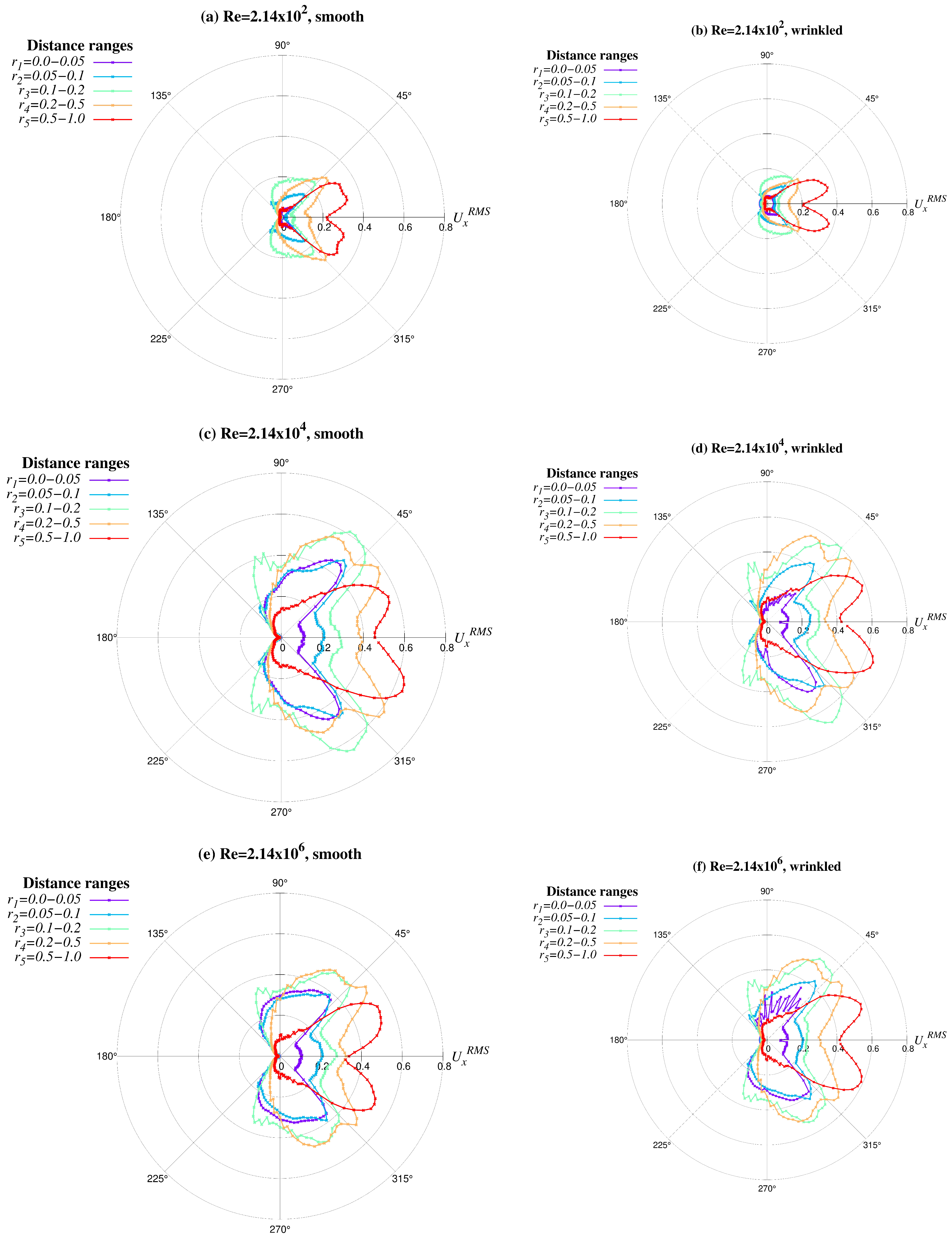
The complementary Figure A1, Figure A2, Figure A3, Figure A4 and Figure A5 in Appendix A were produced with the same visualization technique displayed in Figure 12, considering separate flow variables. As seen in these charts, the symmetry of flow disturbances also forms silhouettes of different flying insects and birds with the five bows, namely: —a butterfly spreading wings facing left; —a butterfly with wings in front; —a moth; —a beetle; and —a board type of bird/insect. Added to the highlights discussed above for the -patterns, it is worth noting that: (i) similar patterns could be observed across all study cases; (ii) each variable defines a different silhouette regardless of the Reynolds number or the slight increase in roughness; (iii) the magnitude of the RMS values is considerable higher for the middle and higher Re cases, which characterize the turbulence; (iv) a wrinkled cylinder causes sharpened shapes at the top and rear sides.
Now, through a finer analysis of the benchmark (Re = ), the flow patterns can be inferred from the different variables in Figure 12c, Figure A1c, Figure A2c, Figure A3c, Figure A4c and Figure A5c. Starting from in the clockwise direction, we observe near-zero values for all the velocity variables at the shortest taxicab distance—see the purple bows in Figure A1c, Figure A2c, Figure A3c and Figure A4c, which are related to the stagnation point lying around the highest positive pressure zones in Figure 12c, and the corresponding lowest variation in Figure A5c—all caused by the “first” impact of the fluid with the cylinder. Here, it is important to note that our visualizations effectively capture and enable quantifying the gradual increase and decrease in and for the same () direction but moving away from the object (bows ). The scrutiny also reveals a peak in the averaged velocities and a corresponding reversal of the averaged pressure at angles of about caused by the flow relief at the up-left corner of the square, differing in their transition to . Indeed, for , bows close to the object ( and ) return to near-zero values, while bows in the far encircling flow ( and ) reach the largest values, leading to the shape of a butterfly spreading wings; this represents the flow beyond the boundary layer that runs freely in the mainstream direction. In consequence, for , and settle to low values in that transition, leading to the butterfly with wings in front. In contrast to these velocity components and also in consequence of the above phenomenon, presents a sudden change in the high negative relative values in that transition (for incompressible flow, OpenFOAM supports expressing the pressure in comparison to the free-stream pressure defined, i.e., setting the zero-value to it), reaching its absolute maximum past .
Recirculation at the rear side (angles ) can be deduced from the contrast in the directions (line types) of the velocity components, also showing a peak in the values around and for and only at for , while both components return to zero-values at due to vorticity. In turn, the lowest pressure near the object is maintained up to around where a small rapid increment occurs. In contrast, the low pressure far from the object further decreases at to reach its lowest value at , shaping the pigeon’s head. We also note that, due to symmetry, the flow preserves the above characteristics at the bottom side of the object, including the corresponding change in direction for . Numerical asymmetry at the wake around the x- is easily observed for variables related to the -values, mainly for and .
In this way, while stressing that we are dealing with a benchmark problem, the above classification could facilitate the description (or dissemination) of the flow variables’ behavior, by stimulating metacognitive skills as a concise, practical, and easy-to-remember tool for technicians/students that need be familiarized with the problem or to verify the obtained solutions. Furthermore, the proposed technique opens up new avenues on flow characterization for scientists and engineers, for example, in defining inverse problems to connect flow disturbances to small-size modifications in object shape, or when looking to expand this pattern recognition methodology to non-symmetrical objects. Systematic studies considering different types of asymmetries are recommended for the exploration of the flow effects; this will be addressed in a forthcoming communication.
Finally, although a few of the above observations could be inferred from Figure 11, most could not be directly obtained and quantified from that picture, such as the precise location at which the changes occur, the flow asymmetries caused by the wrinkled surface, and the contrast between the positive and negative values that become lower since the color palette needs to cover a wider range of tones. In contrast, the combination of polar charts with the taxicab-metric-based shells enabled clear capture of most of these characteristics even through a laminar-turbulent transition. All this is supported by the fact that the insect/bird silhouettes are formed and maintained not only for but also stand for the other variables considered in the study.
5. Conclusions
We presented a flow visualization study on the simulation of flow around a smooth-square cylinder at three Reynolds numbers through the laminar-turbulent transition: Re = , and considering the respective cases with wrinkled cylinders. The investigation was firstly validated by a grid study considering five narrow computational arrays composed of structured and non-structured grids, varying the depth (z-axis). Guided by the thesis that narrowness affects the 3D-turbulence flow characteristics, we determined the optimal mesh that closely approximated the results published by other authors and which minimized the computational effort and file size.
Our visualization of the results consisted of projecting spatio-temporally average flow variables acting on shells on a polar domain. This enabled observation of patterns at different taxicab distances from the object that were not visible when using standard visualization techniques. The enhanced plots revealed significant details on the flow disturbances linked to the mean and RMS averaged values of the velocity and pressure, which otherwise translate on subtle gradients that are observable on the initial pressure maps. We, therefore, recommend the use of polar charts instead of traditional maps of variables for a better description of the flow around objects.
Notably, the novel flow patterns resembled what we called bird-shape and insect-like silhouettes that helped to enhance our understanding on the effect of lower (laminar flow) and higher (turbulent flow) Re on the pressure fields, even with the presence of roughness on the symmetric surface. The proposed technique also makes easier the recognition of patterns across the map and the identification of the controlling parameters. Similar visualization methodologies could be explored for other symmetric or quasi-symmetric objects.
Author Contributions
Conceptualization, M.A.A.-L. and F.H.-Z.; data curation, M.A.A.-L. and F.H.-Z.; formal analysis, M.A.A.-L., F.H.-Z. and P.M.-V.; funding acquisition, P.M.-V.; investigation, M.A.A.-L. and F.H.-Z.; methodology, M.A.A.-L., F.H.-Z. and P.M.-V.; project administration, F.H.-Z.; resources, M.A.A.-L.; software, M.A.A.-L.; supervision, F.H.-Z. and P.M.-V.; validation, F.H.-Z. and P.M.-V.; visualization, M.A.A.-L. and F.H.-Z.; writing—original draft, M.A.A.-L.; writing—review and editing, F.H.-Z. and P.M.-V. All authors have read and agreed to the published version of the manuscript.
Funding
This research was funded by Consejo Nacional de Humanidades Ciencias y Tecnologías (CONAHCyT) grant number 839412. The APC was supported by The University of Birmingham. The third author gratefully acknowledges the support of The Royal Society towards the mobility grant IES\R1\221087.
Institutional Review Board Statement
Not applicable.
Informed Consent Statement
Not applicable.
Data Availability Statement
The data presented in this study are available on request from the corresponding author. The data are not publicly available due to their large size.
Acknowledgments
The authors thankfully acknowledge the computer resources, technical expertise and support provided by the Laboratorio Nacional de Supercómputo del Sureste de México, CONAHCyT member of the Network of National Laboratories. The second author thanks FCFM-UNACH and the support from CONAHCyT through the program “Investigadoras e investigadores por México”, Cátedra 873.
Conflicts of Interest
The authors declare no conflicts of interest.
Appendix A. Flow Encircling Patterns
Appendix A.1. —Butterfly (Spreading Wings)
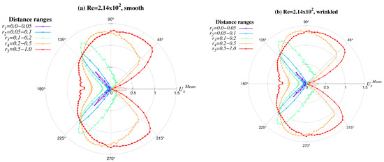
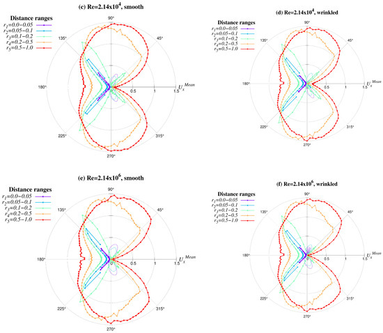
Figure A1.
Flow patterns of for six study cases (a–f), averaged inside five dimensionless taxicab distance ranges, , . Negative values are plotted with smooth lines.
Figure A1.
Flow patterns of for six study cases (a–f), averaged inside five dimensionless taxicab distance ranges, , . Negative values are plotted with smooth lines.
Appendix A.2. —Butterfly (Wings in Front)
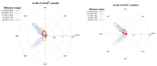
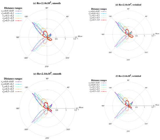
Figure A2.
Flow patterns of for six study cases (a–f), averaged inside five dimensionless taxicab distance ranges, , . Negative values are plotted with smooth lines.
Figure A2.
Flow patterns of for six study cases (a–f), averaged inside five dimensionless taxicab distance ranges, , . Negative values are plotted with smooth lines.
Appendix A.3. —Moth
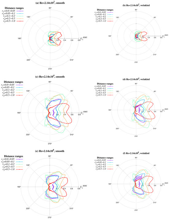
Figure A3.
Flow patterns of for six study cases (a–f), averaged inside five dimensionless taxicab distance ranges, , .
Figure A3.
Flow patterns of for six study cases (a–f), averaged inside five dimensionless taxicab distance ranges, , .
Appendix A.4. —Beetle
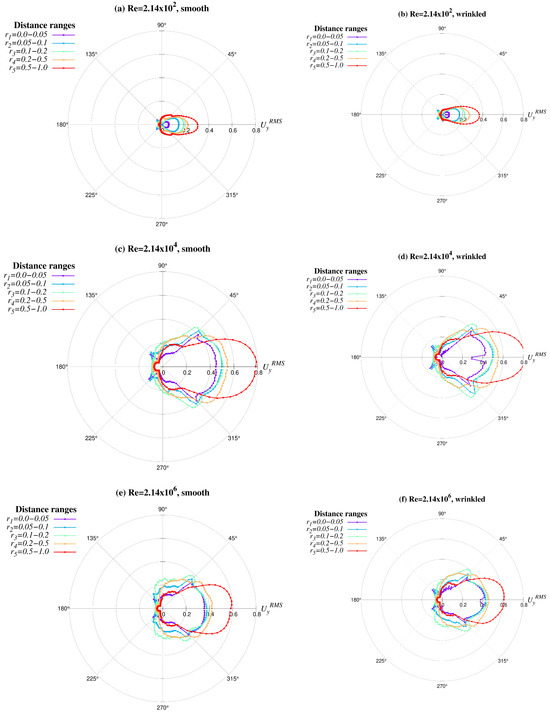
Figure A4.
Flow patterns of for six study cases (a–f), averaged inside five dimensionless taxicab distance ranges, , .
Figure A4.
Flow patterns of for six study cases (a–f), averaged inside five dimensionless taxicab distance ranges, , .
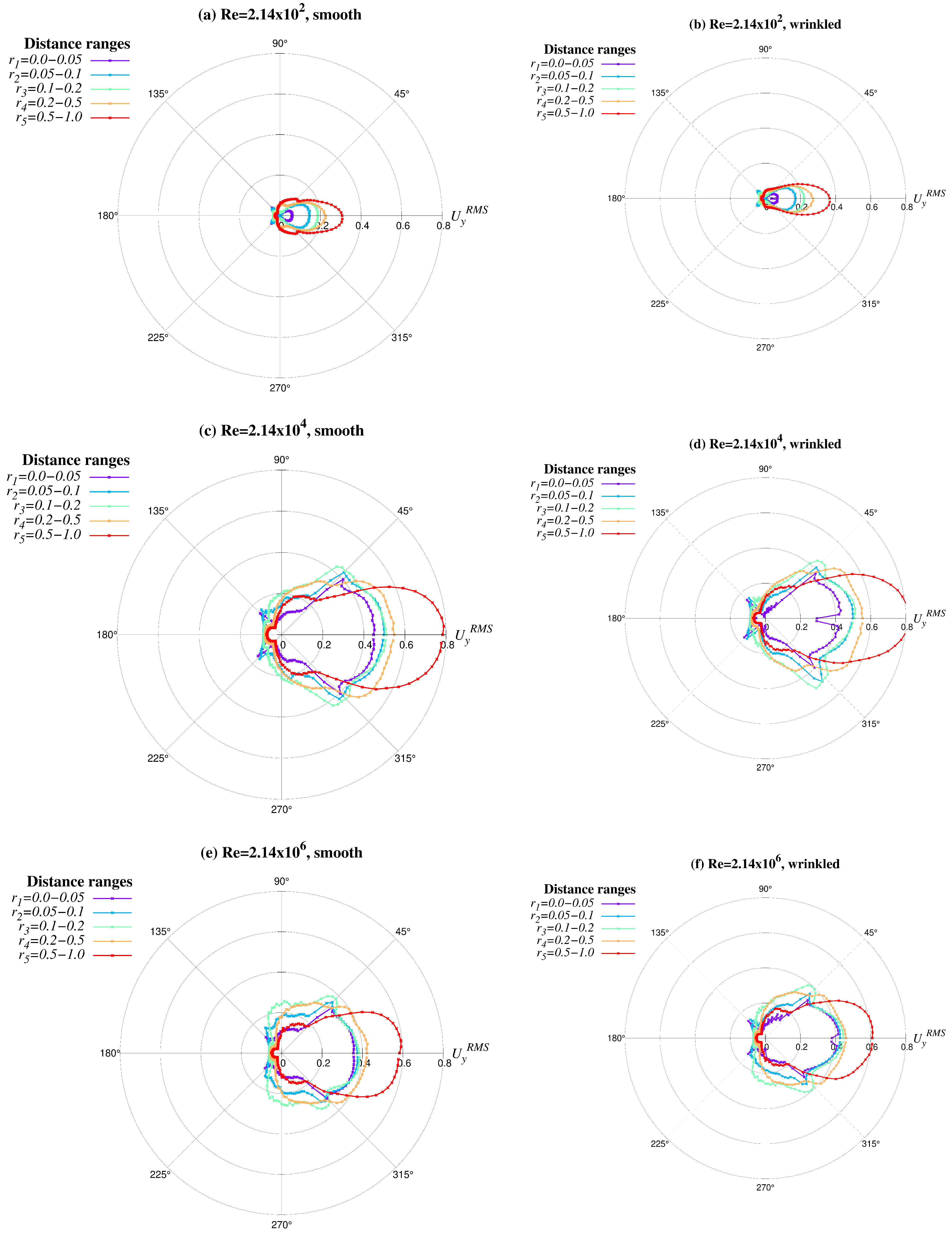
Appendix A.5. —Board Bird/Insect
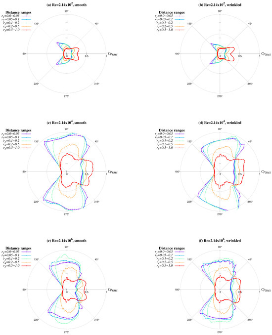
Figure A5.
Flow patterns of for six study cases (a–f), averaged inside five dimensionless taxicab distance ranges, , .
Figure A5.
Flow patterns of for six study cases (a–f), averaged inside five dimensionless taxicab distance ranges, , .
References
- Jin, Y.; Cheng, Z.; Han, X.; Mao, J.; Jin, F. VLES of drag reduction for high Reynolds number flow past a square cylinder based on OpenFOAM. Ocean. Eng. 2019, 190, 106450. [Google Scholar] [CrossRef]
- Shi, X.; Dong, J.; Yan, G.; Zhu, C. Flow around a Rectangular Cylinder Placed in a Channel with a High Blockage Ratio under a Subcritical Reynolds Number. Water 2021, 13, 3388. [Google Scholar] [CrossRef]
- Mazellier, N.; Feuvrier, A.; Kourta, A. Biomimetic bluff body drag reduction by self-adaptive porous flaps. Comptes Rendus MéCanique 2012, 340, 81–94. [Google Scholar] [CrossRef]
- Malekzadeh, S.; Mirzaee, I.; Pourmahmoud, N.; Shirvani, H. The passive control of three-dimensional flow over a square cylinder by a vertical plate at a moderate Reynolds number. Fluid Dyn. Res. 2017, 49, 025515. [Google Scholar] [CrossRef]
- Damissie, H.Y.; Babu, N.R. Aerodynamic Drag Reduction on Locally Built Bus Body using Computational Fluid Dynamics (CFD): A Case Study at Bishoftu Automotive Industry. Int. J. Eng. Res. Technol. 2017, 6, 276–283. [Google Scholar]
- Modi, V.; Hill, S.; Yokomizo, T. Drag reduction of trucks through boundary-layer control. J. Wind. Eng. Ind. Aerodyn. 1995, 54–55, 583–594. [Google Scholar] [CrossRef]
- Altaf, A.; Omar, A.A.; Asrar, W. Passive drag reduction of square back road vehicles. J. Wind. Eng. Ind. Aerodyn. 2014, 134, 30–43. [Google Scholar] [CrossRef]
- Lyn, D.A.; Einav, S.; Rodi, W.; Park, J.H. A laser-Doppler velocimetry study of ensemble-averaged characteristics of the turbulent near wake of a square cylinder. J. Fluid Mech. 1995, 304, 285–319. [Google Scholar] [CrossRef]
- Norberg, C. Flow around rectangular cylinders: Pressure forces and wake frequencies. J. Wind. Eng. Ind. Aerodyn. 1993, 49, 187–196. [Google Scholar] [CrossRef]
- Luo, S.; Yazdani, M.; Chew, Y.; Lee, T. Effects of incidence and afterbody shape on flow past bluff cylinders. J. Wind. Eng. Ind. Aerodyn. 1994, 53, 375–399. [Google Scholar] [CrossRef]
- Minguez, M.; Brun, C.; Pasquetti, R.; Serre, E. Experimental and high-order LES analysis of the flow in near-wall region of a square cylinder. Int. J. Heat Fluid Flow 2011, 32, 558–566. [Google Scholar] [CrossRef]
- Durão, D.F.G.; Heitor, M.V.; Pereira, J.C.F. Measurements of turbulent and periodic flows around a square cross-section cylinder. Exp. Fluids 1988, 6, 298–304. [Google Scholar] [CrossRef]
- van Oudheusden, B.; Scarano, F.; van Hinsberg, N.; Roosenboom, E. Quantitative visualization of the flow around a square-section cylinder at incidence. J. Wind. Eng. Ind. Aerodyn. 2008, 96, 913–922. [Google Scholar] [CrossRef]
- Cao, Y.; Tamura, T. Aerodynamic characteristics of a rounded-corner square cylinder in shear flow at subcritical and supercritical Reynolds numbers. J. Fluids Struct. 2018, 82, 473–491. [Google Scholar] [CrossRef]
- Liu, J.; Hui, Y.; Yang, Q.; Tamura, Y. Flow field investigation for aerodynamic effects of surface mounted ribs on square-sectioned high-rise buildings. J. Wind. Eng. Ind. Aerodyn. 2021, 211, 104551. [Google Scholar] [CrossRef]
- Liu, J.; Hui, Y.; Yang, Q.; Zhang, R. LES evaluation of the aerodynamic characteristics of high-rise building with horizontal ribs under atmospheric boundary layer flow. J. Build. Eng. 2023, 71, 106487. [Google Scholar] [CrossRef]
- Chollet, J.P.; Voke, P.R.; Kleiser, L. Direct and Large-Eddy Simulation II; Springer: Berlin/Heidelberg, Germany, 1997. [Google Scholar]
- Ke, J. RANS and hybrid LES/RANS simulations of flow over a square cylinder. Adv. Aerodyn. 2019, 1, 10. [Google Scholar] [CrossRef]
- Barone, M.F.; Roy, C.J. Evaluation of Detached Eddy Simulation for Turbulent Wake Applications. AIAA J. 2006, 44, 3062–3071. [Google Scholar] [CrossRef]
- Srinivas, Y.; Biswas, G.; Parihar, A.S.; Ranjan, R. Large-Eddy Simulation of High Reynolds Number Turbulent Flow Past a Square Cylinder. J. Eng. Mech. 2006, 132, 327–335. [Google Scholar] [CrossRef]
- Jiao, J.; Zhang, Y. Multiscale subgrid models of large eddy simulation for turbulent flows. Int. J. Numer. Methods Heat Fluid Flow 2016, 26, 1380–1390. [Google Scholar] [CrossRef]
- Sohankar, A.; Davidson, L.; Norberg, C. Large Eddy Simulation of Flow Past a Square Cylinder: Comparison of Different Subgrid Scale Models. J. Fluids Eng. Trans. ASME 2000, 122, 39–47. [Google Scholar] [CrossRef]
- Anton, A. Numerical Investigation of Unsteady Flows Using OpenFOAM. Hidraul. Mag. Hydraul. Pneum. Tribol. Ecol. Sens. Mechatronics 2016, 1, 7–12. [Google Scholar]
- Chakraborty, A.; Warrior, H. Study of turbulent flow past a square cylinder using partially-averaged Navier–Stokes method in OpenFOAM. Proc. Inst. Mech. Eng. Part C J. Mech. Eng. Sci. 2020, 234, 2821–2832. [Google Scholar] [CrossRef]
- Saroha, S.; Chakraborty, K.; Sinha, S.S.; Lakshmipathy, S. An OpenFOAM-Based Evaluation of PANS Methodology in Conjunction with Non-Linear Eddy Viscosity: Flow Past a Heated Cylinder. J. Appl. Fluid Mech. 2020, 13, 1453–1469. [Google Scholar] [CrossRef]
- Wenneker, I. Computation of Flows Using Unstructured Staggered Grids. Ph.D Thesis, Delft University of Technology, Faculty of Electrical Engineering, Mathematics and Computer Science, Delft, The Netherlands, 2002. [Google Scholar]
- Lodh, B.; Das, A.; Singh, N. Investigation of Turbulence for Wind Flow over a Surface Mounted Cube using Wall Y+ Approach. Indian J. Sci. Technol. 2017, 10, 1–11. [Google Scholar] [CrossRef]
- OpenFOAM. OpenCFD Release OpenFOAM v2012. 2020. Available online: https://www.openfoam.com/news/main-news/openfoam-v20-12 (accessed on 1 January 2021).
- Spalart, P.; Allmaras, S. A one-equation turbulence model for aerodynamic flows. In Proceedings of the 30th Aerospace Sciences Meeting and Exhibit, Reno, NV, USA, 6–9 January 1992; American Institute of Aeronautics and Astronautics: Reston, VA, USA, 1992; pp. 1–22. [Google Scholar] [CrossRef]
- Spalart, P.R.; Deck, S.; Shur, M.L.; Squires, K.D.; Strelets, M.K.; Travin, A. A New Version of Detached-eddy Simulation, Resistant to Ambiguous Grid Densities. Theor. Comput. Fluid Dyn. 2006, 20, 181–195. [Google Scholar] [CrossRef]
- OpenFOAM v2012. Spalart-Allmaras Delayed Detached Eddy Simulation (DDES). 2020. Available online: https://www.openfoam.com/documentation/guides/v2012/doc/guide-turbulence-des-spalart-allmaras-ddes.html (accessed on 1 May 2021).
- OpenFOAM v2012. Spalart-Allmaras Detached Eddy Simulation (DES). 2020. Available online: https://www.openfoam.com/documentation/guides/v2012/doc/guide-turbulence-des-spalart-allmaras-des.html (accessed on 1 May 2021).
- Muhammad, N.; Lashin, M.M.A.; Alkhatib, S. Simulation of turbulence flow in OpenFOAM using the large eddy simulation model. Proc. Inst. Mech. Eng. Part E J. Process Mech. Eng. 2022, 236, 2252–2265. [Google Scholar] [CrossRef]
- Muhammad, N.; Alharbi, K.A.M. OpenFOAM for computational hydrodynamics using finite volume method. Int. J. Mod. Phys. B 2023, 37, 2350026. [Google Scholar] [CrossRef]
- OpenFOAM v2112. pisoFOAM Solver. 2018. Available online: https://www.openfoam.com/documentation/guides/latest/doc/guide-applications-solvers-incompressible-pisoFoam.html (accessed on 1 May 2021).
- Issa, R. Solution of the implicitly discretised fluid flow equations by operator-splitting. J. Comput. Phys. 1986, 62, 40–65. [Google Scholar] [CrossRef]
- Issa, R.; Gosman, A.; Watkins, A. The computation of compressible and incompressible recirculating flows by a non-iterative implicit scheme. J. Comput. Phys. 1986, 62, 66–82. [Google Scholar] [CrossRef]
- OpenFOAM. Repository of Tutorials. 2016. Available online: https://develop.openfoam.com/Development/openfoam/-/tree/master/tutorials (accessed on 1 March 2021).
- FreeCAD. FreeCAD. Your Own 3D Parametric Modeler, Version 2018. Available online: https://www.freecad.org/ (accessed on 1 January 2022).
- NASA Langely Research Center. Turbulence Modeling Resource. The Spalart-Allmaras Turbulence Model. 2020. Available online: https://turbmodels.larc.nasa.gov/spalart.html (accessed on 1 May 2021).
Disclaimer/Publisher’s Note: The statements, opinions and data contained in all publications are solely those of the individual author(s) and contributor(s) and not of MDPI and/or the editor(s). MDPI and/or the editor(s) disclaim responsibility for any injury to people or property resulting from any ideas, methods, instructions or products referred to in the content. |
© 2023 by the authors. Licensee MDPI, Basel, Switzerland. This article is an open access article distributed under the terms and conditions of the Creative Commons Attribution (CC BY) license (https://creativecommons.org/licenses/by/4.0/).