Abstract
Quantum Parameter Estimation (QPE) is commonly led using quantum probe states for the characterization of quantum systems. For these purposes, Quantum Fisher Information (QFI) plays a crucial role by imposing a lower bound for the parametric estimation of quantum channels. Several schemes for obtaining QFI lower bounds have been proposed, particularly for Pauli channels regarding qubits. Those schemes commonly employ either the individual channel, multiple copies of it, or arrangements including communication architectures. The present work aims to propose an architecture involving path superposition and causal indefinite order in superposition. Thus, by controlling the symmetry balance of this superposition, it reaches notable improvements in quantum parameter estimation. The proposed architecture has been tested to find the best possible QPE bounds for a representative and emblematic set of Pauli channels. Further, for the most reluctant channels, it was revisited testing the architecture again under a primary path superposition (using double teleportation) and also using entangled probe states to recombine their outputs with the original undisturbed state. Notable outcomes practically near zero were found for the QPE bounds, stating a hierarchy between the approaches, but anyway reaching a perfect theoretical QPE, particularly for the last path superposition including the proposed architecture.
1. Introduction
The structure of quantum systems is determined by parameters affecting their interactions with external systems. The knowledge of these parameters can be obtained from intermediate measurements that capture features inherited from these interactions. Parameters could characterize several applied systems as cute sensors [1], featured physical interactions or processes [2], as well as communication channels [3]. For the classical transmission of information, the Fisher information [4] measures the amount of information provided by a random variable associated with an unknown parameter of a statistical distribution, while the quantum analog, the Quantum Fisher Information (QFI) [5], is an extension of this concept used to estimate parameters associated with quantum processes through observable measurements.
The Cramér–Rao Bound (CRB) [6,7] involves Fisher information, whether classical or quantum, to set a limit for the variance associated with the Quantum Parameter Estimation (QPE) process. The QFI thus states a bound for the knowledge of channel parameters. Quantum channels can be characterized using parameters that modify the initial probe state into an outcome coming from the target system. Therefore, QFI is useful in characterizing quantum channels.
Among such channels, the Pauli channels are commonly used in quantum information and communication involving qubits. These channels have been extensively studied due to their affordability and can be characterized by three independent parameters. These channels can admit a Bloch representation, but this representation can be extended to higher dimensional channels. Such representation for probe and output states is valuable in channel parameter estimation because it provides an easier way to reach the QFI for those systems fulfilling it.
Despite it could be believed, the use of a single channel to test its effect on a probe state is not a unique way to reach the knowledge of unknown parameters of it. Instead, other configurations have been analysed as sequential or repeated arrangements of copies of the channel involved. Then, alternative circuits implementing Indefinite Causal Order (ICO) or Path Superposition (PS) have been proved for Pauli channels [8,9] with partial success in the improvement of QPE for specific unknown channels. Such configurations or circuits appeared as improved strategies to set a better channel footprint on the probe state. In general, other architectures involving copies of the analyzed channels combined with complementary gates or unitary operations have also been proposed since then to improve the accuracy of parameter values [10].
The utilization of quantum entanglement for parameter estimation has been also used by both theoretical frameworks and practical applications. Research studies explore the use of entangled states in quantum metrology [11], where the precision of measurements is limited by fundamental quantum bounds. Techniques like QFI are employed to quantify the sensitivity of the measurement outcomes. Entangled states have been shown to achieve enhanced QFI values compared to single states, indicating their potential for more precise parameter estimation [12,13].
This work aims to propose a generic architecture dealing with the computing of the QFI based on the architectures involving Pauli channels. Such architecture combines, as a superposition, ICO as well as PS arrangements controlling the symmetry balance between both strategies. The generic architecture will be ruled by a couple of controls to select a specific arrangement of channels. In addition, we include alternatively the use of entangled probe states in the process or double teleportation to scaffold the process. Section 2 summarizes the basic concepts and outcomes for the analysis as following previous works in the proposed approach. Then, the third section presents the Kraus representation of the composed architecture involving a couple of controls. Here, we deal with convenient treatments for the channels’ states to ease the QFI calculation. Section 4 presents the architecture presented, which combines ICO and PS as a coherent superposition. It is analyzed together with an insight analysis through some emblematic channels in the Pauli channels family. Section 5 presents the main outcomes for a set of notable Pauli channels regarding single qubit probe states. Section 6 revisits part of the previous analysis first considering double teleportation to selectively apply the QPE process, or secondarily entangled states as probe states. Both are scaffolded strategies to superpose the original state together with the QPE process coming from the architecture. Conclusions are finally set in the final section.
2. QFI and Pauli Channels and Architectures for QPE
2.1. Quantum Fisher Information
From the classical view, Fisher information is a fundamental concept in mathematical statistics that measures the amount of information that a random variable carries about an unknown parameter [14]. It plays a crucial role in various areas of statistics and estimation theory. Fisher information quantifies the sensitivity of the likelihood function to variations in the parameter of interest, providing a measure of the precision with which the parameter can be estimated. In essence, it characterizes the curvature of the likelihood function at a particular point, indicating how well the parameter can be estimated based on the available data [15].
The Fisher information has wide-ranging applications in statistical inference, hypothesis testing, and parameter estimation. It forms the basis for many statistical methods, such as maximum likelihood estimation and the CRB. Additionally, it plays a significant role in the study of the efficiency and sufficiency of statistical estimators [16]. The Fisher information matrix, which is a matrix of second-order partial derivatives of the log-likelihood function, is particularly important as it provides a comprehensive summary of the information available in the data [6].
Similarly, QFI can be depicted as its classical version in terms of the logarithmic derivative. By considering a quantum mixed state emerging from a quantum channel characterized by the set of parameters (), the entries of the Fisher information matrix are defined by:
where is the logarithmic derivative operator with respect to the parameter , fulfilling , while the subscripts refer to and parameters. Despite this expression simplifies the calculation of (1), operator calculation could be complex.
More affordable expressions for the QFI matrix entries have been developed for specific states or situations [17]. Particularly, for systems admitting a Bloch representation of , a simpler expression is known. As instance, for qubits , the QFI matrix becomes [18,19]:
where subscripts refer to the and parameters, it means with , the independent parameters. Then, refers to the partial derivative concerning . Note, that this outcome is still valid for larger Bloch representations [18,19]. In fact, for qudits (dimension d) represented by , with , the identity of dimension d, and the traceless generators of .
In this work, we are interested in the quantum version of the Fisher information for a quantum state going through a quantum channel. Figure 1 describes such a process. An initial well-characterized quantum state is sent through a circuit containing a quantum channel or several copies of it, which is depicted by a set of parameters . It will modify the input state imprinting its footprint. Therefore, the output state emerging will contain information about those parameters. One or more controls can be present to rule the circuit behavior. The emerging state will become entangled with the controls’ states requiring a joint analysis.
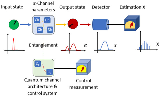
Figure 1.
Process for QPE considering a composed architecture for the channels and ruled by controls.
2.2. Cramér–Rao Bound
The classical CRB is a fundamental result in mathematical statistics establishing a lower bound on the variance of any unbiased estimator of a parameter. It provides a measure of the best achievable precision for estimating the parameter based on the available data. The bound is derived using the Fisher information, which quantifies the amount of information carried by the data about the parameter. Specifically, the CRB states that the variance of any unbiased estimator is lower-bounded by the inverse of the Fisher information. This result has significant implications for the efficiency of estimators and serves as a benchmark for evaluating the performance of different estimation methods [20]. In the theory of statistical estimation, the CRB [6] establishes the minimum possible variance for an estimator of a specific deterministic parameter drawn from its statistical distribution.
Analogously, there is a quantum version for the CRB, in this sense, QFI [4] can be obtained from the statistical distribution of the CRB indicator, setting a lower bound for the joint variance of estimation:
where N is the size of sampling in a repeated experiment and is the QFI matrix. In our following development, we will consider the analysis of the single or unitary experiment case, which means as bound.
2.3. Quantum Fisher Information Remarks and Limitations
Several remarks and limitations about QFI are suitable here, particularly in the QPE context. In the operative domain, note that QFI exhibits a non-trivial form in terms of the logarithmic derivatives from the output state carrying out the channel parameters information, thus making its dependence non-linear from . Such a fact has conditioned the extended analytical approach of QFI applications for general channels, in particular, for the CRB considered below. Despite this, some affordable expressions have been developed for special cases as previously mentioned. Moreover, the last expression particularly includes the more complete case where there exist multiple parameters characterizing the channel, which naturally increases the non-linearity [19]. In the current work, the Bloch representation for QFI being present in Pauli channels partially lets the analysis [18,19]. Despite this, in the current work, the complexity of the architecture considered, by itself introduces analytical limitations. Another important fact already noticed in QPE [21] is the discontinuous behaviour of QFI in points where the QFI matrix exhibits a rank change [22]. This issue will be noticed in the current analysis.
In another trend, we should note that QFI is a mathematical extension in the quantum domain inherited from Statistics. Thus, this approach still should deal with some quantum features not directly involved in its quantum extension. Such is the case of the limitations imposed by the Heisenberg principle: the Heisenberg limit. In fact, over the CRB, the Heisenberg limit imposes the speed at which the absolute statistical difference between two pure states in the Hilbert space (or in the space of density operators for mixed states) could change along a specified path. This fact sets in metrology an optimal rate to reach a certain accuracy of a measurement in agreement with the energy used there [23].
Also, because QFI characterizes the sensitivity of a quantum state to variations, still encompassing unitary operations, it inherently lacks invariance to general changes, which is easily expected from its non-linear construction (1) and (2). Despite this, there is evidence that entangled states can attain the Heisenberg limit [24] by reaching increased QFI values. This optimization reached by the presence of entanglement lets to resume the maximum QFI over potential local unitary operations [25]. Thus, the presence of entanglement in the metrology appears convenient in general explaining the QPE advantage exhibited by PS and ICO, inherently involving entanglement, particularly if such schemes additionally include local operations.
Then, the employment of QFI is instrumental in assessing the efficacy of probe states in metrology, revealing the dual correspondence between the increase in QFI average and the detection of entangled states [26]. Thus, in our approach, as in some former strategies, the entanglement generated by the superposition boosted by a control system supersedes the QPE based on a single channel or still a sequential chain of channels.
Finally, note that certainly all metrology processes could become accompanied by undesired noise, which is normally addressed under Quantum Error Correction (QEC) schemes [27,28]. In our approach, we have assumed that our QPE context is free of noise other than the introduced by the noisy channel under analysis, which is expected to become characterized. Nevertheless, such processes are normally included in the QPE domain, and currently, they are studied to provide approaches that also effectively deal with the Heisenberg limit [29,30].
2.4. A Brief Context of General Improved QPE Efforts
The quantum identification problem has been remarked as an important procedure in metrology [31]. In such a problem, in general, a quantum system is used to reach some properties of another quantum system. Particularly, specific systems of interest are quantum channels, systems modifying the quantum state of another probe system as a function of some of their constitutive parameters. This single problem has several complexity issues particularly due to the quantum nature of the involved systems and the physical variables being present in terms of the Heisenberg principle [5].
The depolarizing channel with arbitrarily higher dimensions has been commonly employed to try concrete strategies because it is an extreme example of a channel erasing the underlying information of any probe state, thus it is considered a limit case in channels QPE [8,32]. Of course, in those approaches, the most logical QPE implementation is based on the single arrangement of the probe state crossing the single channel under analysis. Nevertheless, it was soon discovered that other probing schemes could be identified to improve the single-channel estimation. Thus, possible alternative schemes included the re-circulating of the probe state backing on the channel several times or other identical copies of it [8], but also the entangling of the probe with another before the measurement [31,33].
More recently, the implementation of ICO arrangements has shown additional important improvements in the QPE for the depolarizing channel [34,35]. Such a diversity of efforts has stated QPE hierarchies among the more effective procedures [36]. After such communication approaches, new works have proposed more elaborated communication strategies containing the channel under analysis to improve the lower bound imposed by QFI [37], which particularly involves the use of local transformations with success. Following these last trends, and particularly using a specific approach for the theoretical treatment of ICO implementation for the entire family of Pauli channels [38], this work pursues an improved QPE procedure superseding some previous sequential, single ICO, and scaffolded PS and ICO strategies for those channels [9,21].
2.5. Pauli Channels Basic Preliminaries
Pauli channels are a class of quantum channels used to describe the effects of noise and decoherence on quantum systems. Because a quantum channel should reflect the multiple scenarios that a quantum system could transit on time, it is represented as a decoherent operation performed on a certain arbitrary input state (pure or mixed). The Kraus representation comprises those kinds of operations [39]. For two-level systems, Kraus operators could be expressed in terms of Pauli operators. Moreover, under a proper basis change, Kraus operators become proportional to each Pauli operator through certain coefficients [38], a set of four parameters depicting how each channel becomes an incoherent mixture of basic operations of syndromes precisely depicted by the Pauli operators (the invariant or transparent operation , and the other three syndromes on qubits: bit-flipping, dephasing-noise, and a combination of both).
Thus, Pauli channels are defined algebraically using the Pauli matrices, a set of four matrices including the identity matrix () and the three Pauli matrices ( and ). The algebraic representation of Pauli channels allows a concise and convenient framework to analyze various noise processes in quantum systems [40]. Pauli channels find diverse applications in the field of quantum information theory. They are primarily used to model and study the effects of noise and decoherence on quantum systems. These channels play a crucial role in understanding the robustness and stability of quantum information processing tasks, such as quantum computation and quantum communication, in realistic noisy environments. The general depiction of Pauli channels can be written as:
where are the Pauli operators with , is the identity operator and are the Kraus operators [39] with . Note, from (4) that and therefore . In this case, the parameters are the ones that will characterize the type of channel. By expressing the Bloch density matrix in terms of the Pauli operators (which are precisely the same Kraus operators in the channel) , we can represent the state of a qubit using just three real parameters (the coefficients associated with the Pauli matrices). This representation is highly compact allowing an easier manipulation of the quantum state. The entire family of Pauli channels has been represented in a tetrahedron space as the Pauli Channels Parametric Space [38] (PCPS).
2.6. Improved Circuits to Reach More Optimal QPE
ICO arrangements have been proposed as experimental methods because they have been shown to improve quantum communication [41,42,43], where other different treatments have been developed to analyze them [44]. ICO is a concept that has been studied in quantum channels for a variety of applications. In [45,46], a study of the use of superposition of causal orders in quantum teleportation was presented for very noisy channels, showing that the use of superposition of causal orders can lead to a significant improvement in the fidelity of teleportation under very noisy channels. In [47], the use of superposition of orders is applied in quantum communication, where the use of superposition of orders can increase the communication capacity of a quantum channel. It is demonstrated that the use of indefinite causal order can lead to a significant reduction in the amount of entanglement required for quantum communication [41]. In the experimental field, it is presented an experimental realization of a quantum switch that can be in a superposition of two different orders of gates [43]. There, it has been shown that such a switch can be used to implement a quantum algorithm with a quadratic speedup over classical algorithms. They also demonstrate that such a switch can be used to implement a quantum error correction code more efficiently than the best-known classical code. While [48] presents an experimental realization of a quantum switch that can be in a superposition of two different orders of gates. By leveraging ICO, quantum communication protocols could experience unprecedented advancements. Thus, by using higher orders under ICO than the switch, the communication performance has been used to analyze the Pauli channels [38]. The ICO arrangements, then, have remarkable properties for improving communication. However, in the case of QPE, the capabilities of these arrangements have shown limited outcomes [9,21].
On the other hand, the PS of quantum channels has several important applications in quantum communication. One of the key applications is using trajectories as a quantum control to rule the order of noisy communication channels. This quantum control has been shown to enable the transmission of information even when traditional communication protocols through well-defined trajectories fail [49]. The use of channels in series with quantum-controlled operations within the framework of quantum interferometry has been found to yield the largest advantages, allowing both the information exchanged and the trajectory of information carriers to be quantum, which has been demonstrated experimentally and numerically in quantum-optical scenarios [49]. Furthermore, by considering superpositions of alternative evolutions or orders, quantum particles can experience interference effects, leading to cleaner communication channels and boosted capacity to communicate classical and quantum bits [41]. Experimental demonstrations have shown the communication advantages of superposing alternative channel configurations. These applications represent the potential of PS in enhancing various aspects of quantum communication and furthering the understanding of quantum Shannon theory [50].
Summarizing, channels’ parameters determine the effect of each specific channel on a quantum probe state, and the process can be enhanced using different composed architectures as coherent [51,52] such as sequential combinations, superposition of channel paths, and even ICO [9]. The use of ICO and PS opens up more possibilities for QPE. By exploiting both concepts simultaneously, researchers have demonstrated the potential to surpass classical limits.
3. Architectures Involving Copies of a Quantum Channel and Additional Quantum Controls
3.1. Kraus Representation for a Combined Architecture of Channels Involving Controls
Some architectures of channel arrangements have been proposed in the context of quantum circuits architecture, in particular, for QPE to improve the parameter estimation. In the present analysis, we propose the use of a general architecture consisting of a combination of the best previous analysis of channel arrangements. In this case, the architecture is considered for the Pauli channels family.
Certain combinations of identical channels appear more convenient for QPE as sequential or other implementing ICO [9]. Moreover, the proposal of certain circuits involving additional control operations together with those combinations [19] has become useful to state performance hierarchies among those arrangements for QPE. In particular, the use of PS and ICO as composed architectures including other control operations has shown notable advantages on the single use of those causal order arrangements [21]. In the last work, specific PS and ICO architectures with controls demonstrated dramatic improvements in the lower bounds of QPE. Thus, in the current analysis, the coherent combination of those architectures is studied trying to reach better outcomes.
In this article, we look to unify path superposition and ICO together with other strategies such as entangled test states to increase the estimation efficiency. With ICO, by carefully choosing the order of measurements and operations, it is possible to minimize the resources required for parameter estimation, leading to higher estimation efficiency [53]. Additionally, ICO and PS can offer robustness against noise and imperfections, making quantum parameter estimation more resilient to environmental disturbances and experimental imperfections [54].
Considering the general form for the Kraus operators for Pauli channels as follows:
with while . are the structure constants for the circuit involving the single channel whose parameters are pretended to become estimated [21] (here, we are considering a couple of controls instead of the only one included in that reference). In the following, for simplicity, Latin scripts run on , while the Greek ones run on . The subscript 0 corresponds to the system (probe state) going through the architecture arrangement and subscripts and refer to the controls on the scheme to select the different configurations. These Kraus operators should fulfill the condition , and therefore:
Using the Bloch representation for the input state , where we have extended the three-dimensional Bloch vector ( ) into the four-dimensional one . Particularly, it is possible to parametrize in terms of a pair of angles as . Similarly, , the identity and the Pauli operators. In such expressions, as traditionally. The output state could be written as:
which implicitly includes the control system in . There, by writing in terms of :
there, are the entries of . In addition, because:
then, we get:
the component of expanded in a linear combination of . It also includes the control systems, which are in general entangled with the state going through the channel arrangement.
The output state is a composite state including the controls, and therefore, it does not directly admit a Bloch representation. In such cases, there are two alternatives if one desires to obtain a state admitting a Bloch representation. One option is to consider an analysis that disregards the controls by partially tracing out those unwanted states. The other option is to measure the controls, which involves a stochastic process, waiting to obtain certain states that are more suitable for parameter estimation. By doing the tracing process, the focus is placed solely on the desired probe state that can be represented using the Bloch representation. This approach simplifies the analysis by disregarding the control components and allows a more straightforward parameter estimation process. On the other hand, by measuring the controls of the system, it is introduced a stochastic process where the measurement outcomes of the control systems are utilized to obtain certain states that are more favourable for parameter estimation. This approach relies on the measurement results of the control systems to select the test state, potentially improving the accuracy and precision of parameter estimation.
3.2. Output State for the Tracing Out or the Measuring of the Control States
Thus, by tracing the control systems and using the property (6), it is possible to demonstrate that for the tracing out (T) adopts the mixed state form for a single qubit system ():
thus providing an expression for which can be inserted in (2). Unfortunately, tracing will imply in the practice repeating the measurement of both controls several times on the bases , to reach an averaged .
Otherwise, by optimally measuring the control states using a privileged basis for each one: ; for instance, and . Then, when and are measured the output state obtained after the controls measuring (M) becomes:
there, is the probability of success to obtain and :
clearly it implies . In the following, the measurement bases will be written as:
which states a set of particular cases because coefficients are considered real. In the following discussion, we will assume that the optimized solution is represented by , having a success probability . Consequently, our QPE process will become stochastic. In addition, its optimization analysis involves the two additional selectable parameters and , which will represent a more complex computational effort. In general, for the T and M cases, those approaches simplify the mathematical challenges involved in QPE by allowing the global state to return into a form that can be expressed using the Bloch representation, thus easing the QFI calculation as in (2).
4. Proposed Architecture for the Improvement of QPE Controlling the Symmetry Balance of Superposition between Two Communication Strategies
In the current analysis, we study the QPE problem for an unknown Pauli channel (). The channel is involved in a quantum circuit containing several copies of it. In addition, those copies are connected following emblematic communication connections as ICO and/or PS [37]. This process is depicted in Figure 2, representing with and the index for the single Kraus operators of each one of the two channels involved. Those copies are connected in superposition under a pair of causal structures: Paths superposition and ICO. Thus, one control , assumed in the state , decides the type of causal structure, path superposition (green, ) or ICO (blue, ). Together, the control in the state defines the path order or the causal order, beginning with the upper channel (, solid lines) or the lower one (, dashed lines). An additional unitary control gate U is included to improve the QPE. This last gate is alternated for path superposition or lays in the middle for ICO, summarizing the structures considered in [21] separately.
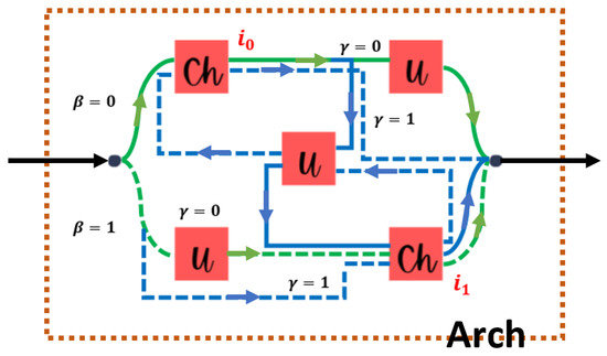
Figure 2.
Proposed architecture for QPE involving two copies of a quantum channel and a unitary operation . A couple of controls will rule the path followed () and the causal structure: Path superposition (green, ) or ICO (blue, ).
Regarding the last figure, the mathematical expression for the structure constants becomes:
the coefficient is due to the normalization of Kraus operators for each causal structure as in [21]. In the current analysis, we will assume the probe pure state (it means ). In addition, considering with , then, the optimization problem, considering the controls’ states measurement scheme (M) to get the minimum bound for should consider the swept on the set of nine selectable parameters: , with and .
The procedure to get requires the use of Formulas (15) and (16) in combination with (19) to get in . Thus, getting the Fisher information matrix, its eigenvalues could be found (as instance with the procedure depicted in [55]) to finally arrive at the expression of . Nevertheless, expressions for are large and complicated for the proposed architecture, so at this point a numerical procedure is more convenient for substituting the selectable parameters’ values, obtaining the derivatives numerically. For those reasons, a method such as the Monte Carlo one should be preferred to reach the optimal values.
To illustrate this fact, we have obtained for the uniparametric sub-family of Pauli channels characterized by and (it was still calculated under the multiparametric approach for those channels), considering a random sample of size sets of selectable parameters on to numerically reach the statistical distribution for . Values of were grouped on 25 subsets of equal size on the obtained data range. The outcomes are shown in Figure 3 for (A) , (B) , (C) , (D) , (E) , (F) , (G) . Red dots correspond to the class mark and the black solid line is a spline fitting of order 6. Each plot is limited to the obtained data range in each case and then represented in the same interval to ease the comparison. Note, for , that the peak of the distribution is displaced on the right respect to those cases for . Although the sample could not contain the lowest possible values, this analysis shows the expected behaviour, the presence of values near zero drops to zero dramatically for .
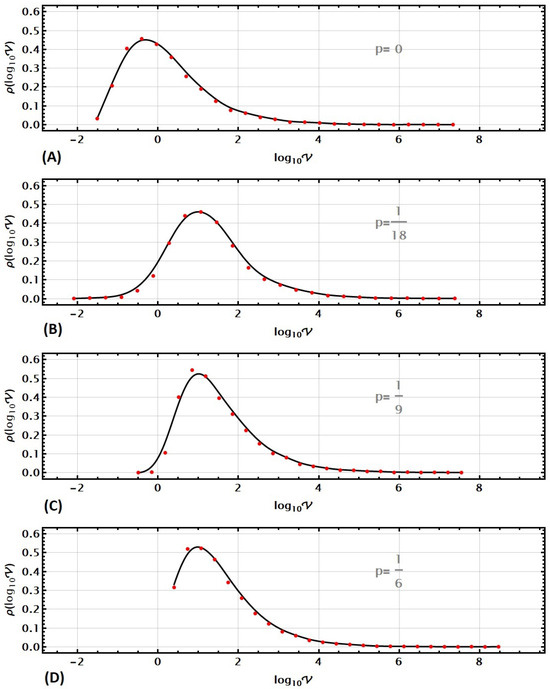
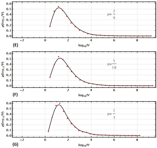
Figure 3.
Statistical distributions for obtained numerically using a sample of size on for (A) , (B) , (C) , (D) , (E) , (F) , (G) .
5. Analysis and General Outcomes for QPE
Previous outcomes in QPE reported in the literature for Pauli channels have used several types of combined architectures using unitary control gates [21]. Thus, common architectures involving PS (named PS+U and PSA+U) have demonstrated the best minimum values . Despite this, still ICO architectures give the best outcomes for a limited subset of Pauli channels. In this section, we analyze the proposed architecture (ICO-PSA+U) for QPE purposes as compared with the previous best outcomes for .
5.1. Bound for the Parameter Estimation through Several Emblematic Pauli Channels
Because the analysis to find involves nine parameters through , the computational effort supersedes the effort being present in [21]. Thus, we analyze the QPE outcomes for a representative set of Pauli channels characterized by . They include the transparent, the depolarizing, and the central-ICO channels [38], some emblematic Pauli channels. Note, that despite apparently a single parameter being considered, we are performing the analysis on the multiparametric domain for the states surrounding this line on the three-dimensional parametric space of Pauli-channels. We used a Monte Carlo method on resizeable regions through . Despite this, our effort implied to improve the first obtained outcomes to discriminate between possible local minima. The final outcomes have been reported in Figure 4 including a comparison with the best previous outcomes [21] reporting simpler architectures using PS and ICO, one at a time.
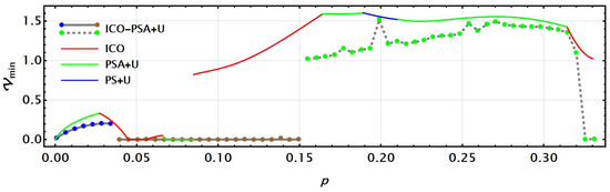
Figure 4.
Best bounds for found through the central line in the Pauli channels parametric space as a function of p for the proposed architecture, ICO-PSA+U (solid and dashed grey lines), compared with the previous best outcomes using other architectures (PS+U -blue-, PSA+U -green-, and ICO -red-).
Solid lines report the best outcomes in [21] using ICO (red), PSA+U (green), or PS+U (blue) architectures independently for each p-value. Then, the outcomes corresponding to ICO-PSA+U architecture are reported with a grey line (solid or dashed). They include the improved values for the set of p-values analyzed marked with dots (in blue, brown, and green for convenience). Results show the expected improved outcomes obtained by combining the leading architectures ICO and PSA+U in a coherent superposition. Several aspects presented regarding the optimal values should be noted. The central region with (brown dots) exhibits the best outcomes for between , then almost unnoticeable in the plot. Otherwise, values in the region with (blue dots) comprise values below pure PSA+U and ICO architecture in a well-defined curve with values below . In these two last cases, our procedure was able to find multiple solutions for the minimum values of , in agreement with the distribution outcomes presented in Figure 3 for those values of p.
Finally, the region characterized by has the largest values but, of course, below the single architecture cases on an apparent irregular curve for that reason represented by a dashed grey line. The peaks with larger values for through the curve represent hard p values for the optimization of the bound, just finding the reported values after repeated improvements by our numerical procedure. Thus, those outcomes are obtained and reported on the limit of our numerical procedure. In fact, most of the numerical procedures to reach the minimum value of (and the set of optimal selectable parameters in ) in were delayed around six hours each on a -core computer checked successfully at least twice. Instead, for the region , each channel calculation required multiple checks to report the optimal value found. For the elusive peaks around and , the procedure was repeated more than 20 times each to reach the best outcome reported in the plot. Then, because the global behaviour of the optimal solutions suggests being multiple, for those two peaks the solutions appeared concentrated in smaller regions hardening the search. It suggests a change in the continuity of QFI reported in the literature [22], which unavoidably depends on the architecture being considered and its complexity as it is in this case. Of particular interest, is the peak in which practically reaches the value for the previous outcome reported for the PS+U case, which locally becomes better than PSA+U one in such region (blue line). Note, that the PS+U strategy is not obtained as a reduction with the ICO-PSA+U architecture being proposed (just the PSA+U one), being that the main operative reason for this peak, but still resting on a deeper property for that narrow group of channels already noticed in [21] where PS+U architecture dominates.
In addition, the sudden drop to zero of near the central-ICO channel (note the consistency with the peak in Figure 3G where a tiny recoil is observed). Such outcomes exhibit discontinuities among them as the outcomes presented in [21]. In general, it is possible to notice a clear consistency of those last outcomes with the statistical distribution for , setting the difficulty to reach numerically the optimal values for .
As it was stated in [21], the optimization of on commonly includes multiple solutions. By analyzing the prescriptions for the selectable parameters in the solutions presented in Figure 4, such an aspect is also verified in the current case, thus, the solutions there may not exhibit a defined behaviour in some of those parameters. Nevertheless, still some analyses were included here. Figure 5A compares and for the overall set of solutions in Figure 4. It shows, in addition, the value of p in colour, in agreement with the colour bar at the bottom, thus making reference to Figure 4. While in the cases reported in [21], there was a remarked correlation between this pair of parameters, in the current case it is just limited to the best-defined group of solutions for (red dots) establishing the linear correlation also observed in [21]. For the intermediate values of p (green dots), the almost perfect values appear located in the plot borders or , indicating a preferred path since the beginning in the control state or post-measuring. Larger values for p appear dispersed without an apparent correlation.
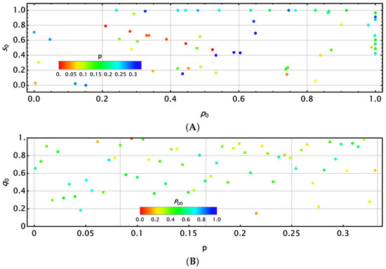
Figure 5.
Some notable relations among selectable parameters in the optimal QPE configuration. (A) Between (path or causal order superposition) and (path or causal order control measurement), as a function of p in colour and (B) between (causal structure superposition) and p (type of channel), reporting the success probability for the best stochastic controls’ measurement (in colour).
In another view, Figure 5B compares p versus in colour but still includes the values of success. A clear recurrence for large values becomes evident in the plot, thus preferring the PS component in the superposition. This aspect is in general expected from the outcomes in [21]. In addition, the colours remark satisfactory values for centred near (green). This plot also shows that increases with the value of p (PS preferred on ICO in the superposition).
5.2. Bound for the Parameter Estimation near Syndromic Pauli Channels
In this subsection, we analyze the QPE outcomes for those Pauli channels near the pure syndromic channels: Bit-flipping (), Dephasing noise (), and their combination: (). First, we have obtained for each of those channels regarding a random sample of size sets of selectable parameters on to numerically reach an approximation to the statistical distribution for , following the same previous procedure using a spline fitting of order 6.
The outcomes are shown in Figure 6 for (A) Bit-flipping channel, (B) Bit-flipping + Dephasing noise channel, and (C) Dephasing noise channel. Each plot is limited to the obtained data range in each case and then represented in the same interval to ease the comparison. Note, that the peak of the distribution in all three cases is around zero (with a little displacement on the left and a narrower distribution for the dephasing-noise case). Thus, we expect better results for QPE near those syndromic Pauli channels, at least as compared with the channels on the central line in Figure 3, where the peak distribution is always on the left side of , thus expecting to obtain pretty small values for .
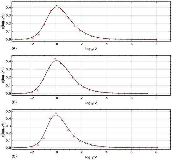
Figure 6.
Statistical distributions for obtained numerically using a sample of size on for (A) Bit-flipping channel, (B) Bit-flipping + Dephasing-noise channel, (C) Dephasing-noise channel.
Following the analysis for the syndromes for Pauli channels as in [21], we will analyze the case for the corner of the Pauli channels parameter space [38] characterized by near from each channel syndrome i (Bit-flipping noise , Dephasing noise , and their combination ). By considering a uniform sample of channels in that corner region for the considered architecture, we obtained an insight into the behaviour. Outcomes are shown in Figure 7 together for the three syndromes.
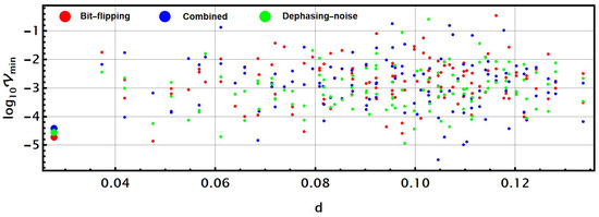
Figure 7.
Best bounds for for the proposed architecture found for a sample of channels nearest () to each syndrome channel () in each corner of the parametric space of parameters. They are shown as a function of their distance d to the specific syndrome: Bit-flipping (red), Dephasing-noise (green), and combined (blue).
Outcomes for are similar for the three syndromes. They are shown in a different colour for each syndrome: Bit-flipping (red, ), Dephasing-noise (green, ), and the combined (blue, ). Each dot represents the outcome for a channel uniformly located in the region with as a function of its Euclidean distance to the exact syndrome as measured on the Pauli channels parameter space. For the dephasing-noise case, no apparent difference explicitly appears as could be expected from Figure 6C. Critical values on each syndrome are represented with the biggest dots on the left. Differences among them could become non-meaningful as an effect of the scale, they are in the precision limit of our numerical calculation. In any case, those outcomes reflect an excellent possibility of the QPE problem of those three channels.
6. Alternative Scaffolding Strategies for the Architecture in QPE
Some other strategies have been proven to improve QPE. The construction of a specific circuit involving the channel under analysis together with complementary control operations (as U in the proposal being analyzed) is not the only strategy. Otherwise, the use of entangled probe states has been considered in the literature [8,37] with notable advantages for maximally entangled probe states, particularly for the case when just one of the subsystems goes through the QPE preparation [8], although those outcomes were proved for the depolarizing channel. In some sense, if just one of the subsystems goes through the preparation, it suggests that certain interference between the input state and the exposed one to the channel becomes profitable. Alternatively, we could compare such a strategy with an additional PS using the architecture and not using it. This communication effect could be reached by implementing double teleportation [56] by replicating the input state in a pair of superposed copies ruled by a control state. Then, just one of such copies is exposed to the QPE architecture in comparison with the previous scheme using a probe entangled state.
Both arrangements are shown in Figure 8 exhibiting the entire architecture circuit inside an orange dashed box. Figure 8A shows the teleportation control system sending to two parties, one of which applies the architecture while the second does not. The outputs in each party are again coherently deposited in just one, becoming indexed by the control state as a unique output for the QPE process. Figure 8B shows a bipartite state on systems a and b, possibly entangled, being modified by the architecture in only one of their parties (a). Inside each box are the additional controls and of the architecture (not shown in the plot). At the end of both processes, a measurement for the teleportation control or in the party b are, respectively, performed to leave a single qubit state to be analyzed under the Bloch representation approach for the QFI.
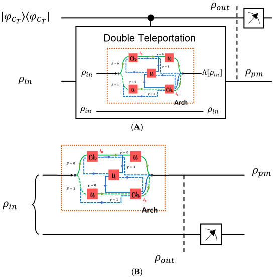
Figure 8.
(A) Controlled double teleportation where only one of the receivers apply the architecture for QPE, and (B) Bipartite probe state where only the first party apply the architecture for QPE.
6.1. Double Teleportation as an Additional PS Strategy in QPE of Pauli Channels
Double teleportation, as it was introduced in [56], first considers the state to be teleported to a pair of parties receiving copies of it in superposition in agreement with a control state . Then, each party coherently applies independent operations on its copy to finally close them together over one of them using a SWAP gate. The teleported and processed states are then allocated in party a as an instance, it becomes:
In the current case, is the identity, while is in fact the architecture arrangement (see Figure 8A), which is not a coherent operation, so the outcome is in fact:
where could be considered in the tracing (T) or in the measuring (M) strategies in agreement with the expressions (12) and (14), respectively. In any of those cases, no entanglement is already exhibited in both subsystems, control of teleportation and qubit a. Entanglement in the previous subsystems a and b has been transformed in a superposition of both outcomes deposited on subsystem a. Any advantage for QPE will be considered a measurement on a different basis that is stated by the states of the teleportation control subsystem. As an instance, considering the measuring basis for the teleportation control and assuming the first element as the optimized element to improve , then, the post-measurement state becomes:
this expression lets calculate the QFI from (2). is the success probability of reaching the correct measurement on the teleportation control. There, is obtained from our previous basic approach just considering (13) or (15) as a function of the strategy followed, (T) or (M). In the more complex scheme, (M), which will be followed in the further development, the selectable parameters increase in two, : , with and .
The procedure to get requires the use of the formula (23) to reach the expression for to feed (2). There, a numerical procedure has been applied by substituting the selectable parameters’ values, then obtaining the derivatives numerically, thus obtaining . By considering a random sample of size sets of selectable parameters on , we numerically reached an approximation for the statistical distribution of as in the previous cases. The outcomes are shown in Figure 9 for (A) , (B) , (C) , and (D) , using spline fittings of order , respectively. Each plot is limited to the obtained data range in each case and represented with an appropriate scale to show the entire results. Note, that the peak for all the distributions is located approximately at the same value . Moreover, comparing the outcomes of Figure 3, we notice a wider distribution slightly displaced to the right, showing that the additional strategy worsens the possible outcomes in general. Still, it is clear that our previous strategy in Section 5 is contained here if just the upper path in Figure 8 is considered (). Still, we bet on the possibility that better values for could be reached.
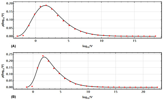
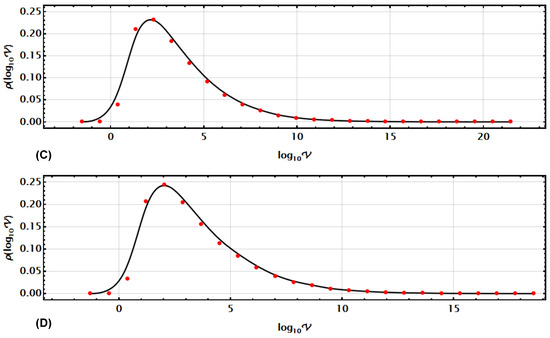
Figure 9.
Statistical distributions for corresponding to the architecture involved in a double teleportation is just one of the paths. It was obtained numerically using a random sample of points with a size of on for (A) , (B) , (C) , (D) .
6.2. Entanglement States as Probe States in QPE of Pauli Channels
The use of entangled states as probe states has been shown to offer substantial improvements in quantum parameter estimation processes. The family of parallel strategies stands as the pioneering and notably successful instance of quantum-enhanced metrology, demonstrating the utilization of entanglement to achieve a precision surpassing classical limitations. This concept has been explored in various studies, showcasing the advantages of using entangled probe states. For instance, in the context of estimating the phase of a unitary transformation on a qubit affected by depolarizing noise, entangled qubit pairs have demonstrated enhancements in performance compared to separable probe states [57]. Even when one of the entangled qubits does not interact with the process being estimated, the presence of entanglement leads to improved performance. This enhancement holds for both partially and maximally entangled qubit pairs, depending on the level of noise [58]. Another example, in the context of quantum metrology, several strategies including independent channels, sequential channels, or channels in parallel using a general entangled state and superposition of causal order have been probed, where those strategies provide no asymptotic advantage over the case where an entangled probe state has been used [11]. Similarly, Ref. [37] establishes a structured framework for discerning the ultimate boundary of precision for various categories of approaches, including parallel, sequential, and indefinite causal order tactics and proving an algorithm for selecting the most suitable strategy within the specific category, positioning the parallel strategies with the use of entangled states as the pioneer in improving parameter estimation.
In agreement with the development included in the Appendix A, a bipartite state on qubits a and b can be written in terms of a matrix as:
with as before. Thus, if the architecture is just implemented on party a (see Figure 8B):
where could easily be obtained from (13):
for the tracing (T) strategy, and:
for the measuring (M) strategy obtained directly from (15). As before, the success probability for the QPE process is assumed to be .
Also, as in the previous double teleportation strategy, a joint non-local measurement between the subsystem bases is expected to gain an advantage for QPE. Thus, in the following, we will consider the following bipartite state as the initial probe state (with real coefficients) [59]:
this proposal, despite not being general, already introduces an additional parameter in comparison with the previous approaches regarding single probe states. With this expression, we can construct a definite form for matrix . In fact, it requires writing , then projecting it into the basis to reach the entries. They are reported in the Appendix B in (A8). Note, that the expression (25) is valuable because it splits the initial state information stored in from the generic effect of the architecture, .
Finally, if the subsystem b is measured in the basis and assuming the first element as the optimized element to improve , then the post-measurement state and the measurement success probability become:
be aware of the nature of those expressions. is a four-component vector whose entries are operators obtained as a linear combination of Pauli matrices and the identity. In , such a four-component vector becomes multiplied by on the right, while the expression is multiplied on the left by the four-component vector of scalars given as , the expectation value of under the state . It gives the operator . More concretely, for the QFI calculation using the formula (2):
For the more complex scheme, (M), the selectable parameters increase in two by replacing with , and introducing : , with [59], and . We will follow this approach (M) in the following.
By repeating the previous procedure of obtaining with (32) to reach and then feeding (2), we finally used the same numerical procedure. The selectable parameters’ values were substituted, then reaching numerically values. First, we again get a numerical approximation for the statistical distribution of through a random sample of size sets of selectable parameters on under the same previous methodology. The outcomes are shown in Figure 10 for (A) , (B) , (C) , and (D) , implementing a spline fitting of order , respectively. In this case, the peak is located at lower values than the teleportation strategy, between 1 and 2 with the transparent channel () as an exception, below 0. All of them become narrower distributions than the teleportation case, barely similar to the original strategy with the architecture alone in Figure 3. Despite this strategy contains in principle the original one in Section 5, we have entirely limited our analysis to the authentic probe entangled states, thus avoiding the separable states (in the frontiers or , or ) [59].
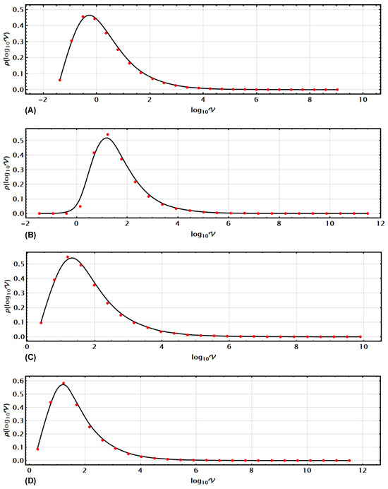
Figure 10.
Statistical distributions for corresponding to the architecture using entangled states as probe states. It was obtained numerically using a random sample of points with a size of on for (A) , (B) , (C) , (D) .
6.3. Bound for the Parameter Estimation for Pauli Channels Using the Architecture under PS or with Entangled Probe States
To reach , the Monte Carlo method has been applied on and as previously depicted in Section 5. Thus, we have obtained for the uniparametric sub-family of Pauli channels with and . We have limited our analysis to the still imperfect regions obtained in Section 5, and , looking for better values for in these regions. Outcomes are shown in Figure 11.
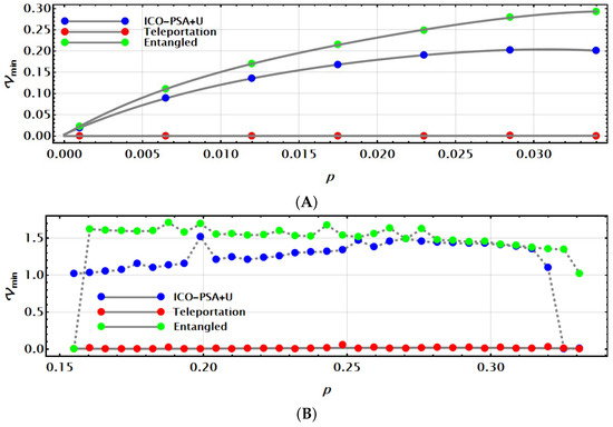
Figure 11.
Best bounds for found through the central line in the regions (A) , and (B) . Red dots show the case scaffolded by the PS strategy using double teleportation, while green dots represent the case where strictly entangled probe states are used. Blue dots are the corresponding outcome in Figure 4 with the single use of the architecture.
Thus, Figure 11A presents the outcomes for the PS support implementing double teleportation (red dots) and entangled probe states (green dots) for . Blue dots show the same outcome for this region already reported in Figure 4. A notable outcome is obtained using PS, reaching . Despite this, the outcome using entangled states becomes worse than the single use of the architecture with single probe states.
Instead, Figure 11B shows the outcomes for the region . Again, the PS case reached with the use of double teleportation exhibits notable outcomes with (red dots). But as before, the use of entangled states does not report improved outcomes (green dots) in comparison with the single use of the architecture (blue dots).
6.4. A Final Summary for Quantum Sensing in Quantum Parameter Estimation for Pauli Channels
The QPE problem for Pauli channels has been addressed through several approaches, each one superseding limitations in the lower bound as stated by the Cramér–Rao bound for the joint variance for the estimation of each one of the free parameters involved in their characterization . The first approach is the direct use of a specific Pauli channel or a train of copies from it arranged sequentially (SEQ) [9]. The outcomes are mild because the bound for becomes above the unity considering that the parameters being estimated are lower than one [9].
The employment of some communication schemes where copies of the same Pauli channel analyzed are included, ICO for instance, provides only limited improved outcomes for the bound just for certain channels, as the Central ICO one, but surprisingly conducts to worse outcomes for those channels where the sequential strategy provides better values for . In any case, the crucial value is limitedly superseded. The proposal of local unitary operations included in the design of the previous strategies has provided better outcomes at least for schemes such as ICO (ICO + U) or PS (PS + U or PSA + U), but not for the sequential approach (SEQ + U) [21].
Thus, these unitaries with their selectable design parameters to improve the QPE outcomes move dramatically the previous schemes lowering the bound below , at least for the transparent channel and for the pure syndromic channels. Those schemes or architectures set the bound near to zero, but not in general. In our current architecture combining two of the best schemes (PS and ICO: ICO + PSA + U), still considering the support unitaries, the outcomes dramatically improve, with only a few regions being partially reluctant but clearly below the single previous communication architectures including unitaries.
For our last approach, we include other ideas already proposed in the literature as the use of entangled probe states [11] or still a second PS strategy, in both cases combining the outcomes for the proposed architecture with the original single probe state to boost the destructive interference of some components increasing the bound. Finally, our strategy using a second-order PS implementation with our original circuit proposed (PS + (PS + ICO + U)), lowers the bound to zero in the remaining regions. Despite not the generality of channels having been analyzed, this strategy works for a family of representative Pauli channels. Tracking of the last hierarchies found for the last approaches is synthetically depicted in Figure 12.
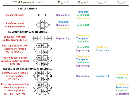
Figure 12.
A summary of hierarchies for the lower bound of for the multiparametric case, comparing several types of Pauli channels and QPE approaches.
7. Conclusions
In the present work, we established an analytical approach to improve QPE for Pauli channels. The current method proposes combining several copies of one specific Pauli channel within a quantum circuit. Those copies were connected following the well-known communication setups of ICO and PS in superposition, additionally including supplementary local control operations inside of a structured arrangement or architecture. That arrangement incorporates extra adjustable and selectable parameters that are not the focus of our QPE analysis; rather, they were optimally chosen to enhance the QPE results. Therefore, the proposed architecture involves parallel pathways and indeterminate causal frameworks with scaffolding local operations within these structures (see Figure 2).
The analysis performed combined analytical and numerical approaches to obtain a joint lower bound for as stated by the CRB. Thus, a representative uniparametric sub-family of Pauli channels, given by and , was first considered on the entire family of those channels. Such channels include the transparent, the depolarizing, and the central ICO (the best-corrected channel by ICO) channels, together with many others combining the main syndromes. As a strategy, we first analyze the distribution of on , their complete space of selectable parameters in the architecture by considering random samples of size . Such distributions along several values of p exhibited the expected behaviour for the lower bound , an increment of it as p increases.
Then, the optimization for our central analysis was made through a Monte Carlo search procedure by considering random samples for the selectable parameters of size in each recursive approximation on resizeable regions. The outcomes showed that optimal values for the lower bound drop to zero dramatically for [21], thus delivering perfect outcomes for QPE. The nearest regions to the transparent channel in exhibited improved outcomes compared with the previous outcomes not considering the current combined architecture [21] but not necessarily dropping to zero in general. The worst outcomes (but still improved) appeared in the remaining region for , having erratic behaviour at our precision level, but better than the separate strategies (PS and ICO).
When the proposed architecture is also tested with some emblematic Pauli channels (the transparent, the depolarizing, and the central-ICO channels), it was found that improved outcomes were obtained by combining the leading architectures ICO and PSA+U in a coherent superposition, in comparison to those results found in [21] (see Figure 4). When the architecture was tested near syndromic Pauli channels (Bit-flipping, Dephasing noise and the combination of both), it was obvious that the peak of the statistical distribution for all in all three cases was around zero (one for ). Despite this, the outcomes for the lower bound fall at the same level as the practically perfect outcomes found for the PSA+U strategy in [21].
By revisiting the problem for the reluctant regions , the entire same architecture was now tested first using double teleportation, a superposition between the schemes using the architecture or not. Then, a second strategy was proved using a probe-entangled state, with just one of the subsystems going through the preparation. The analysis was made following the same previous searching procedure to reach the optimal value on their new respective selectable parameter spaces, or . Such nested strategies to the architecture gave notable outcomes. Again, a first insight was made using the distributions. In both cases, they showed an increase in the values, which suggests in general worse outcomes when an arbitrary selection of parameters is made. For the double teleportation strategy, the peak distributions were approximately located at , with a wider distribution displaced to the right. Whereas, the strategy involving entangled probe states showed peaks located at lower values and narrower distributions than the teleportation strategy. Finally, was obtained for both strategies in the reluctant regions, pointing out a disrupting outcome as compared with our insight. When using double teleportation, in both regions despite its wider distributions. Instead, the use of probe entangled states (strictly restricted to non-separable states) yields worse outcomes compared to employing the architecture with single probe states (see Figure 11).
In summary, our current outcomes have demonstrated that strategies immersing probe Pauli channels inside circuits implementing combined communication schemes between PS and ICO, particularly scaffolded by a local operation in the midway, provide notable improvements for QPE. Note, that such local operation is specific for each architecture and concrete channel because QFI is inclusively sensitive to any local variation. Nonetheless, in our analysis, such local operations still form sets of equivalent operations providing the same optimal value. This set, in our numerical analysis, appears more or less elusive under the Monte Carlo search as a function of the channel (p-value), thus denoting its density or accumulation (see the analysis performed in that direction in [21]), which deserves more future work. In the road, the approach to write composed circuits or architectures to model the QPE through their structure constants as , have contributed to the analysis in the field [21]. Such constructions should sometimes still be combined again with the original probe state to reach the optimal superposition and achieve a perfect parameter estimation inclusively implementing intelligent and post-quantum scenarios [60]. Still, in each case, the confirmation of the perfect bound for QPE just opens the research to design the experimental scheme for reaching the elusive channel characterization [61,62]. In such a search, other restrictions imposed by the quantum nature of the systems and tentative measurements should be overcome [9,63].
Author Contributions
Conceptualization, F.D.; methodology, F.D.; software, C.C.-I.; validation, C.C.-I.; formal analysis, F.D. and C.C.-I.; investigation, C.C.-I.; resources, F.D. and C.C.-I.; data curation, C.C.-I.; writing—original draft preparation, C.C.-I.; writing—review and editing, C.C.-I., F.D.; visualization, F.D. and C.C.-I.; supervision, F.D.; project administration, C.C.-I.; funding acquisition, F.D. and C.C.-I. All authors have read and agreed to the published version of the manuscript.
Funding
This research received no external funding.
Data Availability Statement
The data presented in this study are available in article.
Acknowledgments
Authors acknowledge the economic support to publish this article to the School of Engineering and Science from Tecnologico de Monterrey. Carlos Cardoso-Isidoro and Francisco Delgado also acknowledge the support of CONHACYT.
Conflicts of Interest
The authors declare no conflict of interest.
Abbreviations
The following abbreviations are used in this manuscript:
| CRB | Cramér–Rao Bound |
| ICO | Indefinite Causal Order |
| PCPS | Pauli Channels Parametric Space |
| PS | Path Superposition |
| QEC | Quantum Error Correction |
| QFI | Quantum Fisher Information |
| QPE | Quantum Parameter Estimation |
| SEQ | Sequential |
| U | Unitary operation |
Appendix A. Bloch Representation of Bipartite States
A pair of possibly entangled states could still be represented in a Bloch-like representation. If are the traceless generators [64], together with as the identity matrix, then, any bipartite state constructed by a system of dimension N and other of dimension M could be expressed as [65]:
by demanding that then . Additionally, considering the partial trace concerning each subsystem:
Thus, by noting in each case that for pure states , and associating a Bloch unitary vector for those states, in this case, it is necessary that and [66]. Similarly, for pure separable bipartite states , then it is possible to demonstrate that for those states:
then, in general we define a normalized quantity , reaching the value of 1 in that case (separable pure states), . Thus, for the general case:
being . The last sum, for the pure separable states case, will become , then . It directly implies that and . Moreover, the last expression could be written more synthetically by defining and the matrix :
being the matrix defined above. Then:
Finally, note that for a couple of qubits, . In this case, the matrix has some interesting features. By writing for a pure state as , a direct calculation shows that , which reflects the symmetry of the states for the two parties, particularly reached for . Also, , the state concurrence , becoming zero for separable states and one for maximally entangled ones).
Appendix B. Parameterized Matrix D for a Bipartite State with Real Coefficients
If a pure bipartite state in the form of (29) is considered, then, the non-zero entries of matrix for the corresponding , become:
Notably, .
References
- Baamara, Y.; Gessner, M.; Sinatra, A. Quantum-enhanced multiparameter estimation and compressed sensing of a field. SciPost Phys. 2023, 14, 14. [Google Scholar] [CrossRef]
- Ikken, N.; Slaoui, A.; Ahl Laamara, R. Bidirectional quantum teleportation of even and odd coherent states through the multipartite Glauber coherent state: Theory and implementation. Quantum Inf. Process. 2023, 22, 391. [Google Scholar] [CrossRef]
- Chen, K.; Wang, Q.; Long, P.; Ying, M. Unitarity Estimation for Quantum Channels. IEEE Trans. Inf. Theory. 2023, 69, 5116–5134. [Google Scholar] [CrossRef]
- Fisher, R.A. On the Mathematical Foundations of Theoretical Statistics. Philos. Trans. R. Soc. Lond. 1922, 222, 309–368. [Google Scholar]
- Helstrom, C. Quantum Detection and Estimation Theory; Academic Press: New York, NY, USA, 1976. [Google Scholar]
- Rao, C.R. Information and accuracy attainable in the estimation of statistical parameters. Bull. Calcutta Math. Soc. Springer Ser. Stat. 1945, 37, 81–91. [Google Scholar]
- Frieden, B.R.; Gatenby, R.A. Principle of maximum Fisher information from Hardy’s axioms applied to statistical systems. Phys. Rev. E. 2013, 88, 042144. [Google Scholar] [CrossRef] [PubMed]
- Frey, M.; Collins, D. Quantum Fisher information and the qudit depolarization channel. Proc. SPIE Quantum Inf. Comput. VII 2009, 7342, 73420N. [Google Scholar]
- Delgado, F. Symmetries of Quantum Fisher Information as Parameter Estimator for Pauli Channels under Indefinite Causal Order. Symmetry 2020, 14, 1813. [Google Scholar] [CrossRef]
- Yang, Y.; Ru, S.; An, M.; Wang, Y.; Wang, F.; Zhang, P.; Li, F. Multiparameter simultaneous optimal estimation with an SU(2) coding unitary evolution. Phys. Rev. A 2022, 105, 022406. [Google Scholar] [CrossRef]
- Kurdzialek, S.; Gorecki, W.; Albarelli, F.; Demkowicz-Dobrzanski, R. Using adaptiveness and causal superpositions against noise in quantum metrology. Phys. Rev. Lett. 2023, 131, 090801. [Google Scholar] [CrossRef]
- Virzì, S.; Avella, A.; Piacentini, F.; Gramegna, M.; Brida, G.; Degiovanni, I.P.; Genovese, M. Optimal estimation of parameters of an entangled quantum state. J. Phys. Conf. Ser. 2017, 841, 012033. [Google Scholar] [CrossRef]
- Grace, M.-R.; Gagatsos, C.-N.; Guha, S. Entanglement-enhanced estimation of a parameter embedded in multiple phases. Phys. Rev. Res. 2021, 3, 033114. [Google Scholar] [CrossRef]
- Fisher, R.A. Theory of statistical estimation. Proc. Camb. Philos. Soc. 1925, 22, 700–725. [Google Scholar] [CrossRef]
- Lehmann, E.L.; Casella, G. Theory of Point Estimation; Springer Science & Business Media: Berlin/Heidelberg, Germany, 1998. [Google Scholar]
- van der Vaart, A.W. Asymptotic Statistics; Cambridge University Press: Cambridge, UK, 2000. [Google Scholar]
- Abouelkhir, N.; El-Hadfi, H.; Slaoui, A.; Ahl-Laamara, R. A simple analytical expression of quantum Fisher and Skew information and their dynamics under decoherence channels. Phys. A Stat. Mech. Its Appl. 2023, 612, 128479. [Google Scholar] [CrossRef]
- Zhong, W.; Sun, Z.; Ma, J.; Wang, X.; Nori, F. Fisher information under decoherence in Bloch representation. Phys. Rev. A 2013, 87, 022337. [Google Scholar] [CrossRef]
- Liu, J.; Yuan, H.; Lu, X.; Wang, X. Quantum Fisher information matrix and multiparameter estimation. J. Phys. A Math. Theor. 2020, 53, 023001. [Google Scholar] [CrossRef]
- Cramér, H. Mathematical Methods of Statistics; Princeton University Press: Princeton, NJ, USA, 1946. [Google Scholar]
- Delgado, F. Parametric symmetries in architectures involving Indefinite Causal Order and Path Superposition for Quantum parameter estimation of Pauli channels. Symmetry 2023, 15, 1097. [Google Scholar] [CrossRef]
- Šafránek, D. Discontinuities of the quantum Fisher information and the Bures metric. Phys. Rev. A 2017, 95, 052320. [Google Scholar] [CrossRef]
- Pezzé, L.; Smerzi, A. Entanglement, Nonlinear Dynamics, and the Heisenberg Limit. Phys. Rev. Lett. 2009, 102, 100401. [Google Scholar] [CrossRef]
- Czekaj, L.; Przysiezna, A.; Horodecki, M.; Horodecki, P. Quantum metrology: Heisenberg limit with bound entanglement. Phys. Rev. A 2015, 92, 062303. [Google Scholar] [CrossRef]
- Erol, V.; Ozaydin, F.; Altintas, A. Analysis of Entanglement Measures and LOCC Maximized Quantum Fisher Information of General Two Qubit Systems. Sci. Rep. 2014, 4, 5422. [Google Scholar] [CrossRef] [PubMed]
- Hyllus, P.; Laskowski, W.; Laskowski, R.; Schwemmer, C.; Wieczorek, W.; Weinfurter, H.; Pezzé, L.; Smerzi, A. Fisher information and multiparticle entanglement. Phys. Rev. A 2012, 85, 022321. [Google Scholar] [CrossRef]
- Dür, W.; Skotiniotis, M.; Fröwis, F.; Kraus, B. Improved quantum metrology using quantum error correction. Phys. Rev. Lett. 2014, 112, 080801. [Google Scholar] [CrossRef]
- Kessler, E.; Lovchinsky, I.; Sushkov, A.; Lukin, M. Quantum error correction for metrology. Phys. Rev. Lett. 2014, 112, 150802. [Google Scholar] [CrossRef] [PubMed]
- Zhou, S.; Zhang, M.; Preskill, J.; Jiang, L. Achieving the Heisenberg limit in quantum metrology using quantum error correction. Nat. Commun. 2018, 9, 78. [Google Scholar] [CrossRef] [PubMed]
- Zhou, S.; Jiang, L. Optimal approximate quantum error correction for quantum metrology. Phys. Rev. Res. 2020, 2, 013235. [Google Scholar] [CrossRef]
- Fujiwara, A. Quantum channel identification problem. Phys. Rev. A 2001, 63, 042304. [Google Scholar] [CrossRef]
- Frey, M.; Collins, D.; Gerlach, K. Probing the qudit depolarizing channel. J. Phys. A Math. Theor. 2011, 44, 205306. [Google Scholar] [CrossRef][Green Version]
- Demkowicz-Dobrzański, R.; Maccone, L. Using entanglement against noise in quantum metrology. Phys. Rev. Lett. 2014, 113, 250801. [Google Scholar] [CrossRef]
- Zhao, X.; Yang, Y.; Chiribella, G. Quantum metrology with indefinite causal order. Phys. Rev. Lett. 2020, 124, 190503. [Google Scholar] [CrossRef]
- Frey, M. Indefinite causal order aids quantum depolarizing channel identification. Quantum Inf. Process. 2019, 18, 96. [Google Scholar] [CrossRef]
- Bavaresco, J.; Murao, M.; Quintino, M. Strict hierarchy between parallel, sequential, and indefinite-causal order strategies for channel discrimination. Phys. Rev. Lett. 2021, 127, 200504. [Google Scholar] [CrossRef] [PubMed]
- Liu, Q.; Hu, Z.; Yuan, H.; Yang, Y. Optimal Strategies of Quantum Metrology with a Strict Hierarchy. Phys. Rev. Lett. 2023, 130, 070803. [Google Scholar] [CrossRef] [PubMed]
- Delgado, F.; Cardoso-Isidoro, C. Performance characterization of Pauli channels assisted by indefinite causal order and post-measurement. Quantum Inf. Comput. 2020, 20, 1261–1280. [Google Scholar] [CrossRef]
- Kraus, K. States, Effects and Operations: Fundamental Notions of Quantum Theory; Springer: Berlin, Germany, 1983. [Google Scholar]
- Nielsen, M.A.; Chuang, I.L. Quantum Computation and Quantum Information; Cambridge University Press: Cambridge, UK, 2010. [Google Scholar]
- Chiribella, G.; D’Ariano, G.M.; Perinotti, P.; Valiron, B. Quantum computations without definite causal structure. Phys. Rev. A 2013, 88, 022318. [Google Scholar] [CrossRef]
- Ebler, D.; Salek, S.; Chiribella, G. Enhanced Communication With the Assistance of Indefinite Causal Order. Phys. Rev. Lett. 2017, 120, 120502. [Google Scholar] [CrossRef] [PubMed]
- Procopio, L.M.; Moqanaki, A.; Araujo, M.; Costa, F.; Calafell, I.A.; Dowd, E.G.; Hamel, D.R.; Rozema, L.A.; Brukner, C.; Walther, P. Experimental superposition of orders of quantum gates. Nat. Commun. 2015, 6, 7913. [Google Scholar] [CrossRef] [PubMed]
- Procopio, L.M.; Delgado, F.; Enríquez, M.; Belabas, N.; Levenson, J.A. Sending classical information via three noisy channels in superposition of causal orders. Phys. Rev. A 2020, 101, 012346. [Google Scholar] [CrossRef]
- Chiranjib, M.; Arun, K.P. Superposition of causal order enables quantum advantage in teleportation under very noisy channels. J. Phys. Commun. 2020, 4, 105003. [Google Scholar]
- Cardoso-Isidoro, C.; Delgado, F. Symmetries in Teleportation Assisted by N-Channels under Indefinite Causal Order and Post-Measurement. Symmetry 2020, 12, 1904. [Google Scholar] [CrossRef]
- Goswami, K.; Cao, Y.; Paz-Silva, G.A.; Romero, J.; White, A.-G. Increasing communication capacity via superposition of order. Phys. Rev. Res. 2020, 2, 033292. [Google Scholar] [CrossRef]
- Goswami, K.; Giarmatzi, C.; Kewming, M.; Costa, F.; Branciard, C.; Romero, J.; White, A.G. Indefinite Causal Order in a Quantum Switch. Phys. Rev. Lett. 2018, 121, 090503. [Google Scholar] [CrossRef] [PubMed]
- Rubino, G.; Rozema, L.A.; Ebler, D.; Kristjánsson, H.; Salek, S.; Guérin, P.A.; Abbott, A.A.; Branciard, C.; Brukner, C.; Chiribella, G.; et al. Experimental quantum communication enhancement by superposing trajectories. Phys. Rev. Res. 2021, 3, 013093. [Google Scholar] [CrossRef]
- Chiribella, G.; Kristjánsson, H. Quantum Shannon theory with superpositions of trajectories. Proc. R. Soc. A. 2019, 475, 20180903. [Google Scholar] [CrossRef] [PubMed]
- Blondeau, F. Quantum parameter estimation on coherently superposed noisy channels. Phys. Rev. A 2021, 104, 032214. [Google Scholar] [CrossRef]
- Blondeau, F. Noisy quantum metrology with the assistance of indefinite causal order. Phys. Rev. A 2021, 103, 032615. [Google Scholar] [CrossRef]
- Araújo, M.; Costa, F.; Brukner, Č. Computational Advantage from Quantum-Controlled Ordering of Gates. Phys. Rev. Lett. 2015, 113, 250402. [Google Scholar] [CrossRef]
- Costa, F.; Shrapnel, S.; Brukner, Č. Quantum Estimation with Indefinite Causal Structures. Phys. Rev. Lett. 2019, 123, 230401. [Google Scholar]
- Bakar, A.; Khraishi, T. Eigenvalues and Eigenvectors for 3 × 3 Symmetric Matrices: An Analytical Approach. J. Adv. Math. Comput. Sci. 2020, 35, 106–118. [Google Scholar]
- Cardoso, C.; Delgado, F. Shared quantum key distribution based on asymmetric double quantum teleportation. Symmetry 2022, 14, 713. [Google Scholar] [CrossRef]
- Giovannetti, V.; Lloyd, S.; Maccone, L. Quantum Metrology. Phys. Rev. Lett. 2006, 96, 010401. [Google Scholar] [CrossRef] [PubMed]
- Chapeau-Blondeau, F. Optimized entanglement for quantum parameter estimation from noisy qubits. Int. J. Quantum Inf. 2018, 16, 1850056. [Google Scholar] [CrossRef]
- Bermúdez, D.; Delgado, F. Stability of Quantum Loops and Exchange Operations in the Construction of Quantum Computation Gates. J. Phys. Conf. Ser. 2017, 839, 012016. [Google Scholar] [CrossRef]
- Cimini, V.; Valeri, M.; Polino, E.; Piacentini, S.; Ceccarelli, F.; Corrielli, G.; Spagnolo, N.; Osellame, R.; Sciarrino, F. Deep reinforcement learning for quantum multiparameter estimation. Adv. Photon. 2023, 5, 016005. [Google Scholar]
- Valeri, M.; Cimini, V.; Piacentini, S.; Ceccarelli, F.; Polino, E.; Hoch, F.; Bizzarri, G.; Corrielli, G.; Spagnolo, N.; Osellame, R.; et al. Experimental multiparameter quantum metrology in adaptive regime. Phys. Rev. Res. 2023, 5, 013138. [Google Scholar] [CrossRef]
- Zhang, H.; Ye, W.; Chang, S.; Xia, Y.; Hu, L.; Liao, Z. Quantum multiparameter estimation with multi-mode photon catalysis entangled squeezed state. Front. Phys. 2023, 18, 42304. [Google Scholar] [CrossRef]
- Len, Y.L. Multiparameter estimation for qubit states with collective measurements: A case study. New J. Phys. 2022, 24, 033037. [Google Scholar] [CrossRef]
- Ozols, M.; Mančinska, L. Generalized Bloch Vector and the Eigenvalues of a Density Matrix. 2007. Available online: https://api.semanticscholar.org/CorpusID:43545145 (accessed on 14 February 2023).
- Li, J.L.; Qiao, C.F. Separable decompositions of bipartite mixed states. Quantum Inf. Process. 2018, 17, 1–7. [Google Scholar] [CrossRef]
- Aerts, D.; Sassoli de Bianchi, M. The extended Bloch representation of quantum mechanics and the hidden-measurement solution to the measurement problem. Ann. Phys. 2014, 351, 975–1025. [Google Scholar] [CrossRef]


Disclaimer/Publisher’s Note: The statements, opinions and data contained in all publications are solely those of the individual author(s) and contributor(s) and not of MDPI and/or the editor(s). MDPI and/or the editor(s) disclaim responsibility for any injury to people or property resulting from any ideas, methods, instructions or products referred to in the content. |
© 2024 by the authors. Licensee MDPI, Basel, Switzerland. This article is an open access article distributed under the terms and conditions of the Creative Commons Attribution (CC BY) license (https://creativecommons.org/licenses/by/4.0/).