On the Properties of the Modified λ-Bernstein-Stancu Operators

Abstract

In this study, a new kind of modified $\lambda$-Bernstein-Stancu operators is constructed. Compared with the original $\lambda$-Bézier basis function, the newly operator basis function is more concise in form and has certain symmetry beauty. The moments and central moments are computed. A Korovkin-type approximation theorem is presented, and the degree of convergence is estimated with respect to the modulus of continuity, Peetre’s K-functional, and functions of the Lipschitz-type class. Moreover, the Voronovskaja type approximation theorem is examined. Finally, some numerical examples and graphics to show convergence are presented.

1. Introduction

The aim of approximation theory is to examine the approximation problem with linear positive operator sequences that uniformly converge to continuous functions on a finite closed interval. In 1885, Weierstrass [1] proved the existence of a series of polynomials $\left\{P_w\left(h,y\right)\right\}$ that converges uniformly to every continuous function defined on a closed interval $[a,b]$. Due to the length and complexity of this proof, many mathematicians have studied the Weierstrass Approximation Theorem and developed appropriate sequences to provide a simpler and more accessible proof.

In 1912, Bernstein [2] formulated a series of polynomials called Bernstein Polynomials to provide an approximation to any continuous function h defined on $\left[0,1\right]$ in the following form

$$B_w\left(h,y\right)={\displaystyle \sum _{l=0}^w}h\left({\displaystyle \frac{l}{w}}\right)b_{w,l}\left(y\right),y\in [0,1],$$

where $w\in \mathbb{N}=\left\{1,2,...\right\}$ and the Bernstein basis functions $b_{w,l}\left(y\right)$ are defined by

$$b_{w,l}\left(y\right)=\left({\displaystyle \genfrac{}{}{0pt}{}{w}{l}}\right)y^l{\left(1-y\right)}^{w-l};l=0,1,...,w.$$

He demonstrated that these operators converge uniformly to the function h on the interval $[0,1]$.

In 1968, Stancu [3] defined Stancu operators as follows:

$$B_w^{\alpha ,\beta }\left(h,y\right)={\displaystyle \sum _{l=0}^w}h\left({\displaystyle \frac{l+\alpha }{w+\beta }}\right)b_{w,l}\left(y\right),y\in [0,1],$$

(1)

where $\alpha$ and $\beta$ are positive real numbers such that $0\le \alpha \le \beta$. He examined the approximation properties of operators (1), called Bernstein-Stancu polynomials, for continuous functions defined on $[0,1]$. The Bernstein-Stancu operators were appropriately modified to achieve better approximation, and the approximation properties of these modified operators have been studied by several mathematicians [4,5,6,7]. In [4], Gadjiev and Ghorbanalizadeh defined a new generalization of Bernstein-Stancu type polynomials for one and two variables and established theorems regarding convergence and degree of convergence.

In addition, several studies were examined some $\lambda$-operators in [8,9,10,11,12,13,14,15]. In [8], Cai et al. presented the $\lambda$-Bernstein operators as follows:

$$B_w^{\lambda }\left(h,y\right)={\displaystyle \sum _{l=0}^w}h\left({\displaystyle \frac{l}{w}}\right)b_{w,l}^{\lambda }\left(y\right),w\in \mathbb{N},$$

(2)

where $y\in [0,1]$, and $b_{w,l}^{\lambda }\left(y\right)$ are Bézier basis functions with shape parameter $\lambda \in \left[-1,1\right]$ defined by

$$\begin{array}{cc}\hfill b_{w,0}^{\lambda }\left(y\right)=& b_{w,0}\left(y\right)-{\displaystyle \frac{\lambda }{w+1}}{b}_{w+1,1}\left(y\right),\hfill \\ \hfill b_{w,l}^{\lambda }\left(y\right)=& b_{w,l}\left(y\right)+\lambda \left[{\displaystyle \frac{w-2l+1}{w^2-1}}{b}_{w+1,l}\left(y\right)-{\displaystyle \frac{w-2l-1}{w^2-1}}{b}_{w+1,l+1}\left(y\right)\right]1\le l\le w-1,\hfill \\ \hfill b_{w,w}^{\lambda }\left(y\right)=& b_{w,w}\left(y\right)-{\displaystyle \frac{\lambda }{w+1}}{b}_{w+1,w}\left(w\right).\hfill \end{array}$$

(3)

They studied the approximation properties of the operators (2) and obtained results of an asymptotic formula.

In [10], Srivastava et al. constructed $\lambda$-Bernstein-Stancu operators defined by

$$B_{w,\alpha ,\beta }^{\lambda }\left(h,y\right)={\displaystyle \sum _{l=0}^w}h\left({\displaystyle \frac{l+\alpha }{w+\beta }}\right)b_{w,l}^{\lambda }\left(y\right),w\in \mathbb{N},$$

where $y\in [0,1]$, $\alpha$ and $\beta$ same as in (1), and the functions $b_{w,l}^{\lambda }\left(y\right)$ are defined in (3).

In [12], Cai et al. introduced the following generalized $\lambda$-Bernstein-Stancu operators and gave approximation properties and Voronovskaja type approximation theorem. They also gave some graphical examples to show the convergence of the operators to some functions.

In this paper, we give a new sequence of operators, the modified $\lambda$-Bernstein-Stancu operators, defined as follows:

$$G_{w,\lambda }^{\alpha ,\beta }\left(h,y\right)={\displaystyle \sum _{l=0}^w}h\left({\displaystyle \frac{l+\alpha }{w+\beta }}\right)g_{w,l}^{\lambda }\left(y\right),w\in \mathbb{N},$$

(4)

where $y\in [0,1],$$\alpha$ and $\beta$ are positive real numbers such that $0\le \alpha \le \beta ,$ and Bézier basis functions $g_{w,l}^{\lambda }\left(y\right)$ with shape parameter $\lambda \in \left[-1,1\right]$ defined by

$$\begin{array}{cc}\hfill g_{w,0}^{\lambda }\left(y\right)=& g_{w,0}\left(y\right)-{\displaystyle \frac{\lambda }{w+1}}{g}_{w+1,1}\left(y\right),\hfill \\ \hfill g_{w,l}^{\lambda }\left(y\right)=& g_{w,l}\left(y\right)+{\displaystyle \frac{\lambda }{w+1}}\left[g_{w+1,l}\left(y\right)-g_{w+1,l+1}\left(y\right)\right];1\le l\le w-1,\hfill \\ \hfill g_{w,w}^{\lambda }\left(y\right)=& g_{w,w}\left(y\right)+{\displaystyle \frac{\lambda }{w+1}}{g}_{w+1,w}\left(y\right).\hfill \end{array}$$

(5)

These Bézier basis functions are introduced in [15]. Obviously, if we choose $\alpha =\beta =0$, the operators $G_{w,\lambda }^{\alpha ,\beta }$ given in (4) reduce to $\lambda$-Bernstein operators defined in [15].

The steps in this article are as follows:

Section 2: Estimates of the moments and central moments of the operators in (4) are provided, along with some auxiliary results.

Section 3: A Korovkin-type approximation theorem is presented to establish the uniform convergence of these operators to any function $h\in C\left[0,1\right]$. The convergence rate of the operators is also examined.

Section 4: A Voronovskaja-type approximation theorem is given to describe the asymptotic behavior of these operators.

Section 5: Numerical examples and graphs are provided to illustrate the approximation of these operators to various functions.

2. Some Auxiliary Lemmas and Results

In this section, we will examine the basic estimates for moments and central moments.

Lemma 1.

Let $h_i\left(s\right)=s^i,$ for $i=0,1,2,3,4,$ be the test functions. We obtain the moments of the λ-Bernstein-Stancu operators defined by (4) as follows:

$\left(i\right)$  $G_{w,\lambda }^{\alpha ,\beta }\left(1,y\right)=1,$

$\left(ii\right)$  $G_{w,\lambda }^{\alpha ,\beta }\left(s,y\right)={\displaystyle \frac{wy+\alpha }{w+\beta }}+\lambda {\displaystyle \frac{1-{\left(1-y\right)}^{w+1}-y^{w+1}}{\left(w+\beta \right)\left(w+1\right)}},$

$\left(iii\right)$  $G_{w,\lambda }^{\alpha ,\beta }\left(s^2,y\right)={\displaystyle \frac{w\left(w-1\right)y^2+w\left(1+2\alpha \right)y+{\alpha }^2}{{\left(w+\beta \right)}^2}}+\lambda \left[{\displaystyle \frac{2\left(1-y^w\right)y}{{\left(w+\beta \right)}^2}}+{\displaystyle \frac{\left(2\alpha -1\right)\left(1-{\left(1-y\right)}^{w+1}-y^{w+1}\right)}{{\left(w+\beta \right)}^2\left(w+1\right)}}\right],$

$\left(iv\right)$  $G_{w,\lambda }^{\alpha ,\beta }\left(s^3,y\right)={\displaystyle \frac{w\left(w-1\right)\left(w-2\right)y^3+3w\left(w-1\right)\left(\alpha +1\right)y^2+\left(3{\alpha }^2+3\alpha +1\right)wy+{\alpha }^3}{{\left(w+\beta \right)}^3}}$

$+\lambda \left[{\displaystyle \frac{3w\left(1-y^{w-1}\right)y^2+6\alpha \left(1-y^w\right)y}{{\left(w+\beta \right)}^3}}+{\displaystyle \frac{\left(3{\alpha }^2-3\alpha +1\right)\left(1-{\left(1-y\right)}^{w+1}-y^{w+1}\right)}{{\left(w+\beta \right)}^3\left(w+1\right)}}\right],$

$\left(v\right)$  $G_{w,\lambda }^{\alpha ,\beta }\left(s^4,y\right)={\displaystyle \frac{w\left(w-1\right)\left(w-2\right)\left(w-3\right)y^4+6w\left(w-1\right)\left(w-2\right)y^3+7w\left(w-1\right)y^2+wy+{\alpha }^4}{{\left(w+\beta \right)}^4}}$

$+{\displaystyle \frac{4\alpha \left(w\left(w-1\right)\left(w-2\right)y^3+3w\left(w-1\right)y^2+wy\right)+6{\alpha }^2\left(w\left(w-1\right)y^2+wy\right)+4{\alpha }^{3}wy}{{\left(w+\beta \right)}^4}}$

$+\lambda \left[{\displaystyle \frac{4w\left(w-1\right)\left(1-y^{w-2}\right)y^3+6w\left(1+2\alpha \right)\left(1-y^{w-1}\right)y^2+2\left(1+6{\alpha }^2\right)\left(1-y^w\right)y}{{\left(w+\beta \right)}^4}}\right.$

$\left.+{\displaystyle \frac{\left(4{\alpha }^3-6{\alpha }^2+4\alpha -1\right)\left(1-{\left(1-y\right)}^{w+1}-y^{w+1}\right)}{{\left(w+\beta \right)}^4\left(w+1\right)}}\right].$

Proof. 

For the proof, we use the functions (5) in the operators $G_{w,\lambda }^{\alpha ,\beta }\left(h\left(s\right),y\right)$ defined by (4) and take advantage of the linearity of these operators.

$\left(i\right)$  $G_{w,\lambda }^{\alpha ,\beta }\left(1,y\right)={\displaystyle \sum _{l=0}^w}{g}_{w,l}^{\lambda }\left(y\right)$

$=g_{w,0}\left(y\right)-{\displaystyle \frac{\lambda }{w+1}}{g}_{w+1,1}\left(y\right)+{\displaystyle \sum _{l=1}^{w-1}}\left[g_{w,l}\left(y\right)\right.$

$\left.+{\displaystyle \frac{\lambda }{w+1}}\left(g_{w+1,l}\left(y\right)-g_{w+1,l+1}\left(y\right)\right)\right]+g_{w,w}\left(y\right)+{\displaystyle \frac{\lambda }{w+1}}{g}_{w+1,w}\left(y\right)$

$={\displaystyle \sum _{l=0}^w}{g}_{w,l}\left(y\right)-{\displaystyle \frac{\lambda }{w+1}}\left[{\displaystyle \sum _{l=0}^{w-1}}{g}_{w+1,l+1}\left(y\right)-{\displaystyle \sum _{l=1}^w}{g}_{w+1,l}\left(y\right)\right]$

$=1-{\displaystyle \frac{\lambda }{w+1}}\left[{\displaystyle \sum _{l=0}^{w+1}}{g}_{w+1,l+1}\left(y\right)-g_{w+1,w+1}\left(y\right)-g_{w+1,w+2}\left(y\right)\right.$

$\left.-{\displaystyle \sum _{l=0}^{w+1}}{g}_{w+1,l+1}\left(y\right)+g_{w+1,w+1}\left(y\right)-g_{w+1,w+2}\left(y\right)\right]=1.$

$\left(ii\right) G_{w,\lambda }^{\alpha ,\beta }\left(s,y\right)={\displaystyle \sum _{l=0}^w}{g}_{w,l}^{\lambda }\left(y\right)\left({\displaystyle \frac{l+\alpha }{w+\beta }}\right)$

$={\displaystyle \frac{\alpha }{w+\beta }}\left(g_{w,0}\left(y\right)-{\displaystyle \frac{\lambda }{w+1}}{g}_{w+1,1}\left(y\right)\right)$

$+{\displaystyle \frac{1}{w+\beta }}{\displaystyle \sum _{l=1}^{w-1}}\left[g_{w,l}\left(y\right)+{\displaystyle \frac{\lambda }{w+1}}\left(g_{w+1,l}\left(y\right)-g_{w+1,l+1}\left(y\right)\right)\right]\left(l+\alpha \right)$

$+{\displaystyle \frac{1}{w+\beta }}\left(g_{w,w}\left(y\right)+{\displaystyle \frac{\lambda }{w+1}}{g}_{w+1,w}\left(y\right)\right)\left(w+\alpha \right)$

$={\displaystyle \frac{\alpha }{w+\beta }}{\displaystyle \sum _{l=0}^w}{g}_{w,l}\left(y\right)+{\displaystyle \frac{1}{w+\beta }}{\displaystyle \sum _{l=1}^{w-1}}\left[g_{w,l}\left(y\right)+{\displaystyle \frac{\lambda }{w+1}}\left(g_{w+1,l}\left(y\right)-g_{w+1,l+1}\left(y\right)\right)\right]l$

$+{\displaystyle \frac{w}{w+\beta }}\left(g_{w,w}\left(y\right)+{\displaystyle \frac{\lambda }{w+1}}{g}_{w+1,w}\left(y\right)\right)$

$={\displaystyle \frac{\alpha }{w+\beta }}+{\displaystyle \frac{1}{w+\beta }}{\displaystyle \sum _{l=1}^w}{g}_{w,l}\left(y\right)l+{\displaystyle \frac{\lambda }{\left(w+\beta \right)\left(w+1\right)}}\left[{\displaystyle \sum _{l=1}^w}{g}_{w+1,l}\left(y\right)-{\displaystyle \sum _{l=1}^{w-1}}{g}_{w+1,l+1}\left(y\right)\right]l$

$={\displaystyle \frac{\alpha }{w+\beta }}+{\displaystyle \frac{wy}{w+\beta }}{\displaystyle \sum _{l=0}^{w-1}}{g}_{w-1,l}\left(y\right)+{\displaystyle \frac{\lambda y}{w+\beta }}\left[{\displaystyle \sum _{l=0}^w}{g}_{w,l}\left(y\right)-y^w\right]$

$-{\displaystyle \frac{\lambda y}{w+\beta }}{\displaystyle \sum _{l=1}^{w-1}}{g}_{w,l}\left(y\right)+{\displaystyle \frac{\lambda }{\left(w+\beta \right)\left(w+1\right)}}{\displaystyle \sum _{l=2}^w}{g}_{w+1,l}\left(y\right)$

$={\displaystyle \frac{\alpha }{w+\beta }}+{\displaystyle \frac{wy}{w+\beta }}+{\displaystyle \frac{\lambda y}{w+\beta }}\left(1-y^w\right)-{\displaystyle \frac{\lambda y}{w+\beta }}\left[{\displaystyle \sum _{l=0}^w}{g}_{w,l}\left(y\right)-{\left(1-y\right)}^w-y^w\right]$

$+{\displaystyle \frac{\lambda }{\left(w+\beta \right)\left(w+1\right)}}\left[{\displaystyle \sum _{l=0}^{w+1}}{g}_{w+1,l}\left(y\right)-{\left(1-y\right)}^{w+1}-y^{r+1}\right]-{\displaystyle \frac{\lambda y}{w+\beta }}{\left(1-y\right)}^w$

$={\displaystyle \frac{\alpha }{w+\beta }}+{\displaystyle \frac{wy}{w+\beta }}+{\displaystyle \frac{\lambda y}{w+\beta }}\left(1-y^w\right)-{\displaystyle \frac{\lambda y}{w+\beta }}\left(1-{\left(1-y\right)}^w-y^w\right)$

$+{\displaystyle \frac{\lambda }{\left(w+\beta \right)\left(w+1\right)}}\left(1-{\left(1-y\right)}^{w+1}-y^{w+1}\right)-{\displaystyle \frac{\lambda y}{w+\beta }}{\left(1-y\right)}^w$

$={\displaystyle \frac{\alpha }{w+\beta }}+{\displaystyle \frac{wy}{w+\beta }}+{\displaystyle \frac{\lambda }{\left(w+\beta \right)\left(w+1\right)}}\left(1-{\left(1-y\right)}^{w+1}-y^{w+1}\right).$

$\left(iii\right) G_{w,\lambda }^{\alpha ,\beta }\left(s^2,y\right)={\displaystyle \sum _{l=0}^w}{g}_{w,l}^{\lambda }\left(y\right){\left({\displaystyle \frac{l+\alpha }{w+\beta }}\right)}^2$

$={\displaystyle \frac{{\alpha }^2}{{\left(w+\beta \right)}^2}}\left(g_{w,0}\left(y\right)-{\displaystyle \frac{\lambda }{w+1}}{g}_{w+1,1}\left(y\right)\right)$

$+{\displaystyle \frac{1}{{\left(w+\beta \right)}^2}}{\displaystyle \sum _{l=1}^{w-1}}\left[g_{w,l}\left(y\right)+{\displaystyle \frac{\lambda }{w+1}}\left(g_{w+1,l}\left(y\right)-g_{w+1,l+1}\left(y\right)\right)\right]\left(l^2+2l\alpha +{\alpha }^2\right)$

$+{\displaystyle \frac{1}{{\left(w+\beta \right)}^2}}\left(g_{w,w}\left(y\right)+{\displaystyle \frac{\lambda }{w+1}}{g}_{w+1,w}\left(y\right)\right)\left(w^2+2w\alpha +{\alpha }^2\right)$

$={\displaystyle \frac{{\alpha }^2}{{\left(w+\beta \right)}^2}}{\displaystyle \sum _{l=0}^w}{g}_{w,l}\left(y\right)+{\displaystyle \frac{{\alpha }^2\lambda }{{\left(w+\beta \right)}^2\left(w+1\right)}}\left[{\displaystyle \sum _{l=2}^{w-1}}{g}_{w+1,l}\left(y\right)-{\displaystyle \sum _{l=1}^{w-1}}{g}_{w+1,l+1}\left(y\right)\right]$

$+{\displaystyle \frac{2\alpha }{{\left(w+\beta \right)}^2}}{\displaystyle \sum _{l=1}^{w-1}}\left[g_{w,l}\left(y\right)+{\displaystyle \frac{\lambda }{w+1}}\left(g_{w+1,l}\left(y\right)-g_{w+1,l+1}\left(y\right)\right)\right]l$

$+{\displaystyle \frac{1}{{\left(w+\beta \right)}^2}}{\displaystyle \sum _{l=1}^{w-1}}\left[g_{w,l}\left(y\right)+{\displaystyle \frac{\lambda }{w+1}}\left(g_{w+1,l}\left(y\right)-g_{w+1,l+1}\left(y\right)\right)\right]l^2$

$+{\displaystyle \frac{w^2+2w\alpha }{{\left(w+\beta \right)}^2}}\left(g_{w,w}\left(y\right)+{\displaystyle \frac{\lambda }{w+1}}{g}_{w+1,w}\left(y\right)\right)+{\displaystyle \frac{{\alpha }^2\lambda }{{\left(w+\beta \right)}^2\left(w+1\right)}}{g}_{w+1,w}\left(y\right)$

$={\displaystyle \frac{{\alpha }^2}{{\left(w+\beta \right)}^2}}+{\displaystyle \frac{2\alpha wy}{{\left(w+\beta \right)}^2}}{\displaystyle \sum _{l=0}^{w-1}}{g}_{w-1,l}\left(y\right)+{\displaystyle \frac{2\alpha \lambda y}{{\left(w+\beta \right)}^2}}{\displaystyle \sum _{l=0}^{w-1}}{g}_{w,l}\left(y\right)$

$-{\displaystyle \frac{2\alpha \lambda }{{\left(w+\beta \right)}^2\left(w+1\right)}}{\displaystyle \sum _{l=2}^w}{g}_{w+1,l}\left(y\right)l+{\displaystyle \frac{2\alpha \lambda }{{\left(w+\beta \right)}^2\left(w+1\right)}}{\displaystyle \sum _{l=2}^w}{g}_{w+1,l}\left(y\right)$

$+{\displaystyle \frac{w\left(w-1\right)y^2}{{\left(w+\beta \right)}^2}}{\displaystyle \sum _{l=0}^{w-2}}{g}_{w-2,l}\left(y\right)+{\displaystyle \frac{wy}{{\left(w+\beta \right)}^2}}{\displaystyle \sum _{l=0}^{w-1}}{g}_{w-1,l}\left(y\right)+{\displaystyle \frac{\lambda w{y}^2}{{\left(w+\beta \right)}^2}}{\displaystyle \sum _{l=0}^{w-2}}{g}_{w-1,l}\left(y\right)$

$+{\displaystyle \frac{\lambda y}{{\left(w+\beta \right)}^2}}{\displaystyle \sum _{l=0}^{w-1}}{g}_{w,l}\left(y\right)-{\displaystyle \frac{\lambda w{y}^2}{{\left(w+\beta \right)}^2}}{\displaystyle \sum _{l=0}^{w-2}}{g}_{w-1,l}\left(y\right)+{\displaystyle \frac{\lambda y}{{\left(w+\beta \right)}^2}}{\displaystyle \sum _{l=1}^{w-1}}{g}_{w,l}\left(y\right)$

$-{\displaystyle \frac{\lambda y}{{\left(w+\beta \right)}^2\left(w+1\right)}}\left[{\displaystyle \sum _{l=2}^w}{g}_{w+1,l}\left(y\right)\right]$

$={\displaystyle \frac{{\alpha }^2}{{\left(w+\beta \right)}^2}}+{\displaystyle \frac{2\alpha wy}{{\left(w+\beta \right)}^2}}+{\displaystyle \frac{2\alpha \lambda y}{{\left(w+\beta \right)}^2}}\left[{\displaystyle \sum _{l=0}^w}{g}_{w,l}\left(y\right)-y^w\right]$

$-{\displaystyle \frac{2\alpha \lambda y}{{\left(w+\beta \right)}^2}}\left[{\displaystyle \sum _{l=0}^w}{g}_{w,l}\left(y\right)-{\left(1-y\right)}^w-y^w\right]$

$+{\displaystyle \frac{2\alpha \lambda }{{\left(w+\beta \right)}^2\left(w+1\right)}}\left[{\displaystyle \sum _{l=0}^{w+1}}{g}_{w+1,l}\left(y\right)-{\left(1-y\right)}^{w+1}-\left(w+1\right)y{\left(1-y\right)}^w-y^{w+1}\right]$

$+{\displaystyle \frac{1}{{\left(w+\beta \right)}^2}}\left[w\left(w-1\right)y^2{\displaystyle \sum _{l=0}^{w-2}}{g}_{w-2,l}\left(y\right)+wy{\displaystyle \sum _{l=0}^{w-1}}{g}_{w-1,l}\left(y\right)\right]$

$+{\displaystyle \frac{\lambda w{y}^2}{{\left(w+\beta \right)}^2}}\left[{\displaystyle \sum _{l=0}^{w-1}}{g}_{w-1,l}\left(y\right)-y^{w-1}\right]+{\displaystyle \frac{\lambda y}{{\left(w+\beta \right)}^2}}\left[{\displaystyle \sum _{l=0}^w}{g}_{w,l}\left(y\right)-y^w\right]$

$-{\displaystyle \frac{\lambda w{y}^2}{{\left(w+\beta \right)}^2}}\left[{\displaystyle \sum _{l=0}^{w-1}}{g}_{w-1,l}\left(y\right)-y^{w-1}\right]+{\displaystyle \frac{\lambda y}{{\left(w+\beta \right)}^2}}\left[{\displaystyle \sum _{l=0}^w}{g}_{w,l}\left(y\right)-{\left(1-y\right)}^w-y^w\right]$

$-{\displaystyle \frac{\lambda y}{{\left(w+\beta \right)}^2\left(w+1\right)}}\left[{\displaystyle \sum _{l=0}^{w+1}}{g}_{w+1,l}\left(y\right)-{\left(1-y\right)}^{w+1}-\left(w+1\right)y{\left(1-y\right)}^w-y^{w+1}\right]$

$={\displaystyle \frac{{\alpha }^2}{{\left(w+\beta \right)}^2}}+{\displaystyle \frac{2\alpha wy}{{\left(w+\beta \right)}^2}}+{\displaystyle \frac{2\alpha \lambda y}{{\left(w+\beta \right)}^2}}\left[1-y^w\right]-{\displaystyle \frac{2\alpha \lambda y}{{\left(w+\beta \right)}^2}}\left[1-{\left(1-y\right)}^w-y^w\right]$

$+{\displaystyle \frac{2\alpha \lambda }{{\left(w+\beta \right)}^2\left(w+1\right)}}\left[1-{\left(1-y\right)}^{w+1}-\left(w+1\right)y{\left(1-y\right)}^w-y^{w+1}\right]$

$+{\displaystyle \frac{1}{{\left(w+\beta \right)}^2}}\left[w\left(w-1\right)y^2+wy\right]+{\displaystyle \frac{\lambda w{y}^2}{{\left(w+\beta \right)}^2}}\left[1-y^{w-1}\right]$

$+{\displaystyle \frac{\lambda y}{{\left(w+\beta \right)}^2}}\left[1-y^w\right]-{\displaystyle \frac{\lambda w{y}^2}{{\left(w+\beta \right)}^2}}\left[1-y^{w-1}\right]+{\displaystyle \frac{\lambda y}{{\left(w+\beta \right)}^2}}\left[1-{\left(1-y\right)}^w-y^w\right]$

$-{\displaystyle \frac{\lambda }{{\left(w+\beta \right)}^2\left(w+1\right)}}\left[1-{\left(1-y\right)}^{w+1}-\left(w+1\right)y{\left(1-y\right)}^w-y^{w+1}\right]$

$={\displaystyle \frac{{\alpha }^2}{{\left(w+\beta \right)}^2}}+{\displaystyle \frac{\left(1+2\alpha \right)w}{{\left(w+\beta \right)}^2}}y+{\displaystyle \frac{w\left(w-1\right)}{{\left(w+\beta \right)}^2}}{y}^2$

$+\lambda \left[{\displaystyle \frac{\left(2\alpha -1\right)}{{\left(w+\beta \right)}^2\left(w+1\right)}}\left(1-{\left(1-y\right)}^{w+1}-y^{w+1}\right)+{\displaystyle \frac{2}{{\left(w+\beta \right)}^2}}y\left(1-y^w\right)\right].$

By following similar computational step, we obtain the moments $G_{w,\lambda }^{\alpha ,\beta }\left(s^3,y\right)$ and $G_{w,\lambda }^{\alpha ,\beta }\left(s^4,y\right)$. □

Corollary 1.

Taking into account Lemma 1, the central moments $G_{w,\lambda }^{\alpha ,\beta }\left({\left(s-y\right)}^i,y\right)$ for $i=1,2,4$ are obtained as follows:

$G_{w,\lambda }^{\alpha ,\beta }\left(\left(s-y\right),y\right)=-{\displaystyle \frac{\beta }{w+\beta }}y+{\displaystyle \frac{\alpha }{w+\beta }}+\lambda {\displaystyle \frac{1-{\left(1-y\right)}^{w+1}-y^{w+1}}{\left(w+\beta \right)\left(w+1\right)}},$

$G_{w,\lambda }^{\alpha ,\beta }\left({\left(s-y\right)}^2,y\right)={\displaystyle \frac{{\beta }^2-w}{{\left(w+\beta \right)}^2}}{y}^2+{\displaystyle \frac{w-2\alpha \beta }{{\left(w+\beta \right)}^2}}y+{\displaystyle \frac{{\alpha }^2}{{\left(w+\beta \right)}^2}}$

$+\lambda \left[{\displaystyle \frac{2\left(1-y^w\right)y+}{{\left(w+\beta \right)}^2}}+{\displaystyle \frac{\left(2\left(\alpha -\left(w+\beta \right)y\right)-1\right)\left(1-{\left(1-y\right)}^{w+1}-y^{w+1}\right)}{{\left(w+\beta \right)}^2\left(w+1\right)}}\right],$

$G_{w,\lambda }^{\alpha ,\beta }\left({\left(s-y\right)}^4,y\right)={\displaystyle \frac{3w^2-2\left(3+4\beta +3{\beta }^2\right)w+{\beta }^4}{{\left(w+\beta \right)}^4}}{y}^4+\left({\displaystyle \frac{-6w^2+2\left(6+4\alpha +6\left(1+\alpha \right)\beta +3{\beta }^2\right)w-4\alpha {\beta }^3}{{\left(w+\beta \right)}^4}}\right.$

$+\lambda \left[{\displaystyle \frac{4\left(1-3y^w+3y^{w-1}\right)w^2+4\left(-6y^w+3\beta \left(1+y^{w-1}\right)+y^{w-2}-1\right)w+12{\beta }^2\left(1-y^w\right)}{{\left(w+\beta \right)}^4}}\right.$

$\left.\left.-{\displaystyle \frac{4\left(w^3+3\beta w^2+3{\beta }^{2}w-{\beta }^3\right)\left(1-{\left(1-y\right)}^{w+1}-y^{w+1}\right)}{{\left(w+\beta \right)}^4\left(w+1\right)}}\right]\right)y^3$

$+\left({\displaystyle \frac{3w^2-\left(6\left(2-\alpha \right)\alpha -4\left(1+3\alpha \right)\beta -7\right)w+6{\alpha }^2{\beta }^2}{{\left(w+\beta \right)}^4}}+\lambda \left[{\displaystyle \frac{6\left(1-y^{w-1}-2\alpha \left(1-2y^w+y^{w-1}\right)\right)w+24\alpha \beta \left(1-y^{w-1}\right)}{{\left(w+\beta \right)}^4}}\right.\right.$

$\left.\left.+{\displaystyle \frac{6\left(w+\beta \right)\left(2\alpha -1\right)\left(1-{\left(1-y\right)}^{w+1}-y^{w+1}\right)}{{\left(w+\beta \right)}^4\left(w+1\right)}}\right]\right)y^2+\left({\displaystyle \frac{\left(1+4\alpha +6{\alpha }^2\right)w-4{\alpha }^3\beta }{{\left(w+\beta \right)}^4}}\right.$

$\left.+\lambda \left[{\displaystyle \frac{2\left(1+6{\alpha }^2\right)\left(1-y^w\right)}{{\left(w+\beta \right)}^4}}-{\displaystyle \frac{2\left(2w+\beta \right)\left(3{\alpha }^2-3\alpha +1\right)\left(1-{\left(1-y\right)}^{w+1}-y^{w+1}\right)}{{\left(w+\beta \right)}^4\left(w+1\right)}}\right]\right)y$

$+{\displaystyle \frac{{\alpha }^4}{{\left(w+\beta \right)}^4}}+\lambda {\displaystyle \frac{\left(4{\alpha }^3-6{\alpha }^2+4\alpha -1\right)\left(1-{\left(1-y\right)}^{w+1}-y^{w+1}\right)}{{\left(w+\beta \right)}^4\left(w+1\right)}}.$

Since $1-y^w,$$1-{\left(1-y\right)}^{w+1}$ and $1-{\left(1-y\right)}^{w+1}-y^{w+1}$ are non-negative for $y\in [0,1],$ we can write

$$\begin{array}{c}\hfill \begin{array}{cc}\hfill G_{w,\lambda }^{\alpha ,\beta }\left(\left(s-y\right),y\right)& =-{\displaystyle \frac{\beta }{w+\beta }}y+{\displaystyle \frac{\alpha }{w+\beta }}+\lambda {\displaystyle \frac{1-{\left(1-y\right)}^{w+1}-y^{w+1}}{\left(w+\beta \right)\left(w+1\right)}}\hfill \\ & \le {\displaystyle \frac{\beta }{w+\beta }}y+{\displaystyle \frac{\alpha }{w+\beta }}+{\displaystyle \frac{1-{\left(1-y\right)}^{w+1}-y^{w+1}}{\left(w+\beta \right)\left(w+1\right)}}:={\mathsf{\Omega }}_w^{\alpha ,\beta }\left(y\right),\hfill \end{array}\end{array}$$

(6)

$$\begin{array}{c}\hfill \begin{array}{cc}\hfill G_{w,\lambda }^{\alpha ,\beta }\left({\left(s-y\right)}^2,y\right)& ={\displaystyle \frac{{\beta }^2-w}{{\left(w+\beta \right)}^2}}{y}^2+{\displaystyle \frac{w-2\alpha \beta }{{\left(w+\beta \right)}^2}}y+{\displaystyle \frac{{\alpha }^2}{{\left(w+\beta \right)}^2}}\hfill \\ & +\lambda \left[{\displaystyle \frac{2\left(1-y^w\right)y+}{{\left(w+\beta \right)}^2}}+{\displaystyle \frac{\left(2\left(\alpha -\left(w+\beta \right)y\right)-1\right)\left(1-{\left(1-y\right)}^{w+1}-y^{w+1}\right)}{{\left(w+\beta \right)}^2\left(w+1\right)}}\right]\hfill \\ & \le {\displaystyle \frac{\left({\beta }^2+w\right)}{{\left(w+\beta \right)}^2}}{y}^2+{\displaystyle \frac{w+2\alpha \beta +2\left(1-y^w\right)}{{\left(w+\beta \right)}^2}}y+{\displaystyle \frac{{\alpha }^2}{{\left(w+\beta \right)}^2}}\hfill \\ & +{\displaystyle \frac{\left(2\left(\alpha +\left(w+\beta \right)y\right)+1\right)\left(1-{\left(1-y\right)}^{w+1}-y^{w+1}\right)}{{\left(w+\beta \right)}^2\left(w+1\right)}}:={\mathsf{\Theta }}_w^{\alpha ,\beta }\left(y\right).\hfill \end{array}\end{array}$$

(7)

Furthermore, again from Lemma 1 and the linearity of $G_{w,\lambda }^{\alpha ,\beta }\left(h\left(s\right),y\right)$, we obtain the following lemma.

Lemma 2.

For all $y\in [0,1]$, the following limits hold:

$$\begin{array}{ccc}& & \left(i\right)\underset{w\to \infty }{lim}w{G}_{w,\lambda }^{\alpha ,\beta }\left(\left(s-y\right),y\right)=-\beta y+\alpha ,\hfill \end{array}$$

(8)

$$\begin{array}{ccc}& & \left(ii\right)\underset{w\to \infty }{lim}w{G}_{w,\lambda }^{\alpha ,\beta }\left({\left(s-y\right)}^2,y\right)=-y^2+y,\hfill \end{array}$$

(9)

$$\begin{array}{ccc}& & \left(iii\right)\underset{w\to \infty }{lim}{w}^2{G}_{w,\lambda }^{\alpha ,\beta }\left({\left(s-y\right)}^4,y\right)=3y^4-6y^3+3y^2.\hfill \end{array}$$

(10)

3. Approximating Properties of The Operators $G_{w,\lambda }^{\alpha ,\beta }\left(h,y\right)$

In this section, we present theorems on the uniform convergence and rate of convergence of the operators $G_{w,\lambda }^{\alpha ,\beta }\left(h,y\right)$ defined by (4).

Let us recall that the space $C[0,1]$ is the Banach space of all continuous functions on $\left[0,1\right]$ and is equipped with the uniform norm $∥h∥=sup\left\{\left|h\left(y\right)\right|:y\in \left[0,1\right]\right\}.$ We provide the Korovkin type approximation theorem [15] below for the uniform convergence of the operators $G_{w,\lambda }^{\alpha ,\beta }\left(h\left(s\right),y\right).$

Theorem 1.

$G_{w,\lambda }^{\alpha ,\beta }\left(h,y\right)$ operators converge uniformly to $h\in C\left[0,1\right].$

Proof. 

For the proof, it is sufficient to show that

$$\underset{w\to \infty }{lim}∥G_{w,\lambda }^{\alpha ,\beta }\left(s^i,y\right)-y^i∥=0,i=0,1,2.$$

(11)

We can obtain the conditions (11) for the operators (4) thanks to Lemma 1. Thus, the proof is completed by means of Korovkin theorem. □

Now, before giving the order of convergence with respect to the usual modulus of continuity and the direct local approximation theorem for the operators (4), let’s give some definition.

The Peetre’s $K-$functional is defined by

$$K_2\left(h,\gamma \right):=\underset{u\in C^2\left[0,1\right]}{inf}\left[∥h-u∥+\gamma ∥u^{″}∥\right],\gamma >0,$$

where $C^2\left[0,1\right]:=$$\left\{u\in C\left[0,1\right]:u^{\prime },u^{″}\in C\left[0,1\right]\right\}.$ Also, $∥.∥$ is a usual norm on $C\left[0,1\right].$

We denote the usual modulus of continuity and the second order modulus of continuity of $h\in C\left[0,1\right]$ as follows, respectively:

$$\vartheta \left(h,\gamma \right):=\underset{0<y_0\le \gamma }{sup}\underset{y,y+y_0\in \left[0,1\right]}{sup}\left|h\left(y+y_0\right)-h\left(y\right)\right|.$$

$${\vartheta }_2\left(h,\sqrt{\gamma }\right):=\underset{0<y_0\le \sqrt{\gamma }}{sup}\underset{y,y+y_0,y+2y_0\in \left[0,1\right]}{sup}\left|h\left(y+2y_0\right)-2h\left(y+y_0\right)+h\left(y\right)\right|.$$

From Theorem 2.4 given by De Vore & Lorentz in [16], there exists an absolute constant $M>0$ such that

$$K_2\left(h,\gamma \right)\le M{\vartheta }_2\left(h,\sqrt{\gamma }\right).$$

(12)

Theorem 2.

Suppose that $h\in C[0,1]$, $y\in [0,1]$ and $\lambda \in [-1,1]$. Then we obtain the following inequality:

$$\left|G_{w,\lambda }^{\alpha ,\beta }\left(h,y\right)-h\left(y\right)\right|\le 2\vartheta \left(h,\sqrt{{\mathsf{\Theta }}_w^{\alpha ,\beta }\left(y\right)}\right),$$

where ${\mathsf{\Theta }}_w^{\alpha ,\beta }\left(y\right)$ is given in Corollary 1.

Proof. 

We know that the usual modulus of continuity has the well-known property of $|h\left(s\right)-h\left(y\right)|\le \left(1+{\displaystyle \frac{|s-y|}{\gamma }}\right)\vartheta (h,\gamma )$. Using this property and also linearity of the operators given in (4), we get

$$\begin{array}{cc}\hfill \left|G_{w,\lambda }^{\alpha ,\beta }\left(h,y\right)-h\left(y\right)\right|& =G_{w,\lambda }^{\alpha ,\beta }\left(\right|h\left(s\right)-h\left(y\right)|,y)\hfill \\ \hfill & \le G_{w,\lambda }^{\alpha ,\beta }\left(\left(1+{\displaystyle \frac{|s-y|}{\gamma }}\right)\vartheta (h,\gamma ),y\right)\hfill \\ \hfill & =\left\{1+{\displaystyle \frac{1}{\gamma }}{G}_{w,\lambda }^{\alpha ,\beta }\left(\right|s-y|,y)\right\}\vartheta (h,\gamma ).\hfill \end{array}$$

Using the Cauchy-Schwarz inequality and Corollary 1, we obtain

$$\begin{array}{cc}\hfill \left|G_{w,\lambda }^{\alpha ,\beta }\left(h,y\right)-h\left(y\right)\right|& =\left(1+{\displaystyle \frac{1}{\gamma }}\sqrt{G_{w,\lambda }^{\alpha ,\beta }({(s-y)}^2,y)}\right)\vartheta (h,\gamma )\hfill \\ \hfill & \le \left(1+{\displaystyle \frac{1}{\gamma }}\sqrt{{\mathsf{\Theta }}_w^{\alpha ,\beta }\left(y\right)}\right)\vartheta (h,\gamma ).\hfill \end{array}$$

If we take $\gamma =\sqrt{{\mathsf{\Theta }}_w^{\alpha ,\beta }\left(y\right)}$, we get the desired result. □

Theorem 3.

For $h\in C^2\left[0,1\right],$ we obtain the following inequality:

$$\left|G_{w,\lambda }^{\alpha ,\beta }\left(h,y\right)-h\left(y\right)\right|\le 4M{\vartheta }_2\left(h,\sqrt{{\displaystyle \frac{{\left({\mathsf{\Omega }}_w^{\alpha ,\beta }\left(y\right)\right)}^2+{\mathsf{\Theta }}_w^{\alpha ,\beta }\left(y\right)}{8}}}\right)+\vartheta \left(h,{\mathsf{\Omega }}_w^{\alpha ,\beta }\left(y\right)\right),y\in \left[0,1\right],$$

where ${\mathsf{\Omega }}_w^{\alpha ,\beta }\left(y\right)$ and ${\mathsf{\Theta }}_w^{\alpha ,\beta }\left(y\right)$ are defined in (6) and (7), and M is a positive constant.

Proof. 

Let’s define the auxiliary operators as follows:

$${\tilde{G}}_{w,\lambda }^{\alpha ,\beta }\left(h,y\right)=G_{w,\lambda }^{\alpha ,\beta }\left(h,y\right)-h\left({\displaystyle \frac{wy+\alpha }{w+\beta }}+\lambda {\displaystyle \frac{1-{\left(1-y\right)}^{w+1}-y^{w+1}}{\left(w+\beta \right)\left(w+1\right)}}\right)+h\left(y\right).$$

(13)

From the equalities (i) and (ii) of Lemma 1 and the linearity of ${\tilde{G}}_{w,\lambda }^{\alpha ,\beta }\left(h,y\right),$ we have

$${\tilde{G}}_{w,\lambda }^{\alpha ,\beta }\left(s-y,y\right)=0.$$

(14)

For $u\in C^2\left[0,1\right],$ Taylor’s expansion is written as follows

$$u\left(s\right)=u\left(y\right)+u^{\prime }\left(y\right)\left(s-y\right)+\underset{y}{\overset{s}{\int }}\left(s-v\right)u^{″}\left(v\right)dv.$$

(15)

Let us apply the operators (13) to both sides of Equation (15) and use (14) to obtain:

$$\begin{array}{cc}\hfill & \left|{\tilde{G}}_{w,\lambda }^{\alpha ,\beta }\left(u,y\right)-u\left(y\right)\right|\hfill \\ \hfill & \le \left|G_{w,\lambda }^{\alpha ,\beta }\left(\underset{y}{\overset{s}{\int }}\left(s-v\right)u^{″}\left(v\right)dv,y\right)\right|+\left|\underset{y}{\overset{G_{w,\lambda }^{\alpha ,\beta }\left(s,y\right)}{\int }}\left(G_{w,\lambda }^{\alpha ,\beta }\left(s,y\right)-v\right)u^{″}\left(v\right)dv\right|\hfill \\ \hfill & \le {\displaystyle \frac{∥u^{″}∥}{2}}\left[{\left(G_{w,\lambda }^{\alpha ,\beta }\left(s-y,y\right)\right)}^2+G_{w,\lambda }^{\alpha ,\beta }\left({\left(s-y\right)}^2,y\right)\right]\hfill \\ \hfill & \le {\displaystyle \frac{∥u^{″}∥}{2}}\left[{\left({\mathsf{\Omega }}_w^{\alpha ,\beta }\left(y\right)\right)}^2+{\mathsf{\Theta }}_w^{\alpha ,\beta }\left(y\right)\right].\hfill \end{array}$$

(16)

Additionally, if we take the norm of the operators (13) and use the equality (i) in Lemma 1 and the operators (4), we get the following inequality

$$\left|{\tilde{G}}_{w,\lambda }^{\alpha ,\beta }\left(h,y\right)\right|\le ∥h∥G_{w,\lambda }^{\alpha ,\beta }\left(1,y\right)+2∥h∥\le 3∥h∥.$$

(17)

From the operators (13) and the inequalities (16) and (17), we find

$$\begin{array}{cc}\hfill \left|G_{w,\lambda }^{\alpha ,\beta }\left(h,y\right)-h\left(y\right)\right|& \le \left|{\tilde{G}}_{w,\lambda }^{\alpha ,\beta }\left(h-u,y\right)-\left(h-u\right)\left(y\right)\right|+\left|{\tilde{G}}_{w,\lambda }^{\alpha ,\beta }\left(u,y\right)-u\left(y\right)\right|\hfill \\ \hfill & +\left|h\left(G_{w,\lambda }^{\alpha ,\beta }\left(s,y\right)\right)-h\left(y\right)\right|\hfill \\ \hfill & \le 4∥h-u∥+{\displaystyle \frac{∥u^{″}∥}{2}}\left[{\left({\mathsf{\Omega }}_w^{\alpha ,\beta }\left(y\right)\right)}^2+{\mathsf{\Theta }}_w^{\alpha ,\beta }\left(y\right)\right]+\vartheta \left(h,{\mathsf{\Omega }}_w^{\alpha ,\beta }\left(y\right)\right).\hfill \end{array}$$

(18)

If we take the infimum on the right side of (18) over all $h\in C^2\left[0,1\right]$ and then use inequality (12), we have

$$\begin{array}{ccc}& & \left|G_{w,\lambda }^{\alpha ,\beta }\left(h,y\right)-h\left(y\right)\right|\hfill \\ & & \le 4K_2\left(h,{\displaystyle \frac{{\left({\mathsf{\Omega }}_w^{\alpha ,\beta }\left(y\right)\right)}^2+{\mathsf{\Theta }}_w^{\alpha ,\beta }\left(y\right)}{8}}\right)+\vartheta \left(h,{\mathsf{\Omega }}_w^{\alpha ,\beta }\left(y\right)\right)\hfill \\ & & \le 4M{\vartheta }_2\left(h,\sqrt{{\displaystyle \frac{{\left({\mathsf{\Omega }}_w^{\alpha ,\beta }\left(y\right)\right)}^2+{\mathsf{\Theta }}_w^{\alpha ,\beta }\left(y\right)}{8}}}\right)+\vartheta \left(h,{\mathsf{\Omega }}_w^{\alpha ,\beta }\left(y\right)\right).\hfill \end{array}$$

This concludes the proof. □

Remark 1.

Since $\underset{w\to \infty }{lim}{\mathsf{\Omega }}_w^{\alpha ,\beta }\left(y\right)=0$ and $\underset{w\to \infty }{lim}{\mathsf{\Theta }}_w^{\alpha ,\beta }\left(y\right)=0$ for all $y\in \left[0,1\right],$ these limits give us a rate of pointwise convergence of the operators $G_{w,\lambda }^{\alpha ,\beta }\left(h,y\right)$ to the functions $h\left(y\right).$

In the following theorem, we obtain the rate of convergence of the operators $G_{w,\lambda }^{\alpha ,\beta }\left(h,y\right)$ for functions in the space of the Lipschitz type functions [17]. For $\tau$$>0$ and $0<\theta \le 1,$ the space of the Lipschitz type functions is defined by

$$Li{p}_{\tau }\left(\theta \right)=\left\{h\in C\left[0,1\right]:\left|h\left(z\right)-h\left(y\right)\right|\le \tau {\left|z-y\right|}^{\theta }\right\},y,z\in \mathbb{R},$$

where $\mathbb{R}$ is the set of real numbers.

Theorem 4.

For $h\in Li{p}_{\tau }\left(\theta \right),$ we have

$$\left|G_{w,\lambda }^{\alpha ,\beta }\left(h,y\right)-h\left(y\right)\right|\le \tau {\left[{\mathsf{\Theta }}_w^{\alpha ,\beta }\left(y\right)\right]}^{{\displaystyle \frac{\theta }{2}}},y\in \left[0,1\right],$$

where ${\mathsf{\Theta }}_w^{\alpha ,\beta }\left(y\right)$ is defined in (7).

Proof. 

Since $h\in Li{p}_{\tau }\left(\theta \right)$ and $G_{w,\lambda }^{\alpha ,\beta }\left(h,y\right)$ are linear positive operators, we get

$$\begin{array}{cc}\hfill \left|G_{w,\lambda }^{\alpha ,\beta }\left(h,y\right)-h\left(y\right)\right|& \le G_{w,\lambda }^{\alpha ,\beta }\left(\left|h\left(s\right)-h\left(y\right)\right|,y\right)={\displaystyle \sum _{l=0}^w}{g}_{w,l}^{\lambda }\left(y\right)\left|h\left({\displaystyle \frac{l+\alpha }{w+\beta }}\right)-h\left(y\right)\right|\hfill \\ \hfill & \le {\displaystyle \sum _{l=0}^w}{g}_{w,l}^{\lambda }\left(y\right)\tau {\left|{\displaystyle \frac{l+\alpha }{w+\beta }}-y\right|}^{\theta }\hfill \\ \hfill & \le \tau {\displaystyle \sum _{l=0}^w}{\left[g_{w,l}^{\lambda }\left(y\right){\left({\displaystyle \frac{l+\alpha }{w+\beta }}-y\right)}^2\right]}^{{\displaystyle \frac{\theta }{2}}}{\left[g_{w,l}^{\lambda }\left(y\right)\right]}^{{\displaystyle \frac{2-\theta }{2}}}.\hfill \end{array}$$

By applying Hölder’s inequality to the inequality above, we obtain

$$\begin{array}{cc}\hfill \left|G_{w,\lambda }^{\alpha ,\beta }\left(h,y\right)-h\left(y\right)\right|& \le \tau {\left[{\displaystyle \sum _{l=0}^w}{g}_{w,l}^{\lambda }{\left({\displaystyle \frac{l+\alpha }{w+\beta }}-y\right)}^2\right]}^{{\displaystyle \frac{\theta }{2}}}{\left[{\displaystyle \sum _{l=0}^w}{g}_{w,l}^{\lambda }\left(y\right)\right]}^{{\displaystyle \frac{2-\theta }{2}}}\hfill \\ \hfill & \le \tau {\left[{\mathsf{\Theta }}_w^{\alpha ,\beta }\left(y\right)\right]}^{{\displaystyle \frac{\theta }{2}}}.\hfill \end{array}$$

Thus, Theorem 4 is proved. □

4. Asymptotic Behavior of The Operators $G_{w,\lambda }^{\alpha ,\beta }\left(h,y\right)$

In this section, we present a Voronovskaja-type asymptotic theorem to examine the asymptotic behavior of the operators $G_{w,\lambda }^{\alpha ,\beta }\left(h,y\right)$.

Theorem 5.

For $h\in C^2\left[0,1\right]$ and $\lambda \in \left[-1,1\right],$ we obtain

$$\underset{w\to \infty }{lim}w\left[G_{w,\lambda }^{\alpha ,\beta }\left(h,y\right)-h\left(y\right)\right]=h^{\prime }\left(y\right)\left(-\beta y+\alpha \right)+{\displaystyle \frac{h^{″}\left(y\right)}{2}}\left(y-y^2\right),y\in \left[0,1\right].$$

Proof. 

The Taylor’s formula for a function h can be written as follows:

$$h\left(s\right)=h\left(y\right)+h^{\prime }\left(y\right)\left(s-y\right)+{\displaystyle \frac{h^{″}\left(y\right)}{2}}{\left(s-y\right)}^2+\rho \left(s,y\right){\left(s-y\right)}^2,$$

(19)

where $\rho \left(s,y\right)\in C\left[0,1\right]$ is Peano form of the remainder such that $\underset{s\to y}{lim}\rho \left(s,y\right)=0.$

When we apply the operators $G_{w,\lambda }^{\alpha ,\beta }\left(h,y\right)$ to both sides of Equation (19), we have

$$\begin{array}{cc}\hfill G_{w,\lambda }^{\alpha ,\beta }\left(h,y\right)-h\left(y\right)& =h^{\prime }\left(y\right)G_{w,\lambda }^{\alpha ,\beta }\left(\left(s-y\right),y\right)+{\displaystyle \frac{h^{″}\left(y\right)}{2}}{G}_{w,\lambda }^{\alpha ,\beta }\left({\left(s-y\right)}^2,y\right)\hfill \\ \hfill & +G_{w,\lambda }^{\alpha ,\beta }\left(\rho \left(s,y\right){\left(s-y\right)}^2,y\right).\hfill \end{array}$$

If we multiply the above equation by w and take the limit as w goes to infinity, we get

$$\begin{array}{cc}\hfill & \underset{w\to \infty }{lim}w\left[G_{w,\lambda }^{\alpha ,\beta }\left(h,y\right)-h\left(y\right)\right]=h^{\prime }\left(y\right)\underset{w\to \infty }{lim}w{G}_{w,\lambda }^{\alpha ,\beta }\left(\left(s-y\right),y\right)\hfill \\ \hfill & +{\displaystyle \frac{h^{″}\left(x\right)}{2}}\underset{w\to \infty }{lim}w{G}_{w,\lambda }^{\alpha ,\beta }\left({\left(s-y\right)}^2,y\right)+\underset{w\to \infty }{lim}w{G}_{w,\lambda }^{\alpha ,\beta }\left(\rho \left(s,y\right){\left(s-y\right)}^2,y\right).\hfill \end{array}$$

(20)

Applying Cauchy-Schwarz inequality to the last term of (20), we obtain

$$w{G}_{w,\lambda }^{\alpha ,\beta }\left(\rho \left(s,y\right){\left(s-y\right)}^2,y\right)\le \sqrt{G_{w,\lambda }^{\alpha ,\beta }\left({\rho }^2\left(s,y\right),y\right)}\sqrt{w^2{G}_{w,\lambda }^{\alpha ,\beta }\left({\left(s-y\right)}^4,y\right)}.$$

Since $\underset{s\to y}{lim}\rho \left(s,y\right)=0$ and $\underset{w\to \infty }{lim}{w}^2{G}_{w,\lambda }^{\alpha ,\beta }\left({\left(s-y\right)}^4,y\right)=3y^4-6y^3+3y^2$ from (10), then we get

$$\underset{w\to \infty }{limw}{G}_{w,\lambda }^{\alpha ,\beta }\left(\rho \left(s,y\right){\left(s-y\right)}^2,y\right)=0.$$

(21)

Substituting the Equations (8), (9) and (21) into (20), we yield

$$\underset{w\to \infty }{lim}w\left[G_{w,\lambda }^{\alpha ,\beta }\left(h,y\right)-h\left(y\right)\right]=h^{\prime }\left(y\right)\left(-\beta y+\alpha \right)+{\displaystyle \frac{h^{″}\left(y\right)}{2}}\left(y-y^2\right).$$

As a result, we complete the proof of the theorem. □

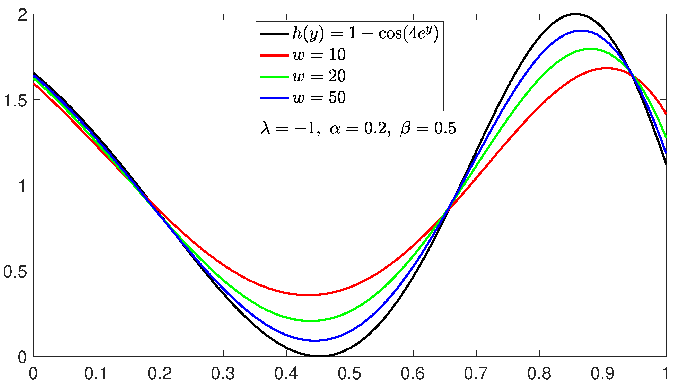
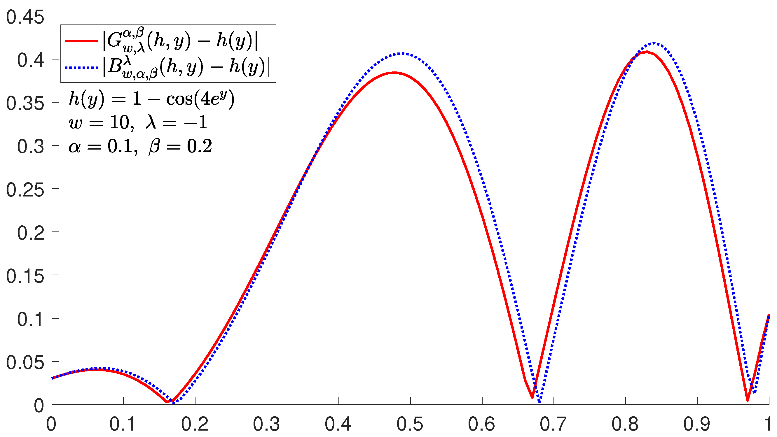
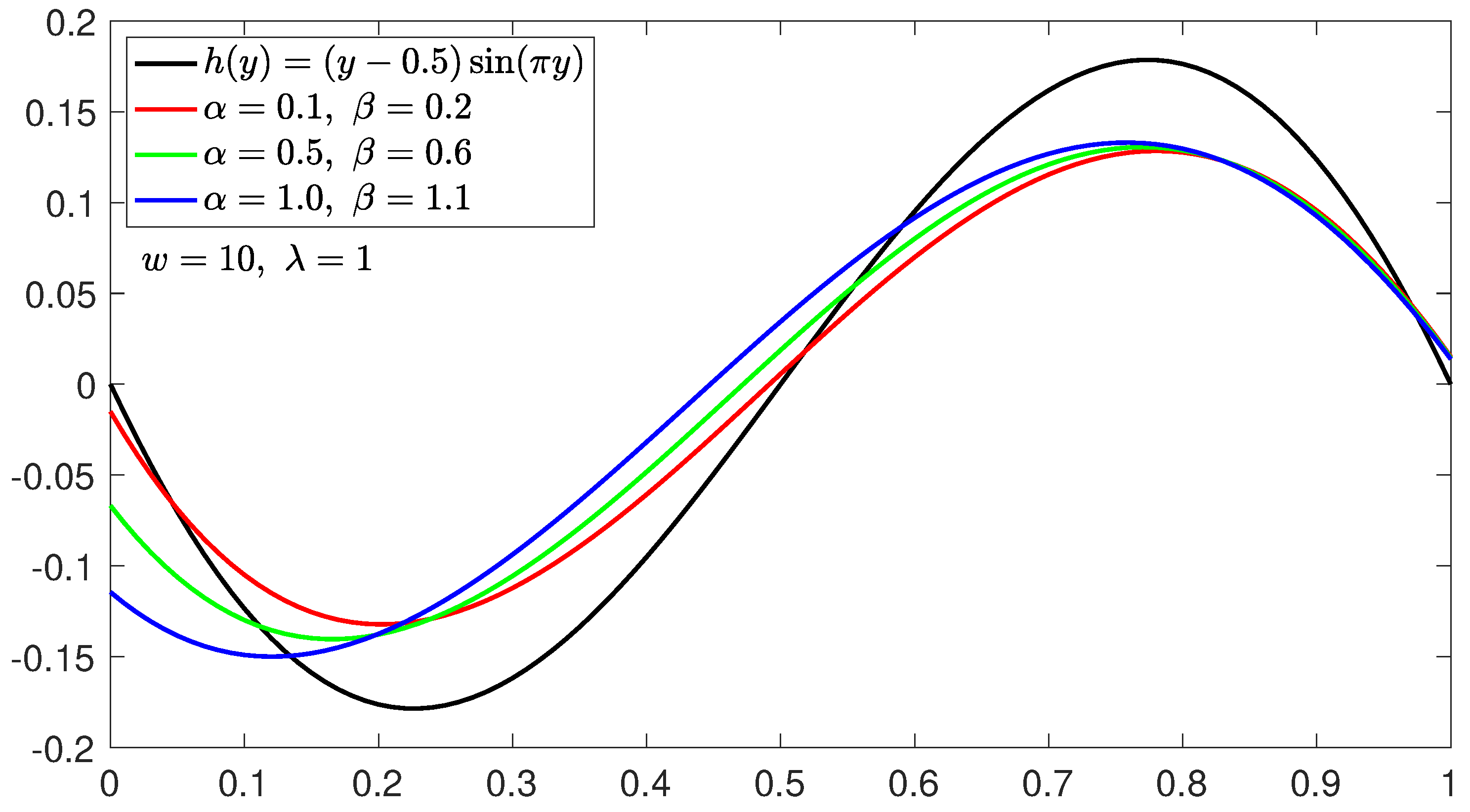
5. Some Numerical Examples and Graphs

In this section, we provide numerical examples to demonstrate the convergence properties of the newly defined operators $G_{\omega ,\lambda }^{\alpha ,\beta }\left(h\right)$. Additionally, we compare their convergence with the operators $B_{\omega ,\alpha ,\beta }^{\lambda }\left(h\right)$. To achieve this, we selected specific functions and analyzed their convergence behavior across different parameter settings.

Example 1.

We take the test function $h\left(y\right)=1-cos\left(4e^y\right)$. The graphs of $G_{\omega ,\lambda }^{\alpha ,\beta }(h;y)$ with $\lambda =-1,\alpha =0.2,\beta =0.5$ and different values of ω are shown in Figure 1. It can be seen from Figure 1 that with the increase in ω, $G_{\omega ,\lambda }^{\alpha ,\beta }\left(h\right)$ is getting closer and closer to function $h\left(y\right)$. In Figure 2, we fix $\omega =20$ and $\lambda =1$, operators $G_{\omega ,\lambda }^{\alpha ,\beta }\left(h\right)$ and $h\left(x\right)$ with different values of the parameters α and β are shown. Figure 3 shows the absolute error of $G_{10,-1}^{0.1,0.2}(h;y)$ and $B_{10,0.1,0.2}^{-1}(h;y)$ on $h\left(y\right)$.

Table 1. The absolute error bound of $G_{\omega ,\lambda }^{\alpha ,\beta }(h;y)$ to $h\left(y\right)$.

$\mathit{\lambda }$	$\parallel {\mathit{G}}_{\mathit{\omega },\mathit{\lambda }}^{\mathit{\alpha },\mathit{\beta }}{\left(\mathit{h}\right)-\mathit{h}\parallel }_{\mathit{\infty }}$
	$\mathbf{\omega }=\mathbf{100}$	$\mathbf{\omega }=\mathbf{200}$	$\mathbf{\omega }=\mathbf{300}$	$\mathbf{\omega }=\mathbf{500}$	$\mathbf{\omega }=\mathbf{1000}$
$-1$	0.055302823	0.028169281	0.018896155	0.011394022	0.005718237
$-0.5$	0.055214697	0.028144068	0.018884464	0.011389672	0.005717122
0	0.055126571	0.028118854	0.018872772	0.011385321	0.005716008
$0.5$	0.055038445	0.028093641	0.018861081	0.011380971	0.005714894
1	0.054950318	0.028068427	0.01884939	0.011376621	0.005713779

and

Table 2. The absolute error bound of $B_{\omega ,\alpha ,\beta }^{\lambda }(h;y)$ to $h\left(y\right)$.

$\mathit{\lambda }$	$\parallel {\mathit{B}}_{\mathit{\omega },\mathit{\alpha },\mathit{\beta }}^{\mathit{\lambda }}{\left(\mathit{h}\right)-\mathit{h}\parallel }_{\mathit{\infty }}$
	$\mathbf{\omega }=\mathbf{100}$	$\mathbf{\omega }=\mathbf{200}$	$\mathbf{\omega }=\mathbf{300}$	$\mathbf{\omega }=\mathbf{500}$	$\mathbf{\omega }=\mathbf{1000}$
$-1$	0.055029304	0.028087973	0.018858053	0.011379733	0.005714556
$-0.5$	0.055077937	0.028103414	0.018865413	0.011382527	0.005715282
0	0.055126571	0.028118854	0.018872772	0.011385321	0.005716008
$0.5$	0.055175204	0.028134295	0.018880132	0.011388116	0.005716734
1	0.055223838	0.028149736	0.018887492	0.01139091	0.00571746

show the absolute error bound of $G_{\omega ,\lambda }^{\alpha ,\beta }(h;y)$ and $B_{\omega ,\alpha ,\beta }^{\lambda }(h;y)$ on the function $h\left(y\right)$ when $\alpha =0.1$ and $\beta =0.2$. As can be seen from Table 1 and Table 2, for fixed α and β, the closer λ is to 1, the smaller absolute error bound between $G_{\omega ,\lambda }^{\alpha ,\beta }\left(h\right)$ and $h\left(y\right)$. Conversely, the closer λ is to $-1$, the smaller absolute error bound between $B_{\omega ,\alpha ,\beta }^{\lambda }\left(h\right)$ and $h\left(y\right)$. But from the form of the basis function construction, it is obvious that the basis function form of the newly defined operator will be simpler.

Example 2.

We take the test function $h\left(y\right)=(y-0.5)sin\left(\pi y\right)$. The graphs of $G_{\omega ,\lambda }^{\alpha ,\beta }(h;y)$ with $\omega =10,\lambda =1$ and different values of α and β are shown in Figure 4. Figure 5 shows the absolute error of $G_{10,-1}^{0.1,0.2}(h;y)$ and $B_{10,0.1,0.2}^{-1}(h;y)$ on $h\left(y\right)$.

References

1. Weierstrass, K. Über die analytische Darstellbarkeit sogenannter willkürlicher Functionen einer reellen Veränderlichen. Sitzungsberichte der Königlich Preußischen Akad. Der Wiss. Berl. 1885, 2, 364. [Google Scholar]
2. Bernšteın, S.N. Démonstration du théoreme de Weierstrass fondée sur le calcul des probabilities. Comm. Soc. Math. Kharkov 1912, 13, 1–2. [Google Scholar]
3. Stancu, D.D. Approximation of function by a new class of polynomial operators. Rev. Roum. Mathématiques Pures Appliquées. Rom. J. Pure Appl. Math. Ed. Acad. Române 1968, 13, 1173–1194. [Google Scholar]
4. Gadjiev, A.D.; Ghorbanalizadeh, A.M. Approximation properties of a new type Bernstein–Stancu polynomials of one and two variables. Appl. Math. Comput. 2010, 216, 890–901. [Google Scholar] [CrossRef]
5. Uster, R.; İbikli, E. On The Rate of Convergence of The Stancu Type Bernstein Operators For Functions of Bounded Variation. Math. Sci. Appl. -Notes 2015, 3, 126–136. [Google Scholar] [CrossRef]
6. Dong, L.X.; Yu, D.S. Pointwise approximation by a Durrmeyer variant of Bernstein-Stancu operators. J. Inequalities Appl. 2017, 2017, 1–13. [Google Scholar] [CrossRef] [PubMed]
7. Çetin, N. On complex modified Bernstein-Stancu operators. Math. Found. Comput. 2023, 6, 63–77. [Google Scholar] [CrossRef]
8. Cai, Q.B.; Lian, B.Y.; Zhou, G. Approximation properties of λ-Bernstein operators. J. Inequalities Appl. 2018, 2018, 1–11. [Google Scholar] [CrossRef] [PubMed]
9. Acu, A.M.; Manav, N.; Sofonea, D.F. Approximation properties of λ-Kantorovich operators. J. Inequalities Appl. 2018, 2018, 1–12. [Google Scholar] [CrossRef] [PubMed]
10. Srivastava, H.M.; Özger, F.; Mohiuddine, S.A. Construction of Stancu-type Bernstein operators based on Bézier bases with shape parameter λ. Symmetry 2019, 11, 316. [Google Scholar] [CrossRef]
11. Kumar, A. Approximation properties of generalized λ-Bernstein–Kantorovich type operators. Rend. Del Circ. Mat. Palermo Ser. 2021, 70, 505–520. [Google Scholar] [CrossRef]
12. Cai, Q.B.; Torun, G.; Dinlemez Kantar, Ü. Approximation Properties of Generalized λ-Bernstein–Stancu-Type Operators. J. Math. Hindawi 2021, 2021, 5590439. [Google Scholar] [CrossRef]
13. Bodur, M.; Manav, N.; Tasdelen, F. Approximation properties of λ-Bernstein-kantorovich-stancu operators. Math. Slovaca 2022, 72, 141–152. [Google Scholar] [CrossRef]
14. Cai, Q.B.; Khan, A.; Mansoori, M.S.; Iliyas, M.; Khan, K. Approximation by λ-Bernstein type operators on triangular domain. Filomat 2023, 37, 1941–1958. [Google Scholar] [CrossRef]
15. Zhou, G.; Chen, S.; Zhao, G. Approximation properties of a new kind of λ-Bernstein Operators. 2024; in press. [Google Scholar]
16. DeVore, R.A.; Lorentz, G.G. Constructive Approximation; Springer: Berlin/Heidelberg, Germany, 1993. [Google Scholar]
17. Korovkin, P.P. On convergence of linear positive operators in the space of continuous functions (Russian). Dokl. Akad. Nauk. Sssr (NS) 1953, 90, 961–964. [Google Scholar]
Figure 1. The convergence of G 10 , 1 0.2 , 0.5 ( h ; y ) , G 20 , 1 0.2 , 0.5 ( h ; y ) , G 50 , 1 0.2 , 0.5 ( h ; y ) to h ( y ) .
Symmetry 16 01276 g001
Figure 2. The convergence of G 20 , 1 0.1 , 0.2 ( h ; y ) , G 20 , 1 0.5 , 0.6 ( h ; y ) , G 20 , 1 1.0 , 1.1 ( h ; y ) to h ( y ) .
Symmetry 16 01276 g002
Figure 3. Comparison of errors for G 10 , 1 0.1 , 0.2 ( h ; y ) and B 10 , 0.1 , 0.2 1 ( h ; y ) to h ( y ) .
Symmetry 16 01276 g003
Figure 4. The convergence of G 10 , 1 0.1 , 0.2 ( h ; y ) , G 10 , 1 0.5 , 0.6 ( h ; y ) , G 10 , 1 1.0 , 1.1 ( h ; y ) to h ( y ) .
Symmetry 16 01276 g004
Figure 5. Comparison of errors for G 10 , 1 0.1 , 0.2 ( h ; y ) and B 10 , 0.1 , 0.2 1 ( h ; y ) to h ( y ) .
Symmetry 16 01276 g005