Upper Bounds of the Third Hankel Determinant for Bi-Univalent Functions in Crescent-Shaped Domains

Abstract

This paper investigates the third Hankel determinant, denoted $H_3\left(1\right)$, for functions within the subclass $\mathcal{R}{\mathcal{S}}_{\sum }^{\mathrm{*}}\left(\lambda \right)$ of bi-univalent functions associated with crescent-shaped regions ${\phi }_{⦅}\left(z\right)=z+\sqrt{1+z^2}$. The primary aim of this study is to establish upper bounds for $H_3\left(1\right)$. By analyzing functions within this specific geometric context, we derive precise constraints on the determinant, thereby enhancing our understanding of its behavior. Our results and examples provide valuable insights into the properties of bi-univalent functions in crescent-shaped domains and contribute to the broader theory of analytic functions.

1. Introduction

We indicate by $\mathcal{A}$ the class of analytic functions that have the formula

$$f\left(z\right)=z+\sum _{n=2}^{\mathrm{\infty }}{a}_n{z}^n$$

(1)

in the disk $\mathbb{U}=\left\{z\in \mathbb{C}:\left|z\right|<1\right\}$. Consider also that $\mathcal{S}$ denotes the subclass of all functions $\mathcal{A}$ that are also univalent in $\mathbb{U}$. It is well known that every function $f\in \mathcal{S}$ has an inverse $g≔f^{-1}$ satisfying $g\left(f\left(z\right)\right)=z$ and $f\left(g\left(w\right)\right)=w\left(z\in \mathbb{U},\left|w\right|<R\left(f\right):R\left(f\right)\ge {\displaystyle \frac{1}{4}}\right)$ and given by

$$g\left(w\right)=w-a_2{w}^2+\left(2a_2^2-a_3\right)w^3-\left(5a_2^3-5a_2{a}_3+a_4\right)w^4+\cdots .$$

(2)

Let $f$ be a function in $\mathcal{S}$, and its inverse $g$ can be extended as a function belonging to $\mathcal{S}$; then, $f$ is called bi-univalent in $\mathbb{U}$ and denoted by $\mathsf{\Sigma }$. Subclasses of $\mathsf{\Sigma }$ are namely bi-starlike (bi-convex) of order $\vartheta (0\le \vartheta <1)$ and have been established by Brannan and Taha [1]. These classes are non-sharp coefficient estimates $\left|a_2\right|$ and $\left|a_3\right|$ (see [1,2]). However, the $n^{\mathrm{t}\mathrm{h}}$ Taylor–Maclaurin coefficients $\left|a_n\right|\left(n\in \left\{3,4,\dots \right\}\right)$ remain an unresolved challenge (see [1,2,3,4,5]).

Srivastava et al.’s pioneering work [6] has notably revived the study of bi-univalent functions in recent years. For a concise historical overview and various intriguing examples of functions within the class $\mathsf{\Sigma }$, one should refer to this influential research. Several authors have introduced and studied various subclasses of $\mathsf{\Sigma }$ in works that followed [6], in which they established non-sharp bounds for the initial Taylor–Maclaurin coefficients. For further details, refer to [1,2,3,4,5,7,8,9,10,11,12]. We note that $\mathsf{\Sigma }\ne \varphi$ $\mathsf{\Sigma }⊊\mathcal{S}$, since $z/1-z$ belongs to it, whereas the Koebe function does not belong to it.

In the following, an analytic function $f$ is subordinate to another $g$ if there exists an analytic function $\omega :\mathbb{U}⟶\mathbb{U}$ with $\omega \left(0\right)=0$ satisfying $f\left(z\right)=h\left(\omega \left(z\right)\right)(z\in \mathbb{U})$ and written as $f\prec h$.

Ma and Minda [13] investigated the integration of different subclasses of starlike and convex functions. They explored situations where one of the functions, specifically $z{f}^{\prime }\left(z\right)/f\left(z\right)$ or $1+z{f}^{″}\left(z\right)/f^{\prime }\left(z\right)$, is subordinated to another analytic function $\phi$. For this purpose, they considered the analytic function $\phi :\mathbb{U}⟶\mathbb{C}$ satisfying the four below conditions:

(1)

${\phi }^{\prime }\left(0\right)>0$;

(2)

$\phi$ is univalent with $Re\left(\phi \right)>0$;

(3)

$\phi \left(\mathbb{U}\right)$ is starlike with respect to $1$;

(4)

$\phi \left(\mathbb{U}\right)$ is symmetric about a real axis.

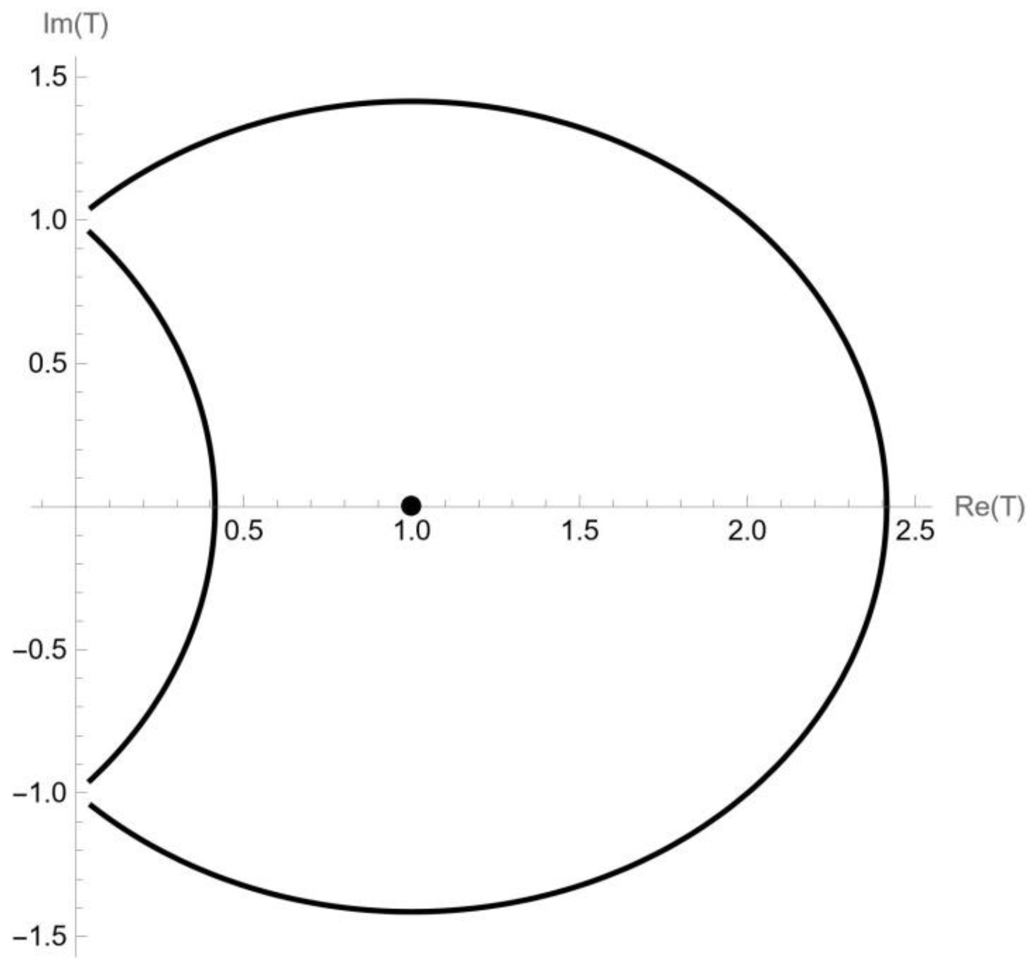
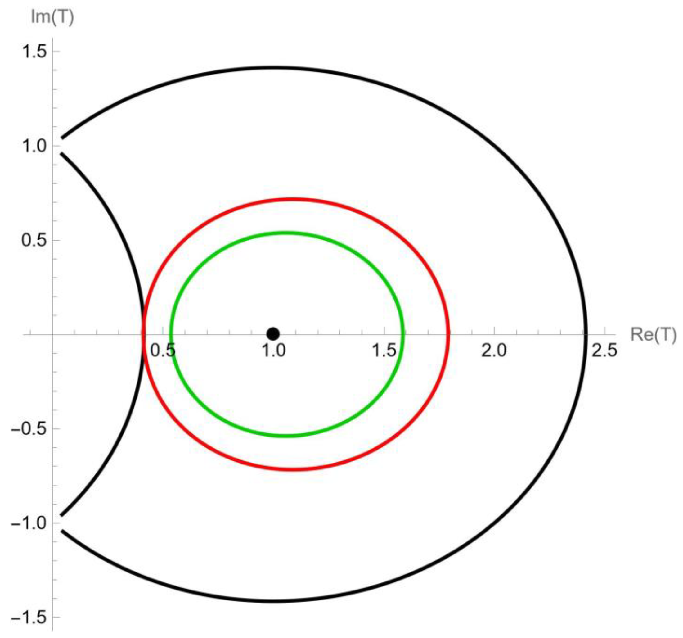
In addition, if $f$ and $g$ are Ma–Minda starlike (or Ma–Minda convex), then $f$ is called Ma–Minda bi-starlike (or Ma–Minda bi-convex), respectively.

Ravichandran and Kummar [14] studied the class of starlike functions of reciprocal order $\alpha (0\le \alpha <1)$ denoted by $\mathcal{R}{\mathcal{S}}^{\mathrm{*}}\left(\alpha \right)$ $\left(\mathcal{R}{\mathcal{S}}^{\mathrm{*}}≔\mathcal{R}{\mathcal{S}}^{\mathrm{*}}\left(0\right)\right)$ and characterized by the condition

$$Re\left({\displaystyle \frac{f\left(z\right)}{z{f}^{\prime }\left(z\right)}}\right)>\alpha .$$

In this paper, we introduce the bi-univalent Ma–Minda type $\mathcal{R}{\mathcal{S}}^{\mathrm{*}}$ denoted by $\mathcal{R}{\mathcal{S}}_{\sum }^{\mathrm{*}}\left(\lambda \right)$ (see Definition 2). However, we assume that $\phi$ satisfies conditions (1)–(4) above. The function

$${\phi }_{⦅}\left(z\right)=z+\sqrt{1+z^2}$$

(3)

maps $\mathbb{U}$ onto the crescent-shaped region given by $\{T\in \mathbb{C}:\left|T^2-1\right|<2\left|T\right|\}$, which satisfy the above four conditions (see Figure 1).

Definition 1

(see Raina and Sokól [15]; see also [16,17,18]). Let ${\mathcal{S}}_{⦅}^{*}$ be the class of all $f\in \mathcal{A}$ satisfying the subordination condition

$${\displaystyle \frac{z{f}^{\prime }\left(z\right)}{f\left(z\right)}}\prec z+\sqrt{1+z^2}.$$

Lemma 1 

(see [16]). For $\sqrt{2}-1<\epsilon \le \sqrt{2}+1$, let ${\xi }_{\epsilon }=1-\left|\sqrt{2}-\epsilon \right|$ and ${\Xi }_{\epsilon }=\sqrt{{\epsilon }^2+1}$. Then,

$$\left\{T\in \mathbb{C}:\left|T-\epsilon \right|<{\xi }_{\epsilon }\right\}\subseteq \left\{T\in \mathbb{C}:\left|T^2-1\right|<2\left|T\right|\right\}\subseteq \left\{T\in \mathbb{C}:\left|T-\epsilon \right|<{\Xi }_{\epsilon }\right\}.$$

Noonan and Thomas [19] defined the $qth$ Hankel determinant of any function $f$ with the expression

$$f\left(z\right)=\sum _{n=1}^{\mathrm{\infty }}{a}_n{z}^n\left(z\in \mathbb{U}\right),$$

by

$$H_q\left(n\right)=\left|\begin{array}{l}{a}_n{a}_{n+1}\cdots a_{n+q-1}\\ a_{n+1}{a}_{n+2}\cdots a_{n+q}\\ ⋮⋮⋮\\ a_{n+q-1}{a}_{n+q}\cdots a_{n+2q-2}\end{array}\right|\left(q\ge 1\right).$$

In particular, we have

$$H_3\left(1\right)=\left|\begin{array}{lll}{a}_1& a_2& a_3\\ a_2& a_3& a_4\\ a_3& a_4& a_5\end{array}\right|,\left(a_1=1\right).$$

By applying the triangle inequality for $H_3\left(1\right)$, we have

$$\left|H_3\left(1\right)\right|\le \left|a_3\right|\left|a_2{a}_4-a_3^2\right|-\left|a_4\right|\left|a_4-a_2{a}_3\right|+\left|a_5\right|\left|a_3-a_2^2\right|.$$

(4)

Fekete and Szegö [20] considered the well-known functional $H_2\left(1\right)$ (see also [21,22]). They performed an early study on the estimates of $\left|a_3-\beta a_2^2\right|$, with $\beta \in \mathbb{R}$; if $f\in \mathcal{A}$, then

$$\left|a_3-\beta a_2^2\right|=\left\{\begin{array}{l}4\beta -3,\beta \ge 1\\ 1+2{\mathrm{e}}^{\left(-{\displaystyle \frac{2\beta }{1-\beta }}\right)},0\le \beta \le 1\\ 3-4\beta ,\beta \le 0\end{array}\right.$$

Inspired by the investigation of the second Hankel determinant for various subclasses of $\mathsf{\Sigma }$ [23,24,25,26,27,28,29,30] and the third Hankel determinant for various subclasses of univalent functions [31,32,33,34,35], this article establishes the upper bound of $H_3\left(1\right)$ for functions within $\mathcal{R}{\mathcal{S}}_{\sum }^{\mathrm{*}}\left(\lambda \right)$.

Motivation. 

Bi-univalent functions associated with crescent-shaped domains represent an intriguing area of complex analysis and hold significant implications across various applied fields. Understanding the properties of these functions contributes to the development of more accurate mathematical models. By deriving upper bounds for the third Hankel determinant, this research provides deeper insights into the behavior of analytic functions in these domains. Furthermore, the results pave the way for future studies and applications, enhancing both mathematical understanding and practical model development.

Objectives. 

This study aims to analyze the third Hankel determinant for bi-univalent functions associated with crescent-shaped regions of these functions, while the second objective focuses on applying the results in specific fields. These objectives are essential in understanding the potential implications of these functions in some applications.

2. About $\mathcal{R}{\mathcal{S}}_{\sum }^{\mathbf{*}}\left(\mathsf{\lambda }\right)$

In this section, we will establish a subclass of $\mathsf{\Sigma }$ associated with crescent-shaped regions. Additionally, we present non-trivial examples and illustrate them geometrically using the Mathematica^TM program (version 13.2).

Definition 2.

Let $0\le \lambda \le 1$. A function $f\in \sum$, given by (1), is said to be in the class $\mathcal{R}{\mathcal{S}}_{\sum }^{*}\left(\lambda \right)$, if it satisfies the following subordinations:

$${\displaystyle \frac{\lambda z{f}^{\prime }\left(z\right)+(1-\lambda )f\left(z\right)}{\lambda z^2{f}^{″}\left(z\right)+z{f}^{\prime }\left(z\right)}}\prec {\phi }_{⦅}\left(z\right),$$

(5)

and

$${\displaystyle \frac{\lambda w{g}^{\prime }\left(w\right)+(1-\lambda )g\left(w\right)}{\lambda z^2{g}^{″}\left(w\right)+w{g}^{\prime }\left(w\right)}}\prec {\phi }_{⦅}\left(w\right),$$

(6)

where $z,w\in \mathbb{U}$ and $g:=f^{-1}$.

The below example gives the subclasses of $\mathcal{R}{\mathcal{S}}^{\mathrm{*}}$.

Example 1. 

The class $\mathcal{R}{\mathcal{S}}_{\sum }^{*}≔\mathcal{R}{\mathcal{S}}_{\sum }^{*}\left(0\right)$ is given by

$${\displaystyle \frac{f\left(z\right)}{z{f}^{\prime }\left(z\right)}}\prec {\phi }_{⦅}\left(z\right),$$

and

$${\displaystyle \frac{g\left(w\right)}{w{g}^{\prime }\left(w\right)}}\prec {\phi }_{⦅}\left(w\right).$$

The following example presents non-trivial functions that belong to the class of functions $\mathcal{R}{\mathcal{S}}_{\sum }^{*}\left(\lambda \right)$.

Example 2.

Consider the function

$$f_{\rho }\left(z\right)={\displaystyle \frac{z}{1+\rho z}}\left(\left|\rho \right|\le 1\right),$$

then

$$g_{\rho }\left(w\right)≔f_{\rho }^{-1}(w)={\displaystyle \frac{w}{1-\rho w}}$$

Clearly, $f_{\rho }$ and $g_{\rho }$ belong to $\mathcal{S}$ for $\left|\rho \right|\le 1$. By simple calculation, we have

$$F_{\lambda ,\rho }\left(z\right)≔{\displaystyle \frac{\lambda z{f}_{\rho }^{\prime }\left(z\right)+(1-\lambda )f_{\rho }\left(z\right)}{\lambda z^2{f}_{\rho }^{″}\left(z\right)+z{f}_{\rho }^{\prime }\left(z\right)}}={\displaystyle \frac{z+\rho \left(2-\lambda \right)z^2+{\rho }^2(1-\lambda )z^3}{z+\rho (1-2\lambda )z^2}}.$$

(7)

Similarly,

$$G_{\lambda ,\rho }\left(w\right)≔{\displaystyle \frac{\lambda w{g}_{\rho }^{\prime }\left(w\right)+(1-\lambda )g_{\rho }\left(w\right)}{\lambda w^2{g}_{\rho }^{″}\left(w\right)+w{g}_{\rho }^{\prime }\left(w\right)}}={\displaystyle \frac{w-\rho \left(2-\lambda \right)w^2+{\rho }^2(1-\lambda )w^3}{w-\rho (1-2\lambda )w^2}}.$$

(8)

In particular cases,

(1)

If $\lambda =0$, then (7) and (8) are reduced as follows:

$$F_{\rho }\left(z\right)≔F_{0,\rho }\left(z\right)=1+\rho z,\mathrm{a}\mathrm{n}\mathrm{d}{G}_{\rho }\left(w\right)≔G_{0,\rho }\left(z\right)=1-\rho w.$$

Since $\left|T-1\right|=\left|F_{\rho }\left(z\right)-1\right|=\left|\rho z\right|$, then $\left|z\right|⟶1$ leads to $\left|T-1\right|⟶\left|\rho \right|$. Lemma 1 gives

$$F_{\rho }\left(z\right)\prec {\phi }_{⦅}\left(z\right)⟺\left|\rho \right|\le 1-\left(\sqrt{2}-1\right)=2-\sqrt{2}.$$

Since $F_{\rho }\left(\mathbb{U}\right)=G_{\rho }\left(\mathbb{U}\right)$, then

$$G_{\rho }\left(w\right)\prec {\phi }_{⦅}\left(w\right)⟺\left|\rho \right|\le 2-\sqrt{2}.$$

Hence, $f_{\rho }\in \mathcal{R}{\mathcal{S}}_{\sum }^{*}$ if and only if $\left|\rho \right|\le 2-\sqrt{2}$ (see Figure 2).

(2)

If $\lambda =1/2$, then (7) and (8) are reduced as follows:

$$F_{{\displaystyle \frac{1}{2}},\rho }\left(z\right)=1+{\displaystyle \frac{3}{2}}\rho z+{\displaystyle \frac{1}{2}}{\rho }^2{z}^2,\mathrm{a}\mathrm{n}\mathrm{d}{G}_{{\displaystyle \frac{1}{2}},\rho }\left(w\right)=1-{\displaystyle \frac{3}{2}}\rho w+{\displaystyle \frac{1}{2}}{\rho }^2{w}^2.$$

Since $\left|T-1\right|=\left|F_{{\displaystyle \frac{1}{2}},\rho }\left(z\right)-1\right|=\left|{\displaystyle \frac{3}{2}}\rho z+{\displaystyle \frac{1}{2}}{\rho }^2{z}^2\right|$, then $\left|z\right|⟶1$ leads to $\left|T-1\right|⟶\left|{\displaystyle \frac{3}{2}}\rho +{\displaystyle \frac{1}{2}}{\rho }^2\right|$. Lemma 1 gives

$$F_{{\displaystyle \frac{1}{2}},\rho }\left(z\right)\prec {\phi }_{⦅}\left(z\right)⟺\left|{\displaystyle \frac{3}{2}}\rho +{\displaystyle \frac{1}{2}}{\rho }^2\right|\le 2-\sqrt{2}⟺-0.462\le \rho \le 0.3505.$$

$F_{\rho }\left(\mathbb{U}\right)=G_{\rho }\left(\mathbb{U}\right)$ leads to

$$G_{{\displaystyle \frac{1}{2}},\rho }\left(w\right)\prec {\phi }_{⦅}\left(w\right)⟺-0.462\le \rho \le 0.3505.$$

Hence, $f_{\rho }\in \mathcal{R}{\mathcal{S}}_{\mathsf{\Sigma }}^{*}\left(1/2\right)$ if and only if $-0.462\le \rho \le 0.3505$ (see Figure 3).

3. Hankel Estimates of $\mathcal{R}{\mathcal{S}}_{\sum }^{\mathit{*}}\left(\mathit{\lambda }\right)$

The subsequent lemmas are important in establishing our results.

Lemma 2 

(see [36]). Let $\mathcal{P}$ be the class of all analytic functions $p\left(z\right)$ of the form

$$p\left(z\right)=1+\sum _{n=1}^{\infty }{p}_n{z}^n,$$

(9)

with $Re\left(p\left(z\right)\right)>0$ for all $z\in \mathbb{U}$. Then, $\left|p_n\right|\le 2$, for every $n=1,2,\cdots$.

Lemma 3 

(see [37]). If the function $p\in \mathcal{P}$ is given by (9), then

$$2p_2=p_1^2+\left(4-p_1^2\right)x$$

$$4p_3=p_1^3+2p_1\left(4-p_1^2\right)x-p_1\left(4-p_1^2\right)x^2+2\left(4-p_1^2\right)\left(1-{\left|x\right|}^2\right)y,$$

for some $x,y$ with $\left|x\right|\le 1$ and $\left|y\right|\le 1$.

Theorem 1. 

Let $f\left(z\right)$ given by (1) be in the class $\mathcal{R}{\mathcal{S}}_{\sum }^{*}\left(\lambda \right)$, $0\le \lambda \le 1$. Then, we have

$$\left|a_2{a}_4-a_3^2\right|\le {\displaystyle \frac{8+77\lambda +46{\lambda }^2+16{\lambda }^3}{6{\left(1+\lambda \right)}^4(1+3\lambda )}}.$$

(10)

Proof. 

Let $f\in \mathcal{R}{\mathcal{S}}_{\sum }^{\mathrm{*}}\left(\lambda \right)$. Then, there exists $u,v:\mathbb{U}\to \mathbb{U}$ with $u\left(0\right)=v\left(0\right)=0,\left|u\left(z\right)\right|<1,\left|v\left(w\right)\right|<1,$ where

$${\displaystyle \frac{\lambda z{f}^{\prime }\left(z\right)+(1-\lambda )f\left(z\right)}{\lambda z^2{f}^{″}\left(z\right)+z{f}^{\prime }\left(z\right)}}={\phi }_{⦅}\left(u\left(z\right)\right),$$

(11)

and

$${\displaystyle \frac{\lambda w{g}^{\prime }\left(w\right)+(1-\lambda )g\left(w\right)}{\lambda z^2{g}^{″}\left(w\right)+w{g}^{\prime }\left(w\right)}}\prec {\phi }_{⦅}\left(v\left(w\right)\right).$$

(12)

Consider the functions $p,q\in \mathcal{P}$ with expansions

$$p\left(z\right)={\displaystyle \frac{1+u\left(z\right)}{1-u\left(z\right)}}=1+\sum _{n=1}^{\infty }{p}_n{z}^n,$$

and

$$q\left(z\right)={\displaystyle \frac{1+v\left(w\right)}{1-v\left(w\right)}}=1+\sum _{n=1}^{\infty }{q}_n{w}^n.$$

It follows that

$$u\left(z\right)={\displaystyle \frac{p\left(z\right)-1}{p\left(z\right)+1}}={\displaystyle \frac{1}{2}}\left[p_{1}z+\left(p_2-{\displaystyle \frac{p_1^2}{2}}\right)z^2+\left(p_3-p_1{p}_2+{\displaystyle \frac{p_1^3}{4}}\right)z^3+\dots \right],$$

(13)

and

$$v\left(w\right)={\displaystyle \frac{q\left(w\right)-1}{q\left(w\right)+1}}={\displaystyle \frac{1}{2}}\left[q_{1}w+\left(q_2-{\displaystyle \frac{q_1^2}{2}}\right)w^2+\left(q_3-q_1{q}_2+{\displaystyle \frac{q_1^3}{4}}\right)w^3+\dots \right].$$

(14)

Substituting (13) and (14) into (3), we obtain

$${\phi }_{⦅}\left(u\left(z\right)\right)=1+{\displaystyle \frac{p_1}{2}}z+\left({\displaystyle \frac{p_2}{2}}-{\displaystyle \frac{p_1^2}{8}}\right)z^2+\left({\displaystyle \frac{p_3}{2}}-{\displaystyle \frac{p_1{p}_2}{2}}+{\displaystyle \frac{p_1^3}{8}}\right)z^3+\dots ,$$

(15)

and

$${\phi }_{⦅}\left(v\left(w\right)\right)=1+{\displaystyle \frac{q_1}{2}}w+\left({\displaystyle \frac{q_2}{2}}-{\displaystyle \frac{q_1^2}{8}}\right)w^2+\left({\displaystyle \frac{q_3}{2}}-{\displaystyle \frac{q_1{q}_2}{2}}+{\displaystyle \frac{q_1^3}{8}}\right)w^3+\dots .$$

(16)

Since $f\in \mathsf{\Sigma }$ has the Maclurian series defined by (1), computation shows that its inverse $g:=f^{-1}$ has the expansion by (2), and we have

$$\begin{array}{l}{\displaystyle \frac{\lambda z{f}^{\prime }\left(z\right)+(1-\lambda )f\left(z\right)}{\lambda z^2{f}^{″}\left(z\right)+z{f}^{\prime }\left(z\right)}}=1-(1+\lambda )a_{2}z+2\left[{\left(1+\lambda \right)}^2{a}_2^2-\left(1+2\lambda \right)a_3\right]z^2\\ +\left[7\left(1+3\lambda +2{\lambda }^2\right)a_2{a}_3-4\left(1+3\lambda +3{\lambda }^2+{\lambda }^{3401.2)}\right)a_2^3-3\left(1+3\lambda \right)a_4\right]z^3\\ +2[5\left(1+4\lambda +3{\lambda }^2\right)a_2{a}_4-10\left(1+4\lambda +5{\lambda }^2+2{\lambda }^3\right)a_3{a}_2^2+3\left(1+4\lambda +4{\lambda }^2\right)a_3^2\\ +4\left(1+4\lambda +6{\lambda }^2+4{\lambda }^{3401.2)}+{\lambda }^{4401.2)}\right)a_2^4-2\left(1+4\lambda \right)a_5]z^4+\cdots ,\end{array}$$

(17)

and

$$\begin{gathered} \begin{array}{l}{\displaystyle \frac{\lambda w{g}^{\prime }\left(w\right)+(1-\lambda )g\left(w\right)}{\lambda z^2{g}^{″}\left(w\right)+w{g}^{\prime }\left(w\right)}}=1+(1+\lambda )a_{2}w+2\left[\left(1+2\lambda \right)a_3-\left(1+2\lambda -{\lambda }^2\right)a_2^2\right]w^2\\ +\left[\left(5+15\lambda +10{\lambda }^2+4{\lambda }^{3401.2)}\right)a_2^3-\left(8+24\lambda +{\lambda }^2\right)a_2{a}_3+3\left(1+3\lambda \right)a_4\right]w^3\\ +2[42\left(1+4\lambda \right)a_2{a}_3-3{\left(1+4\lambda -4{\lambda }^2\right)a}_3^2-\left(7+28\lambda -15{\lambda }^2\right)a_2{a}_4-\\ \left(5+28\lambda -47{\lambda }^2+24{\lambda }^{3401.2)}-4{\lambda }^{4401.2)}\right)a_2^4-\left(27+64\lambda +73{\lambda }^2-20{\lambda }^{3401.2)}\right)a_3{a}_2^2 \\ +2\left(1+4\lambda \right)a_5]w^4+\cdots .\end{array} \end{gathered}$$

(18)

From (15) and (17), we obtain that

$$-(1+\lambda )a_2={\displaystyle \frac{p_1}{2}},$$

(19)

$$2\left[{\left(1+\lambda \right)}^2{a}_2^2-\left(1+2\lambda \right)a_3\right]={\displaystyle \frac{p_2}{2}}-{\displaystyle \frac{p_1^2}{8}},$$

(20)

$$7\left(1+3\lambda +2{\lambda }^2\right)a_2{a}_3-4\left(1+3\lambda +3{\lambda }^2+{\lambda }^{3401.2)}\right)a_2^3-3\left(1+3\lambda \right)a_4={\displaystyle \frac{p_3}{2}}-{\displaystyle \frac{p_1{p}_2}{2}}+{\displaystyle \frac{p_1^3}{8}},$$

(21)

and

$$\begin{gathered} 2[5\left(1+4\lambda +3{\lambda }^2\right)a_2{a}_4-10\left(1+4\lambda +5{\lambda }^2+2{\lambda }^3\right)a_3{a}_2^2+3\left(1+4\lambda +4{\lambda }^2\right)a_3^2 \\ +4\left(1+4\lambda +6{\lambda }^2+4{\lambda }^{3401.2)}+{\lambda }^{4401.2)}\right)a_2^4-2\left(1+4\lambda \right)a_5] \\ ={\displaystyle \frac{p_1^2{p}_2}{4}}-{\displaystyle \frac{p_2^2}{8}}-{\displaystyle \frac{3p_1^4}{64}}-{\displaystyle \frac{p_1{p}_3}{2}}+{\displaystyle \frac{p_4}{2}}. \end{gathered}$$

(22)

Moreover, from (16) and (18), we obtain that

$$(1+\lambda )a_2={\displaystyle \frac{q_1}{2}},$$

(23)

$$2\left[\left(1+2\lambda \right)a_3-\left(1+2\lambda -{\lambda }^2\right)a_2^2\right]={\displaystyle \frac{q_2}{2}}-{\displaystyle \frac{q_1^2}{8}},$$

(24)

$$\left(5+15\lambda +10{\lambda }^2+4{\lambda }^{3401.2)}\right)a_2^3-\left(8+24\lambda +{\lambda }^2\right)a_2{a}_3+3\left(1+3\lambda \right)a_4={\displaystyle \frac{q_3}{2}}-{\displaystyle \frac{q_1{q}_2}{2}}+{\displaystyle \frac{q_1^3}{8}},$$

(25)

and

$$\begin{gathered} \begin{array}{l}2[42\left(1+4\lambda \right)a_2{a}_3-3{\left(1+4\lambda -4{\lambda }^2\right)a}_3^2-\left(7+28\lambda -15{\lambda }^2\right)a_2{a}_4-\\ \left(5+28\lambda -47{\lambda }^2+24{\lambda }^{3401.2)}-4{\lambda }^{4401.2)}\right)a_2^4-\left(27+64\lambda +73{\lambda }^2-20{\lambda }^{3401.2)}\right)a_3{a}_2^2 \\ +2\left(1+4\lambda \right)a_5]\\ ={\displaystyle \frac{q_1^2{q}_2}{4}}-{\displaystyle \frac{q_2^2}{8}}-{\displaystyle \frac{3q_1^4}{64}}-{\displaystyle \frac{q_1{q}_3}{2}}+{\displaystyle \frac{q_4}{2}}.\end{array} \end{gathered}$$

(26)

It follows from (19) and (23) that

$$a_2={\displaystyle \frac{-p_1}{2(1+\lambda )}}={\displaystyle \frac{q_1}{2(1+\lambda )}},$$

(27)

i.e.,

$$p_1=-q_1.$$

(28)

Subtracting (24) from (20) and considering (27), we obtain

$$a_3={\displaystyle \frac{p_1^2}{4{(1+\lambda )}^2}}-{\displaystyle \frac{p_2-q_2}{8\left(1+2\lambda \right)}}.$$

(29)

Moreover, subtracting (25) from (21) and considering (27) and (29), we find that

$$\begin{array}{l}{a}_4={\displaystyle \frac{5p_1\left(p_2-q_2\right)}{32\left(1+\lambda \right)\left(1+2\lambda \right)\left(1+3\lambda \right)}}+{\displaystyle \frac{\left(-6+27\lambda +22{\lambda }^2+8{\lambda }^3\right)p_1^3}{48{\left(1+\lambda \right)}^3\left(1+3\lambda \right)}}+{\displaystyle \frac{p_1\left(p_2+q_2\right)}{12\left(1+3\lambda \right)}}\\ -{\displaystyle \frac{\left(p_3-q_3\right)}{12\left(1+3\lambda \right)}}-{\displaystyle \frac{\left(p_1^3-q_1^3\right)}{48\left(1+3\lambda \right)}}.\end{array}$$

(30)

Hence, by (25), (27), and (28), it follows that

$$\begin{gathered} a_2{a}_4-a_3^2={\displaystyle \frac{-5p_1^2\left(p_2-q_2\right)}{64{\left(1+\lambda \right)}^2\left(1+2\lambda \right)\left(1+3\lambda \right)}}+{\displaystyle \frac{\left(-6+27\lambda +22{\lambda }^2+8{\lambda }^3\right)p_1^4}{96{\left(1+\lambda \right)}^4\left(1+3\lambda \right)}} \\ -{\displaystyle \frac{p_1^2\left(p_2+q_2\right)-p_1\left(p_3-q_3\right)}{24\left(1+\lambda \right)\left(1+3\lambda \right)}} \\ +{\displaystyle \frac{p_1^4}{48\left(1+\lambda \right)\left(1+3\lambda \right)}}-{\displaystyle \frac{p_1^4}{16{\left(1+\lambda \right)}^4}}+{\displaystyle \frac{p_1^2\left(p_2-q_2\right)}{16{\left(1+\lambda \right)}^2\left(1+2\lambda \right)}}-{\displaystyle \frac{{\left(p_2-q_2\right)}^2}{64{(1+2\lambda )}^2}}. \end{gathered}$$

(31)

According Lemma 3 and (28), we obtain

$$p_2-q_2={\displaystyle \frac{4-p_1^2}{2}}\left(x-y\right),p_2+q_2=p_1^2+{\displaystyle \frac{4-p_1^2}{2}}\left(x+y\right),$$

(32)

and

$$p_3-q_3={\displaystyle \frac{p_1^3}{2}}+{\displaystyle \frac{\left(4-p_1^2\right)p_1}{2}}\left(x+y\right)-{\displaystyle \frac{\left(4-p_1^2\right)p_1}{4}}\left(x^2+y^2\right)+{\displaystyle \frac{4-p_1^2}{2}}[(1-{\left|x\right|}^2)z-\left(1-{\left|y\right|}^2\right)w],$$

(33)

for some $x,y,z$ and $w$ with $\left|x\right|\le 1,\left|y\right|\le 1$ and $\left|w\right|\le 1$.

Since $p\in \mathcal{P}$, we have $\left|p_1\right|\le 2$. Letting $p_1=p$, we may assume without loss of generality that $p\in [0,2]$. Thus, substituting expressions (32) and (33) in (31), and letting $\gamma =\left|x\right|$ and $\delta =\left|y\right|$, we have

$$\left|a_2{a}_4-a_3^2\right|\le F_1+F_2\left(\gamma +\delta \right)+F_3\left({\gamma }^2+{\delta }^2\right)+F_4{\left(\gamma +\delta \right)}^2=:F\left(\gamma ,\delta \right),$$

where

$$F_1=F_1\left(\lambda ,p\right)={\displaystyle \frac{(8+77\lambda +46{\lambda }^2+16{\lambda }^3)p^4}{96{\left(1+\lambda \right)}^4(1+3\lambda )}}\ge 0,$$

$$F_2=F_2\left(\lambda ,p\right)={\displaystyle \frac{(13+84\lambda +32{\lambda }^2)\left(4-p^2\right)p^2}{384{\left(1+\lambda \right)}^2(1+2\lambda )(1+3\lambda )}}\ge 0,$$

$$F_3=F_3\left(\lambda ,p\right)={\displaystyle \frac{\left(4-p^2\right)p(P-2)}{96(1+\lambda )(1+3\lambda )}}\le 0,$$

and

$$F_4=F_4\left(\lambda ,p\right)={\displaystyle \frac{{(4-p^2)}^2}{256{\left(1+2\lambda \right)}^2}}\ge 0.$$

We wish to maximize $F\left(\gamma ,\delta \right)$ in the closed square $\left[0,1\right]\times [0,1]$ for $p\in [0,2]$, because $F_3+2F_2\ge 0$ and $F_3\le 0$, and we conclude that $p\in (0,2)$.

$F_{\gamma \gamma }{F}_{\delta \delta }-{\left(F_{\gamma \delta }\right)}^2<0$. Thus, the function $F$ cannot have a local maximum in the interior of the closed square. Now, we investigate the maximum of $F$ on the boundary of the closed square, such that $\gamma =0$ and $0\le \delta \le 1$, and we obtain

$$F\left(0,\delta \right)=\Phi \left(\delta \right)=F_1+F_2\delta +\left(F_3+F_4\right){\delta }^2.$$

Now, we deal with the two below cases.

• Case 1: Assume that $F_3+F_4\ge 0$. In this case, for $0\le \delta \le 1$, and any fixed $p$ with $0\le p<2$, it is clear that

  $${\Phi }^{\prime }\left(\delta \right)=F_2+2\left(F_3+F_4\right)\delta >0,$$

  i.e., $\Phi \left(\delta \right)$ is an increasing function. Hence, for fixed $p\in [0,2]$, the maximum of $\Phi \left(\delta \right)$ occurs at $\delta =1$ and

  $$\max \Phi \left(\delta \right)=\Phi \left(1\right)=F_1+F_2+F_3{+F}_4.$$
• Case 2: $F_3+F_4<0$, because $2\left(F_3+F_4\right)+F_2\ge 0$, $0<\delta <1$, where $0<p<2$, and it is evident that $2\left(F_3+F_4\right)+F_2<2\left(F_3+F_4\right)\delta +F_2<F_2$ and $\Phi \left(\delta \right)>0$. Thus, the maximum of $\Phi \left(\delta \right)$ occurs at $\gamma =1$ and $0\le \delta \le 1$, and we obtain

  $$F\left(1,\delta \right)=\theta \left(\delta \right)=\left(F_3+F_4\right){\delta }^2+\left(F_2+2F_4\right)\delta +F_1+F_2+F_3+F_4,$$

  so, from the cases of $F_3+F_4$, we obtain

  $$\max \theta \left(\delta \right)=\theta \left(1\right)=F_1+2F_2+2F_3+4F_4.$$

Since $\Phi \left(1\right)\le \theta \left(1\right)$, we obtain $\max \left(F\left(\gamma ,\delta \right)\right)=F(1,1)$ on the boundary of square $\left[0,1\right]\times [0,1]$. We define the real function $T$ on $(0,1)$ by

$$T\left(p\right)=\max \left(F\left(\gamma ,\delta \right)\right)=F\left(1,1\right)=F_1+2F_2+2F_3+4F_4.$$

Placing $F_1,F_2,F_3$ and $F_4$ in the function $T$, we obtain

$$T\left(p\right)=Q+R+S,$$

where

$$Q={\displaystyle \frac{(8+77\lambda +46{\lambda }^2+16{\lambda }^3)p^4}{96{\left(1+\lambda \right)}^4(1+3\lambda )}},$$

$$R={\displaystyle \frac{\left(4-p^2\right)p(P-2)}{48(1+\lambda )(1+3\lambda )}},$$

and

$$S={\displaystyle \frac{\left[\left(13+84\lambda +32{\lambda }^2\right)\left(1+2\lambda \right)+3{\left(1+\lambda \right)}^2(1+3\lambda )\right](4-p^2)p^2}{192{\left(1+\lambda \right)}^2{\left(1+2\lambda \right)}^2(1+3\lambda )}}.$$

After a few calculations, we conclude that $T\left(p\right)$ is an increasing function of $p$. Therefore, we obtain the maximum of $T\left(p\right)$ on $p=2$ and

$$\max T\left(p\right)=T\left(2\right)={\displaystyle \frac{8+77\lambda +46{\lambda }^2+16{\lambda }^3}{6{\left(1+\lambda \right)}^4(1+3\lambda )}}.$$

Consequently, this completes the proof. □

Theorem 2. 

Let $f\left(z\right)\in \mathcal{R}{\mathcal{S}}_{\sum }^{*}\left(\lambda \right),0\le \lambda \le 1$. Then, we have

$$\left|a_2{a}_3-a_4\right|\le \left\{\begin{array}{l}{\displaystyle \frac{8-3\lambda +2{\lambda }^2}{6{\left(1+\lambda \right)}^3(1+3\lambda )}},m\le p\le 2\\ {\displaystyle \frac{1}{3(1+3\lambda )}},0\le p\le m,\end{array}\right.$$

(34)

where

$$m={\displaystyle \frac{-d_3\pm \sqrt{d_3^2-12\left(d_1-d_2\right)d_2}}{3(m_1-m_2)}},$$

$$d_1={\displaystyle \frac{8-3\lambda +2{\lambda }^2}{48{\left(1+\lambda \right)}^3(1+3\lambda )}},$$

$$d_2={\displaystyle \frac{\left(7+66\lambda +32{\lambda }^2\right)+4\left(1+\lambda \right)\left(1+2\lambda \right)}{192\left(1+\lambda \right)\left(1+2\lambda \right)(1+3\lambda )}},$$

and

$$d_3={\displaystyle \frac{1}{12\left(1+3\lambda \right)}}.$$

Proof. 

From (27), (29), and (30), we obtain

$$\left|a_2{a}_3-a_4\right|=\left|{\displaystyle \frac{\left(2-21\lambda -16{\lambda }^2-6{\lambda }^3\right)p_1^3}{48{\left(1+\lambda \right)}^3(1+3\lambda )}}+{\displaystyle \frac{\left(6\lambda -3\right)p_1\left(p_2-q_2\right)}{32\left(1+\lambda \right)\left(1+2\lambda \right)\left(1+3\lambda \right)}}-{\displaystyle \frac{p_1\left(p_2+q_2\right)}{12\left(1+3\lambda \right)}}+{\displaystyle \frac{\left(p_3-q_3\right)}{12\left(1+3\lambda \right)}}\right|.$$

According to Lemma 3, we suppose, without any restriction, that $p\in [0,2]$, such that $p_1=p$. Therefore, for ${\eta }_1=\left|x\right|$ and ${\eta }_2=\left|y\right|$, we have

$$\left|a_2{a}_3-a_4\right|\le G_1+G_2\left({\eta }_1+{\eta }_2\right)+G_3\left({\eta }_1^2+{\eta }_2^2\right)=G\left({\eta }_1,{\eta }_2\right),$$

where

$$G_1(\lambda ,p)={\displaystyle \frac{(8-3\lambda +2{\lambda }^2)p^3}{48{\left(1+\lambda \right)}^3(1+3\lambda )}}\ge 0,$$

$$G_2(\lambda ,p)={\displaystyle \frac{\left(7+66\lambda +32{\lambda }^2\right)\left(4-p^2\right)p}{192\left(1+\lambda \right)\left(1+2\lambda \right)\left(1+3\lambda \right)}}\ge 0,$$

and

$$G_3\left(\lambda ,p\right)={\displaystyle \frac{\left(4-p^2\right)(p-2)}{48(1+3\lambda )}}\le 0.$$

We use the same proof technique as in Theorem 1. Thus, the maximum occurs at ${\eta }_1=1$ and ${\eta }_2=1$ in closed square $[0,2]$,

$$\theta \left(p\right)=\max \left(G\left({\eta }_1,{\eta }_2\right)\right)=G_1+2\left(G_2+G_3\right).$$

Substituting the values of $G_1,G_2$ and $G_3$ in $\theta \left(p\right)$, we obtain

$$\theta \left(p\right)=d_1{p}^3+d_{2}p\left(4-p^2\right)+d_3\left(4-p^2\right),$$

where

$$d_1={\displaystyle \frac{8-3\lambda +2{\lambda }^2}{48{\left(1+\lambda \right)}^3(1+3\lambda )}},$$

$$d_2={\displaystyle \frac{\left(7+66\lambda +32{\lambda }^2\right)+4\left(1+\lambda \right)\left(1+2\lambda \right)}{192\left(1+\lambda \right)\left(1+2\lambda \right)(1+3\lambda )}},\mathrm{a}\mathrm{n}\mathrm{d}$$

$$d_3={\displaystyle \frac{1}{12\left(1+3\lambda \right)}}.$$

Therefore,

$$\begin{gathered} {\theta }^{\prime }\left(p\right)=3\left(d_1-d_2\right)p^2+2d_{3}p+4d_2, \\ {\theta }^{″}\left(p\right)=6\left(d_1-d_2\right)p+2d_3, \end{gathered}$$

if $d_1-d_2>0$, then $d_1>d_2$. Hence, ${\theta }^{\prime }\left(p\right)>0$, and so $\theta \left(p\right)$ is an increasing function on the closed interval $[0,2]$. Therefore, the function $\theta \left(p\right)$ gives the maximum value at $p=2$, i.e.,

$$\left|a_2{a}_3-a_4\right|\le \theta \left(2\right)={\displaystyle \frac{8-3\lambda +2{\lambda }^2}{6{\left(1+\lambda \right)}^3\left(1+3\lambda \right)}}.$$

On the other hand, if $d_1-d_2<0$ with ${\theta }^{\prime }\left(p\right)=0$, we obtain the following result

$$p=m={\displaystyle \frac{-d_3\pm \sqrt{d_3^2-12\left(d_1-d_2\right)d_2}}{3(d_1-d_2)}},$$

whenever $m<p\le 2$. Then, we obtain ${\theta }^{\prime }\left(p\right)>0$, which means that this function is on the closed interval $[0,2]$. Thus, $\theta \left(p\right)$ has the maximum value at $p=2$, which means that $\theta \left(p\right)$ is a decreasing function on the closed interval $[0,2]$; thus, $\theta \left(p\right)$ gives the maximum value at $p=0$, i.e.,

$$\left|a_2{a}_3-a_4\right|\le \theta \left(0\right)={\displaystyle \frac{1}{3(1+3\lambda )}}.$$

Thus, the proof has been thoroughly established. □

Theorem 3. 

Let $f\left(z\right)\in \mathcal{R}{\mathcal{S}}_{\sum }^{*}\left(\lambda \right),0\le \lambda \le 1$. Then, we have

$$\left|a_3-a_2^2\right|\le {\displaystyle \frac{1}{2(1+2\lambda )}},$$

(35)

$$\left|a_3\right|\le {\displaystyle \frac{1}{{(1+\lambda )}^2}}+{\displaystyle \frac{1}{2(1+2\lambda )}}.$$

(36)

Proof. 

By using (29) and Lemma 2, we obtain (36).

The following Fekete–Szegö functional, for $\mu \in \mathbb{C}$ and $f\in \mathcal{R}{\mathcal{S}}_{\sum }^{*}\left(\lambda \right)$,

$$a_3-{\mu a}_2^2={\displaystyle \frac{p_1^2}{{4(1+\lambda )}^2}}\left(1-\mu \right)+{\displaystyle \frac{p_2-q_2}{8(1+2\lambda )}}.$$

By Lemma 2, we obtain

$$\left|a_3-{\mu a}_2^2\right|\le {\displaystyle \frac{\left(1-\mu \right)}{{(1+\lambda )}^2}}+{\displaystyle \frac{1}{2(1+2\lambda )}},$$

and, for $\mu =1,$ we obtain (35). □

Theorem 4. 

Let $f\left(z\right)\in \mathcal{R}{\mathcal{S}}_{\sum }^{*}\left(\lambda \right),0\le \lambda \le 1$. Then, we have

$$\left|a_4\right|\le {\displaystyle \frac{5}{4\left(1+\lambda \right)\left(1+2\lambda \right)\left(1+3\lambda \right)}}+{\displaystyle \frac{\left(-6+27\lambda +22{\lambda }^2+8{\lambda }^3\right)}{6{\left(1+\lambda \right)}^3\left(1+3\lambda \right)}}+{\displaystyle \frac{4}{3(1+3\lambda )}},$$

(37)

$$\begin{gathered} \left|a_5\right|\le {\displaystyle \frac{26+95\lambda +132{\lambda }^2-33{\lambda }^3+60{\lambda }^4}{4{\left(1+\lambda \right)}^4\left(1+3\lambda \right)\left(1+4\lambda \right)}}+{\displaystyle \frac{126+478\lambda +135{\lambda }^2}{32{\left(1+\lambda \right)}^2\left(1+2\lambda \right)\left(1+3\lambda \right)\left(1+4\lambda \right)}}+{\displaystyle \frac{72+276\lambda -81{\lambda }^2}{24\left(1+\lambda \right)\left(1+3\lambda \right)\left(1+4\lambda \right)}} \\ +{\displaystyle \frac{42\left(1+\lambda \right)\left(1+2\lambda \right)+21{\left(1+3\lambda \right)}^2}{4\left(1+\lambda \right)\left(1+2\lambda \right){\left(1+3\lambda \right)}^2}}+{\displaystyle \frac{1}{32{\left(1+2\lambda \right)}^2\left(1+4\lambda \right)}}+{\displaystyle \frac{9}{8\left(1+4\lambda \right)}}. \end{gathered}$$

(38)

Proof. 

From (30) and by Lemma 2, we obtain (37).

Subtracting (26) from (22), we have

$$\begin{gathered} 8\left(1+4\lambda \right)a_5=\left(24+92\lambda -27{\lambda }^2\right)a_2{a}_4+\left(34+48\lambda +46{\lambda }^2-80{\lambda }^3\right){a_{3}a}_2^2+{\left(12+48\lambda \right)a}_3^2 \\ +\left(18+88\lambda -46{\lambda }^2+80{\lambda }^3\right)a_2^4-84\left(1+4\lambda \right)a_2{a}_3-{\displaystyle \frac{p_1\left(p_2-q_2\right)}{4}}+{\displaystyle \frac{p_2^2-q_2^2}{8}}+{\displaystyle \frac{p_1\left(p_3+q_3\right)}{2}}+{\displaystyle \frac{\left(p_4-q_4\right)}{2}}. \end{gathered}$$

Substituting properly (27), (29), and (30), we have

$$\begin{array}{ll}8\left(1+4\lambda \right)a_5=& {\displaystyle \frac{\left(26+95\lambda +132{\lambda }^2-33{\lambda }^3+60{\lambda }^4\right)p_1^4}{8{\left(1+\lambda \right)}^4\left(1+3\lambda \right)}}+{\displaystyle \frac{21\left(1+4\lambda \right)p_1^3}{2{\left(1+\lambda \right)}^3}}\\ & -{\displaystyle \frac{\left(24+92\lambda -27{\lambda }^2\right)p_1^2\left(p_2+q_2\right)}{24\left(1+\lambda \right)\left(1+3\lambda \right)}}+{\displaystyle \frac{\left(24+92\lambda -27{\lambda }^2\right)p_1\left(p_3-q_3\right)}{24\left(1+\lambda \right)\left(1+3\lambda \right)}}\\ & +{\displaystyle \frac{{\left(p_2-q_2\right)}^2}{64{\left(1+2\lambda \right)}^2}}-{\displaystyle \frac{\left(126+478\lambda -135{\lambda }^2\right)p_1^2\left(p_2-q_2\right)}{64{\left(1+\lambda \right)}^2\left(1+2\lambda \right)\left(1+3\lambda \right)}}\\ & -{\displaystyle \frac{21\left(1+4\lambda \right)p_1\left(p_2-q_2\right)}{4\left(1+\lambda \right)\left(1+2\lambda \right)}}-{\displaystyle \frac{p_1\left(p_2-q_2\right)}{4}}+{\displaystyle \frac{p_2^2-q_2^2}{8}}+{\displaystyle \frac{p_1\left(p_3+q_3\right)}{2}}\\ & +{\displaystyle \frac{\left(p_4-q_4\right)}{2}}.\end{array}$$

By applying Lemma 2, we obtain (38). □

Theorem 5. 

Let $f\left(z\right)\in \mathcal{R}{\mathcal{S}}_{\sum }^{*}\left(\lambda \right),0\le \lambda \le 1.$ Then, we have

$$\left|H_3\left(1\right)\right|\le \left\{\begin{array}{l}B{\mathcal{B}}_1-{\mathcal{B}}_2\left[{\displaystyle \frac{8-3\lambda +2{\lambda }^2}{6{\left(1+\lambda \right)}^3(1+3\lambda )}}\right]+{\mathcal{B}}_3{\mathcal{B}}_4,m\le p\le 2\\ B{\mathcal{B}}_1-\left[{\displaystyle \frac{1}{3(1+3\lambda )}}\right]{\mathcal{B}}_2+{\mathcal{B}}_3{\mathcal{B}}_4,0\le p\le m,\end{array}\right.$$

(39)

where $\mathcal{B}{,\mathcal{B}}_1,{\mathcal{B}}_2,{\mathcal{B}}_3{,\mathcal{B}}_4$, and $m$ are given by (36), (10), (37), (38), and (35), respectively.

Proof. 

Since $H_3\left(1\right)=a_3\left(a_2{a}_4-a_3^2\right)-a_4\left(a_4-a_2{a}_3\right)+a_5\left(a_3-a_2^2\right),$ applying the triangle inequality, we have (4). Substituting (36), (10), (37), (38), and (35) into (4), we obtain (39). □

4. Conclusions

In this study, we have thoroughly examined the third Hankel determinant for functions belonging to a specific subclass of bi-univalent functions associated with the crescent-shaped region. Our investigation revealed that the upper bounds for this determinant can be precisely determined, contributing valuable insights into the behavior and properties of such functions within the given geometric context.

The analysis demonstrated that the upper bounds obtained are significant in understanding the functions’ characteristics in the crescent-shaped region, providing a clearer picture of the constraints and limitations imposed by this geometric domain. The results not only advance our knowledge of Hankel determinants in relation to bi-univalent functions but also offer potential pathways for further research in this area.

Future studies could explore the extension of these results to other geometric regions, higher-order Hankel determinants, or Toeplitz determinants or deal with fractional derivatives (see [38,39]), which may uncover additional relationships and applications in the theory of analytic functions. The findings presented here lay a robust foundation for such advancements and underscore the importance of geometric considerations in the study of function theory.

In conclusion, the insights gained from our analysis of the third Hankel determinant enhance our understanding of bi-univalent functions and their associated determinants in crescent-shaped regions, marking a significant contribution to the field of complex analysis.

References

1. Brannan, D.A.; Taha, T.S. On some classes of bi-univalent functions. Studia Univ. Babes-Bolyai Math. 1986, 31, 70–77. [Google Scholar]
2. Taha, T.S. Topics in Univalent Function Theory. Ph.D. Thesis, University of London, London, UK, 1981. [Google Scholar]
3. Brannan, D.A.; Clunie, J.G. Aspects of Contemporary Complex Analysis. In Proceedings of the NATO Advanced Study Institute held at the University of Durham, Durham, UK, 1–20 July 1979; Academic Press: New York, NY, USA; London, UK, 1980. [Google Scholar]
4. Lewin, M. On a coefficient problem for bi-univalent functions. Proc. Am. Math. Soc. 1967, 18, 63–68. [Google Scholar] [CrossRef]
5. Netanyahu, E. The minimal distance of the image boundary from the origin and the second coefficient of a univalent function in |z| < 1. Arch. Ration. Mech. Anal. 1969, 32, 100–112. [Google Scholar] [CrossRef]
6. Srivastava, H.M.; Mishra, A.K.; Gochhayat, P. Certain subclasses of analytic and bi-univalent functions. Appl. Math. Lett. 2010, 23, 1188–1192. [Google Scholar] [CrossRef]
7. Xu, Q.-H.; Gui, Y.-C.; Srivastava, H.M. Coefficient estimates for a certain subclass of analytic and bi-univalent functions. Appl. Math. Lett. 2012, 25, 990–994. [Google Scholar] [CrossRef]
8. Xu, Q.-H.; Xiao, H.-G.; Srivastava, H.M. A certain general subclass of analytic and bi-univalent functions and associated coefficient estimate problems. Appl. Math. Comput. 2012, 218, 11461–11465. [Google Scholar] [CrossRef]
9. Shakir, Q.A.; Atshan, W.G. On third Hankel determinant for certain subclass of bi-univalent functions. Symmetry 2024, 16, 239. [Google Scholar] [CrossRef]
10. Sakar, F.M.; Aydoğan, S.M. Inequalities of bi-starlike functions involving Sigmoid function and Bernoulli Lemniscate by subordination. Int. J. Open Problems Compt. Math. 2023, 16, 71–82. [Google Scholar]
11. Swamy, S.R.; Breaz, D.; Venugopal, K.; Kempegowda, M.P.; Cotîrla, L.-I.; Rapeanu, E. Initial Coefficient Bounds Analysis for Novel Subclasses of Bi-Univalent Functions Linked with Lucas-Balancing Polynomials. Mathematics 2024, 12, 1325. [Google Scholar] [CrossRef]
12. Srivastava, H.M.; El-Deeb, S.M.; Breaz, D.; Cotîrla, L.-I.; Salagean, G.S. Bi-Concave Functions Connected with the Combination of the Binomial Series and the Confluent Hypergeometric Function. Symmetry 2024, 16, 226. [Google Scholar] [CrossRef]
13. Ma, W.; Minda, D. A unified treatment of some special classes of functions. In Proceedings of the Conference on Complex Analysis, Tianjin, China, 19–23 June 1992; Conference Proceedings and Lecture Notes in Analysis. Li, Z., Ren, F., Yang, L., Zhang, S., Eds.; International Press: Cambridge, MA, USA, 1994; Volume I, pp. 157–169. [Google Scholar]
14. Ravichandran, V.; Kumar, S.S. Argument estimate for starlike functions of reciprocal order. Southeast Asian Bull. Math. 2011, 35, 837–843. [Google Scholar]
15. Raina, R.K.; Sokół, J. Some properties related to a certain class of starlike functions. C. R. Math. Acad. Sci. Paris 2015, 353, 973–978. [Google Scholar] [CrossRef]
16. Gandhi, S.; Ravichandran, V. Starlike functions associated with a lune. Asian Eur. J. Math. 2017, 10, 1750064. [Google Scholar] [CrossRef]
17. Raina, R.K.; Sharma, P.; Sokól, J. Certain classes of analytic functions related to the crescent-shaped regions. J. Contemp. Math. Anal. 2018, 53, 355–362. [Google Scholar] [CrossRef]
18. Sharma, P.; Raina, R.K.; Sokól, J. Certain Ma–Minda type classes of analytic functions associated with the crescent-shaped region. Anal. Math. Phys. 2019, 9, 1887–1903. [Google Scholar] [CrossRef]
19. Noonan, J.W.; Thomas, D.K. On the second Hankel determinant of areally mean p-valent functions. Trans. Am. Math. Soc. 1076, 223, 337–346. [Google Scholar] [CrossRef]
20. Fekete, M.; Szegö, G. Eine Bemerkung über ungerade schlichte Funktionen. J. Lond. Math. Soc. 1933, 8, 85–89. [Google Scholar] [CrossRef]
21. Koepf, W. On the Fekete-Szego problem for close-to-convex functions. Proc. Am. Math. Soc. 1987, 101, 89–95. [Google Scholar]
22. Koepf, W. On the Fekete-Szego problem for close-to-convex functions II. Arch. Math. 1987, 49, 420–433. [Google Scholar] [CrossRef]
23. Altınkaya, S.; Yalçin, S. Second hankel determinant for a general subclass of bi-univalent functions. TWMS J. Pure Appl. Math. 2016, 7, 98–104. [Google Scholar]
24. Cağlar, M.; Deniz, E.; Srivastava, H.M. Second Hankel determinant for certain subclasses of bi-univalent functions. Turk. J. Math. 2017, 41, 694–706. [Google Scholar] [CrossRef]
25. Deniz, E.; Cağlar, M.; Orhan, H. Second Hankel determinant for bi-starlike and bi-convex functions of order β. Appl. Math. Comput. 2015, 271, 301–307. [Google Scholar]
26. Motamednezhad, A.; Bulboaca, T.; Adegani, E.A.; Dibagar, N. Second Hankel determinant for a subclass of analytic bi-univalent functions defined by subordination. Turk. J. Math. 2018, 42, 2798–2808. [Google Scholar] [CrossRef]
27. Mustafa, N.; Murugusundaramoorthy, G.; Janani, T. Second Hankel determinant for a certain subclass of bi-univalent functions. Mediterr. J. Math. 2018, 15, 119. [Google Scholar] [CrossRef]
28. Srivastava, H.M.; Altınkaya, S.; Yalçin, S. Hankel determinant for a subclass of bi-univalent functions defined by using a symmetric q-derivative operator. Filomat 2018, 32, 503–516. [Google Scholar] [CrossRef]
29. Srivastava, H.M.; Murugusundaramoorthy, G.; Bulboaca, T. The second Hankel determinant for subclasses of Bi-univalent functions associated with a nephroid domain. Rev. Real Acad. Cienc. Exactas Físicas Naturales. Ser. A. Matemáticas 2022, 116, 145. [Google Scholar] [CrossRef]
30. Zaprawa, P. On the Fekete-Szego problem for classes of bi-univalent functions. Bull. Belg. Math. Soc.-Simon Stevin 2014, 21, 169–178. [Google Scholar] [CrossRef]
31. Altınkaya, S.; Yalçin, S. Third Hankel determinant for Bazilevic functions. Adv. Math. 2016, 5, 91–96. [Google Scholar]
32. Kowalczyk, B.; Lecko, A.; Sim, Y.J. The sharp bound for the Hankel determinant of the third kind for convex functions. Bull. Aust. Math. Soc. 2018, 97, 435–445. [Google Scholar] [CrossRef]
33. Shanmugam, G.; Stephen, B.A.; Babalola, K.O. Third Hankel determinant for alpha-starlike functions. Gulf J. Math. 2014, 2, 107–113. [Google Scholar] [CrossRef]
34. Shi, L.; Srivastava, H.M.; Arif, M.; Hussain, S.; Khan, H. An investigation of the third Hankel determinant problem for certain subfamilies of univalent functions involving the exponential function. Symmetry 2019, 11, 598. [Google Scholar] [CrossRef]
35. Zaprawa, P. Third Hankel determinants for subclasses of univalent functions. Mediterr. J. Math. 2017, 14, 19. [Google Scholar] [CrossRef]
36. Duren, P.L. Univalent Functions, In Grundlehren der Mathematischen Wissenschaften, Band 259; Springer: New York, NY, USA; Berlin/Heidelberg, Germany; Tokyo, Japan, 1983. [Google Scholar]
37. Grenander, U.; Szegö, G. Toeplitz Forms and Their Applications, California Monographs in Mathematical Sciences; University of California Press: Berkeley, CA, USA, 1958. [Google Scholar]
38. Tayyah, A.S.; Atshan, W.G. New Results on r,k,µ-Riemann–Liouville Fractional Operators in Complex Domain with Applications. Fractal Fract. 2024, 8, 165. [Google Scholar] [CrossRef]
39. Aldawish, I.; Ibrahim, R.W. Studies on a new K-symbol analytic functions generated by a modified K-symbol Riemann-Liouville fractional calculus. MethodsX 2023, 11, 102398. [Google Scholar] [CrossRef]
Figure 1. Plot the boundary of φ U .
Symmetry 16 01281 g001
Figure 2. Plot of the boundaries of φ U and F 2 2 U in the colors black and red, respectively.
Symmetry 16 01281 g002
Figure 3. Plot of the boundaries of φ U , F 0.46 U , and F 0.3505 U in the colors black, red, and green, respectively.
Symmetry 16 01281 g003
Disclaimer/Publisher’s Note: The statements, opinions and data contained in all publications are solely those of the individual author(s) and contributor(s) and not of MDPI and/or the editor(s). MDPI and/or the editor(s) disclaim responsibility for any injury to people or property resulting from any ideas, methods, instructions or products referred to in the content.