On a Symmetry-Based Structural Deterministic Fractal Fractional Order Mathematical Model to Investigate Conjunctivitis Adenovirus Disease

Abstract

In the last few years, the conjunctivitis adenovirus disease has been investigated by using the concept of mathematical models. Hence, researchers have presented some mathematical models of the mentioned disease by using classical and fractional order derivatives. A complementary method involves analyzing the system of fractal fractional order equations by considering the set of symmetries of its solutions. By characterizing structures that relate to the fundamental dynamics of biological systems, symmetries offer a potent notion for the creation of mechanistic models. This study investigates a novel mathematical model for conjunctivitis adenovirus disease. Conjunctivitis is an infection in the eye that is caused by adenovirus, also known as pink eye disease. Adenovirus is a common virus that affects the eye’s mucosa. Infectious conjunctivitis is most common eye disease on the planet, impacting individuals across all age groups and demographics. We have formulated a model to investigate the transmission of the aforesaid disease and the impact of vaccination on its dynamics. Also, using mathematical analysis, the percentage of a population which needs vaccination to prevent the spreading of the mentioned disease can be investigated. Fractal fractional derivatives have been widely used in the last few years to study different infectious disease models. Hence, being inspired by the importance of fractal fractional theory to investigate the mentioned human eye-related disease, we derived some adequate results for the above model, including equilibrium points, reproductive number, and sensitivity analysis. Furthermore, by utilizing fixed point theory and numerical techniques, adequate requirements were established for the existence theory, Ulam–Hyers stability, and approximate solutions. We used nonlinear functional analysis and fixed point theory for the qualitative theory. We have graphically simulated the outcomes for several fractal fractional order levels using the numerical method.

1. Introduction

Currently, around the globe, there are a number of infectious diseases which affect the proper functioning of human life. In this regard, we take into consideration a type of virus which affects human eyes (the affected eye is also called a pink or bloodshot eye) called conjunctivitis adenovirus. It is an infectious virus which is transferred from one person to another. This infection occurs due to the inflammation of the conjunctiva, which is the white and inner eyelid part of the human eye. The inflammation may appear through contact with viral, bacterial and allergic infections. Different forms of the mentioned virus can be found in the world. For instance, allergic conjunctivitis, is one of the types which occur seasonally when someone comes into contact with allergens such as pollen, dust fragments, animal dander, and contact lenses [1,2]. The transmission of the virus occurs when an infected person comes in contact with a susceptible individual. This interaction is brought about when a contaminated foreign body falls into the eyes, having escaped from the conjunctivae of affected people. It has also been suggested that a direct correlation exists between maternal gonococcal and chlamydial infection and the potential for vertical transmission to infants. Acute hemorrhagic conjunctivitis (ADC) is a viral type of conjunctivitis whose incubation period is about one to three days. The symptoms of infection consist of irritation, a sore throat, tears and photophobia. These can continuously result in the swelling of the eyelids or the appearance of purulent discharge [3]. Precautionary measures can be enhance to control the infections. These measures include antibiotic drops for the eye, hygiene practices, isolation, and allowing the disease to take its natural course. Conjunctivitis exhibits a higher prevalence. It has been found that the rate of spreading of the mentioned virus is higher in the tropical regions [4]. In addition, this ailment is apparent specially in the rainy season in a humid atmospheric environment, which is helpful for the proliferation of the viruses [5]. To control the spreading of the virus, the infected individuals must be isolated from the healthy population [6]. Further, home isolation decreases the rate of interaction of an infected individual with healthy people, and increases the rate of recovery as well [6].

Mathematical modelling plays a very crucial role in finding the solution to various complex problems facing human beings around the globe. Here, we show that a mathematical approach will break down the problem into different components. Hence, by using different strategies, we can predict the behaviour of real-world problems in the past, present and future. The study of the past shows that mathematical models have played very important role in optimization, physical complex systems, engineering, biology, and will shortly be present in every field of natural and social sciences. The theory of differential calculus has emerged in the biological and physical sciences in a very significant manner, especially in the last few decades. It has been proven that calculus could play vital role in various real-life problems, especially in molding the dynamics, control strategies and future predictions for the various dangerous viral and bacterial diseases. Recently, there has been a lot of interest in modeling various biological, physical and sociological problems mathematically. This huge interest is due to the accurate results provided by such mathematical molding to very unsolved complex problems. On the other hand, mathematical biology is the branch of mathematics which is basically concerned with the modeling process related to the problems of infectious disease, growth and decay, and many more. Mathematical modeling has been used previously for the understanding of different aspects of infectious diseases, involving threshold parameters and transmission dynamics, as a possible solution to developing control strategies for the mentioned problems [7]. On the other hand, researchers [8,9] have proved that in systems biology, investigating the biochemical mechanisms that underline the human ailments is the ultimate goal. The most popular method for analyzing processes that are described as traditional or fractal fractional order equations is linear stability analysis, which determines the long-term behaviour of the model by linearizing the system around its stable states. But often, this asymptotic behaviour is not enough to fully understand the underlying system’s structure. Hence, an alternate approach to mathematical model analysis is to consider the set of symmetries of the model’s solutions. Symmetries provide a powerful concept for the development of mechanistic formulations by describing structures that correspond to the basic dynamics of biological models.

An important branch of mathematics called fractional calculus (FC) focusses on studying integrals and derivatives of non-integer order. Leibnitz and L. Hospital, two renowned mathematicians, discussed the aforementioned area for the first time in history [10]. Earlier researchers did not examine this subject because of its complexity. As technology advanced, and additional functions were added throughout time, the topic received attention from mathematicians. The mentioned branch of mathematics has been found more applicable and plausible in terms of dealing with the problems related to engineering and other scientific disciplines [11]. Some interesting problems of control, growth and decay processes were studied via FC tools [12,13]. Economical problems related to financial matters were also studied by using the tools of FC recently [14]. A wide range of problems from the image and signal processing field were analyzed by the tools of FC [14]. The area devoted to the technology and epidemiology of infectious diseases was extensively investigated in the last few decades. Here, we refer to some novel works, like the super-twisting control problem [15], dengue disease model [16], robotic control design model [17], HIV (AIDS) model [18], etc. Additionally, the current COVID-19 was increasingly modeled using the tools of FC; we refer to some novel works [19,20]. Differential and integral operators with real or complex orders have been defined in different ways. The most famous definitions were those given by Riemann–Liouville (R-L) and the Caputo derivatives [21]. The conformable derivative was introduced in 2011 of fractional order [22]. Also, Hilfer and Hadmard outlined their own concepts [23,24]. The mentioned notions were used in investigating different problems [25,26,27]. During 2015 and 2016, new definitions were introduced, called non-singular operators of fractional differentiations and integrations, by Caputo–Fabrizio, Atangana–Baleanue–Caputo (ABC). To present the details and the properties of the mentioned operators, we refer to [28,29,30,31]. The non-singular operators mentioned earlier contain exponential and Mittag–Leffer kernels. Therefore, researchers have developed a keen interest in applying the mentioned operators to study various problems [32,33,34,35].

It is worth mentioning that, like FC, the area devoted to fractal calculus also has an old history and limitations. Because of its irregular shape, rough surfaces and complex geometrical structures, this can not be explained by using traditional methods or FC. Although there is no unique definition of fractals, the word fractal appeared for the first time in 17th century. A function given by Weierstrass in 1872 was called a fractal. Some researchers called fractals a set with a topological dimension strictly less than the Hausdorff–Besicovitch dimension. However, the area of fractals has the ability to explain various chaotic and complex geometrical processes in more sophisticated ways. Keeping in mind, Atangana [36] linked fractional and fractal differential operators in 2017. After which, a significant improvement has been seen in the area of fractal fractional calculus. Researchers applied the mentioned area to investigate different problems of epidemiology and porous media; some novel works can be read on the topic, such as [37,38,39,40]. Also, the mentioned area was utilized to investigate mathematical models of problems related to powered technology, and electrodynamics [41,42,43]. Ahmad et al. [44] recently used fractional principles and fractals to study a mathematical model of malaria illness. Recently, many complex problems are studied using the above concept. For example, the author in [45] studied an important problem of ferromagnetic fluid via fractal Laplace transform using the mentioned derivative, and authors in [46] applied the abovementioned operator for the solution of a problem in groundwater dynamics. Similarly, authors in [47] modeled the chaotic dynamical systems with fractal fractional operators.

The manuscript is organized as follows: Section 1 is composed of a detailed literature review; in Section 2 we briefly represented the model formulation; and Section 3 is composed of some fundamental results which we have used in the main results. In Section 4, we have presented the qualitative analysis, and Section 5 is about Ulam–Hyers stability. Section 6 is about the numerical solution of the model and its graphical representation. In Section 7, we have presented the conclusion of the study.

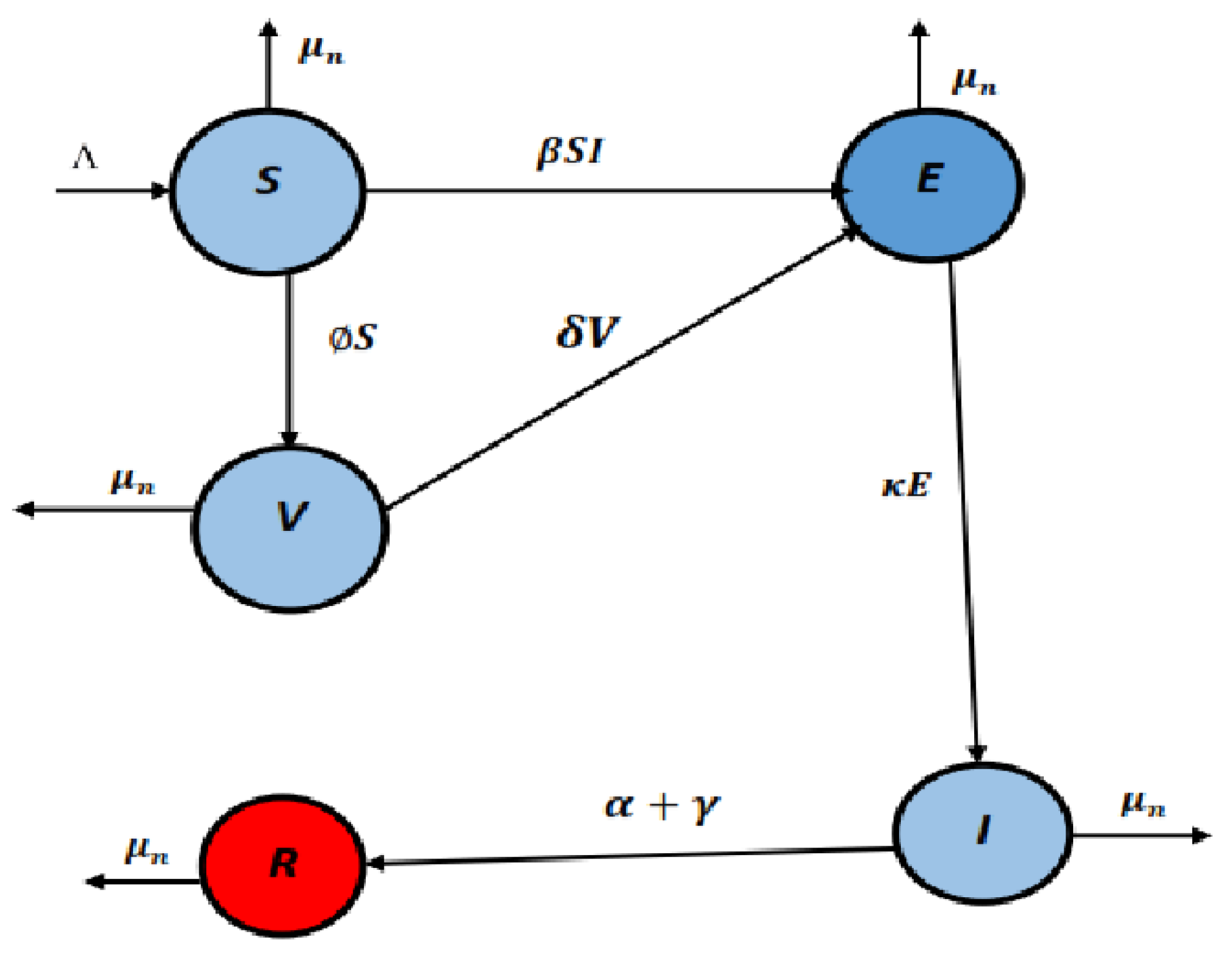
2. Formulation of the Model

Researchers [48] formulated a simple susceptible exposed infected and recovered (SEIR) model for the conjunctivitis virus of four compartments, and carried out a global and local stability analysis for the mentioned model. In the same way, authors [49] have extended the aforesaid model by incorporating the vaccinated class for the conjunctivitis virus with recovered individuals without medication. The mentioned model is described as follows:

$$\left\{\begin{array}{cc}\hfill & {\displaystyle \frac{dS\left(\theta \right)}{d\theta }}=\Lambda -\beta IS-{\mu }_{n}S\hfill \\ & {\displaystyle \frac{dE\left(\theta \right)}{d\theta }}=\beta IS-(\varphi +{\mu }_n)E,\hfill \\ & {\displaystyle \frac{dV\left(\theta \right)}{d\theta }}=\varphi E-(\kappa +{\mu }_n)V,\hfill \\ & {\displaystyle \frac{dI\left(\theta \right)}{d\theta }}=\kappa V-(\alpha +\gamma +{\mu }_n)I,\hfill \\ & {\displaystyle \frac{dR\left(\theta \right)}{d\theta }}=(\alpha +\gamma )I-{\mu }_{n}R,\hfill \end{array}\right.$$

(1)

with the initial conditions given as follows:

$$S\left(0\right)=S_0,E\left(0\right)=E_0,V\left(0\right)=V_0,I\left(0\right)=I_0,R\left(0\right)=R_0.$$

(2)

The model (1) is referred to as SEVIR for brevity. The model consists of five different compartments. The compartment “S” corresponds to the susceptible individuals, the compartment “E” indicates the exposed individuals, the compartment “V” indicates vaccinated individuals, the compartment “I” corresponds to conjunctivitis-infected individuals, and the compartment “R” indicates the recovered class of the population. Under the framework of the $ABC$ fractional derivative, the authors examined the aforementioned model for qualitative theory and a semi-analytical solution. They used the Samudu transform for the computation of solutions corresponding to different compartments. Also, they deduced some results by using the flip bifurcation procedure. Since the mentioned $ABC$ operator has been identified for some shortcomings and therefore for sophisticated mathematical analysis, the theory of fractals and fractional differential operators is the most effective. Therefore, we applied the fractals and fractional derivative to deduce the existence theory and numerical analysis of the considered model. The aforementioned model will be examined for existence theory by using a fixed point approach, for Ulam–Hyers stability by using the tools of nonlinear numerical functional analysis, and numerical analysis based on the Adam Bashforth method. Here, we remark that the mentioned numerical method is a powerful tool and has been used very effectively in the literature. The convergence and stability analyses of the said method, for classical as well as fractal fractional derivatives, were given in [50,51] recently.

Since the model (1) seems inconsistent, we therefore modified and investigated it under the fractal fractional derivative of order $\sigma ,\xi \in (0,1]$ by using $\Lambda =n{\beta }_n.$ Let $\lambda$ be used for recruitment rate, and $\beta$ for the transmission rate for acute hemorrhagic conjunctivitis spread from person to person. $\gamma$ denotes the recovery rate and ${\mu }_n$ is the natural death in all classes, and $\delta$ stands for the rate of vaccinated class in those exposed to become infected. In addition, the notation $\kappa$ shows the rate of incident from the vaccinated class to the infected class, while $\rho$ denotes the incidence rate for recovered individuals, $\alpha$ stands for the incidence rate for recovered measure, and $\varphi$ represents the incubation rate for acute hemorrhagic conjunctivitis. The notation n is used for the total population. Keeping in mind the given notations, we reformulate the model (1) under the fractal fractional derivatives as follows:

$$\left\{\begin{array}{cc}\hfill {}^{\mathrm{FAB}}\mathrm{D}_{0^{+}}^{\sigma ,\xi }S\left(\theta \right)& =\Lambda -\beta IS-\varphi S-{\mu }_{n}S,\hfill \\ \hfill {}^{\mathrm{FAB}}\mathrm{D}_{0^{+}}^{\sigma ,\xi }V\left(\theta \right)& =\varphi S-\delta V-{\mu }_{n}V,\hfill \\ \hfill {}^{\mathrm{FAB}}\mathrm{D}_{0^{+}}^{\sigma ,\xi }E\left(\theta \right)& =\beta SI+\delta V-(\kappa +{\mu }_n)E,\hfill \\ \hfill {}^{\mathrm{FAB}}\mathrm{D}_{0^{+}}^{\sigma ,\xi }I\left(\theta \right)& =\kappa E-(\alpha +\gamma +{\mu }_n)I,\hfill \\ \hfill {}^{\mathrm{FAB}}\mathrm{D}_{0^{+}}^{\sigma ,\xi }R\left(\theta \right)& =(\alpha +\gamma )I-{\mu }_{n}R.\hfill \end{array}\right.$$

(3)

and the initial conditions are defined as:

$$S\left(0\right)=S_0,E\left(0\right)=E_0,V\left(0\right)=V_0,I\left(0\right)=I_0,R\left(0\right)=R_0.$$

(4)

If we put $\sigma \in (0,1]$ and $\xi =1$, the corresponding model reduces to a fractional order model (3). If $\sigma =1$ and $\xi \in (0,1]$, we obtain the model (3) in fractal form. In both cases, the model studied in (1) becomes a special case of our model. Also, there was inconsistency in the model (1) studied by authors; we have modified and corrected the inconsistency. In fact, fractal fractional derivatives are a non-Newtonian generalization of the classical and traditional fractional derivatives. Therefore, taking the model (1) under the fractal fractional derivative is an alternative modeling approach. Keeping the usability of the aforesaid area, the mentioned disease model was not investigated previously in detail. Therefore, we needed to improve the model by removing the inconsistency in (1) and reformulate it under the fractal fractional derivative to establish some comprehensive results devoted to the existence theory and numerical analysis.

The parameters used in the model with numerical values are described as follows in

Table 1. The parameters and numerical values [49].

Parameters	Numerical Value	Parameters	Value
$\Lambda$	$0.00004215\times 2000$	$\kappa$	$0.0004$
$\beta$	$0.001$	$\rho$	$0.0000008$
$\gamma$	$0.00321$	$\alpha$	$0.08$
${\mu }_n$	R $0.000004215$	$\varphi$	$0.03$
$\delta$	$0.000004215$ (assumed)	n	2000

:

We will use functional analysis techniques and fixed point theory for existence theory and stability analysis. Lagrange’s interpolation technique will serve as the foundation for the numerical method used to build the approximate solution. The Figure 1 provides a description of the previously discussed model Equation (3).

3. Basic Results and Tools

To proceed further in this work, we need to recollect some required tools from [21,31,37,39]. Let $\mathbf{J}=[0,\mathbf{T}]$, and $\Omega =C(\mathbf{J},R)$ is the Banach space under the norm described by $\parallel \mathrm{U}\parallel ={sup}_{\theta \in \mathbf{J}}\left|\mathrm{U}\left(\theta \right)\right|.$

Definition 1. 

The R-L fractional integral with order $\sigma \in (0,1]$ can be described as:

$${}^{RL}\mathbf{I}^{\sigma }\mathrm{U}\left(\theta \right)={\displaystyle \frac{1}{\Gamma \left(\sigma \right)}}{\int }_0^{\theta }{(\theta -s)}^{\sigma -1}\mathrm{U}\left(s\right)ds,\theta \in [0,T].$$

Definition 2. 

The R-L fractional order derivative with order $\sigma \in (0,1]$ for $\mathrm{U}\in \Omega$ can be described as:

$${\mathrm{D}}_{0+}^{\sigma }\mathrm{U}\left(\theta \right)={\displaystyle \frac{1}{\Gamma (1-\sigma )}}{\displaystyle \frac{\mathrm{d}}{\mathrm{d}\theta }}{\int }_0^{\theta }{(\theta -\mathrm{s})}^{\sigma -1}\mathrm{U}\left(\mathrm{s}\right)\mathrm{d}\mathrm{s}.$$

Definition 3. 

The Caputo fractional order derivative with order $\sigma \in (0,1]$ for $\mathrm{U}\in \Omega$ is defined by

$${}^C\mathrm{D}_{0+}^{\sigma }\mathrm{U}\left(\theta \right)={\displaystyle \frac{1}{\Gamma (1-\sigma )}}{\int }_0^{\theta }{(\theta -\mathrm{s})}^{\sigma -1}{\mathrm{U}}^{\prime }\left(\mathrm{s}\right)\mathrm{d}\mathrm{s}.$$

Definition 4. 

The Atangana–Baleanu fractional integral with order $\sigma >0,$ of a function $\mathrm{U}\in \Omega$ can be described as

$${⠀}^{AB}{\mathbf{I}}_{0^{+}}^{\sigma }\mathrm{U}\left(\theta \right)={\displaystyle \frac{1-\sigma }{M\left(\sigma \right)}}\mathrm{U}\left(\theta \right)+{\displaystyle \frac{\sigma }{\Gamma \left(\sigma \right)M\left(\sigma \right)}}{\int }_0^{\theta }{(\theta -s)}^{\sigma -1}\mathrm{U}\left(s\right)dx,$$

such that the integral on the right side exists and is bounded.

Definition 5. 

The ABC differentiation with order $\sigma \in (0,1]$ of a differentiable function $\mathrm{U}\in {\mathrm{H}}^1(0,\mathrm{T})$ is defined by

$${}^{ABC}\mathrm{D}_0^{\sigma }\mathrm{U}\left(\theta \right)={\displaystyle \frac{M\left(\sigma \right)}{(1-\sigma )}}{\int }_0^{\theta }{E}_{\sigma }[-{\displaystyle \frac{\sigma }{1-\sigma }}{(\theta -s)}^{\sigma }]{\mathrm{U}}^{\prime }\left(s\right)dx,$$

where $M(·)$ is called normalized function.

Definition 6. 

Fractal-type arbitrary order integral of order $\sigma >0$ is defined as follows:

$${}^F\mathbf{I}_{0^{+}}^{\sigma }\mathrm{U}\left(\theta \right)=\sigma {\int }_0^{\theta }{s}^{\sigma -1}\mathrm{U}\left(s\right)ds.$$

(5)

Definition 7. 

Fractal fractional Atangana–Baleanu (FAB) integral with fractal order $\xi \in (0,1],$ and fractional order $\sigma \in (0,1]$ is defined as follows:

$${}^{FAB}\mathbf{I}_{0^{+}}^{\sigma ,\xi }\mathrm{U}\left(\theta \right)={\displaystyle \frac{\xi (1-\sigma ){\theta }^{\xi -1}}{M\left(\sigma \right)}}\mathrm{U}\left(\theta \right)+{\displaystyle \frac{\sigma \xi }{\Gamma \left(\sigma \right)M\left(\sigma \right)}}{\int }_0^{\theta }{(\theta -s)}^{\sigma -1}{s}^{\xi -1}\mathrm{U}\left(s\right)ds.$$

Definition 8. 

Fractal fractional $ABC$ derivative with fractal order $\xi \in (0,1],$ and fractional order $\sigma \in (0,1]$ is defined as follows:

$${}^{FAB}\mathbf{D}_0^{\sigma ,\xi }\mathrm{U}\left(\theta \right)={\displaystyle \frac{M\left(\sigma \right)}{(1-\sigma )}}{\int }_0^{\theta }{E}_{\sigma }[-{\displaystyle \frac{\sigma }{1-\sigma }}{(\theta -s)}^{\sigma }]{\displaystyle \frac{du\left(s\right)}{d{s}^{\xi }}}ds.$$

Lemma 1. 

If $\mathbf{X}\in L[0,T]$ and $\mathbf{X}\left(0\right)=0$, then the solution of

$$\begin{array}{ccc}\hfill {⠀}^{FAB}{D}^{\sigma ,\xi }\mathrm{U}\left(\theta \right)& =& \mathbf{X}\left(\theta \right),\mathit{with}\sigma \in (0,1],\hfill \\ \hfill \mathrm{U}\left(0\right)& =& {\mathrm{U}}_0,\hfill \end{array}$$

is described as follows:

$$\mathrm{U}\left(\theta \right)={\mathrm{U}}_0+{\displaystyle \frac{\xi (1-\sigma ){\theta }^{\xi -1}}{M\left(\sigma \right)}}x\left(\theta \right)+{\displaystyle \frac{\sigma \xi }{\Gamma \left(\sigma \right)M\left(\sigma \right)}}{\int }_0^{\theta }{(\theta -s)}^{\sigma -1}{s}^{\xi -1}\mathbf{X}\left(s\right)ds.$$

4. Some Basic Results

4.1. Positivity and Boundedness

In this regard, we deduce the results as follows:

Theorem 1. 

If the initial conditions $S\left(0\right)>0,V\left(0\right)\ge 0,E\left(0\right)\ge 0,I\left(0\right)\ge 0,$ and $R\left(0\right)\ge 0,$ such that the solutions of the model represented by $\left(S\right(\theta ),V(\theta ),E(\theta ),I(\theta ),R(\theta \left)\right)$ with non-negative initial data remain non-negative for all time $\theta >0.$ Further, the solution is bounded and lies in the feasible region given by

$$▵=\{(S,V,E,I,R)\in {\mathcal{R}}_{+}^5:S+V+E+I+R\le {\displaystyle \frac{\Lambda }{{\mu }_n}}\}.$$

Proof. 

We set $\Omega =sup\{\theta >0:S(\theta )>0,V(\theta )>0,E(\theta )>0,I(\theta )>0,R(\theta )>0\in [0,T\left]\right\},$ for all time $T>0$. From the first equation of model (3) under the classical derivatives, it follows that

$$\begin{array}{ccc}\hfill {\displaystyle \frac{dS}{d\theta }}& =& \Lambda +{\delta }_{2}S-\beta IS-\varphi S-{\mu }_{n}S\hfill \\ & \ge & -(\varphi +{\mu }_n)S.\hfill \end{array}$$

(6)

On solving (6), we obtain

$$S\left(\theta \right)\ge S\left(0\right)exp(-(\varphi +{\mu }_n)\theta )>0,\forall \theta >0.$$

Hence, it is trivial that $S\left(T\right)>0$. Therefore, $S\left(\theta \right)>0,\forall \theta >0.$ In the same way, we can prove for other equations of model (3) that $V\left(\theta \right)>0,E\left(\theta \right)>0,I\left(\theta \right)>0,$ and $R\left(\theta \right)>0,$ for all $\theta >0$. We know that

$$n=S+E+V+I+R.$$

(7)

Taking the derivative of (7), we have

$$\begin{array}{ccc}\hfill {\displaystyle \frac{dn}{d\theta }}& =& {\displaystyle \frac{dS}{d\theta }}+{\displaystyle \frac{dV}{d\theta }}+{\displaystyle \frac{dE}{d\theta }}+{\displaystyle \frac{dI}{d\theta }}+{\displaystyle \frac{dR}{d\theta }}\hfill \\ & \le & \Lambda -{\mu }_{n}n.\hfill \end{array}$$

On solving, we obtain

$$n\left(\theta \right)={\displaystyle \frac{\Lambda }{{\mu }_n}}+n\left(0\right)exp(-{\mu }_n\theta ).$$

At $\theta \to 0$ implies that

$$n\left(\theta \right)\to {\displaystyle \frac{\Lambda }{{\mu }_n}}.$$

   □

4.2. Equilibrium Points and Reproduction Number

The disease-free equilibrium (DFE) and endemic equilibrium (EE) points have been calculated as follows:

$${\mathcal{E}}_0=({\displaystyle \frac{\Lambda }{(\varphi +{\mu }_n)}},{\displaystyle \frac{\varphi \Lambda }{({\mu }_n+\varphi )({\mu }_n+\delta )}},0,0,0)$$

and there exist two EE points

$${\mathcal{E}}_1^{*}=(S_1^{*},V_1^{*},E_1^{*},.I_1^{*},R_1^{*}),{\mathcal{E}}_2^{*}=(S_2^{*},V_2^{*},E_2^{*},I_2^{*},R_2^{*}),$$

where we use for simplicity that

$$\lambda =\kappa \beta \Lambda (\delta +{\mu }_n),\omega =(\kappa +{\mu }_n)(\alpha +\gamma +{\mu }_n)(\delta +{\mu }_n),$$

such $A=\omega (\varphi +{\mu }_n)-\lambda ,B=\beta \omega ,C=\kappa \delta \Lambda \varphi ,$ then from (3), we have

$$\begin{array}{c}\hfill \Lambda -\beta I^{*}{S}^{*}-\varphi S^{*}-{\mu }_n{S}^{*}=0,\\ \hfill \varphi S^{*}-\delta V^{*}-{\mu }_n{V}^{*}=0,\\ \hfill \beta S^{*}{I}^{*}+\delta V^{*}-(\kappa +{\mu }_n)E^{*}=0,\\ \hfill \kappa E^{*}-(\alpha +\gamma +{\mu }_n)I^{*}=0,\\ \hfill (\alpha +\gamma )I^{*}-{\mu }_n{R}^{*}=0.\end{array}$$

(8)

From system (8), we have

$$\begin{array}{c}\hfill R^{*}={\displaystyle \frac{(\alpha +\gamma )I^{*}}{{\mu }_n}},E^{*}={\displaystyle \frac{(\alpha +\gamma +{\mu }_n)I^{*}}{\kappa }},\\ \hfill V^{*}={\displaystyle \frac{(\varphi -{\mu }_n)}{\delta }}{S}^{*},S^{*}={\displaystyle \frac{\Lambda }{\beta I^{*}+\varphi +{\mu }_n}}.\end{array}$$

(9)

In view of (9), we have

$$\begin{array}{c}\hfill A{\left[I^{*}\right]}^2+B{I}^{*}-C=0\end{array}$$

which gives

$$\begin{array}{c}\hfill I^{*}={\displaystyle \frac{-B\pm \sqrt{B^2-4AC}}{2A}}.\end{array}$$

(10)

Using the two roots of (9) and (10), we obtain the required EE points.

The basic ratio ${\mathcal{R}}_0$ has been computed by using the next-generation-matrix method. The said procedure has been studied in detail by researchers. By following the procedures mentioned, given by the following formula mentioned in [52,53], we compute the basic reproductive number as:

$${\mathcal{R}}_0={\displaystyle \frac{\Lambda \beta \kappa }{{\mu }_n(\kappa +{\mu }_n)(\alpha +\gamma +{\mu }_n)(\varphi +{\mu }_n)}}.$$

It has been shown that the disease-free equilibrium point of the proposed model is asymptotically stable if ${\mathcal{R}}_0\le 1$ and unstable if ${\mathcal{R}}_0>1$. Since the basic reproduction number indicates how many secondary infections, under typical behavioural patterns, an infected individual should cause in a population of hosts that are fully susceptible. Thus, ${\mathcal{R}}_0$ is a constant that accurately characterizes the initial phases of an epidemic brought on by a new virus. The values of ${\mathcal{R}}_0$ depends upon the parameter values. If ${\mathcal{R}}_0<1$, it shows that the infection is going to decrease and the equilibrium of the disease-free type will be locally asymptotically stable. But if ${\mathcal{R}}_0>1$, it shows an increase in infection in society. Hence, the value of ${\mathcal{R}}_0$ plays an important role in investigating such dynamical behaviour of the transmission of disease in a community. Against different values of parameters, we see that ${\mathcal{R}}_0<1$, as shown in Figure 2. In Figure 2a, we observe that as $\alpha$ decreases and ${\mu }_n$ decreases, the reproduction number increases but never exceeds 1. In the same way, in Figure 2b, as $\beta$, and $\Lambda$ decrease, the value of ${\mathcal{R}}_0$ increases but does not exceed 1. In addition, with the decrease in $\mu$ and $\gamma$ in Figure 2c, the value of ${\mathcal{R}}_0$ never exceeds 1. From Figure 2d, as we see that $\mu$ and $\Lambda$ decrease, the reproductive number values do not exceed 1. The different colors represent the difference between density plots of ${\mathcal{R}}_0$ against different values of the given parameters.

Theorem 2. 

If ${\mathcal{R}}_0<1$, then the DFE point is locally asymptotically stable.

Proof. 

The Jacobin matrix at the DFE point

$${\mathcal{E}}_0=({\displaystyle \frac{\Lambda }{(\varphi +{\mu }_n)}},{\displaystyle \frac{\varphi \Lambda }{({\mu }_n+\varphi )({\mu }_n+\delta )}},0,0,0)$$

of model (3) is given by

$$J\left({\mathcal{E}}_0\right)=\left(\begin{array}{ccccc}-(\varphi +{\mu }_n)& 0& 0& {\displaystyle \frac{-\beta \Lambda }{\varphi +{\mu }_n}}& 0\\ \varphi & -(\delta +{\mu }_n)& 0& 0& 0\\ 0& 0& -(\kappa +{\mu }_n)& {\displaystyle \frac{\beta \Lambda }{\varphi +{\mu }_n}}& 0\\ 0& 0& \kappa & -(\alpha +\gamma +{\mu }_n)& 0\\ 0& 0& 0& (\alpha +\gamma )& -{\mu }_n\end{array}\right).$$

We obtain the characteristic equation by using the $J\left({\mathcal{E}}_0\right)$

$$\begin{array}{c}\hfill (\lambda +(\varphi +{\mu }_n))(\lambda +{\mu }_n)[{\lambda }^3+a_1{\lambda }^2+a_2\lambda +a_3]=0,\end{array}$$

(11)

where $a_i,i=1,2,3$ are given by

$$\begin{array}{ccc}\hfill a_1& =& \delta +\alpha +\gamma +\kappa +3{\mu }_n,\hfill \\ \hfill a_2& =& (\kappa +{\mu }_n)(\alpha +\gamma +{\mu }_n)+\delta +{\mu }_n+{\displaystyle \frac{\kappa \beta \Lambda }{\varphi +{\mu }_n}},\hfill \\ \hfill a_3& =& (\delta +{\mu }_n)(\kappa +{\mu }_n)(\alpha +\gamma +{\mu }_n)+{\displaystyle \frac{1}{(\varphi +{\mu }_n)(\delta +{\mu }_n)}}[1-{\mathcal{R}}_0].\hfill \end{array}$$

We see that ${\lambda }_1=-(\varphi +{\mu }_n),{\lambda }_2=-{\mu }_n$ from (11), both are negative real parts. But the other three eigenvalues have negative real parts if the remaining three eigenvalues have negative real parts; if the Routh–Hewritz criteria [54] holds, that is $a_1>0,a_3>0,$ and $a_1{a}_2>a_3$. But $a_1{a}_2>a_3$ if ${\mathcal{R}}_0<1$. Hence, the DFE point of model (3) is locally asymptotically stable.    □

To show that DFE point is globally asymptotically stable, we apply the Castillo Chavez method [55]. Therefore, by reducing the model (3) to

$$\begin{array}{ccc}\hfill {\displaystyle \frac{dU}{dt}}& =& L(U,Z),\hfill \\ \hfill {\displaystyle \frac{dV}{dt}}& =& M(U,Z),\hfill \end{array}$$

(12)

where $U=(S,V,R)\in R^3$ the uninfected classes and $Z=(E,I)\in R^2,$ the infected ones. Now the DFE is given as ${\mathcal{E}}_0=(U^0,0)$, therefore the existence of a globally asymptotically stable DFE point depends on the given conditions:

• if ${\displaystyle \frac{dU}{dt}}=L(U^0,0)$, then $E^0$ is globally asymptotically stable.
• $M(U,Z)=WU-\overline{M}(U,Z),$ where $\overline{M}(U,Z)\ge 0$, for $(U,V)\in \Omega$, while $W=D_{Z}M(U^0,0)$ is an M-matrix, and $\Omega$ is the feasible region.

Lemma 2 

([55]). The DFE point ${\mathcal{E}}_0$ of a model is globally asymptotically stable if the above two conditions hold.

Theorem 3. 

If ${\mathcal{R}}_0<1$, then the DFE is globally asymptotically stable, and if ${\mathcal{R}}_0>1$, then the DFE is unstable.

Proof. 

To deduce the aforementioned conditions, let ${\mathcal{E}}_0=\left(U^0\right),$ where

$$U^0=\left({\displaystyle \frac{\Lambda }{(\varphi +{\mu }_n)}},{\displaystyle \frac{\varphi \Lambda }{({\mu }_n+\varphi )({\mu }_n+\delta )}},0\right).$$

Then, we have

$$\begin{array}{ccc}\hfill {\displaystyle \frac{dU}{dt}}& =& L(U,Z)\hfill \\ & =& \left(\begin{array}{c}\Lambda -\beta IS-(\varphi +{\mu }_n)S\\ \varphi S-(\delta +{\mu }_n)V\\ (\alpha +\gamma )I-{\mu }_{n}R\end{array}\right),\hfill \end{array}$$

from then on, using $S=S^0,V=V^0,R=R^0$ and $L(U,Z)=0$, we have

$$\begin{array}{c}\hfill L(U,0)=\left(\begin{array}{c}\Lambda --(\varphi +{\mu }_n)S^0\\ \varphi S^0-(\delta +{\mu }_n)V^0\\ -{\mu }_n{R}^0\end{array}\right)=0.\end{array}$$

At $t\to \infty$, we see that $U\to U^0$, Therefore, $U=U^0$ is globally asymptotically stable. In the same way, for the other condition, we can prove that

$$WU-\overline{M}(U,Z)=\left(\begin{array}{cc}-(\kappa +{\mu }_n)& {\displaystyle \frac{\beta \Lambda }{{\mu }_n+\varphi }}\\ -(\alpha +\gamma +{\mu }_n)& \kappa \end{array}\right)\left(\begin{array}{c}E\\ I\end{array}\right)-\left(\begin{array}{c}{\displaystyle \frac{\delta \varphi \Lambda }{({\mu }_n+\varphi )(\delta +{\mu }_n)}}\\ 0\end{array}\right),$$

where

$$W=\left(\begin{array}{cc}-(\kappa +{\mu }_n)& {\displaystyle \frac{\beta \Lambda }{{\mu }_n+\varphi }}\\ -(\alpha +\gamma +{\mu }_n)& \kappa \end{array}\right),\overline{M}(U,V)=\left(\begin{array}{c}{\displaystyle \frac{\delta \varphi \Lambda }{({\mu }_n+\varphi )(\delta +{\mu }_n)}}\\ 0\end{array}\right).$$

We see that ${\displaystyle \frac{\delta \varphi \Lambda }{({\mu }_n+\varphi )(\delta +{\mu }_n)}}>0$, hence $\overline{M}(U,Z)\ge 0.$ Therefore, both conditions for global stability hold, and hence, the DFE of model (3) is globally asymptotically stable.    □

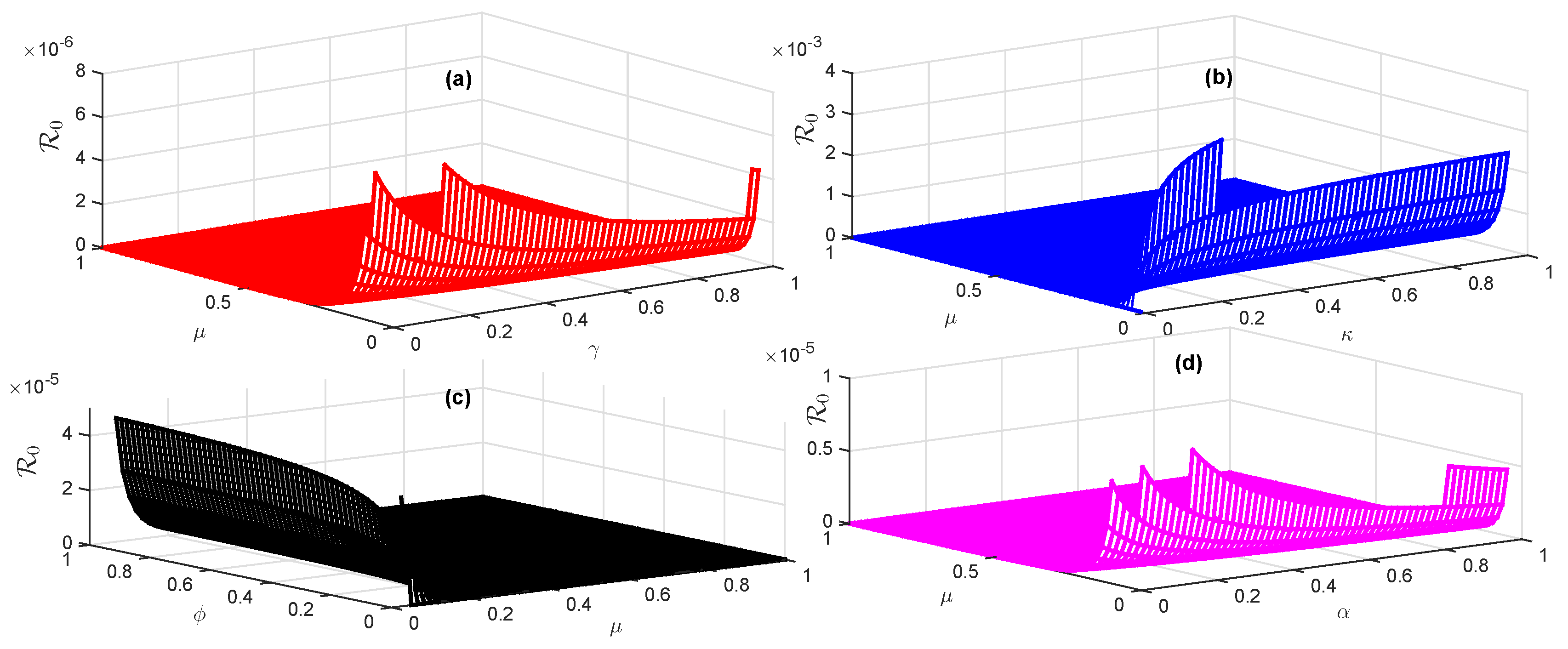
4.3. Sensitivity Analysis

Sensitivity analysis is used to identify the parameters that are useful in limiting the spread of infectious disease. Even if the calculation of forward sensitivity analysis grows laborious for complicated biological models, it is nevertheless regarded as an essential part of disease modelling. Researchers in pedagogical disease have paid close attention to basic reproductive number ${\mathcal{R}}_0$ sensitivity analysis. As an important contribution in this regard, we refer to [56]. There are three methods given by researchers to study the sensitivity analysis, which are listed as follows:

• Linearizing the considered model.
• Latin hypercube sampling method.
• Direct differentiation method.

In addition, the sensitivity index is computed via using the direct differentiation formula [57] given by ${\mathbf{S}}_p^{{\mathcal{R}}_0}={\displaystyle \frac{p}{{\mathcal{R}}_0}}{\displaystyle \frac{\partial {\mathcal{R}}_0}{\partial p}},$ where p stands for parameter. We compute the corresponding indices as follows using the said formula:

$$\begin{array}{ccc}\hfill {\mathbf{S}}_{\Lambda }^{{\mathcal{R}}_0}& =& {\displaystyle \frac{\Lambda }{{\mathcal{R}}_0}}{\displaystyle \frac{\partial {\mathcal{R}}_0}{\partial \Lambda }}=1>0,\hfill \\ \hfill {\mathbf{S}}_{\beta }^{{\mathcal{R}}_0}& =& {\displaystyle \frac{\beta }{{\mathcal{R}}_0}}{\displaystyle \frac{\partial {\mathcal{R}}_0}{\partial \beta }}=1>0,\hfill \\ \hfill {\mathbf{S}}_{\kappa }^{{\mathcal{R}}_0}& =& {\displaystyle \frac{\kappa }{{\mathcal{R}}_0}}{\displaystyle \frac{\partial {\mathcal{R}}_0}{\partial \kappa }}=4.395141\times {10}^{-9}>0,\hfill \\ \hfill {\mathbf{S}}_{{\mu }_n}^{{\mathcal{R}}_0}& =& {\displaystyle \frac{{\mu }_n}{{\mathcal{R}}_0}}{\displaystyle \frac{\partial {\mathcal{R}}_0}{\partial {\mu }_n}}=-7.87654\times {10}^{-6}<0,\hfill \\ \hfill {\mathbf{S}}_{\alpha }^{{\mathcal{R}}_0}& =& {\displaystyle \frac{\alpha }{{\mathcal{R}}_0}}{\displaystyle \frac{\partial {\mathcal{R}}_0}{\partial \alpha }}=-6.98764\times {10}^{-6}<0,\hfill \\ \hfill {\mathbf{S}}_{\gamma }^{{\mathcal{R}}_0}& =& {\displaystyle \frac{\gamma }{{\mathcal{R}}_0}}{\displaystyle \frac{\partial {\mathcal{R}}_0}{\partial \gamma }}=-5.013707\times {10}^{-6}<0,\hfill \\ \hfill {\mathbf{S}}_{\varphi }^{{\mathcal{R}}_0}& =& {\displaystyle \frac{\varphi }{{\mathcal{R}}_0}}{\displaystyle \frac{\partial {\mathcal{R}}_0}{\partial \varphi }}=-8.013707\times {10}^{-6}<0,\hfill \end{array}$$

(13)

The values which have been computed in (13) for the sensitivity index against various parameters demonstrate that the reproduction number ${\mathcal{R}}_0$ is positively influenced by the parameters $\Lambda ,\beta ,\kappa$. This implies that a 100% increase or decrease in these parameters will result in a 100% increase or decrease in the reproduction number, which will be 100 percent, 100 percent, and $4.395141\times {10}^{-7}$ percent, respectively. However, the index for parameters ${\mu }_n,\alpha ,\gamma ,$ and $\varphi$ shows that a 100% increase in their values will result in $7.87654\times {10}^{-4},6.98764\times {10}^{-4},5.013707\times {10}^{-4},8.013707\times {10}^{-4}$ percent decreases in the values of reproduction number ${\mathcal{R}}_0$.

5. Existence Theory

Existence theory is one of the important aspect of differential equations. Therefore, in this section, some results will be formulated about the qualitative behaviour of the model. Let us assume the following:

$$\left\{\begin{array}{cc}\hfill {\Psi }_1(\theta ,S,E,V,I,R)& =\Lambda -\beta IS-{\mu }_{n}S-\varphi S,\hfill \\ \hfill {\Psi }_2(\theta ,S,E,V,I,R)& =\varphi S-\delta V-{\mu }_{n}V\hfill \\ \hfill {\Psi }_3(\theta ,S,E,V,I,R)& =\beta SI+\delta V-(\kappa +{\mu }_n)E,\hfill \\ \hfill {\Psi }_4(\theta ,S,E,V,I,R)& =\kappa E-(\alpha +\gamma +{\mu }_n)I,\hfill \\ \hfill {\Psi }_5(\theta ,S,E,V,I,R)& =(\alpha +\gamma )I-{\mu }_{n}R.\hfill \end{array}\right.$$

(14)

Using system (14), system (3), with $\sigma \in (0,1]$ may be simply expressed as:

$$\left\{\begin{array}{c}{⠀}^{\mathrm{FAB}}{\mathrm{D}}_{0^{+}}^{\sigma ,\xi }\mathrm{U}\left(\theta \right)=\mathbf{F}(\theta ,\mathrm{U}\left(\theta \right)),\theta \in [0,\mathbf{T}],\hfill \\ ⠀\mathrm{U}\left(0\right)={\mathrm{U}}_0,\hfill \end{array}\right.$$

(15)

where

$$\mathrm{U}\left(\theta \right)=\left\{\begin{array}{cc}& S\left(\theta \right),\hfill \\ & V\left(\theta \right),\hfill \\ & E\left(\theta \right),\hfill \\ & I\left(\theta \right),\hfill \\ & R\left(\theta \right).\hfill \end{array}\right.,{\mathrm{U}}_0\left(\theta \right)=\left\{\begin{array}{cc}& S_0,\hfill \\ & V_0,\hfill \\ & E_0,\hfill \\ & I_0,\hfill \\ & R_0,\hfill \end{array}\right.,\mathbf{F}(\theta ,\mathrm{U}\left(\theta \right))=\left\{\begin{array}{cc}& {\Psi }_1(\theta ,S,E,V,I,R),\hfill \\ & {\Psi }_2(\theta ,S,E,V,I,R),\hfill \\ & {\Psi }_3(\theta ,S,E,V,I,R),\hfill \\ & {\Psi }_4(\theta ,S,E,V,I,R),\hfill \\ & {\Psi }_5(\theta ,S,E,V,I,R).\hfill \end{array}\right.$$

(16)

In view of the application of Lemma 1, the equivalent integral equation of problem (15) may be expressed as:

$$\mathrm{U}\left(\theta \right)={\mathrm{U}}_0+{\displaystyle \frac{\xi (1-\sigma ){\theta }^{\xi -1}}{M\left(\sigma \right)}}\mathbf{F}(\theta ,\mathrm{U}\left(\theta \right))+{\displaystyle \frac{\sigma \xi }{\Gamma \left(\sigma \right)M\left(\sigma \right)}}{\int }_0^{\theta }{(\theta -\mathrm{s})}^{\sigma -1}{\mathrm{s}}^{\xi -1}\mathbf{F}(\mathrm{s},\mathrm{U}\left(\mathrm{s}\right))\mathrm{d}\mathrm{s}.$$

(17)

Now, define the operator $\mathbf{G}:\Omega \to \Omega$ by:

$$\mathbf{G}\mathrm{U}\left(\theta \right)={\mathrm{U}}_0+{\displaystyle \frac{\xi (1-\sigma ){\theta }^{\xi -1}}{M\left(\sigma \right)}}\mathbf{F}(\theta ,\mathrm{U}\left(\theta \right))+{\displaystyle \frac{\sigma \xi }{\Gamma \left(\sigma \right)M\left(\sigma \right)}}{\int }_0^{\theta }{(\theta -\mathrm{s})}^{\sigma -1}{\mathrm{s}}^{\xi -1}\mathbf{F}(\mathrm{s},\mathrm{U}\left(\mathrm{s}\right))\mathrm{d}\mathrm{s}.$$

(18)

By splitting operator “$\mathbf{G}$” into two operators “${\mathbf{G}}_1$” and “${\mathbf{G}}_2$” as

$${\mathbf{G}}_1\mathrm{U}\left(\theta \right)={\mathrm{U}}_0+{\displaystyle \frac{\xi (1-\sigma ){\theta }^{\xi -1}}{M\left(\sigma \right)}}\mathbf{F}(\theta ,\mathrm{U}\left(\theta \right))$$

(19)

and

$${\mathbf{G}}_2\mathrm{U}\left(\theta \right)={\displaystyle \frac{\sigma \xi }{\Gamma \left(\sigma \right)M\left(\sigma \right)}}{\int }_0^{\theta }{(\theta -\mathrm{s})}^{\sigma -1}{\mathrm{s}}^{\xi -1}\mathbf{F}(\mathrm{s},\mathrm{U}\left(\mathrm{s}\right))\mathrm{d}\mathrm{s}.$$

(20)

From Equations (19) and (20), $\mathbf{G}\left(\mathrm{U}\right)$ can be written as:

$$\mathbf{G}\left(\mathrm{U}\right)={\mathbf{G}}_1\left(\mathrm{U}\right)+{\mathbf{G}}_2\left(\mathrm{U}\right).$$

(21)

Assume the following conditions hold:

(P₁)

Let, there exist two positive constants ${\mathbf{L}}_{\mathbf{G}}\mathrm{and}{\mathbf{C}}_{\mathbf{G}}>0$, such that

$$\left|\mathbf{F}(\theta ,\mathrm{U}\left(\theta \right))\right|\le {\mathbf{L}}_{\mathbf{G}}\left|\mathrm{U}\left(\theta \right)\right|+{\mathbf{C}}_{\mathbf{G}}.$$

(P₂)

Let there exist a positive constant, ${\mathbf{A}}_{\mathbf{G}}\mathrm{and}\mathrm{for}\mathrm{any}\mathrm{U},\overline{\mathrm{U}}\in \Omega ,$ such that

$$|\mathbf{F}(\theta ,\mathrm{U}\left(\theta \right))-\mathbf{F}(\theta ,\overline{\mathrm{U}}\left(\theta \right))|\le {\mathbf{A}}_{\mathbf{G}}|\mathrm{U}-\overline{\mathrm{U}}|.$$

Theorem 4. 

If the condition $\mathbf{A}=\left({\displaystyle \frac{{\mathbf{A}}_{\mathbf{G}}\xi (1-\sigma ){\mathrm{T}}^{\xi -1}}{M\left(\sigma \right)}}\right)<1$ holds together with the assumptions “${\mathbf{P}}_{\mathbf{1}}-{\mathbf{P}}_{\mathbf{2}}$", then Equation (15) has at least one solution.

Proof. 

Let $\mathrm{U},\overline{\mathrm{U}}\in \mathbf{S}$, then

$$\begin{array}{ccc}\hfill \parallel {\mathbf{G}}_{\mathbf{1}}\left(\mathrm{U}\right)-{\mathbf{G}}_{\mathbf{1}}\left(\overline{\mathrm{U}}\right)\parallel & =& \underset{\theta \in [0,\mathrm{T}]}{sup}\left\{\right|{\mathrm{U}}_0+\left({\displaystyle \frac{\xi (1-\sigma ){\theta }^{\xi -1}}{M\left(\sigma \right)}}\right)\mathbf{F}(\theta ,\mathrm{U}\left(\theta \right))\hfill \\ & & -\left[{\overline{\mathrm{U}}}_0+\left({\displaystyle \frac{\xi (1-\sigma ){\theta }^{\xi -1}}{M\left(\sigma \right)}}\right)\mathbf{F}(\theta ,\overline{\mathrm{U}}\left(\theta \right))\right]\left|\right\},\hfill \\ & \le & \underset{\theta \in [0,\mathrm{T}]}{sup}\left\{\left({\displaystyle \frac{{\mathbf{A}}_{\mathbf{G}}\xi (1-\sigma ){\theta }^{\xi -1}}{M\left(\sigma \right)}}\right)|\mathrm{U}\left(\theta \right)-\overline{\mathrm{U}}\left(\theta \right)|\right\},\hfill \\ & \le & \left({\displaystyle \frac{{\mathbf{A}}_{\mathbf{G}}\xi (1-\sigma ){\mathrm{T}}^{\xi -1}}{M\left(\sigma \right)}}\right)\parallel \mathrm{U}-\overline{\mathrm{U}}\parallel ,\hfill \\ & \le & \mathbf{A}\parallel \mathrm{U}-\overline{\mathrm{U}}\parallel .\hfill \end{array}$$

which yields that ${\mathbf{G}}_{\mathbf{1}}$ is a contraction. Additionally, if $\mathbf{S}=\{\mathrm{U}\in \Omega :\parallel \mathrm{U}\parallel \le \mathrm{r}\}\subset \Omega$ is a bounded and closed set, then

$$\begin{array}{ccc}\hfill \parallel {\mathbf{G}}_{\mathbf{2}}\left(\mathrm{U}\right)\parallel & =& \underset{\theta \in [0,\mathrm{T}]}{sup}\left\{\left|{\displaystyle \frac{\sigma \xi }{\Gamma \left(\sigma \right)M\left(\sigma \right)}}{\int }_0^{\theta }{(\theta -\mathrm{s})}^{\sigma -1}{\mathrm{s}}^{\xi -1}\mathbf{F}(\mathrm{s},\mathrm{U}\left(\mathrm{s}\right))\mathrm{d}\mathrm{s}\right|\right\},\hfill \\ & \le & {\displaystyle \frac{\sigma \xi \parallel \mathbf{F}\parallel }{M\left(\sigma \right)}}\underset{\theta \in [0,\mathrm{T}]}{sup}\left\{\left|{\int }_0^{\theta }{\displaystyle \frac{{(\theta -\mathrm{s})}^{\sigma -1}}{\Gamma \left(\sigma \right)}}{\mathrm{s}}^{\xi -1}\mathrm{d}\mathrm{s}\right|\right\},\hfill \\ & \le & \left({\displaystyle \frac{\sigma \Gamma (\xi +1){\mathrm{T}}^{\sigma +\xi -1}}{M\left(\sigma \right)\Gamma (\sigma +\xi )}}\right)({\mathbf{L}}_{\mathbf{G}}\parallel \mathrm{U}\parallel +{\mathbf{C}}_{\mathbf{G}}),\hfill \\ & <& \infty .\hfill \end{array}$$

Thus, ${\mathbf{G}}_{\mathbf{2}}$ is bounded and continuous. Additionally, if ${\theta }_1<{\theta }_2\in [0,\mathrm{T}],$ then

$$\begin{array}{ccc}\hfill \parallel {\mathbf{G}}_{\mathbf{2}}\mathrm{U}\left({\theta }_2\right)-{\mathbf{G}}_{\mathbf{2}}\mathrm{U}\left({\theta }_1\right)\parallel & =& \underset{{\theta }_1,{\theta }_2\in [0,\mathrm{T}]}{sup}\left\{{\displaystyle \frac{\sigma \xi }{\Gamma \left(\sigma \right)M\left(\sigma \right)}}\right|{\int }_0^{{\theta }_2}{({\theta }_2-\mathrm{s})}^{\sigma -1}{\mathrm{s}}^{\xi -1}\mathbf{F}(\mathrm{s},\mathrm{U}\left(\mathrm{s}\right))\mathrm{d}\mathrm{s}\hfill \\ & & -{\int }_0^{{\theta }_1}{({\theta }_1-\mathrm{s})}^{\sigma -1}{\mathrm{s}}^{\xi -1}\mathbf{F}(\mathrm{s},\mathrm{U}\left(\mathrm{s}\right))\mathrm{d}\mathrm{s}\left|\right\},\hfill \\ & \le & \left({\displaystyle \frac{\sigma \xi \parallel \mathbf{F}\parallel }{\Gamma \left(\sigma \right)M\left(\sigma \right)}}\right)|{\int }_0^{{\theta }_2}{({\theta }_2-\mathrm{s})}^{\sigma -1}{\mathrm{s}}^{\xi -1}\mathrm{d}\mathrm{s}-{\int }_0^{{\theta }_1}{({\theta }_1-\mathrm{s})}^{\sigma -1}{\mathrm{s}}^{\xi -1}\mathrm{d}\mathrm{s}|\hfill \\ & \le & \left({\displaystyle \frac{\sigma \Gamma (\xi +1)({\mathbf{L}}_{\mathbf{G}}\parallel \mathrm{U}\parallel +{\mathbf{C}}_{\mathbf{G}})}{M\left(\sigma \right)\Gamma (\sigma +\xi )}}\right)\left({\theta }_2^{\sigma +\xi -1}-{\theta }_1^{\sigma +\xi -1}\right)\to 0,\mathrm{as}{\theta }_1\to {\theta }_2.\hfill \end{array}$$

Hence, $“{\mathbf{G}}_{\mathbf{2}}”$ is equi-continuous, and $“{\mathbf{G}}_{\mathbf{2}}”$ is bounded. Therefore in view of Arzelá–Ascoli, and Krasnoselskii’s theorem, the model (15) has at least one solution.    □

Theorem 5. 

Under the assumption $“{\mathbf{P}}_{\mathbf{1}}”$, our considered problem has a unique solution if ${\mathbf{A}}^{\prime }=\left[\mathbf{A}+{\displaystyle \frac{\sigma \Gamma (\xi +1){\mathbf{A}}_{\mathbf{G}}{\mathrm{T}}^{\sigma +\xi -1}}{\Gamma (\sigma +\xi )M\left(\sigma \right)}}\right]<1$ holds.

Proof. 

By taking $\mathrm{U},\overline{\mathrm{U}}\in \mathbf{S}$, we have

$$\begin{array}{ccc}\hfill \parallel \mathbf{G}\left(\mathrm{U}\right)-\mathbf{G}\left(\overline{\mathrm{U}}\right)\parallel & =& \parallel {\mathbf{G}}_1\left(\mathrm{U}\right)+{\mathbf{G}}_2\left(\mathrm{U}\right)-({\mathbf{G}}_1(\overline{\mathrm{U}}+{\mathbf{G}}_2\left(\overline{\mathrm{U}}\right)\parallel \hfill \\ & \le & \parallel {\mathbf{G}}_1\left(\mathrm{U}\right)-{\mathbf{G}}_1\left(\overline{\mathrm{U}}\right)\parallel +\parallel {\mathbf{G}}_2\left(\mathrm{U}\right)-{\mathbf{G}}_2\left(\overline{\mathrm{U}}\right)\parallel \hfill \\ & \le & \mathbf{A}\parallel \mathrm{U}-\overline{\mathrm{U}}\parallel +{\displaystyle \frac{\sigma \xi }{\Gamma \left(\sigma \right)M\left(\sigma \right)}}\underset{\theta \in [0,\mathrm{T}]}{sup}\left\{\right|{\int }_0^{\theta }{(\theta -\mathrm{s})}^{\sigma -1}{\mathrm{s}}^{\xi -1}\mathbf{F}(\mathrm{s},\mathrm{U}\left(\mathrm{s}\right))\mathrm{d}\mathrm{s}\hfill \\ & & -\left({\int }_0^{\theta }{(\theta -\mathrm{s})}^{\sigma -1}{\mathrm{s}}^{\xi -1}\mathbf{F}(\mathrm{s},\overline{\mathrm{U}}\left(\mathrm{s}\right))\mathrm{d}\mathrm{s}\right)\left|\right\},\hfill \\ & \le & \mathbf{A}\parallel \mathrm{U}-\overline{\mathrm{U}}\parallel +{\displaystyle \frac{\sigma \xi {\mathbf{A}}_{\mathbf{G}}}{\Gamma \left(\sigma \right)M\left(\sigma \right)}}\parallel \mathrm{U}-\overline{\mathrm{U}}\parallel \underset{\theta \in [0,\mathrm{T}]}{sup}\left[{\int }_0^{\theta }{(\theta -\mathrm{s})}^{\sigma -1}{\mathrm{s}}^{\xi -1}\mathrm{d}\mathrm{s}\right],\hfill \\ & \le & \left[\mathbf{A}+{\displaystyle \frac{\sigma \Gamma (\xi +1)\xi {\mathbf{A}}_{\mathbf{G}}{\mathrm{T}}^{\sigma +\xi -1}}{\Gamma (\sigma +\xi )M\left(\sigma \right)}}\right]\parallel \mathrm{U}-\overline{\mathrm{U}}\parallel ,\hfill \\ & =& {\mathbf{A}}^{\prime }\parallel \mathrm{U}-\overline{\mathrm{U}}\parallel .\hfill \end{array}$$

where

$${\mathbf{A}}^{\prime }=\left[\mathbf{A}+{\displaystyle \frac{\sigma \Gamma (\xi +1){\mathbf{A}}_{\mathbf{G}}{\mathrm{T}}^{\sigma +\xi -1}}{\Gamma (\sigma +\xi )M\left(\sigma \right)}}\right].$$

We obtain the uniqueness result.    □

5.1. Ulam–Hyers Stability

Stability in mathematics is mainly concerned with the stability of dynamical system trajectories and solutions to differential equations under slight changes in its initial circumstances. For dynamical system and differential equations stability, this means that the solution curve does not change too much from its initial state due to small perturbations in the system. One of the important types of stability is Ulam–Hyer’s stability, which is particularly used for the convergence of approximate solutions of functional equations. The mentioned stability answered the basic question “under what conditions the approximate solutions are nearly equal to its exact solution of a functional equation?”. This concept was introduced for the first time by Ulam [58] and further generalized by Rassias [59]. Therefore, due to importance of the aforesaid stability, in this section, the model will be considered for Ulam–Hyers (U-H) stability.

The following definitions of Ulam–Hyers-type stability are recalled from [58,59,60]. For the definitions of the mentioned stability, let us define a general differential equation as follows:

$$\left\{\begin{array}{cc}\hfill {\mathrm{D}}_{0^{+}}^{\sigma }\mathrm{U}\left(\theta \right)& =\mathbf{F}(\theta ,\mathrm{U}(\theta \left)\right),\theta \in =[0,\mathrm{T}],\hfill \\ \hfill \mathrm{U}\left(0\right)& ={\mathrm{U}}_0.\hfill \end{array}\right.$$

(22)

5.2. Ulam–Hyer’s Stability

Definition 9. 

The solution of differential Equation (22) is Ulam–Hyers(U-H) stable, if for $ϵ>0$, there exists a constant $\mathbf{K}\in {\mathrm{R}}^{+}$ and for any solution $\mathrm{U}\in \Omega$ of the inequality

$$|{\mathrm{D}}_{0+}^{\sigma }\mathrm{U}\left(\theta \right)-\mathbf{F}(\theta ,\mathrm{U}\left(\theta \right))|\le ϵ,\mathit{for}\mathit{all}\theta \in [0,\mathrm{T}],$$

(23)

and unique solution $\overline{\mathrm{U}}\in \Omega$ of Equation (22), such that

$$|\mathrm{U}-\overline{\mathrm{U}}|\le \mathbf{K}ϵ,\mathit{for}\mathit{all}\theta \in [0,\mathrm{T}].$$

5.3. Generalized-Ulam–Hyers Stability

Definition 10. 

The solution of differential Equation (22) is generalized-Ulam–Hyers(g-U-H) stable, if there exists a continuous map $\Psi \in \mathrm{C}({\mathrm{R}}^{+},{\mathrm{R}}^{+})$ where $\Psi \left(0\right)=0$, such that for any solution $\mathrm{U}\in \Omega$ of the inequality (23) there exists a unique solution $\overline{\mathrm{U}}\in \Omega$ of Equation (22), such that

$$|\mathrm{U}-\overline{\mathrm{U}}|\le \Psi \left(ϵ\right),\mathit{for}\mathit{all}\theta \in [0,\mathrm{T}].$$

5.4. Ulam–Hyers–Rassias Stability

Definition 11. 

The solution of differential Equation (22) is Ulam–Hyers–Rassias(U-H-R) stable under $\psi \in \mathrm{C}[\mathbf{J},{\mathrm{R}}^{+}]$ if there exists $\mathbf{K}\in {\mathrm{R}}^{+}$, such that for every $ϵ>0$ and for any solution $\mathrm{U}\in \Omega$ of the inequality

$$|{\mathrm{D}}_{0+}^{\sigma }\mathrm{U}\left(\theta \right)-\mathbf{F}(\theta ,\mathrm{U}\left(\theta \right))|\le \psi \left(\theta \right)ϵ,\mathit{for}\mathit{all}\theta \in [0,\mathrm{T}],$$

(24)

there is a unique solution $\overline{\mathrm{U}}\in \Omega$ of Equation (22), such that

$$|\mathrm{U}-\overline{\mathrm{U}}|\le \mathbf{K}ϵ\psi \left(\theta \right),\mathit{for}\mathit{all}\theta \in [0,\mathrm{T}].$$

5.5. Generalized-Ulam–Hyers–Rassias Stability

Definition 12. 

The solution of differential Equation (22) is generalized-Ulam–Hyers–Rassias(g-U-H-R) stable, with respect to $\psi \in \mathrm{C}[J,{\mathrm{R}}^{+}]$ if there exists ${\mathbf{K}}_{\psi }\in {\mathrm{R}}^{+}$, such that for every $ϵ>0$ and for any solution $\mathrm{U}\in \Omega$ of the inequality (24) there is a unique solution $\overline{\mathrm{U}}\in \Omega$ of Equation (22), such that

$$|\mathrm{U}-\overline{\mathrm{U}}|\le {\mathbf{K}}_{\psi }\psi \left(\theta \right),\mathit{for}\mathit{all}\theta \in [0,\mathrm{T}].$$

Remark 1. 

A function $\overline{\mathrm{U}}$ is the solution of inequality (23), if a function $\chi \left(\theta \right)\in \mathrm{C}([0,\mathrm{T}];\mathrm{R})$ exist, such that

(I) 

$\left|\chi \right(\theta \left)\right|\le ϵ,\mathit{for}\mathit{all}\theta \in [0,\mathrm{T}].$

(II) 

${\mathrm{D}}^{\sigma }\overline{\mathrm{U}}\left(\theta \right)=\mathbf{F}(\theta ,\overline{\mathrm{U}}\left(\theta \right)+\chi \left(\theta \right),\mathit{for}\mathit{all}\theta \in [0,\mathrm{T}].$

Remark 2. 

A function $\overline{\mathrm{U}}$ is the solution of inequality (24), if a function $\chi \left(\theta \right)\in \mathrm{C}([0,\mathrm{T}];\mathrm{R})$ exist, such that

(I) 

$\left|\chi \right(\theta \left)\right|\le ϵ\psi ,\mathit{for}\mathit{all}\theta \in [0,\mathrm{T}].$

(II) 

${\mathrm{D}}^{\sigma }\overline{\mathrm{U}}\left(\theta \right)=\mathbf{F}(\theta ,\overline{\mathrm{U}}\left(\theta \right))+\chi \left(\theta \right),\mathit{for}\mathit{all}\theta \in [0,\mathrm{T}].$

Consider the corresponding perturbed problem of Equation (15) as

$$\left\{\begin{array}{cc}\hfill {}^{\mathrm{FAB}}\mathrm{D}_{0^{+}}^{\sigma ,\xi }\mathrm{U}\left(\theta \right)& =\mathbf{F}(\theta ,\mathrm{U}\left(\theta \right))+\chi \left(\theta \right),\theta \in \mathbf{J},\hfill \\ \hfill \mathrm{U}\left(0\right)& ={\mathrm{U}}_0.\hfill \end{array}\right.$$

(25)

Here, $\chi \left(\theta \right)\in C(\mathbf{J},\mathrm{R})$ such that for $ϵ>0$, $\left|\chi \right(\theta \left)\right||\le ϵ$. For any $\mathrm{U}$ solution of Equation (25), such that

$$\mathbf{G}\left(\mathrm{U}\right(\theta \left)\right)=\mathrm{U}\left(\theta \right)+\chi \left(\theta \right),$$

(26)

then the solution of Equation (25) is given as

$$\mathrm{U}\left(\theta \right)=\left\{\begin{array}{c}{\mathrm{U}}_0+{\displaystyle \frac{\xi (1-\sigma ){\theta }^{\xi -1}}{M\left(\sigma \right)}}[\mathbf{F}(\theta ,\mathrm{U}\left(\theta \right))+\chi \left(\theta \right)]\hfill \\ +{\displaystyle \frac{\sigma \xi }{\Gamma \left(\sigma \right)M\left(\sigma \right)}}{\int }_0^{\theta }{(\theta -\mathrm{s})}^{\sigma -1}{\mathrm{s}}^{\xi -1}[\mathbf{F}(\mathrm{s},\mathrm{U}\left(\mathrm{s}\right))+\chi \left(\mathrm{s}\right)]\mathrm{d}\mathrm{s}.\hfill \end{array}\right.$$

(27)

Using Equations (18) and (27), we have

$$\begin{array}{ccc}\hfill \left|\mathbf{G}\right(\mathrm{U}\left(\theta \right))-\mathrm{U}(\theta \left)\right|& \le & \left[{\displaystyle \frac{\xi (1-\sigma ){\mathrm{T}}^{\xi -1}}{M\left(\sigma \right)}}\right]ϵ+\left[{\displaystyle \frac{\sigma \Gamma (\xi +1){\mathrm{T}}^{\sigma +\xi -1}}{\Gamma (\sigma +\xi )M\left(\sigma \right)}}\right]ϵ,\hfill \\ & \le & \left[{\displaystyle \frac{\xi (1-\sigma ){\mathrm{T}}^{\xi -1}}{M\left(\sigma \right)}}+{\displaystyle \frac{\sigma \Gamma (\xi +1){\mathrm{T}}^{\sigma +\xi -1}}{\Gamma (\sigma +\xi )M\left(\sigma \right)}}\right]ϵ,\hfill \\ & \le & \mathbf{M}ϵ,\hfill \end{array}$$

where, $\mathbf{M}=\left[{\displaystyle \frac{\xi (1-\sigma ){\theta }^{\xi -1}}{M\left(\sigma \right)}}+{\displaystyle \frac{\sigma \Gamma (\xi +1){\mathrm{T}}^{\sigma +\xi -1}}{\Gamma (\sigma +\xi )M\left(\sigma \right)}}\right]$.

Theorem 6. 

The result of the proposed model is U-H stable with the condition

$${\mathbf{A}}^{\prime }=\left[\mathbf{A}+{\displaystyle \frac{\sigma \Gamma (\xi +1){\mathbf{A}}_{\mathbf{G}}{\mathrm{T}}^{\sigma +\xi -1}}{\Gamma (\sigma +\xi )M\left(\sigma \right)}}\right]<1.$$

Proof. 

Given that $\mathrm{U}\in \Omega$ is the unique solution to problem (15) and $\overline{\mathrm{U}}\in \Omega$ is any solution of problem (25)

$$\begin{array}{cc}\parallel \mathrm{U}-\overline{\mathrm{U}}\parallel =\parallel \mathrm{U}-\mathbf{G}\overline{\mathrm{U}}\parallel & \le \parallel \mathrm{U}-\mathbf{G}\mathrm{U}\parallel +\parallel \mathbf{G}\mathrm{U}-\mathbf{G}\overline{\mathrm{U}}\parallel \hfill \\ \hfill & \le \mathbf{M}ϵ+{\mathbf{A}}^{\prime }\parallel \mathrm{U}-\overline{\mathrm{U}}\parallel \hfill \\ \hfill & \le {\displaystyle \frac{\mathbf{M}ϵ}{1-{\mathbf{A}}^{\prime }}}.\hfill \end{array}$$

(28)

Hence, it is proved.    □

5.6. Computational Scheme

The utilization of the results given by [51] lead us to derive our numerical scheme. Equation (15), our suggested model, has an analogous integral form that is provided by

$$\mathrm{U}\left(\theta \right)={\mathrm{U}}_0+{\displaystyle \frac{\xi (1-\sigma ){\theta }^{\xi -1}}{M\left(\sigma \right)}}\mathbf{F}(\theta ,\mathrm{U}\left(\theta \right))+{\displaystyle \frac{\sigma \xi }{\Gamma \left(\sigma \right)M\left(\sigma \right)}}{\int }_0^{\theta }{(\theta -\mathrm{s})}^{\sigma -1}{\mathrm{s}}^{\xi -1}\mathbf{F}(\mathrm{s},\mathrm{U}\left(\mathrm{s}\right))\mathrm{d}\mathrm{s}.$$

(29)

Using $\theta ={\theta }_{j+1},j=0,1,2,3,\cdots ,$ Equation (29) implies

$$\mathrm{U}\left({\theta }_{j+1}\right)={\mathrm{U}}_0+{\displaystyle \frac{\xi (1-\sigma ){\theta }_j^{\xi -1}}{M\left(\sigma \right)}}\mathbf{F}({\theta }_j,\mathrm{U}\left({\theta }_j\right))+{\displaystyle \frac{\sigma \xi }{\Gamma \left(\sigma \right)M\left(\sigma \right)}}{\int }_0^{{\theta }_j}{({\theta }_j-\mathrm{s})}^{\sigma -1}{\mathrm{s}}^{\xi -1}\mathbf{F}(\mathrm{s},\mathrm{U}\left(\mathrm{s}\right))\mathrm{d}\mathrm{s}.$$

(30)

We apply the following interpolations to approximate $“\mathbf{F}”$ on $[{\theta }_{k-1},{\theta }_k]$ with $h={\displaystyle \frac{{\theta }_k-{\theta }_{k-1}}{j}}$:

$$P\left(\theta \right)={\displaystyle \frac{(\mathrm{s}-{\theta }_k)}{h}}\mathbf{F}({\theta }_k,\mathrm{U}\left({\theta }_k\right))-{\displaystyle \frac{(\mathrm{s}-{\theta }_{k-1})}{h}}\mathbf{F}({\theta }_{k-1},\mathrm{U}\left({\theta }_{k-1}\right)).$$

(31)

Hence

$$\begin{array}{ccc}\hfill \mathrm{U}\left({\theta }_{j+1}\right)& =& \left\{\begin{array}{c}{\mathrm{U}}_0+{\displaystyle \frac{\xi (1-\sigma ){\theta }_j^{\xi -1}}{M\left(\sigma \right)}}\mathbf{F}({\theta }_j,\mathrm{U}\left({\theta }_j\right))+{\displaystyle \frac{\sigma \xi }{\Gamma \left(\sigma \right)M\left(\sigma \right)}}\sum _{k=0}^j\hfill \\ [{\int }_{{\theta }_{k-1}}^{{\theta }_k}{({\theta }_k-\mathrm{s})}^{\sigma -1}{\mathrm{s}}^{\xi -1}{\displaystyle \frac{(\mathrm{s}-{\theta }_k)}{h}}\mathbf{F}({\theta }_k,\mathrm{U}\left({\theta }_k\right))\mathrm{d}\mathrm{s}\hfill \\ -{\int }_{{\theta }_{k-1}}^{{\theta }_k}{({\theta }_k-\mathrm{s})}^{\sigma -1}{\mathrm{s}}^{\xi -1}{\displaystyle \frac{(\mathrm{s}-{\theta }_{k-1})}{h}}\mathbf{F}({\theta }_{k-1},\mathrm{U}\left({\theta }_{k-1}\right))\mathrm{d}\mathrm{s}].\hfill \end{array}\right.\hfill \\ & =& \left\{\begin{array}{c}{\mathrm{U}}_0+{\displaystyle \frac{\xi (1-\sigma ){\theta }_j^{\xi -1}}{M\left(\sigma \right)}}\mathbf{F}({\theta }_j,\mathrm{U}\left({\theta }_j\right))+{\displaystyle \frac{\sigma \xi }{\Gamma \left(\sigma \right)M\left(\sigma \right)}}\sum _{k=1}^j\hfill \\ [\mathbf{F}({\theta }_k,\mathrm{U}\left({\theta }_k\right)){\int }_{{\theta }_{k-1}}^{{\theta }_k}{({\theta }_k-\mathrm{s})}^{\sigma -1}{\mathrm{s}}^{\xi -1}{\displaystyle \frac{(\mathrm{s}-{\theta }_k)}{h}}\mathrm{d}\mathrm{s}\hfill \\ -\mathbf{F}({\theta }_{k-1},\mathrm{U}\left({\theta }_{k-1}\right)){\int }_{{\theta }_{k-1}}^{{\theta }_k}{({\theta }_k-\mathrm{s})}^{\sigma -1}{\mathrm{s}}^{\xi -1}{\displaystyle \frac{(\mathrm{s}-{\theta }_{k-1})}{h}}\mathrm{d}\mathrm{s}].\hfill \end{array}\right.\hfill \end{array}$$

By simplifying the above equation, we obtain

$$\mathrm{U}\left({\theta }_{j+1}\right)=\left\{\begin{array}{c}{\mathrm{U}}_0+{\displaystyle \frac{\xi (1-\sigma ){\theta }_j^{\xi -1}}{M\left(\sigma \right)}}\mathbf{F}({\theta }_j,\mathrm{U}\left({\theta }_j\right))+{\displaystyle \frac{\sigma \xi }{\Gamma \left(\sigma \right)M\left(\sigma \right)}}\sum _{k=1}^j[{\theta }_k^{\xi -1}\mathbf{F}({\theta }_k,\mathrm{U}\left({\theta }_k\right))\hfill \\ {(j-k+1)}^{\sigma +1}(j-k+2+\sigma )-{(j-k)}^{\sigma }(j-k+2(1+\sigma ))\hfill \\ -{\theta }_{k-1}^{\xi -1}\mathbf{F}({\theta }_{k-1},\mathrm{U}\left({\theta }_{k-1}\right)){(j-k+1)}^{\sigma +1}-{(j-k)}^{\sigma }(j-k+1+\sigma )].\hfill \end{array}\right.$$

Here, it should be kept in mind that the said numerical method has been proved stable, but stability achievement and analysis need detailed work; hence, we will present another separate article on it. For readers, a discussion about the accuracy and numerical stability of these methods can be found in [61].

Utilizing the above formula, the solution of the corresponding model is given by:

$$S_{j+1}=\left\{\begin{array}{c}{S}_0+{\displaystyle \frac{\xi (1-\sigma ){\theta }_j^{\xi -1}}{M\left(\sigma \right)}}[\Lambda -\beta I_j{S}_j-(\varphi +{\mu }_n)S_j]\hfill \\ +{\displaystyle \frac{\sigma \xi }{\Gamma \left(\sigma \right)M\left(\sigma \right)}}\sum _{k=1}^j[{\theta }_k^{\xi -1}[\Lambda -\beta I_k{S}_k-(\varphi +{\mu }_n)S_k]\hfill \\ {(j-k+1)}^{\sigma +1}(j-k+2+\sigma )-{(j-k)}^{\sigma }(j-k+2(1+\sigma ))\hfill \\ -{\theta }_{k-1}^{\xi -1}[\Lambda -\beta I_{k-1}{S}_{k-1}-(\varphi +{\mu }_n)S_{k-1}]{(j-k+1)}^{\sigma +1}-{(j-k)}^{\sigma }(j-k+1+\sigma )],\hfill \end{array}\right.$$

$$V_{j+1}=\left\{\begin{array}{c}{V}_0+{\displaystyle \frac{\xi (1-\sigma ){\theta }_j^{\xi -1}}{M\left(\sigma \right)}}[\varphi S_j-(\delta +{\mu }_n)V_j]\hfill \\ +{\displaystyle \frac{\sigma \xi }{\Gamma \left(\sigma \right)M\left(\sigma \right)}}\sum _{k=1}^j[{\theta }_k^{\xi -1}[\varphi S_k-(\delta +{\mu }_n)V_k]\hfill \\ {(j-k+1)}^{\sigma +1}(j-k+2+\sigma )-{(j-k)}^{\sigma }(j-k+2(1+\sigma ))\hfill \\ -{\theta }_{k-1}^{\xi -1}[\varphi S_{k-1}-(\delta +{\mu }_n)V_{k-1}]{(j-k+1)}^{\sigma +1}-{(j-k)}^{\sigma }(j-k+1+\sigma )],\hfill \end{array}\right.$$

$$E_{j+1}=\left\{\begin{array}{c}{E}_0+{\displaystyle \frac{\xi (1-\sigma ){\theta }_j^{\xi -1}}{M\left(\sigma \right)}}[\beta I_j{S}_j+\delta V_j-(\kappa +{\mu }_n)E_j]\hfill \\ +{\displaystyle \frac{\sigma \xi }{\Gamma \left(\sigma \right)M\left(\sigma \right)}}\sum _{k=1}^j[{\theta }_k^{\xi -1}[\beta I_k{S}_k+\delta V_k-(\kappa +{\mu }_n)E_k]\hfill \\ {(j-k+1)}^{\sigma +1}(j-k+2+\sigma )-{(j-k)}^{\sigma }(j-k+2(1+\sigma ))\hfill \\ -{\theta }_{k-1}^{\xi -1}[\beta I_{k-1}{S}_{k-1}+\delta V_{k-1}-(\kappa +{\mu }_n)E_{k-1}]{(j-k+1)}^{\sigma +1}-{(j-k)}^{\sigma }(j-k+1+\sigma )],\hfill \end{array}\right.$$

$$I_{j+1}=\left\{\begin{array}{c}{I}_0+{\displaystyle \frac{\xi (1-\sigma ){\theta }_j^{\xi -1}}{M\left(\sigma \right)}}[\kappa E_j-(\alpha +\gamma +{\mu }_n)I_j]\hfill \\ +{\displaystyle \frac{\sigma \xi }{\Gamma \left(\sigma \right)M\left(\sigma \right)}}\sum _{k=1}^j[{\theta }_k^{\xi -1}[\kappa V_k-(\alpha +\gamma +{\mu }_n)I_k]\hfill \\ {(j-k+1)}^{\sigma +1}(j-k+2+\sigma )-{(j-k)}^{\sigma }(j-k+2(1+\sigma ))\hfill \\ -{\theta }_{k-1}^{\xi -1}[\kappa V_{-1k}-(\alpha +\gamma +{\mu }_n)I_{k-1}]{(j-k+1)}^{\sigma +1}-{(j-k)}^{\sigma }(j-k+1+\sigma )],\hfill \end{array}\right.$$

and

$$R_{j+1}=\left\{\begin{array}{c}{R}_0+{\displaystyle \frac{\xi (1-\sigma ){\theta }_j^{\xi -1}}{M\left(\sigma \right)}}[(\alpha +\gamma )I_j-{\mu }_n{R}_j]\hfill \\ +{\displaystyle \frac{\sigma \xi }{\Gamma \left(\sigma \right)M\left(\sigma \right)}}\sum _{k=1}^j[{\theta }_k^{\xi -1}[(\alpha +\gamma )I_k-{\mu }_n{R}_k]\hfill \\ {(j-k+1)}^{\sigma +1}(j-k+2+\sigma )-{(j-k)}^{\sigma }(j-k+2(1+\sigma ))\hfill \\ -{\theta }_{k-1}^{\xi -1}[(\alpha +\gamma )I_{k-1}-{\mu }_n{R}_{k-1}]{(j-k+1)}^{\sigma +1}-{(j-k)}^{\sigma }(j-k+1+\sigma )].\hfill \end{array}\right.$$

The above processes can be presented in the following Algorithm 1 as:

Algorithm 1: Algorithm for Computation.

close all; Step 1: tmax = 830; h = 0.1; t(1) = 0; nstep = tmax/h; t = 0:h:t max; N = ceil(tmax/h); Step 2: Parameters values; Step 3: Assign Fractional orders sigma; Step 4: Assign Fractal orders xi; Step 5: Initial conditions Step 6: for n = 1:N−1 i = 2:n; t(i + 1) = t(i) + h; $S(i+1)=S\left(i\right)+xi*\left(t\right(i\left)\right)*(xi-1)*(3*sigma*h/2+1-sigma)$ $*(Lambda-beta*S\left(t\left(i\right)\right)*I\left(t\left(i\right)\right)-(phi+m{u}_n)*S\left(t\left(i\right)\right))$ $-xi*\left(t\right(i-1\left)\right)*(xi-1)*(3*sigma*h/2+1-sigma)*(Lambda$ $-beta*S\left(t\right(i-1\left)\right)*I\left(t\right(i-1\left)\right)-(phi+mu)*S\left(t\right(i-1\left)\right));$ $V(i+1)=V\left(i\right)+xi*\left(t\right(i\left)\right)*(xi-1)*(3*sigma*h/2+1-sigma)*(phi*S(t\left(i\right))$ $-(m{u}_n+delta)*V\left(t\left(i\right)\right))-xi*\left(t(i-1)\right)*(xi-1)*(3*sigma*h/2+1-sigma)$ $*(phi*S\left(t(i-1)\right)-(m{u}_n+delta)*V\left(t(i-1)\right));$ $E(i+1)=E\left(i\right)+xi*\left(t\right(i\left)\right)*(xi-1)*(3*sigma*h/2+1-sigma)$ $*(beta*S(t\left(t\left(i\right)\right)*I\left(t\left(i\right)\right)+delta*V\left(t\left(i\right)\right)+(kappa+u{m}_n)*E\left(t\left(i\right)\right)$ $-xi*\left(t\right(i-1\left)\right)*(xi-1)*(3*sigma*h/2+1-sigma)*(beta*S(t(i-1))*I(t(i-1))$ $+delta*V\left(t(i-1)\right)+(m{u}_n+kappa)*E\left(t(i-1)\right)\left)\right);$ $I(i+1)=I\left(i\right)+xi*\left(t\right(i\left)\right)*(xi-1)*(3*sigma*h/2+1-sigma)*(kappa*E(t\left(i\right))$ $-(alpha+gamm{a}_m{u}_n)*I\left(t\left(i\right)\right))-xi*\left(t(i-1)\right)*(xi-1)*(3*sigma*h/2+1-sigma)$ $*(kappa*E\left(t(i-1)\right)-(alpha+gamma+m{u}_n)*I\left(t(i-1)\right));$ $R(i+1)=R\left(i\right)+xi*\left(t\right(i\left)\right)*(xi-1)*(3*sigma*h/2+1-sigma)$ $*((alpha+gamma)*I\left(t\left(i\right)\right)-m{u}_n*R\left(t\left(i\right)\right)-xi*\left(t(i-1)\right)*(xi-1)$ $*(3*sigma*h/2+1-sigma)*\left(\right(alpha+gamma)*I(t(i-1))$ $-m{u}_n*R\left(t(i-1)\right));$ end

The convergence analysis has been deduced in Appendix A.

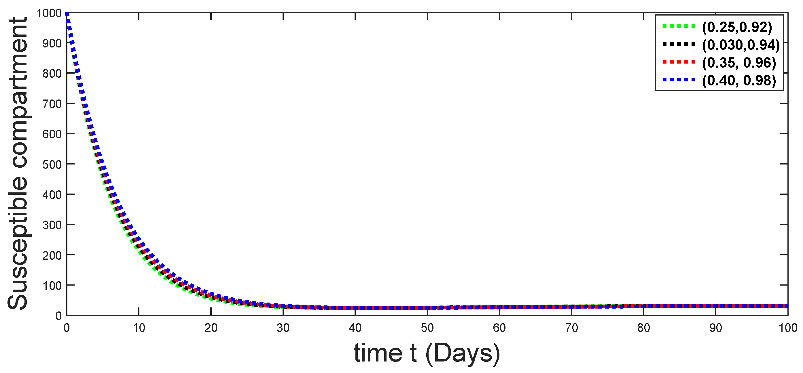
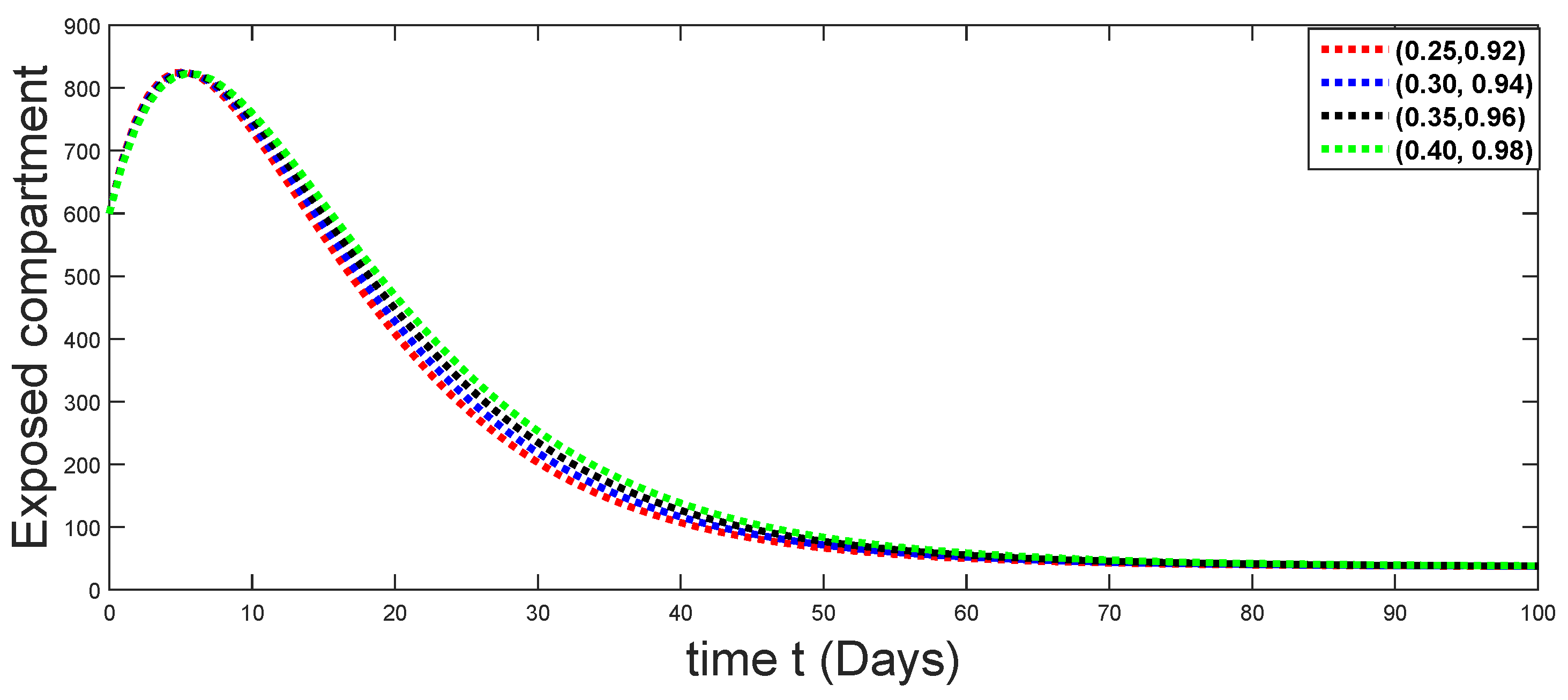
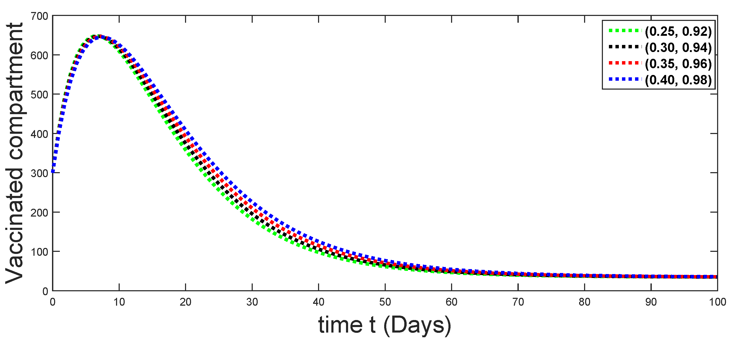
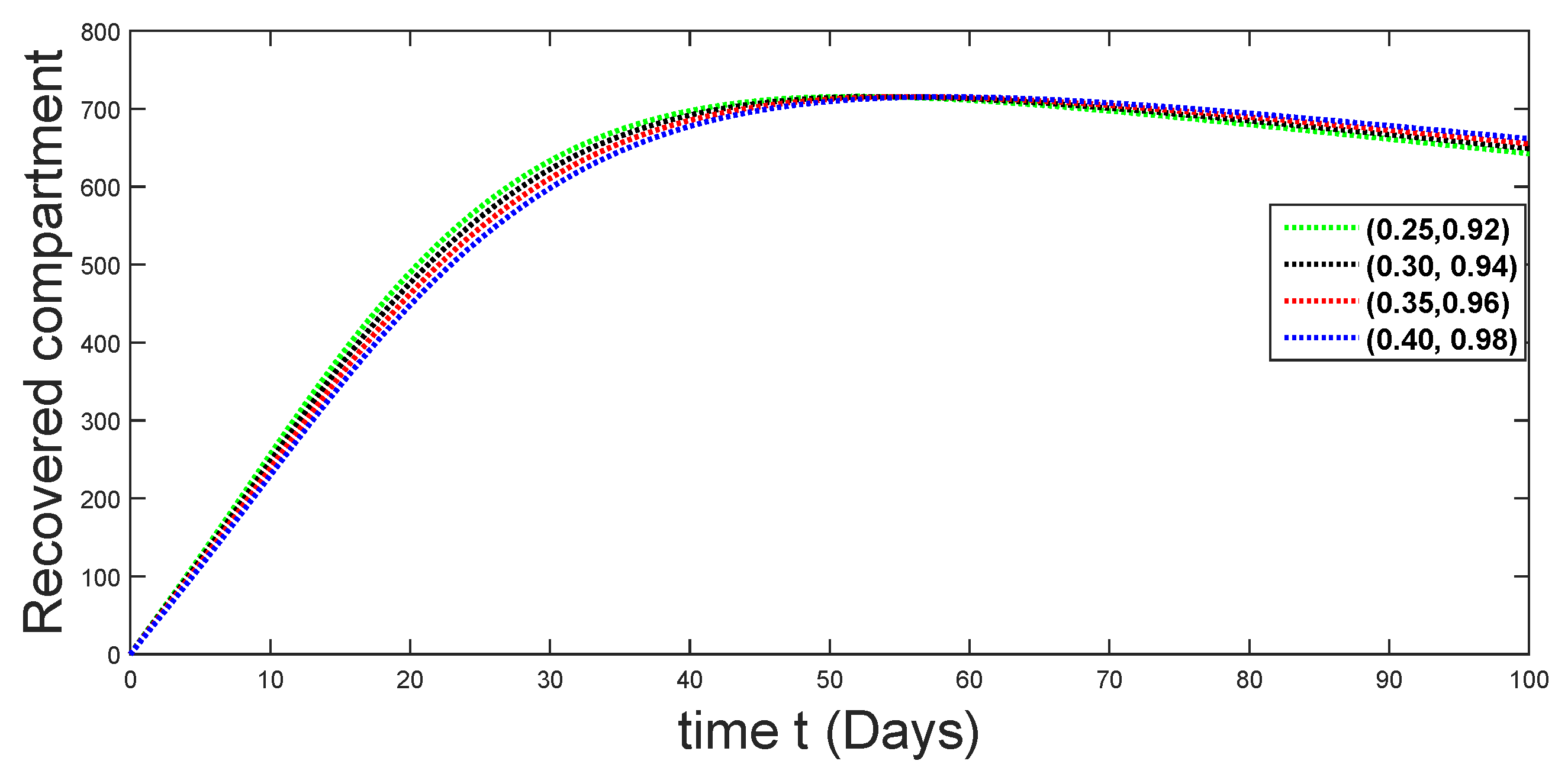
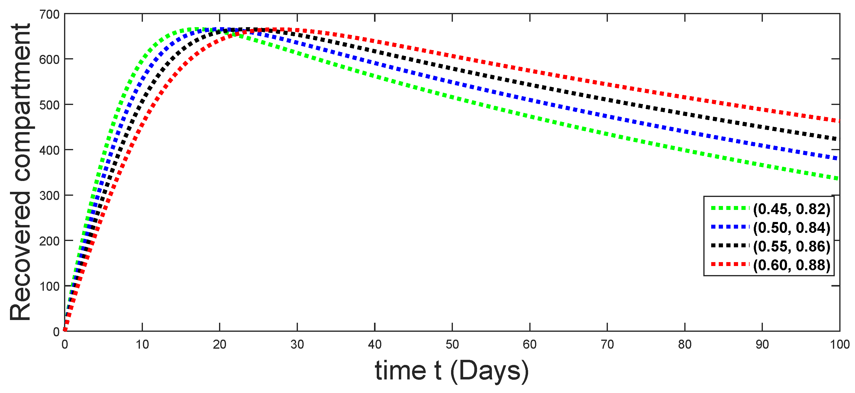
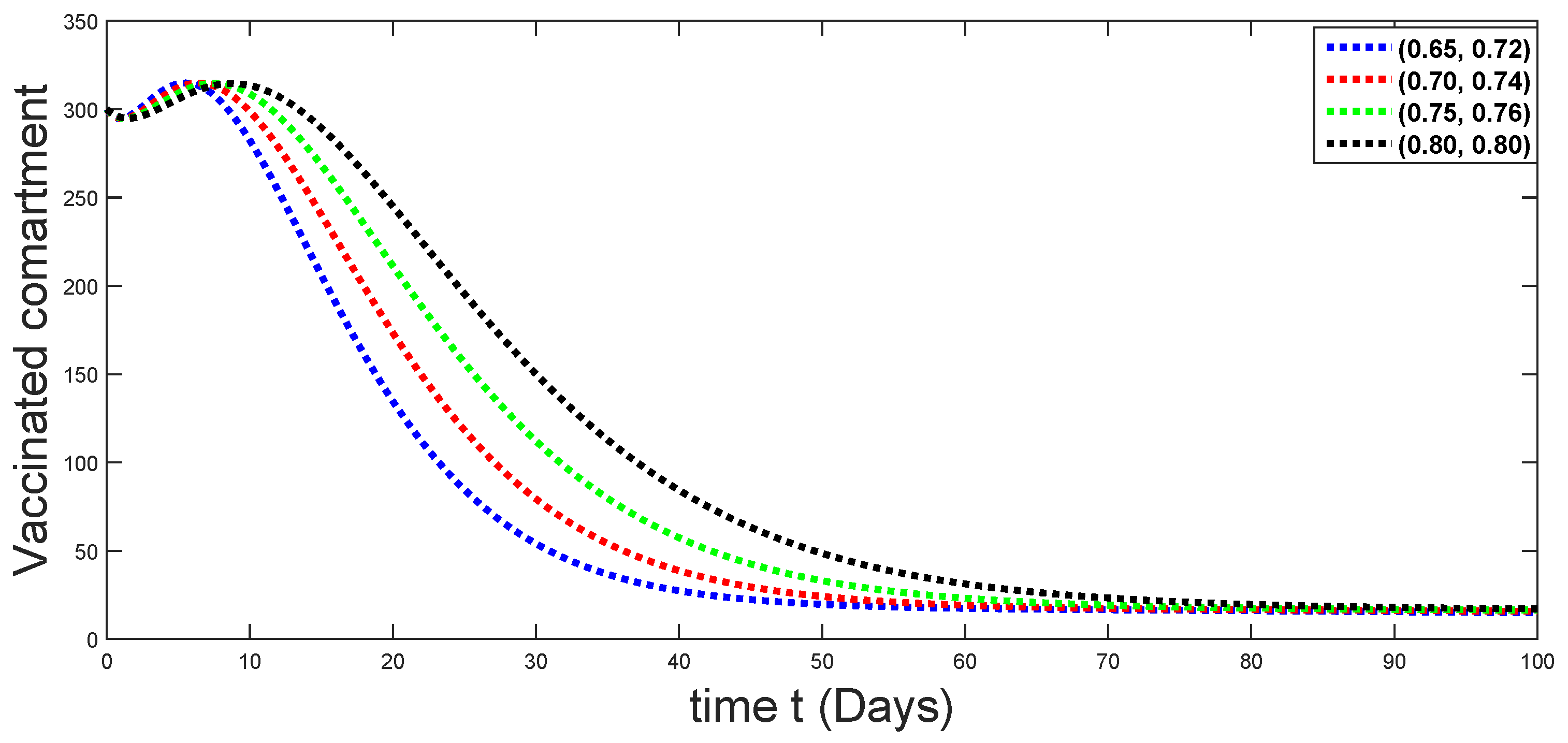
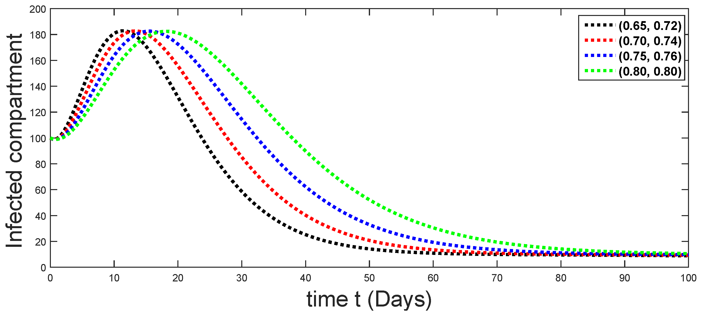
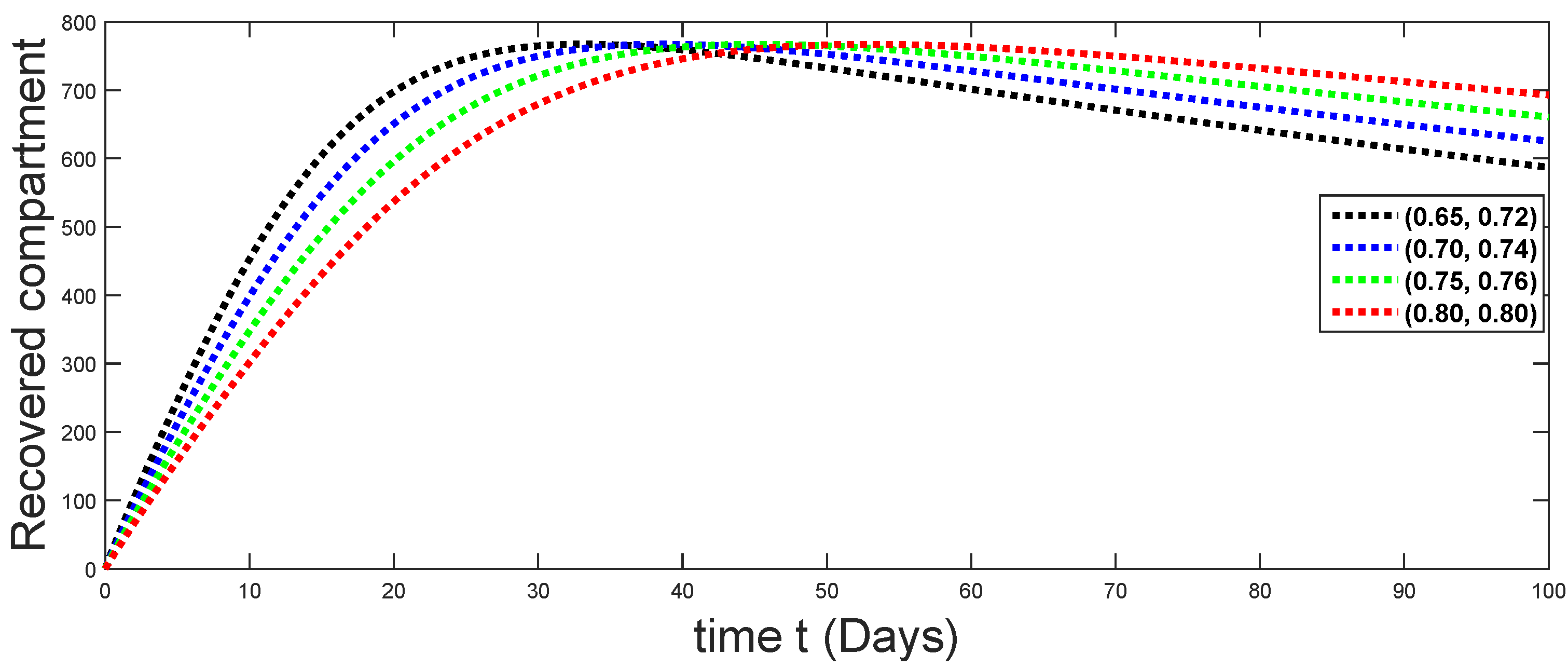
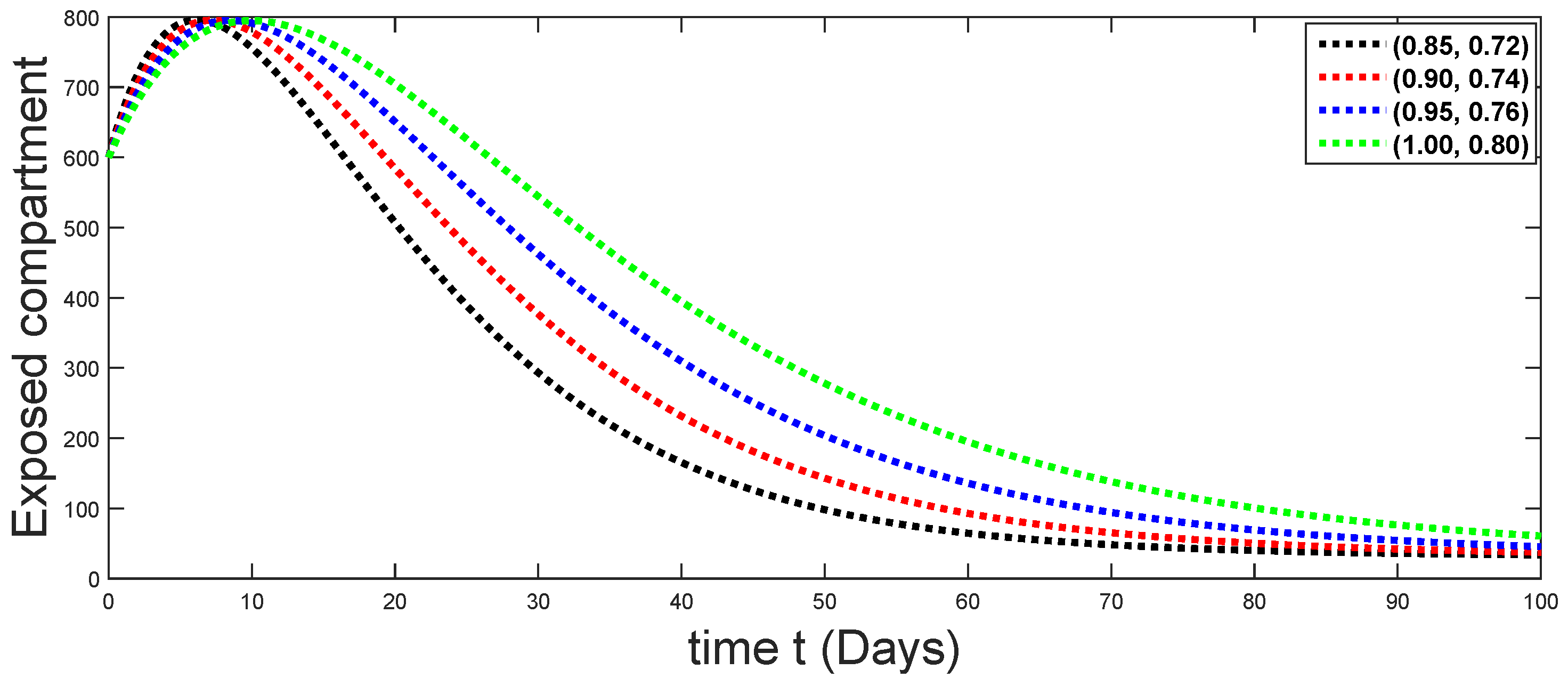
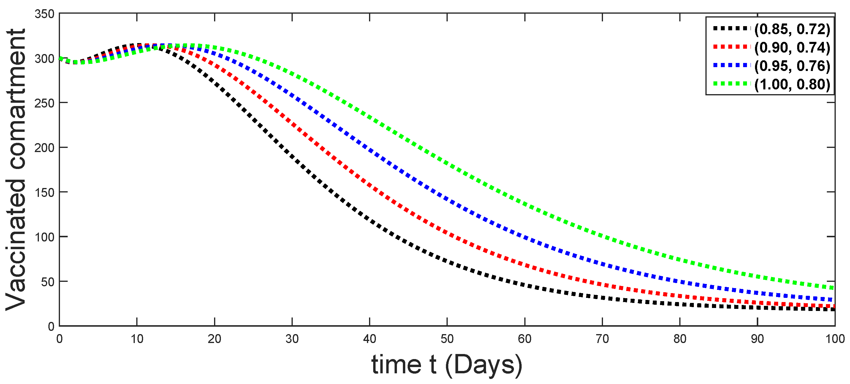
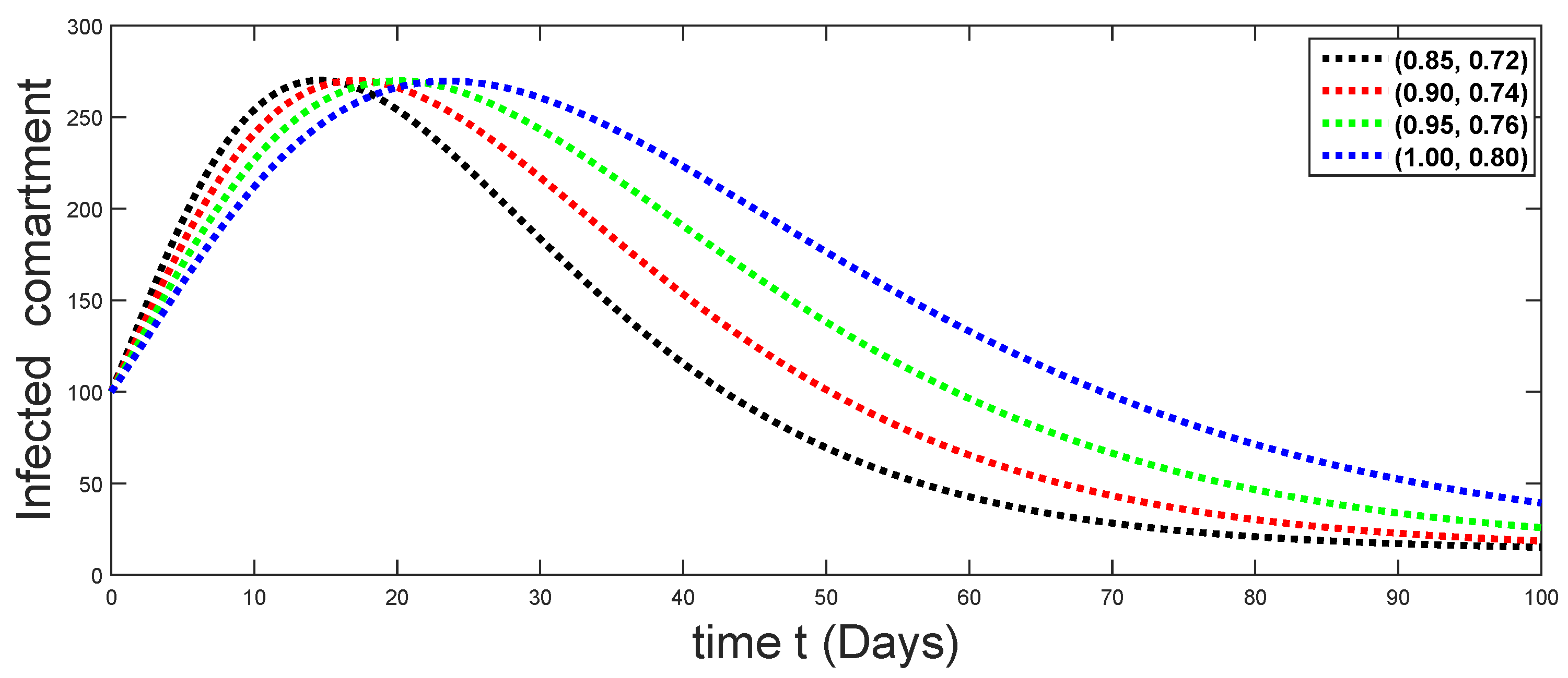
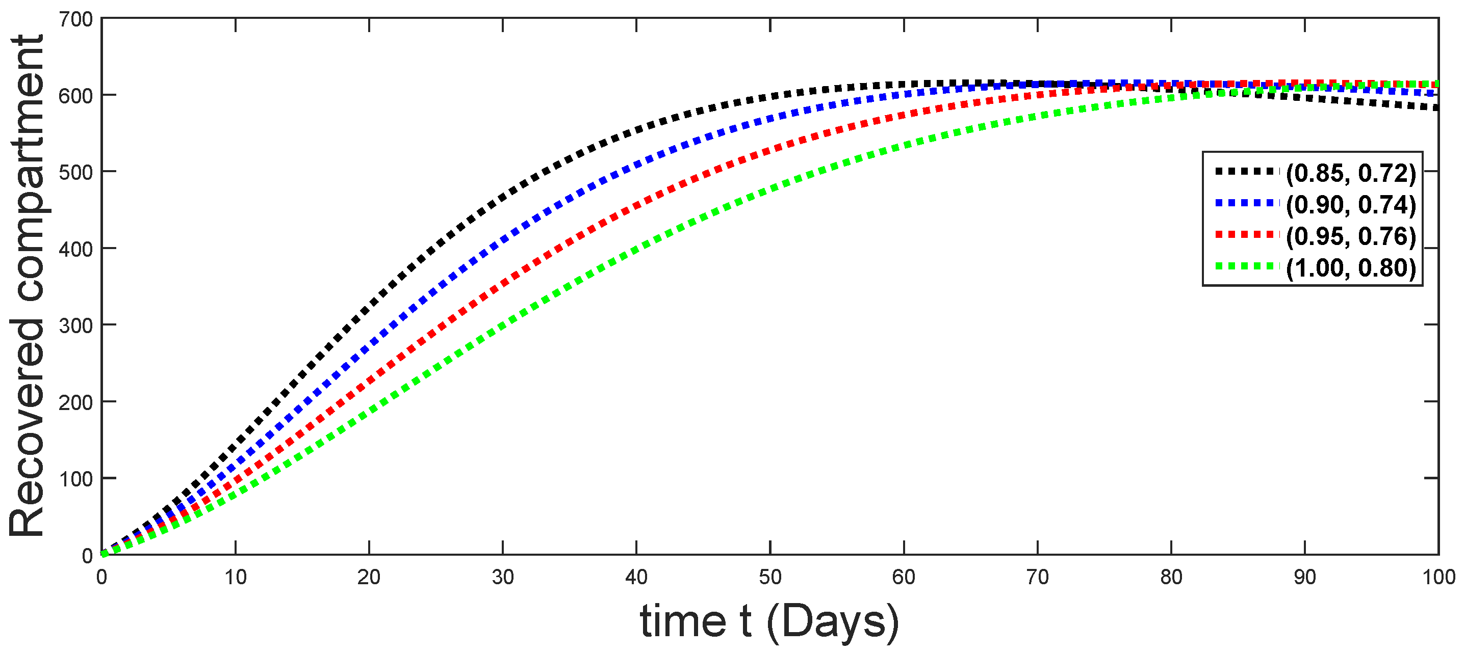
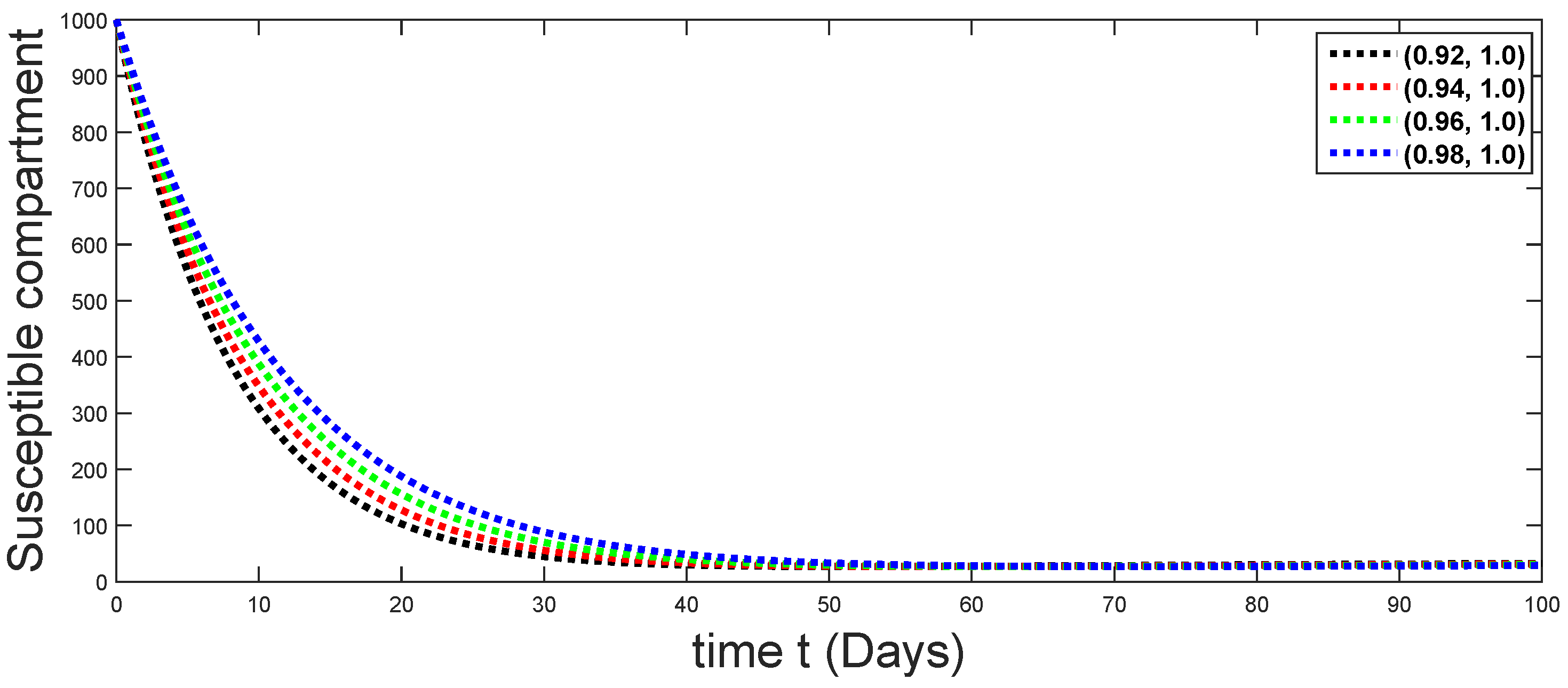
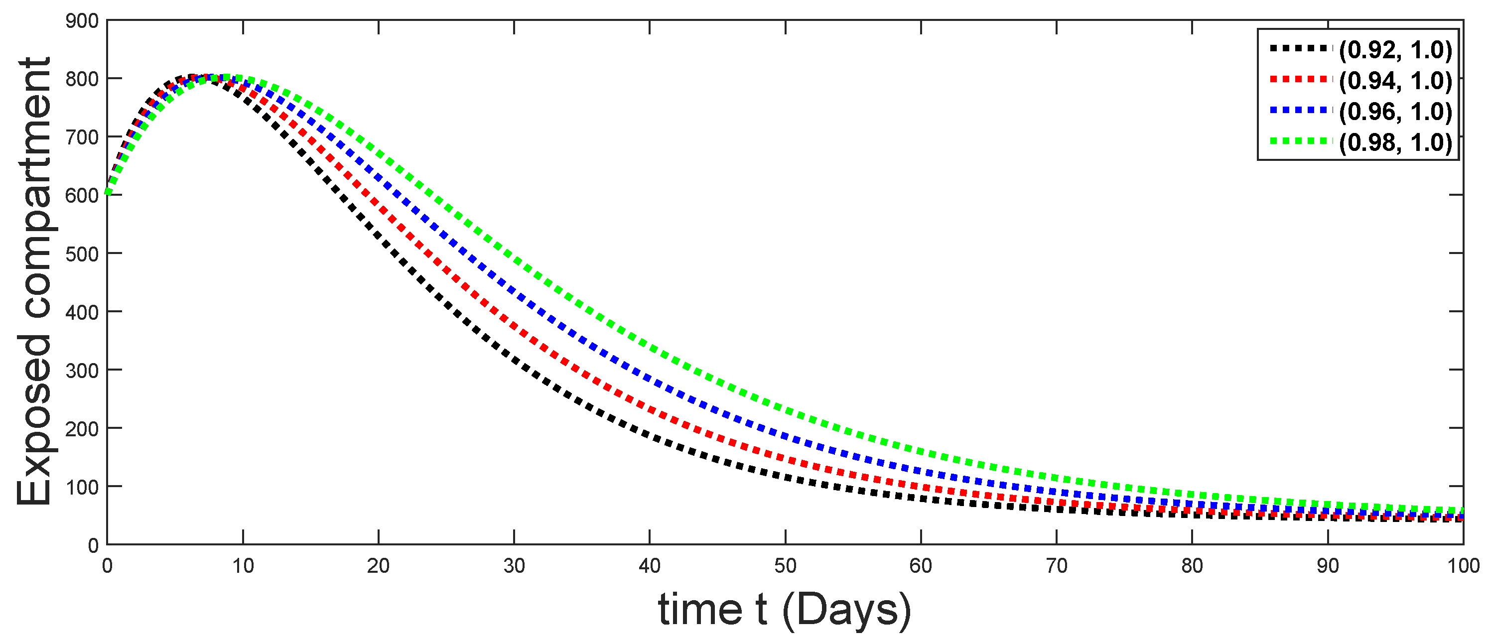
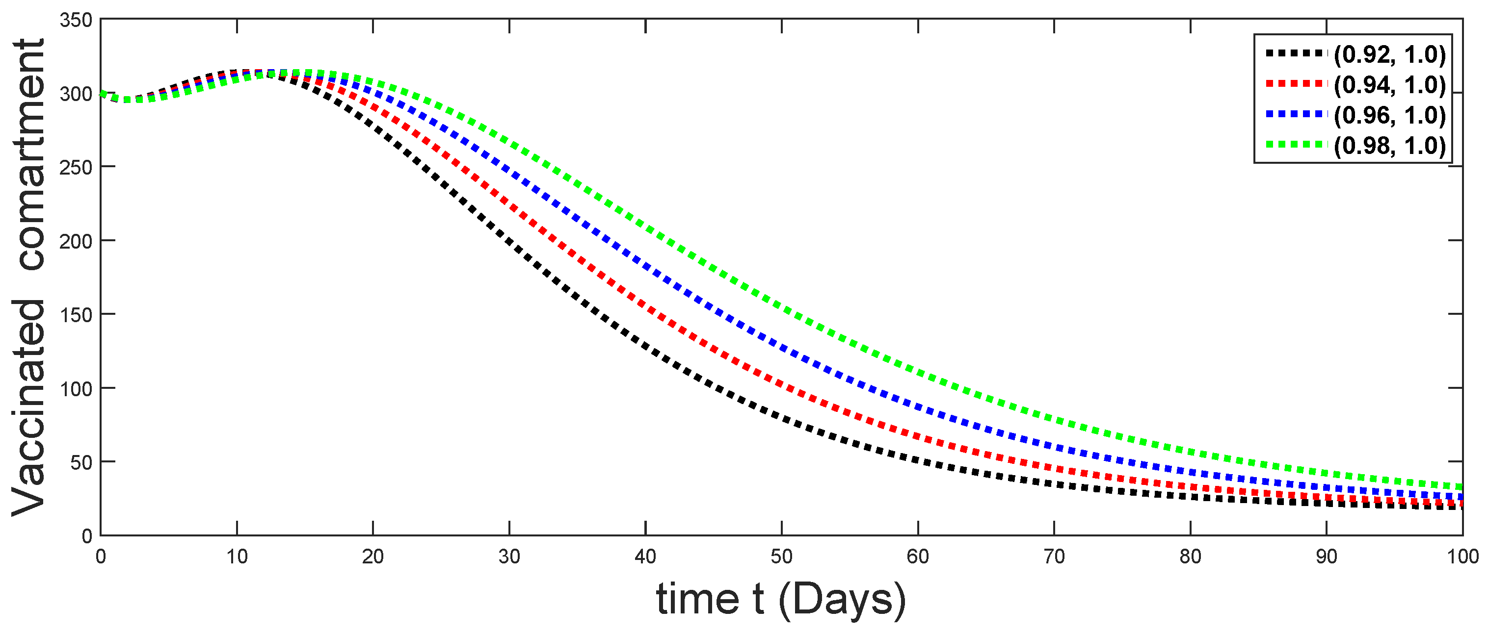
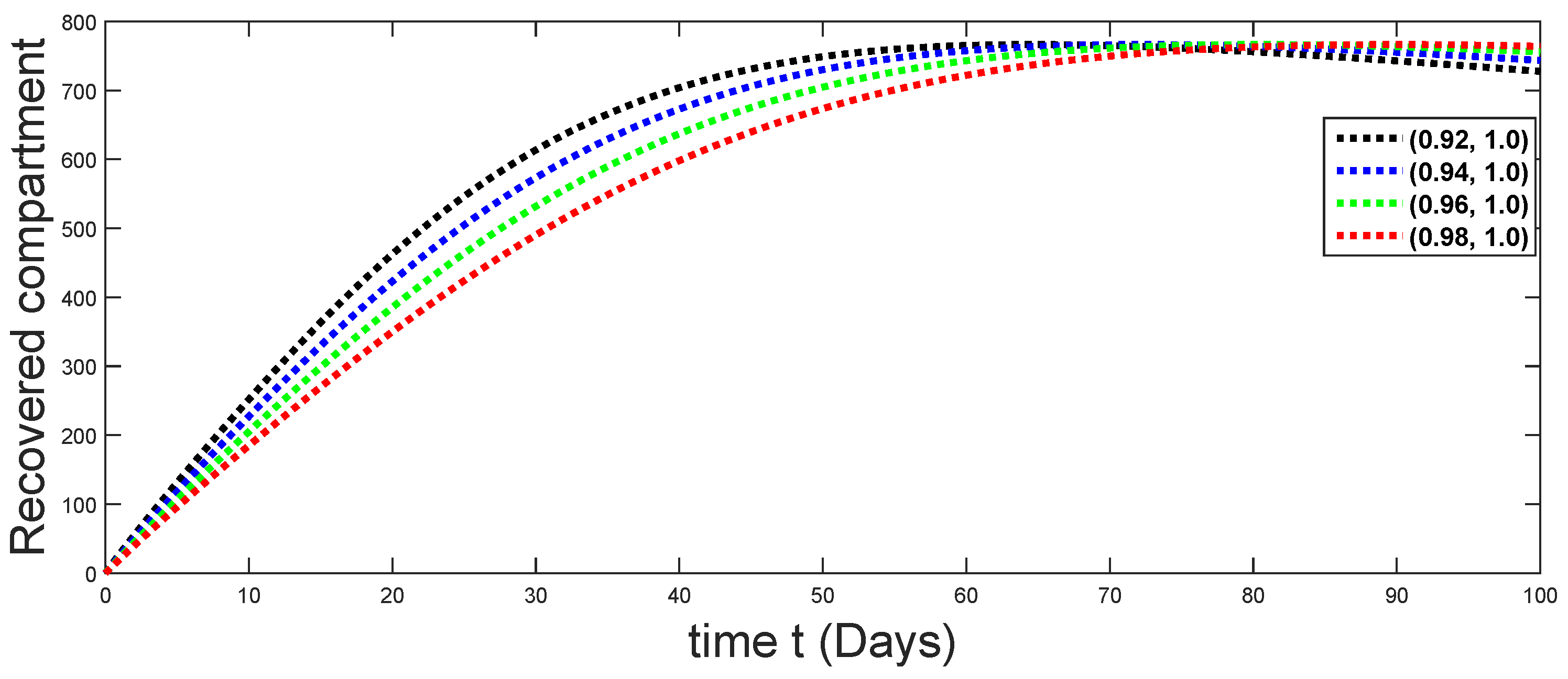
6. Numerical Presentation

Here, we have utilized the aforesaid numerical method to present our results graphically. We have considered the initial values [49] as $(S_0,V_0,E_0,I_0,R_0)=(1000,300,600,100,0)$ and the parameters values as described by Table 1. Here, we use five different sets of fractal fractional order values which have been explained in five different steps as follows:

6.1. When $\xi \in (0.90,0.98],\sigma \in (0,0.40]$

We have used the corresponding values of fractal fractional order to graphically interpret the approximate solution for various classes of the considered model in Figure 3, Figure 4, Figure 5, Figure 6 and Figure 7.

6.2. When $\xi \in (0.80,0.88],\sigma \in (0.40,0.60]$

We have used the corresponding values of fractal fractional order to graphically interpret the approximate solution for various classes of the considered model in Figure 8, Figure 9, Figure 10, Figure 11 and Figure 12.

6.3. When $\xi \in (0.70,0.80],\sigma \in (0.60,0.80]$

We have used the corresponding values of fractals fractional order to graphically interpret the approximate solution for various classes of the considered model in Figure 13, Figure 14, Figure 15, Figure 16 and Figure 17.

6.4. When $\xi \in (0.70,0.80],\sigma \in (0.80,1.00]$

We have used the corresponding values of fractal fractional order to graphically interpret the approximate solution for various classes of the considered model in Figure 18, Figure 19, Figure 20, Figure 21 and Figure 22.

6.5. When $\xi =1.0,\sigma \in (0.90,0.98]$

We have used the corresponding values of fractal fractional order to graphically interpret the approximate solution for various classes of the considered model in Figure 23, Figure 24, Figure 25, Figure 26 and Figure 27.

From Figure 3, Figure 4, Figure 5, Figure 6 and Figure 7, we see that as the population of the susceptible class decreases with different fractal fractional orders values, the number of vaccinated individuals consequently increases for some time, and afterwards it decreases. Also, the number of susceptible individuals decreases due to the fact that they are exposed to infection, and hence infection grows initially. But in the presence of vaccination, the infection goes on to decrease, and hence the population of recovered individuals increases. Here, we should be keep in mind that four different sets of fractal fractional orders have been used to see that effect on the transmission dynamics of fractal fractional orders. In the same way, from Figure 8, Figure 9, Figure 10, Figure 11, Figure 12, Figure 13, Figure 14, Figure 15, Figure 16, Figure 17, Figure 18, Figure 19, Figure 20, Figure 21, Figure 22, Figure 23, Figure 24, Figure 25, Figure 26 and Figure 27, we can observe that the susceptible class grows smaller with time and that various curves start to develop, until it eventually stabilizes. The decay process is faster at lower values of fractal and fractional orders. The vaccination process is grows, then reduces and becomes stable after some time. At the same time, the exposed class population initially increases and then decreases. The infection first increases, but after vaccination and recovery from infection, it continues decreasing. The recovery classes grows smoothly and achieves a stable position. One thing that should be kept in mind is that stability behaviour is asymptotical in all classes. Here, as the fractional order $\sigma \to 1$, the curves are neatly approaching the curve at $\sigma =1$. In the last case, we have considered $\xi =1$; then, the concerned model reduces to a standard fractional order model, for which we have simulated the results at some fractional order values by taking $h=0.01$. The dynamical behaviours are almost same as in the previous cases. Here, we see that as fractals order $\xi \to 1$ and $\sigma \to 1$, the curves in the graphs tend to be close to the solution curves at the integer order of different classes.

7. Concluding Remarks

A dynamical system of eye infectious disease was considered in this research work under fractal and fractional order derivatives. The results obtained by the adopted operators, compared to classical or fractional order derivatives, have plausible effect. The concerned operator has involved the Mittag–Leffler kernel. Sufficient conditions for existence and Hyers–Ulam stability were deduced by using a fixed point approach and nonlinear functional analysis. In addition, the positivity and boundedness conditions were investigated for the solution of the proposed model. In addition, equilibrium points, including disease-free and endemic as well as the basic reproductive number, have been computed. Finally, a sophisticated numerical algorithm based on interpolation was derived. The approximate solutions for different classes, using various values of fractal fractional orders, were presented graphically in five subsections. We have considered several cases to investigate the transmission dynamics of the proposed model against different fractional and fractal orders. The aforesaid orders have a great impact on dynamical behaviour because, at greater fractional order values, by taking $\xi =1$, we see that as $\sigma \to 1$, the dynamics of various compartments coincides with those of integer orders dynamics. Hence, finally, we concluded that understanding the dynamics of eye infectious disease transmission and developing effective tactics to address it in light of fractal and fractional calculus can be facilitated very well by the application of modelling and optimization approaches. The investigated model is a five-compartments model that does not present us with complete, detailed information about the eradication of disease and permanently controlling it. Our formulated model does not contain the control measures of isolation and hygiene compliance. It is necessary to investigate the best control schemes for the direct and indirect transmission dynamics of conjunctivitis. Therefore, to deduce comprehensive details about the control strategies, in the future, optimal control procedures should be incorporated. The disease transmission dynamics under various incidence rates like convex, and nonlinear incidence rate, should be involved to investigate the transmission dynamics. The concerned analysis and results can be extended to a further more generalized model of the spread of conjunctivitis adenovirus disease in the future. The stochastic form of said model can be investigated in the future.

References

1. Center for Disease Control (CDC). Conjunctivitis (Pink Eye). 2022. Available online: https://www.cdc.gov (accessed on 31 December 2023).
2. Fehily, S.R.; Cross, G.B.; Fuller, A.J. Bilateral conjunctivitis in a returned traveller. PLoS Neglected Trop. 2015, 9, e0003351. [Google Scholar] [CrossRef]
3. Elliot, R.H. Conjunctivitis in the tropics. Br. Med. J. 1925, 1, 12–14. [Google Scholar] [CrossRef]
4. Malu, K.N. Allergic conjunctivitis in Jos-Nigeria. Niger. Med. J. J. Niger. Med. Assoc. 2014, 55, 166–170. [Google Scholar] [CrossRef]
5. Kimberlin, D.W. Red Book: 2018–2021 Report of the Committee on Infectious Diseases; American Academy of Pediatrics: Elk Grove Village, IL, USA, 2018; No. Ed. 31. [Google Scholar]
6. Chowell, G.; Shim, E.; Brauer, F.; Diaz-Dueas, P.; Hyman, J.M.; Castillo-Chavez, C. Modelling the transmission dynamics of acute haemorrhagic conjunctivitis: Application to the 2003 outbreak in Mexico. Stat. Med. 2006, 25, 1840–1857. [Google Scholar] [CrossRef]
7. Murray, J.D. Mathematical Biology I; Springer: Berlin, Germany, 2003. [Google Scholar]
8. Ohlsson, F.; Borgqvist, J.; Cvijovic, M. Symmetry structures in dynamic models of biochemical systems. J. R. Soc. Interface 2020, 17, 20200204. [Google Scholar] [CrossRef]
9. Wilson, H.R.; Wilkinson, F. Symmetry perception: A novel approach for biological shapes. Vis. Res. 2002, 42, 589–597. [Google Scholar] [CrossRef]
10. Almeida, R.; Malinowska, A.B.; Monteiro, M.T.T. Fractional differential equations with a Caputo derivative with respect to a kernel function and their applications. Math. Methods Appl. Sci. 2018, 41, 336–352. [Google Scholar] [CrossRef]
11. Das, S.; Pan, I. Fractional Order Signal Processing: Introductory Concepts and Applications; Springer Science & Business Media: Berlin, Germnay, 2011. [Google Scholar]
12. Araz, S.İ. Analysis of a COVID-19 model: Optimal control, stability and simulations. Alex. Eng. J. 2021, 60, 647–658. [Google Scholar] [CrossRef]
13. Awadalla, M.; Yameni, Y. Modeling exponential growth and exponential decay real phenomena by ψ-Caputo fractional derivative. J. Adv. Math. Comput. Sci. 2018, 28, 1–13. [Google Scholar] [CrossRef]
14. Atangana, A.; İğret Araz, S. Mathematical model of COVID-19 spread in Turkey and South Africa: Theory, methods, and applications. Adv. Differ. Equ. 2020, 2020, 659. [Google Scholar] [CrossRef]
15. Ahmed, S.; Ahmed, A.; Mansoor, I.; Junejo, F.; Saeed, A. Output feedback adaptive fractional-order super-twisting sliding mode control of robotic manipulator. Iran. J. Sci. Technol. Trans. Electr. Eng. 2021, 45, 335–347. [Google Scholar] [CrossRef]
16. Shah, K.; Jarad, F.; Abdeljawad, T. On a nonlinear fractional order model of dengue fever disease under Caputo-Fabrizio derivative. Alex. Eng. J. 2020, 59, 2305–2313. [Google Scholar] [CrossRef]
17. Ahmed, S.; Wang, H.; Aslam, M.S.; Ghous, I.; Qaisar, I. Robust adaptive control of robotic manipulator with input time-varying delay. Int. J. Control Autom. Syst. 2019, 17, 2193–2202. [Google Scholar] [CrossRef]
18. Shaikh, A.; Nisar, K.S.; Jadhav, V.; Elagan, S.K.; Zakarya, M. Dynamical behaviour of HIV/AIDS model using fractional derivative with Mittag-Leffler kernel. Alex. Eng. J. 2022, 61, 2601–2610. [Google Scholar] [CrossRef]
19. Peter, O.J.; Shaikh, A.S.; Ibrahim, M.O.; Nisar, K.S.; Baleanu, D.; Khan, I.; Abioye, A.I. Analysis and dynamics of fractional order mathematical model of COVID-19 in Nigeria using atangana-baleanu operator. Comput. Mater. Contin. 2021, 66, 1823–1848. [Google Scholar] [CrossRef]
20. Shaikh, A.S.; Shaikh, I.N.; Nisar, K.S. A mathematical model of COVID-19 using fractional derivative: Outbreak in India with dynamics of transmission and control. Adv. Differ. Equ. 2020, 2020, 373. [Google Scholar] [CrossRef] [PubMed]
21. Teodoro, G.S.; Machado, J.T.; De Oliveira, E.C. A review of definitions of fractional derivatives and other operators. J. Comput. Phys. 2019, 388, 195–208. [Google Scholar] [CrossRef]
22. Khalil, R.; Al Horani, M.; Yousef, A.; Sababheh, M. A new definition of fractional derivative. J. Comput. Appl. Math. 2014, 264, 65–70. [Google Scholar] [CrossRef]
23. Hilfer, R. (Ed.) Applications of Fractional Calculus in Physics; World Scientific: Singapore, 2000. [Google Scholar]
24. Kilbas, A.A. Hadamard-type fractional calculus. J. Korean Math. Soc. 2001, 38, 1191–1204. [Google Scholar]
25. Zhang, T.; Li, Y. Global exponential stability of discrete-time almost automorphic Caputo-Fabrizio BAM fuzzy neural networks via exponential Euler technique. Knowl.-Based Syst. 2022, 246, 108675. [Google Scholar] [CrossRef]
26. Khan, M.; Ahmad, Z.; Ali, F.; Khan, N.; Khan, I.; Nisar, K.S. Dynamics of two-step reversible enzymatic reaction under fractional derivative with Mittag-Leffler Kernel. PLoS ONE 2023, 18, e0277806. [Google Scholar] [CrossRef]
27. Caputo, M.; Fabrizio, M. Applications of new time and spatial fractional derivatives with exponential kernels. Prog. Fract. Differ. Appl. 2016, 2, 1–11. [Google Scholar] [CrossRef]
28. Caputo, M.; Fabrizio, M. A new definition of fractional derivative without singular kernel. Progr. Fract. Differ. Appl. 2015, 1, 73–85. [Google Scholar]
29. Losada, J.; Nieto, J.J. Properties of a new fractional derivative without singular kernel. Progr. Fract. Differ. Appl. 2015, 1, 87–92. [Google Scholar]
30. Gul, R.; Sarwar, M.; Shah, K.; Abdeljawad, T.; Jarad, F. Qualitative analysis of implicit Dirichlet boundary value problem for Caputo-Fabrizio fractional differential equations. J. Funct. Spaces 2020, 2020, 4714032. [Google Scholar] [CrossRef]
31. Atangana, A.; Baleanu, D. New fractional derivatives with non-local and non-singular kernel: Theory and application to heat transfer model. Therm. Sci. 2016, 20, 763–769. [Google Scholar] [CrossRef]
32. Xu, C.; Liu, Z.; Pang, Y.; Saifullah, S.; Inc, M. Oscillatory, crossover behavior and chaos analysis of HIV-1 infection model using piece-wise Atangana–Baleanu fractional operator: Real data approach. Chaos Solitons Fractals 2022, 164, 112662. [Google Scholar] [CrossRef]
33. Saifullah, S.; Ali, A.; Irfan, M.; Shah, K. Time-fractional Klein–Gordon equation with solitary/shock waves solutions. Math. Probl. Eng. 2021, 2021, 6858592. [Google Scholar] [CrossRef]
34. Alomari, A.K.; Abdeljawad, T.; Baleanu, D.; Saad, K.M.; Al-Mdallal, Q.M. Numerical solutions of fractional parabolic equations with generalized Mittag-Leffler kernels. Numer. Methods Partial. Differ. Equ. 2024, 40, e22699. [Google Scholar] [CrossRef]
35. Saad Alshehry, A.; Imran, M.; Shah, R.; Weera, W. Fractional-View Analysis of Fokker-Planck equations by ZZ Transform with Mittag-Leffler Kernel. Symmetry 2022, 14, 1513. [Google Scholar] [CrossRef]
36. Atangana, A. Fractal-fractional differentiation and integration: Connecting fractal calculus and fractional calculus to predict complex system. Chaos Solitons Fractals 2017, 102, 396–406. [Google Scholar] [CrossRef]
37. He, J.H. Fractal calculus and its geometrical explanation. Results Phys. 2018, 10, 272–276. [Google Scholar] [CrossRef]
38. Hu, Y.; He, J.H. On fractal space-time and fractional calculus. Therm. Sci. 2016, 20, 773–777. [Google Scholar] [CrossRef]
39. Qureshi, S.; Atangana, A. Fractal-fractional differentiation for the modeling and mathematical analysis of nonlinear diarrhea transmission dynamics under the use of real data. Chaos Solitons Fractals 2020, 136, 109812. [Google Scholar] [CrossRef]
40. Srivastava, H.M.; Saad, K.M. Numerical simulation of the fractal-fractional Ebola virus. Fractal Fract. 2020, 4, 49. [Google Scholar] [CrossRef]
41. Xiao, B.; Huang, Q.; Chen, H.; Chen, X.; Long, G. A fractal model for capillary flow through a single tortuous capillary with roughened surfaces in fibrous porous media. Fractals 2021, 29, 2150017. [Google Scholar] [CrossRef]
42. Liang, M.; Liu, Y.; Xiao, B.; Yang, S.; Wang, Z.; Han, H. An analytical model for the transverse permeability of gas diffusion layer with electrical double layer effects in proton exchange membrane fuel cells. Int. J. Hydrogen Energy 2018, 43, 17880–17888. [Google Scholar] [CrossRef]
43. Yu, X.; Xu, H.; Zhai, C.; Regenauer-Lieb, K.; Sang, S.; Sun, Y.; Jing, Y. Characterization of water migration behavior during spontaneous imbibition in coal: From the perspective of fractal theory and NMR. Fuel 2024, 355, 129499. [Google Scholar] [CrossRef]
44. Ahmad, I.; Ahmad, N.; Shah, K.; Abdeljawad, T. Some appropriate results for the existence theory and numerical solutions of fractals-fractional order malaria disease mathematical model. Results Control. Optim. 2024, 14, 100386. [Google Scholar] [CrossRef]
45. Abro, K.A. Role of fractal–fractional derivative on ferromagnetic fluid via fractal Laplace transform: A first problem via fractal-fractional differential operator. Eur. J. Mech.-B/Fluids 2021, 85, 76–81. [Google Scholar] [CrossRef]
46. Atangana, A.; Goufo, E.F.D. Cauchy problems with fractal-fractional operators and applications to groundwater dynamics. Fractals 2020, 28, 2040043. [Google Scholar] [CrossRef]
47. Atangana, A.; Qureshi, S. Modeling attractors of chaotic dynamical systems with fractal–fractional operators. Chaos Solitons Fractals 2019, 123, 320–337. [Google Scholar] [CrossRef]
48. Sangsawang, S.; Tanutpanit, T.; Mumtong, W.; Pongsumpun, P. Local stability analysis of mathematical model for hemorrhagic conjunctivitis disease. Curr. Appl. Sci. Technol. 2012, 12, 189–197. [Google Scholar]
49. Javed, F.; Ahmad, A.; Ali, A.H.; Hincal, E.; Amjad, A. Investigation of conjunctivitis adenovirus spread in human eyes by using bifurcation tool and numerical treatment approach. Phys. Scr. 2024, 99, 085253. [Google Scholar] [CrossRef]
50. Fatunla, S.O. Numerical Methods for Initial Value Problems in Ordinary Differential Equations; Academic Press: New York, NY, USA, 2014. [Google Scholar]
51. Khan, M.A.; Atangana, A. Numerical Methods for Fractal-Fractional Differential Equations and Engineering: Simulations and Modeling; CRC Press: New York, NY, USA, 2023. [Google Scholar]
52. Van den Driessche, P.; Watmough, J. Reproduction numbers and sub-threshold endemic equilibria for compartmental models of disease transmission. Math. Biosci. 2002, 180, 29–48. [Google Scholar] [CrossRef]
53. Van den Driessche, P.; Watmough, J. Further notes on the basic reproduction number. Math. Epidemiol. 2008, 2008, 159–178. [Google Scholar]
54. DeJesus, E.X.; Kaufman, C. Routh-Hurwitz criterion in the examination of eigenvalues of a system of nonlinear ordinary differential equations. Phys. Rev. A 1987, 35, 5288. [Google Scholar] [CrossRef] [PubMed]
55. Castillo-Chavez, C.; Blower, S.; van den Driessche, P.; Kirschner, D.; Yakubu, A.A. (Eds.) Mathematical Approaches for Emerging and Reemerging Infectious Diseases: Models, Methods, and Theory; Springer Science & Business Media: New York, NY, USA, 2002; Volume 126. [Google Scholar]
56. Arriola, L.M.; Hyman, J.M. Being sensitive to uncertainty. Comput. Sci. Eng. 2007, 9, 10–20. [Google Scholar] [CrossRef]
57. Khan, A.; Zarin, R.; Hussain, G.; Usman, A.H.; Humphries, U.W.; Gomez-Aguilar, J.F. Modeling and sensitivity analysis of HBV epidemic model with convex incidence rate. Results Phys. 2021, 22, 103836. [Google Scholar] [CrossRef]
58. Hyers, D.H. On the stability of the linear functional equation. Proc. Natl. Acad. Sci. USA 1941, 27, 222–224. [Google Scholar] [CrossRef]
59. Rassias, T.M. On the stability of the linear mapping in Banach spaces. Proc. Natl. Acad. Sci. USA 1978, 72, 297–300. [Google Scholar] [CrossRef]
60. Sher, M.; Shah, K.; Rassias, J. On qualitative theory of fractional order delay evolution equation via the prior estimate method. Math. Methods Appl. Sci. 2020, 43, 6464–6475. [Google Scholar] [CrossRef]
61. Yanagiwara, H.I.R.O.K.I. On the Stability of a Multistep Method. In Proceedings of the Sixth International Colloquim on Differential Equations, Plovdiv, Bulgaria, 18–23 August 1995; pp. 369–376. [Google Scholar]
62. Sehnalová, P. Stability and convergence of numerical computations. Inf. Sci. Technol. Bull. Acm Slovak. 2011, 3, 26–35. [Google Scholar]
63. Li, C.; Tao, C. On the fractional Adams method. Comput. Math. Appl. 2009, 58, 1573–1588. [Google Scholar] [CrossRef]
Figure 1. Schematic diagram of model (3).
Symmetry 16 01284 g001
Figure 2. (a) Graphical presentation of R 0 using α , μ n . (b) Graphical presentation of R 0 using β , λ . (c) Graphical presentation of R 0 using γ , μ . (d) Graphical presentation of R 0 using Λ , μ .
Symmetry 16 01284 g002
Figure 3. Dynamical behaviors of susceptible compartments against using different fractal fractional orders in ( 0 , 0.30 ] .
Symmetry 16 01284 g003
Figure 4. Dynamical behaviors of exposed compartments against using different fractal fractional orders in ( 0 , 0.30 ] .
Symmetry 16 01284 g004
Figure 5. Dynamical behaviors of vaccinated compartments against using different fractal fractional orders in ( 0 , 0.30 ] .
Symmetry 16 01284 g005
Figure 6. Dynamical behaviors of infected compartments against using different fractal fractional orders in ( 0 , 0.30 ] .
Symmetry 16 01284 g006
Figure 7. Dynamical behaviors of recovered compartments against using different fractal fractional orders in ( 0 , 0.30 ] .
Symmetry 16 01284 g007
Figure 8. Dynamical behaviors of susceptible compartments against using different fractal fractional orders in ( 0.40 , 0.60 ] .
Symmetry 16 01284 g008
Figure 9. Dynamical behaviors of exposed compartments against using different fractal fractional orders in ( 0.40 , 0.60 ] .
Symmetry 16 01284 g009
Figure 10. Dynamical behaviors of vaccinated compartments against using different fractal fractional orders in ( 0.40 , 0.60 ] .
Symmetry 16 01284 g010
Figure 11. Dynamical behaviors of infected compartments against using different fractal fractional orders in ( 0.40 , 0.60 ] .
Symmetry 16 01284 g011
Figure 12. Dynamical behaviors of recovered compartments against using different fractal fractional orders in ( 0.40 , 0.60 ] .
Symmetry 16 01284 g012
Figure 13. Dynamical behaviors of susceptible compartments against using different fractal fractional orders in ( 0.60 , 0.80 ] .
Symmetry 16 01284 g013
Figure 14. Dynamical behaviors of exposed compartments against using different fractal fractional orders in ( 0.60 , 0.80 ] .
Symmetry 16 01284 g014
Figure 15. Dynamical behaviors of vaccinated compartments against using different fractal fractional orders in ( 0.60 , 0.80 ] .
Symmetry 16 01284 g015
Figure 16. Dynamical behaviors of infected compartments against using different fractal fractional orders in ( 0.60 , 0.80 ] .
Symmetry 16 01284 g016
Figure 17. Dynamical behaviors of recovered compartments against using different fractal fractional orders in ( 0.60 , 0.80 ] .
Symmetry 16 01284 g017
Figure 18. Dynamical behaviors of susceptible compartments against using different fractal fractional orders in ( 0.80 , 1.00 ] .
Symmetry 16 01284 g018
Figure 19. Dynamical behaviors of exposed compartments against using different fractal fractional orders in ( 0.80 , 1.00 ] .
Symmetry 16 01284 g019
Figure 20. Dynamical behaviors of vaccinated compartments against using different fractal fractional orders in ( 0.80 , 1.00 ] .
Symmetry 16 01284 g020
Figure 21. Dynamical behaviors of infected compartments against using different fractal fractional orders in ( 0.80 , 1.00 ] .
Symmetry 16 01284 g021
Figure 22. Dynamical behaviors of recovered compartments against using different fractal fractional orders in ( 0.80 , 1.00 ] .
Symmetry 16 01284 g022
Figure 23. Dynamical behaviors of susceptible compartments against using different fractal fractional orders in ( 0.90 , 0.98 ] .
Symmetry 16 01284 g023
Figure 24. Dynamical behaviors of exposed compartments against using different fractal fractional orders in ( 0.90 , 0.98 ] .
Symmetry 16 01284 g024
Figure 25. Dynamical behaviors of vaccinated compartments against using different fractal fractional orders in ( 0.90 , 0.98 ] .
Symmetry 16 01284 g025
Figure 26. Dynamical behaviors of infected compartments against using different fractal fractional orders in ( 0.90 , 0.98 ] .
Symmetry 16 01284 g026
Figure 27. Dynamical behaviors of recovered compartments against using different fractal fractional orders in ( 0.90 , 0.98 ] .
Symmetry 16 01284 g027