New Processing Technique of Jacobian Elliptic Equation and Its Application to the (3+1)-Dimensional Modified Korteweg de Vries–Zakharov–Kuznetsov Equation

Abstract

This article introduces two kinds of processing techniques to solve Jacobian elliptic equations and obtain rich periodic wave solutions. Then, the equation was used as an auxiliary equation to solve the (3+1)-dimensional modified Korteweg de Vries–Zakharov–Kuznetsov (mKDV-ZK) equation. Combined with the mapping method, a large number of new types of exact periodic wave solutions were obtained, many of which were rarely found in previous research. Numerical simulations have demonstrated the evolution of various periodic waves in (3+1)-dimensional mKDV-ZK. The solutions and wave phenomena obtained in this article will help expand our understanding of the equation.

1. Introduction

The widespread nonlinear problems in the fields of natural and social sciences are receiving increasing attention, and many nonlinear discrimination problems can be described by using the nonlinear evolution equations (NLEEs). In modern physics and engineering, many famous NLEEs have been developed to explain the dynamics of nonlinear waves [1,2,3,4,5,6]. Therefore, how to obtain their exact solutions is very important for the research of related nonlinear problems, and this has always been a core issue in mathematics and physics [7,8,9,10,11,12]. In recent years, great progress has been made, and many powerful and effective methods have been developed to obtain the exact solution of NLEEs [13,14,15,16,17,18,19,20,21,22,23,24,25,26,27,28,29]. In this article, we consider exploring the new exact solutions for the following (3+1)-dimensional mKDV-ZK equation [30].

$$u_t+\alpha u^2{u}_x+\beta {{(u}_{xx}+u_{yy}+u_{zz})}_x=0.$$

(1)

The equation simulates the propagation of nonlinear waves in fluid dynamics, nonlinear optics, and quantum mechanics. The physical characteristics such as wave propagation speed and waveform changes obtained from the wave phenomena of Equation (1) have important practical application value for understanding the wave behavior of shallow water waves, long gravity waves, etc., in fluids, the propagation of optical pulses under dispersion and nonlinear effects in fiber optic communication and optical waveguides, wave behavior and particle interactions in quantum systems, predicting the propagation laws of these nonlinear waves, and optimizing their dynamic design. With the development of the solving process of NLEEs, many methods have been used to solve the (3+1)-dimensional mKDV-ZK equation [30,31,32], and a large number of exact solutions have been obtained. Although these methods are effective in solving the (3+1)-dimensional mKDV-ZK equation, there are still some new methods and new solutions to be explored. The main purpose of this article is to develop two new kinds of function transformations for the Jacobian elliptic equation to construct abundant periodic wave solutions of (3+1)-dimensional mKDV-ZK. Because of these new transformations, the large number of solutions obtained are new solutions that have not been discovered in previous research.

The following is the structure of this article: Section 2 introduces how to construct exact solutions to the Jacobian elliptic equation using two processing techniques. Section 3 expounds on how to apply this method to deal with the (3+1)-dimensional mKDV-ZK equation and obtain a large number of new periodic wave solutions. Section 4 presents a demonstration of a set of solutions and provides intuitive images of nonlinear wave evolution. Finally, we present the discussion and conclusion of this article.

2. Method

Equation (1) is assumed to have a traveling wave solution by taking

$$u\left(x,y,z,t\right)=u(\xi ),\xi =x+y+z-\omega t,$$

(2)

where ω is a wave parameter to be determined. Substituting Equation (2) into Equation (1), integrating it, and then making the integral constant zero, we have

$$-\omega u+{\displaystyle \frac{1}{3}}\alpha u^3+u^{″}=0,$$

(3)

where u′ means du/dξ. Suppose Equation (3) has the following formal solution:

$$u\left(\xi \right)={\sum }_{i=0}^n{a}_i{f}^i\left(\sigma \xi \right)+{\sum }_{i=1}^n{b}_i{f}^{-i}\left(\sigma \xi \right)+{\sum }_{i=2}^n{c}_i{f}^{i-2}\left(\sigma \xi \right)f^{\prime }\left(\sigma \xi \right)+{\sum }_{i=1}^n{d}_i{f}^{-i}\left(\sigma \xi \right)f^{\prime }\left(\sigma \xi \right)$$

(4)

where $\sigma$, a_i, b_i, c_i, and d_i are constants determined later. The positive integer n in Equation (4) can be determined by the homogeneous balance method, which shows that n = 1. Therefore, the solutions of Equation (3) can be written as

$$u\left(\xi \right)=a_0{+a}_{1}f\left(\sigma \xi \right){+b}_1{\displaystyle \frac{1}{f\left(\sigma \xi \right)}}{+d}_1{\displaystyle \frac{f^{\prime }\left(\sigma \xi \right)}{f\left(\sigma \xi \right)}},$$

(5)

where f (ξ) represents the solutions of the following equation:

$${\left[f^{\prime }\left(\xi \right)\right]}^2=p_1{f}^4\left(\xi \right)+q_1{f}^2\left(\xi \right)+r_1,$$

(6)

where p₁, q₁, and r₁ are parameters to be determined. The following function transformation is introduced:

$$f(\xi )={\displaystyle \frac{g\left(\xi \right)}{a_0{g}^2\left(\xi \right)+a_1{g}^{\prime }\left(\xi \right)+a_2}},$$

(7)

where g(ξ) represents the solutions of the following equation:

$${\left[g^{\prime }\left(\xi \right)\right]}^2=p_2{g}^4\left(\xi \right)+q_2{g}^2\left(\xi \right)+r_2,$$

(8)

• where p₂, q₂, and r₂ are parameters of the Jacobian elliptic function. Equation (8) is widely used in the process of solving NLEEs due to its symmetry, constructability, and diversity of solutions [21,22,26]. By selecting different p₂, q₂, and r₂, the mapping of Jacobian elliptic function solutions for Equation (8) is shown in Table 1. It should be pointed out that in the first column of the table, $\mathrm{s}\mathrm{n}(\mathsf{\xi }),\mathrm{c}\mathrm{d}(\mathsf{\xi })=\mathrm{c}\mathrm{n}(\mathsf{\xi })/\mathrm{d}\mathrm{n}(\mathsf{\xi })$ mean $g\left(\xi \right)=sn(\xi )$, and $g(\xi )=cd(\xi )=cn(\xi )/dn(\xi )$.

Table 1. Jacobian elliptic function solutions for Equation (8).

$g\left(\xi \right)$	$p_2$	$q_2$	$r_2$
$sn(\xi ),cd(\xi )=cn(\xi )/dn(\xi )$	$m^2$	$-(1+m^2)$	$1$
$cn(\xi )$	${-m}^2$	$-1+2m^2$	$1-m^2$
$dn(\xi )$	$-1$	$2-m^2$	$-1+m^2$
$ns(\xi )={\displaystyle \frac{1}{sn(\xi )}},$ $dc(\xi )=dn(\xi )/cn(\xi )$	$1$	$-(1+m^2)$	$m^2$
$nc(\xi )=1/cn(\xi )$	$1-m^2$	$-1+2m^2$	${-m}^2$
$nd(\xi )=1/dn(\xi )$	$-1+m^2$	$2-m^2$	$-1$
$cs(\xi )=cn(\xi )/sn(\xi )$	$1$	$2-m^2$	$1-m^2$
$sc(\xi )=sn(\xi )/cn(\xi )$	$1-m^2$	$2-m^2$	$1$
$sd(\xi )=sn(\xi )/dn(\xi )$	$m^2(-1+m^2)$	$-1+2m^2$	$1$
$ds(\xi )=dn(\xi )/sn(\xi )$	$1$	$-1+2m^2$	$m^2(-1+m^2)$
$mcn(\xi )\pm dn(\xi )$	$-1/4$	$(1+m^2)/2$	$-{(1-m^2)}^2/4$
$ns(\xi )\pm cs(\xi ),$ $cn(\xi )/(\sqrt{1-m^2}sn(\xi )\pm dn(\xi ))$ $msn(\xi )\pm idn(\xi ),$ $sn(\xi )/(1\pm cn(\xi ))$	$1/4$	$(1-2m^2)/2$	$1/4$
$nc(\xi )\pm sc(\xi ),cn(\xi )/(1\pm sn(\xi ))$	$(1-m^2)/4$	$(1+m^2)/2$	$(1-m^2)/4$
$ns(\xi )\pm ds(\xi )$	$1/4$	$(-2+m^2)/2$	$m^4/4$
$sn(\xi )\pm icn(\xi ),$ $dn(\xi )/(\sqrt{m^2-1}sn(\xi )\pm cn(\xi ))$	$m^2/4$	$(-2+m^2)/2$	$m^2/4$
$dn(\xi )/(\sqrt{{\displaystyle \frac{m^2-1}{m^2}}}\pm cn(\xi ))$	${\displaystyle \frac{1}{4m^2}}$	$(1-2m^2)/2$	$m^2/4$
$sn(\xi )/(1\pm dn(\xi ))$	$m^2/4$	$(-2+m^2)/2$	$1/4$
$dn(\xi )/(1\pm msn(\xi ))$	$(-1+m^2)/4$	$(1+m^2)/2$	$(-1+m^2)/4$
$sn(\xi )/(cn(\xi )\pm dn(\xi ))$	${(1-m^2)}^2/4$	$(1+m^2)/2$	$1/4$
$cn(\xi )/(\sqrt{1-m^2}\pm dn(\xi ))$	$m^4/4$	$(-2+m^2)/2$	$1/4$
$sn(\xi )/(cn(\xi )dn(\xi ))$	${(1-m^2)}^2$	$2(1+m^2)$	$1$
$cn\left(\xi \right)dn(\xi )/sn(\xi )$	$1$	$2(1+m^2)$	${(1-m^2)}^2$
${\displaystyle \frac{\mathrm{c}\mathrm{n}(\mathsf{\xi })}{\mathrm{s}\mathrm{n}\left(\mathsf{\xi }\right)\mathrm{d}\mathrm{n}(\mathsf{\xi })}},$ $\mathrm{s}\mathrm{n}\left(\mathsf{\xi }\right)\mathrm{d}\mathrm{n}(\mathsf{\xi })/\mathrm{c}\mathrm{n}(\mathsf{\xi })$	$1$	$2(1-2m^2)$	$1$
$sn\left(\xi \right)cn(\xi )/dn(\xi )$	$m^4$	$2(-2+m^2)$	$1$
$dn(\xi )/(sn\left(\xi \right)cn\left(\xi \right))$	$1$	$2(-2+m^2)$	$m^4$

Table 1. Jacobian elliptic function solutions for Equation (8).

$g\left(\xi \right)$	$p_2$	$q_2$	$r_2$
$sn(\xi ),cd(\xi )=cn(\xi )/dn(\xi )$	$m^2$	$-(1+m^2)$	$1$
$cn(\xi )$	${-m}^2$	$-1+2m^2$	$1-m^2$
$dn(\xi )$	$-1$	$2-m^2$	$-1+m^2$
$ns(\xi )={\displaystyle \frac{1}{sn(\xi )}},$ $dc(\xi )=dn(\xi )/cn(\xi )$	$1$	$-(1+m^2)$	$m^2$
$nc(\xi )=1/cn(\xi )$	$1-m^2$	$-1+2m^2$	${-m}^2$
$nd(\xi )=1/dn(\xi )$	$-1+m^2$	$2-m^2$	$-1$
$cs(\xi )=cn(\xi )/sn(\xi )$	$1$	$2-m^2$	$1-m^2$
$sc(\xi )=sn(\xi )/cn(\xi )$	$1-m^2$	$2-m^2$	$1$
$sd(\xi )=sn(\xi )/dn(\xi )$	$m^2(-1+m^2)$	$-1+2m^2$	$1$
$ds(\xi )=dn(\xi )/sn(\xi )$	$1$	$-1+2m^2$	$m^2(-1+m^2)$
$mcn(\xi )\pm dn(\xi )$	$-1/4$	$(1+m^2)/2$	$-{(1-m^2)}^2/4$
$ns(\xi )\pm cs(\xi ),$ $cn(\xi )/(\sqrt{1-m^2}sn(\xi )\pm dn(\xi ))$ $msn(\xi )\pm idn(\xi ),$ $sn(\xi )/(1\pm cn(\xi ))$	$1/4$	$(1-2m^2)/2$	$1/4$
$nc(\xi )\pm sc(\xi ),cn(\xi )/(1\pm sn(\xi ))$	$(1-m^2)/4$	$(1+m^2)/2$	$(1-m^2)/4$
$ns(\xi )\pm ds(\xi )$	$1/4$	$(-2+m^2)/2$	$m^4/4$
$sn(\xi )\pm icn(\xi ),$ $dn(\xi )/(\sqrt{m^2-1}sn(\xi )\pm cn(\xi ))$	$m^2/4$	$(-2+m^2)/2$	$m^2/4$
$dn(\xi )/(\sqrt{{\displaystyle \frac{m^2-1}{m^2}}}\pm cn(\xi ))$	${\displaystyle \frac{1}{4m^2}}$	$(1-2m^2)/2$	$m^2/4$
$sn(\xi )/(1\pm dn(\xi ))$	$m^2/4$	$(-2+m^2)/2$	$1/4$
$dn(\xi )/(1\pm msn(\xi ))$	$(-1+m^2)/4$	$(1+m^2)/2$	$(-1+m^2)/4$
$sn(\xi )/(cn(\xi )\pm dn(\xi ))$	${(1-m^2)}^2/4$	$(1+m^2)/2$	$1/4$
$cn(\xi )/(\sqrt{1-m^2}\pm dn(\xi ))$	$m^4/4$	$(-2+m^2)/2$	$1/4$
$sn(\xi )/(cn(\xi )dn(\xi ))$	${(1-m^2)}^2$	$2(1+m^2)$	$1$
$cn\left(\xi \right)dn(\xi )/sn(\xi )$	$1$	$2(1+m^2)$	${(1-m^2)}^2$
${\displaystyle \frac{\mathrm{c}\mathrm{n}(\mathsf{\xi })}{\mathrm{s}\mathrm{n}\left(\mathsf{\xi }\right)\mathrm{d}\mathrm{n}(\mathsf{\xi })}},$ $\mathrm{s}\mathrm{n}\left(\mathsf{\xi }\right)\mathrm{d}\mathrm{n}(\mathsf{\xi })/\mathrm{c}\mathrm{n}(\mathsf{\xi })$	$1$	$2(1-2m^2)$	$1$
$sn\left(\xi \right)cn(\xi )/dn(\xi )$	$m^4$	$2(-2+m^2)$	$1$
$dn(\xi )/(sn\left(\xi \right)cn\left(\xi \right))$	$1$	$2(-2+m^2)$	$m^4$

• where i² = −1. From the table above, it can be seen that the Jacobian elliptic function solution of Equation (8) exhibits symmetry. If the elliptic equation is solved by f(ξ) with parameters p, q, and r, then 1/f(ξ) must also be its solution. At this point, the symmetry of the elliptic parameters is manifested as r, q, and p. For example, when $sn(\xi )$ is its solution with ${p_2=m}^2$, $q_2$ = $-(1+m^2)$, and $r_2=1$, then 1/$sn(\xi )$ is also its solution with $p_2^{\prime }=r_2=1,q_2^{\prime }$ = $q_2=-(1+m^2)$, and $r_2^{\prime }=p_2{=m}^2$. Substituting Equations (7) and (8) into (6) and setting the coefficients of gⁱ(ξ) to zero yields a set of algebraic equations for p₁, q₁, r₁, a₀, a_1, and a₂. Solving the algebraic equations, p₁, q₁, r₁, a₀, a_1, and a₂ can be expressed as follows:
  • Family 1

    $$p_1=r_2,q_1=q_2,r_1=p_2,a_0=1,a_1=0,a_2=0.$$

    (9)
  • Family 2

    $$p_1=p_2,q_1=q_2,r_1=r_2,a_0=0,a_1=0,a_2=1.$$

    (10)
  • Family 3

    $$p_1={q_2}^2-4{p_{2}r}_2,q_1=-2q_2,r_1=1,a_0=0,a_1=1,a_2=0.$$

    (11)
  • Family 4

    $$p_1=8r_2\pm 4q_2\sqrt{{\displaystyle \frac{r_2}{p_2}}},q_1=q_2\pm 6\sqrt{{p_{2}r}_2},r_1=p_2,a_0=1,a_1=0,a_2=\mp \sqrt{{\displaystyle \frac{r_2}{p_2}}}.$$

    (12)
  • Family 5

    $$p_1={p_{2}r}_2-{\displaystyle \frac{3}{4}}{q}_2^2\pm 3q_2\sqrt{{p_{2}r}_2},q_1={\displaystyle \frac{q_2}{2}}\pm 3\sqrt{{p_{2}r}_2},r_1={\displaystyle \frac{1}{4}},a_0=\pm \sqrt{p_2},a_1=1,a_2=\pm \sqrt{r_2}.$$

    (13)

Next, we will use another transformation relationship to find solutions with the new structure of Equation (6) as follows:

$$f(\xi )={\displaystyle \frac{g^{\prime }\left(\xi \right)}{g^2\left(\xi \right)+a_0}}.$$

(14)

By applying the same method as above, we can obtain

• Family 6

  $$p_1=\pm 4\sqrt{{\displaystyle \frac{r_2}{p_2}}},q_1=q_2\mp 6\sqrt{{p_{2}r}_2},r_1=-p_2{q}_2\pm 2p_2\sqrt{{p_{2}r}_2},a_0=\mp \sqrt{{\displaystyle \frac{r_2}{p_2}}}.$$

  (15)

Through these two transformations, f (ξ) is transformed into the Jacobian elliptic function solutions represented by g (ξ).

3. Application to the (3+1)-Dimensional mKDV-ZK Equation

In this section, the method in Section 2 is used to obtain the exact solution of the (3+1)-dimensional mKDV-ZK equation. Substituting Equations (5) and (6) into (3) and setting the coefficients of $f^i\left(\xi \right)f^{\prime }\left(\xi \right)$ to zero yields a set of algebraic equations for a_i, b_i, c_i, and d_i. Solving the resulting equations, the following new type of periodic wave solutions of Equation (3) can be obtained:

• Case 1

  $$u_1\left(\xi \right)=\pm \sqrt{-{\displaystyle \frac{6p_1\omega }{\alpha q_1}}}f(\sigma \xi ),$$

  (16)

  where $\xi =x+y+z-\omega t,\sigma =\pm \sqrt{{\displaystyle \frac{\omega }{q_1}}}$.
• Case 2

  $$u_2\left(\xi \right)=\pm \sqrt{-{\displaystyle \frac{6r_1\omega }{\alpha q_1}}}{\displaystyle \frac{1}{f(\sigma \xi )}},$$

  (17)

  where $\xi =x+y+z-\omega t,\sigma =\pm \sqrt{{\displaystyle \frac{\omega }{q_1}}}$.
• Case 3

  $$u_3\left(\xi \right)=\pm \sqrt{{\displaystyle \frac{3\omega }{\alpha q_1}}}{\displaystyle \frac{f^{\prime }(\sigma \xi )}{f(\sigma \xi )}},$$

  (18)

  where $\xi =x+y+z-\omega t,\sigma =\pm \sqrt{-{\displaystyle \frac{\omega }{2q_1}}}$.
• Case 4

  $$u_4\left(\xi \right)=\pm \sqrt{-{\displaystyle \frac{6p_1\omega }{\alpha {(q}_1\pm 6\sqrt{p_1{r}_1})}}}f(\sigma \xi )\pm \sqrt{-{\displaystyle \frac{6r_1\omega }{\alpha {(q}_1\pm 6\sqrt{p_1{r}_1})}}}{\displaystyle \frac{1}{f(\sigma \xi )}},$$

  (19)

  where $\xi =x+y+z-\omega t,\sigma =\pm \sqrt{{\displaystyle \frac{\omega }{q_1\pm 6\sqrt{p_1{r}_1}}}}$.
• Case 5

  $$u_5\left(\xi \right)=\pm \sqrt{{\displaystyle \frac{3p_1\omega }{\alpha {(q}_1\pm 6\sqrt{p_1{r}_1})}}}f(\sigma \xi )\pm \sqrt{{\displaystyle \frac{3r_1\omega }{\alpha {(q}_1\pm 6\sqrt{p_1{r}_1})}}}{\displaystyle \frac{1}{f(\sigma \xi )}}\pm \sqrt{{\displaystyle \frac{3\omega }{\alpha {(q}_1\pm 6\sqrt{p_1{r}_1})}}}{\displaystyle \frac{f^{\prime }(\sigma \xi )}{f(\sigma \xi )}},$$

  (20)

  where $\xi =x+y+z-\omega t,\sigma =\pm \sqrt{-{\displaystyle \frac{2\omega }{q_1\pm 6\sqrt{p_1{r}_1}}}}$.

According to Equations (9)–(13) and (15), Table 1, these are five sets of solutions containing a large number of Jacobian elliptic functions, hyperbolic function solutions when m → 1 and trigonometric function solutions when m → 0. Many of them are new types of solutions that were rarely found in previous research

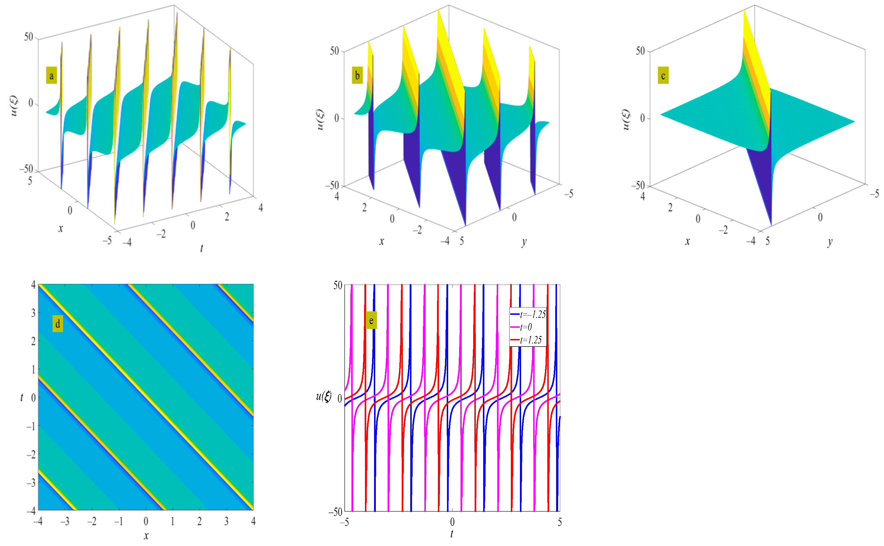
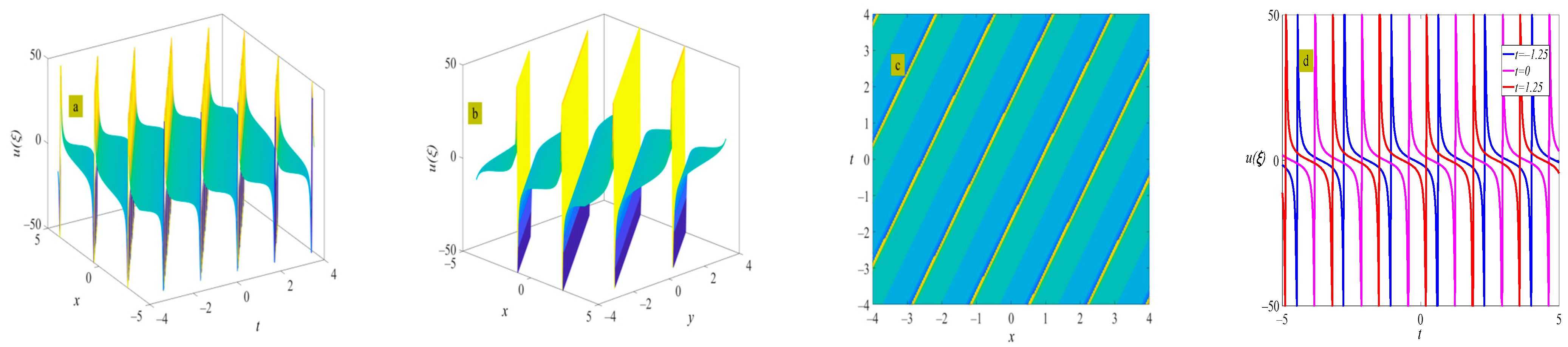
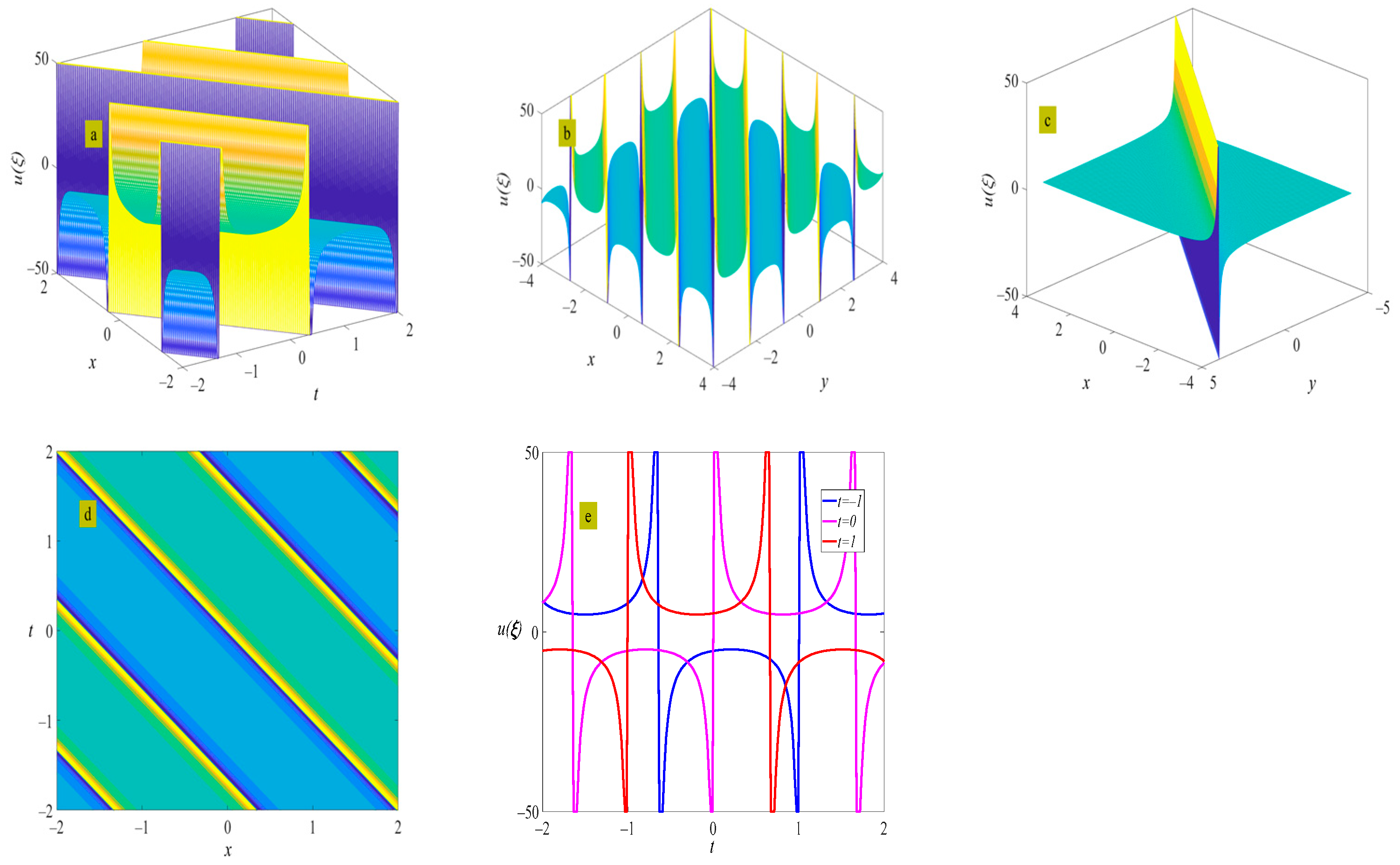
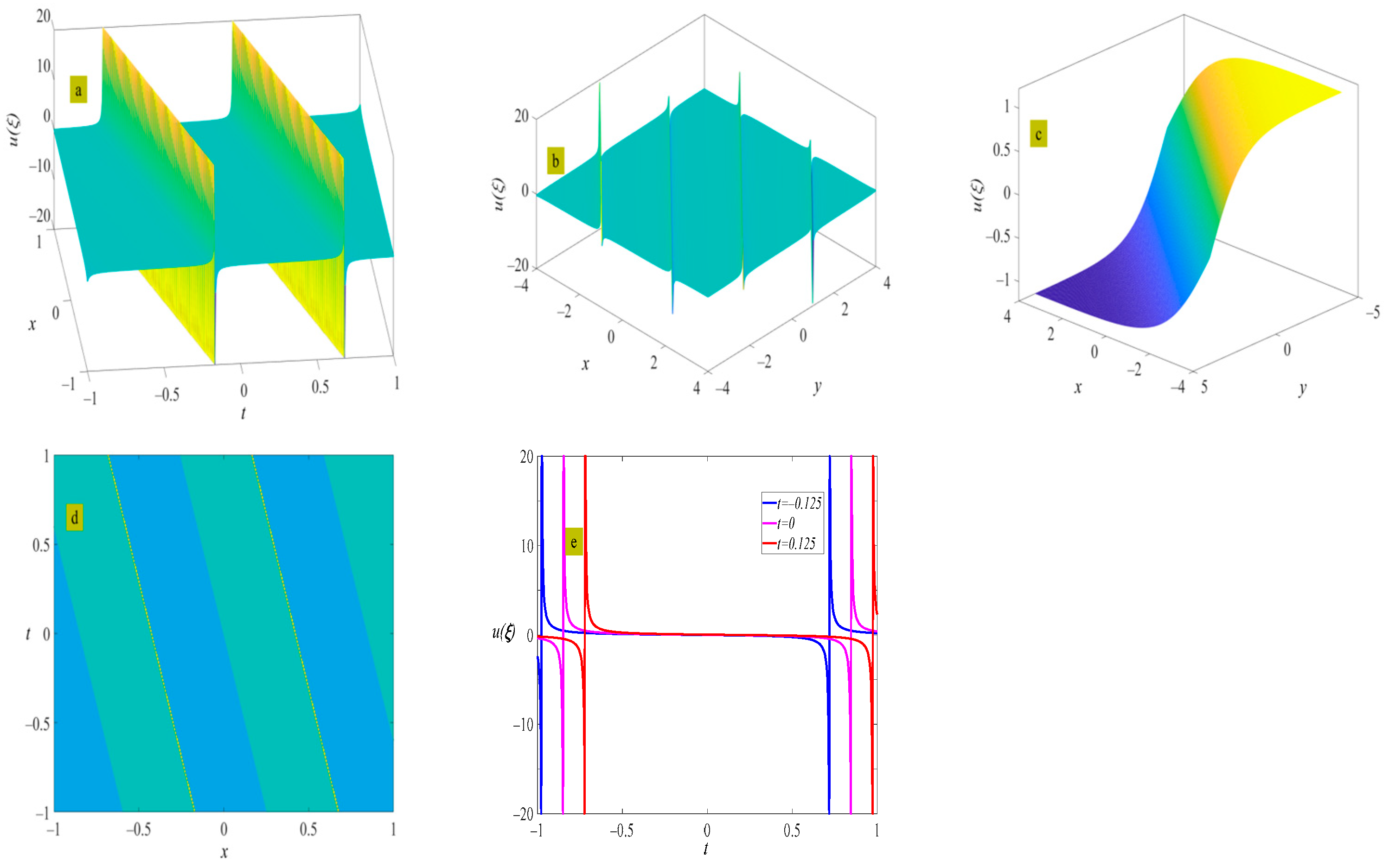
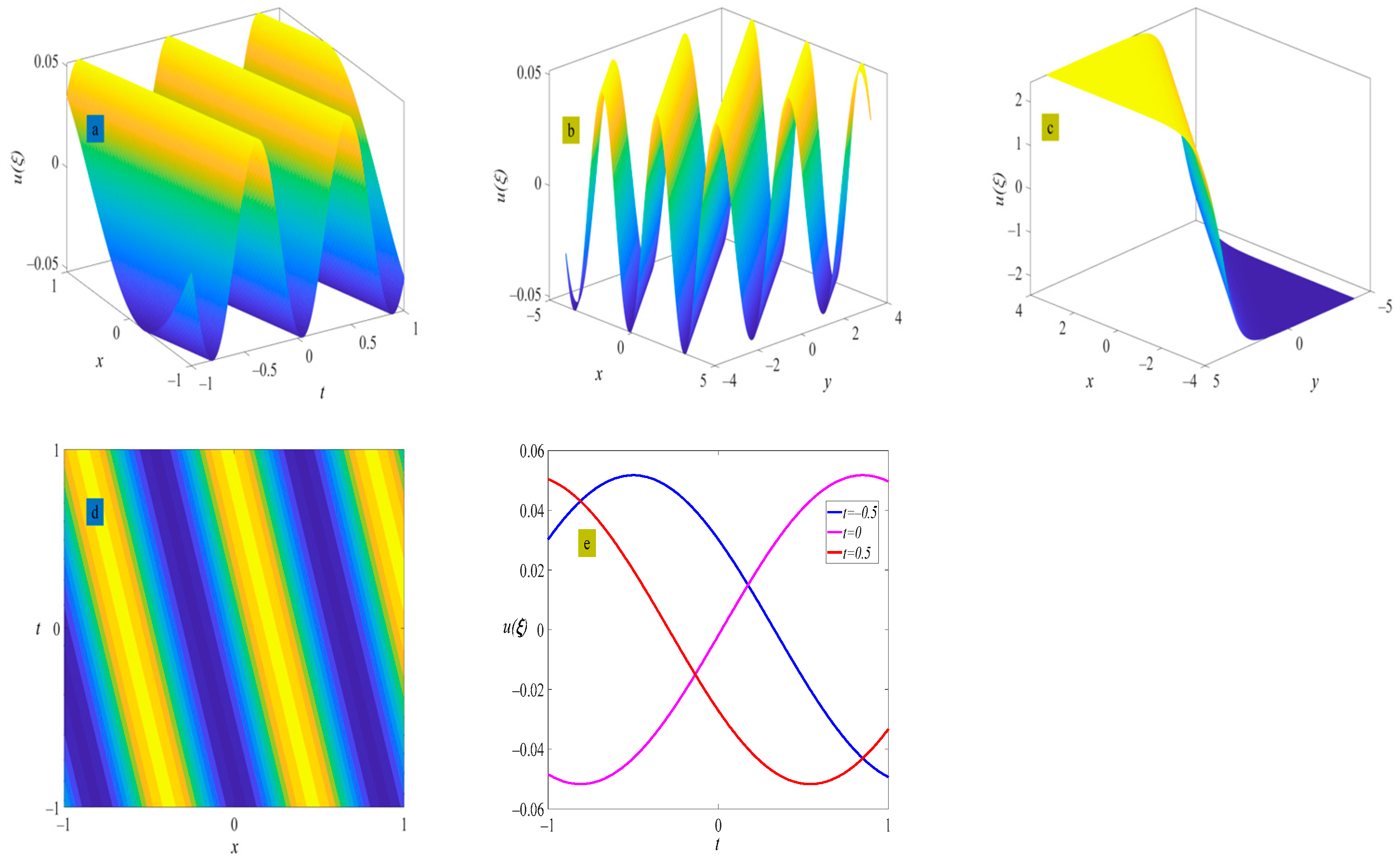
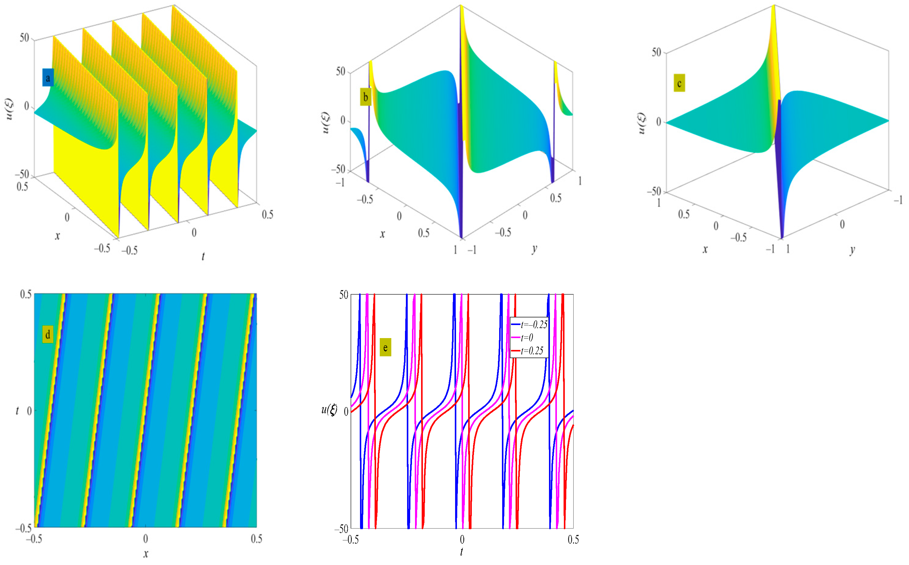
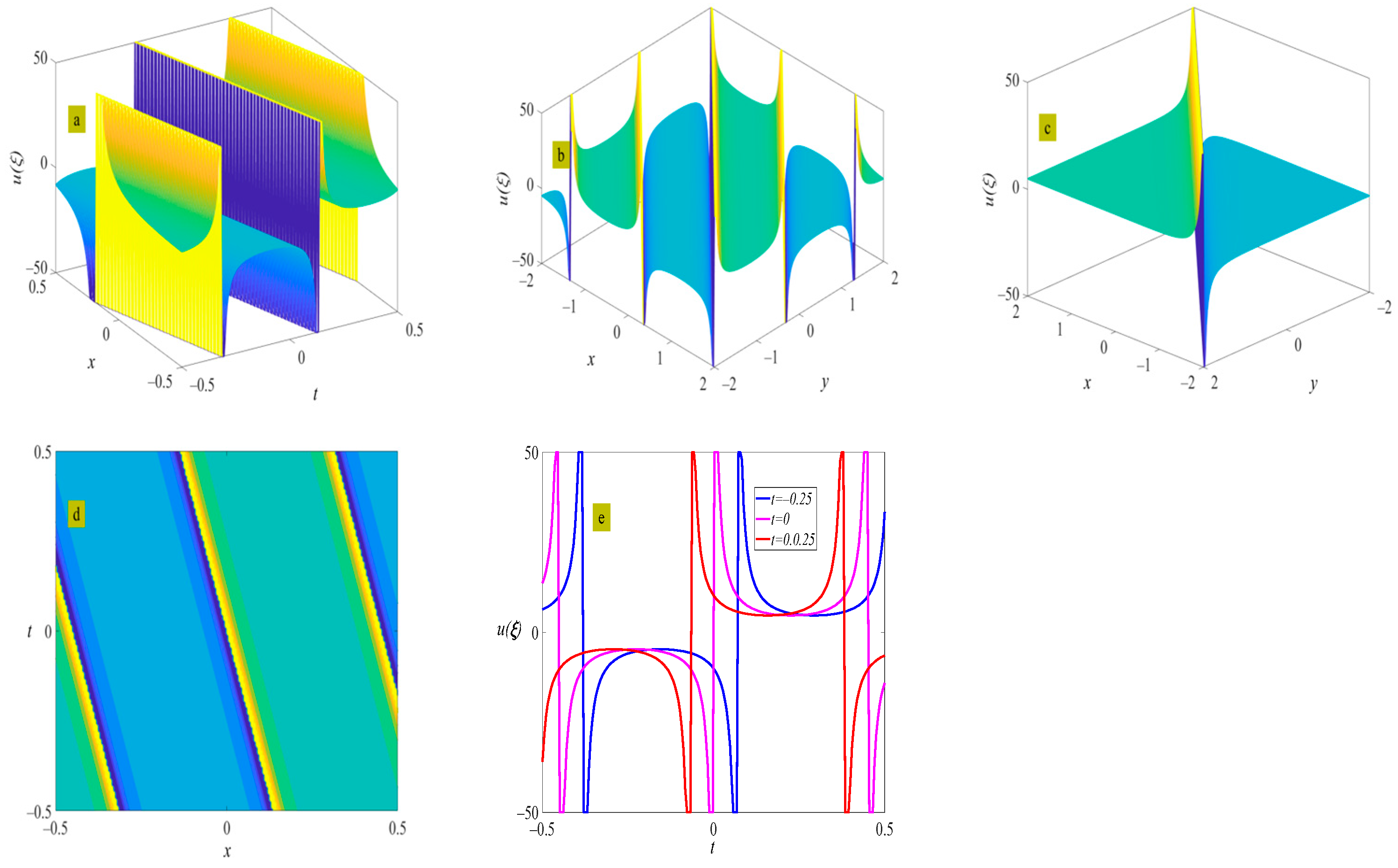
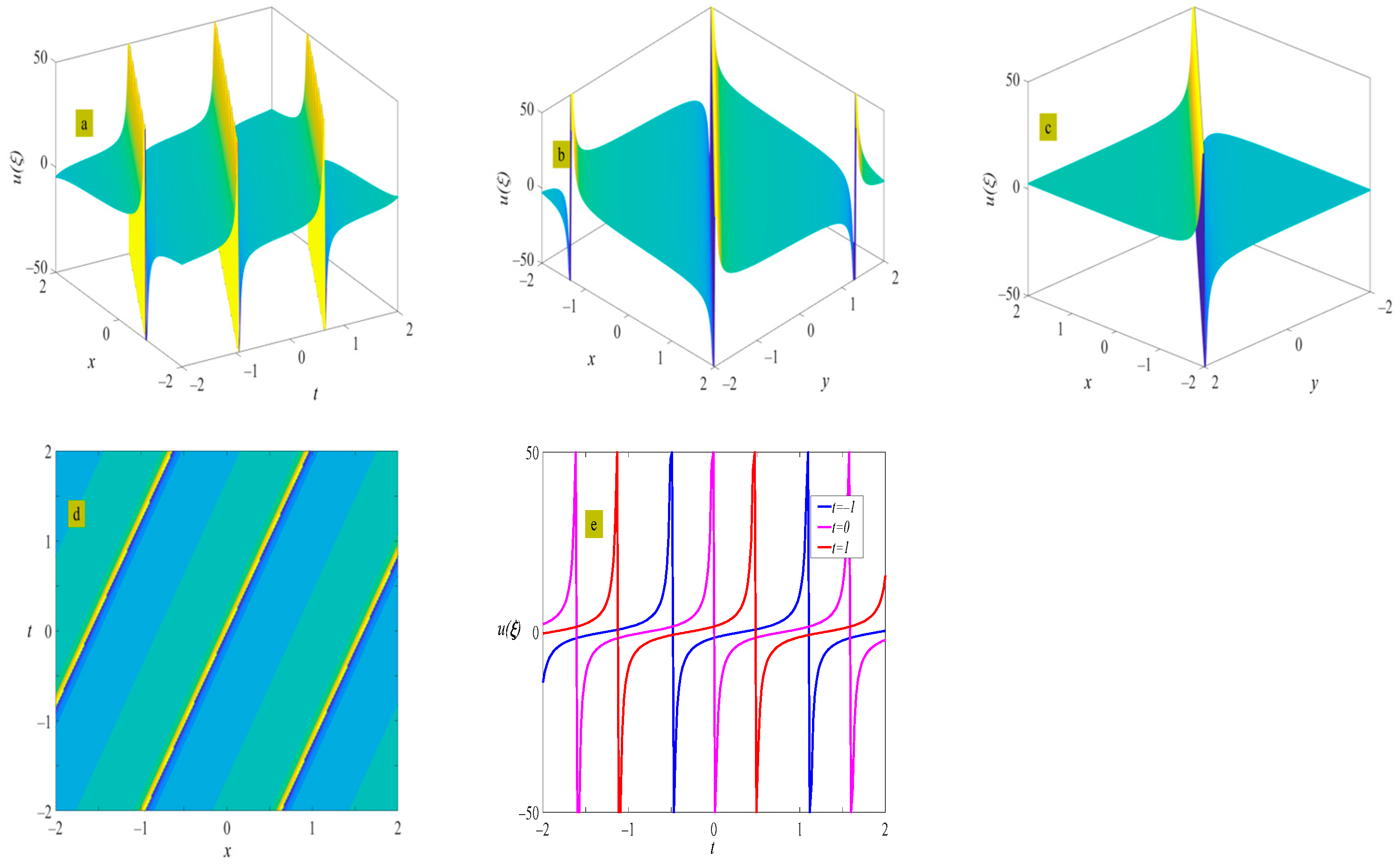
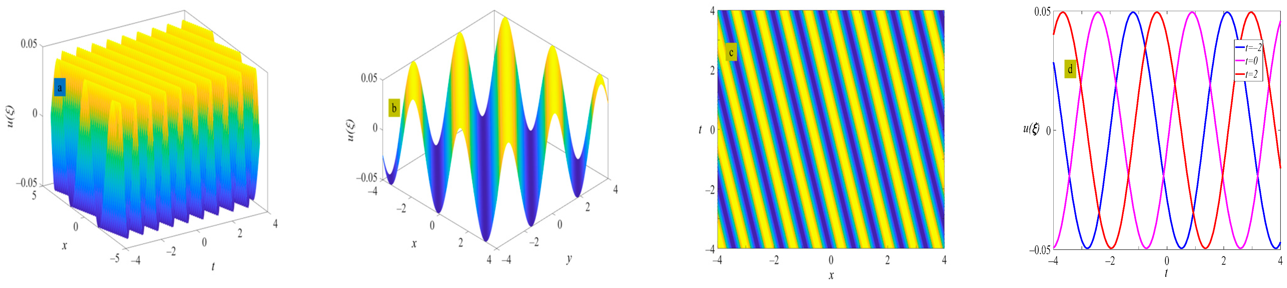
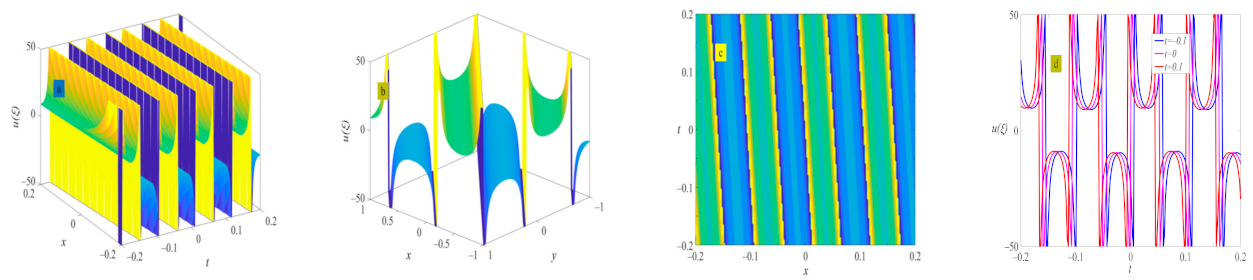
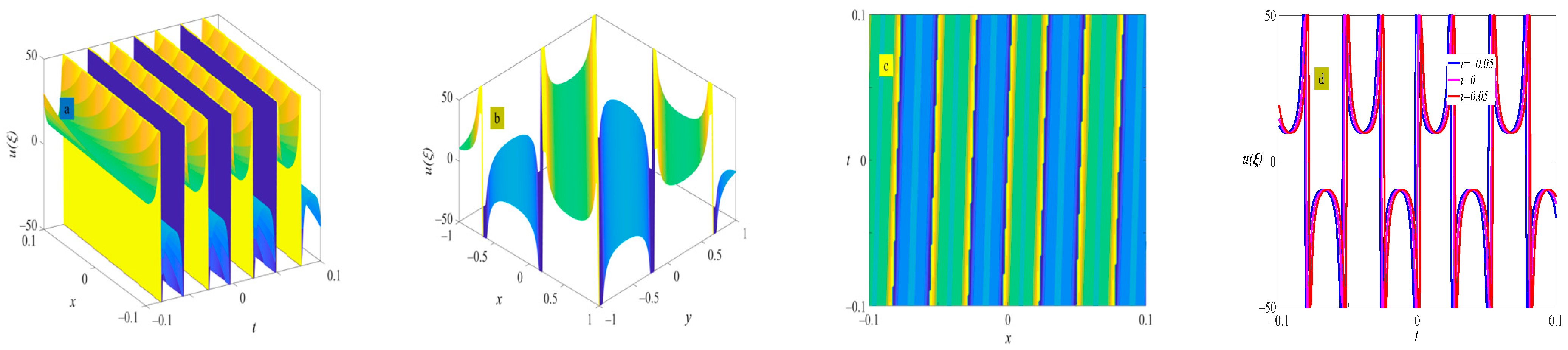
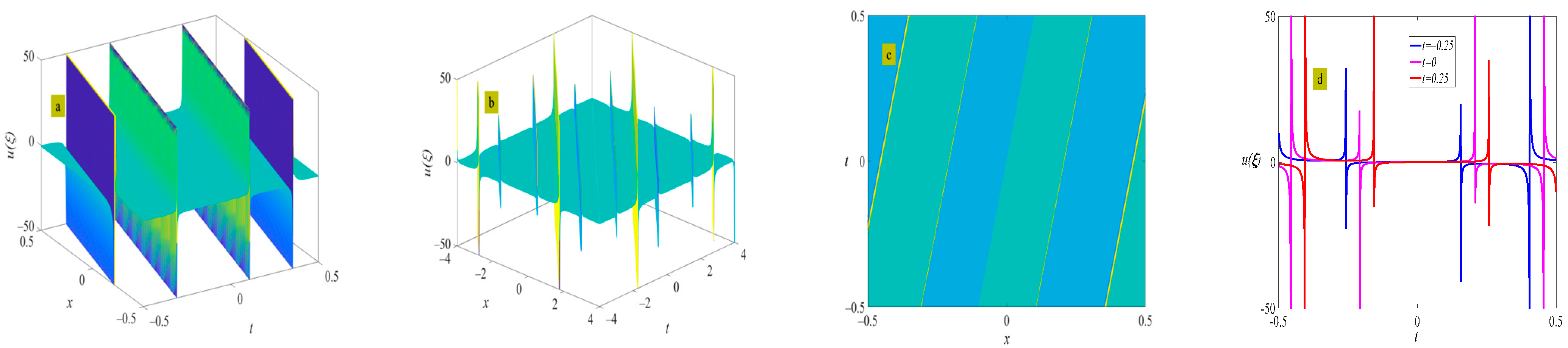
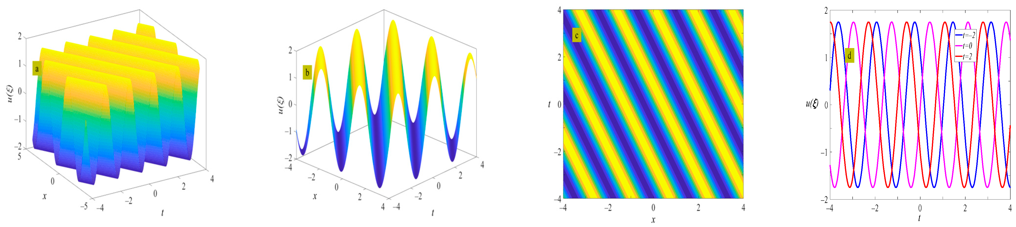
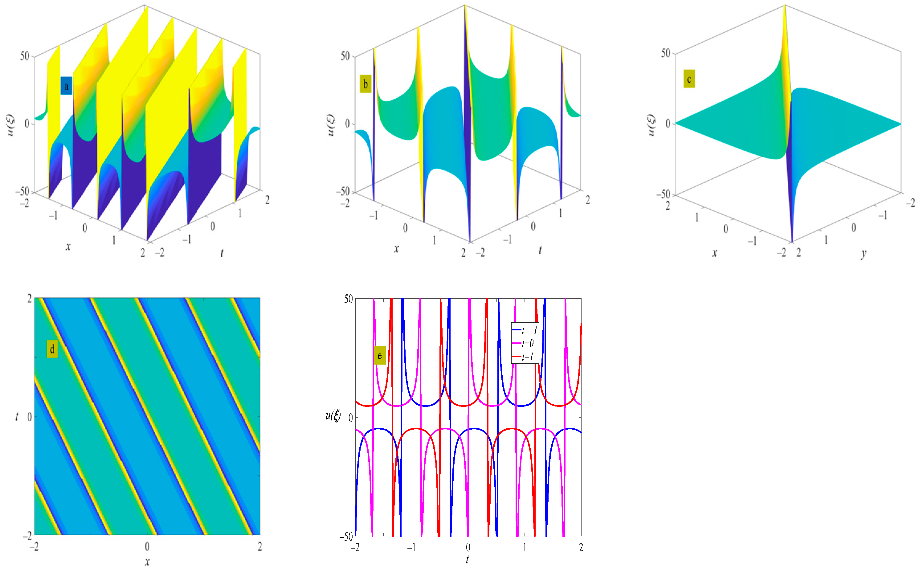
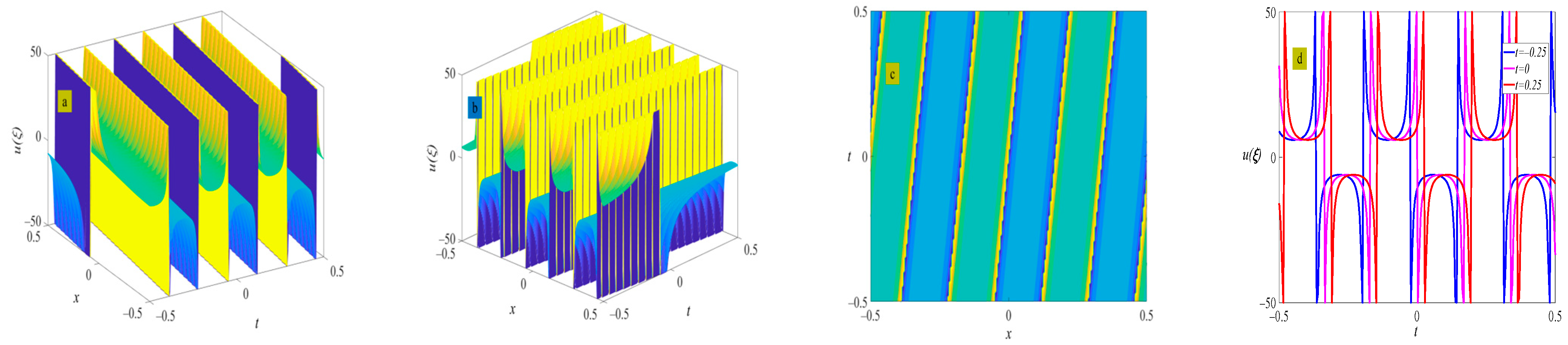
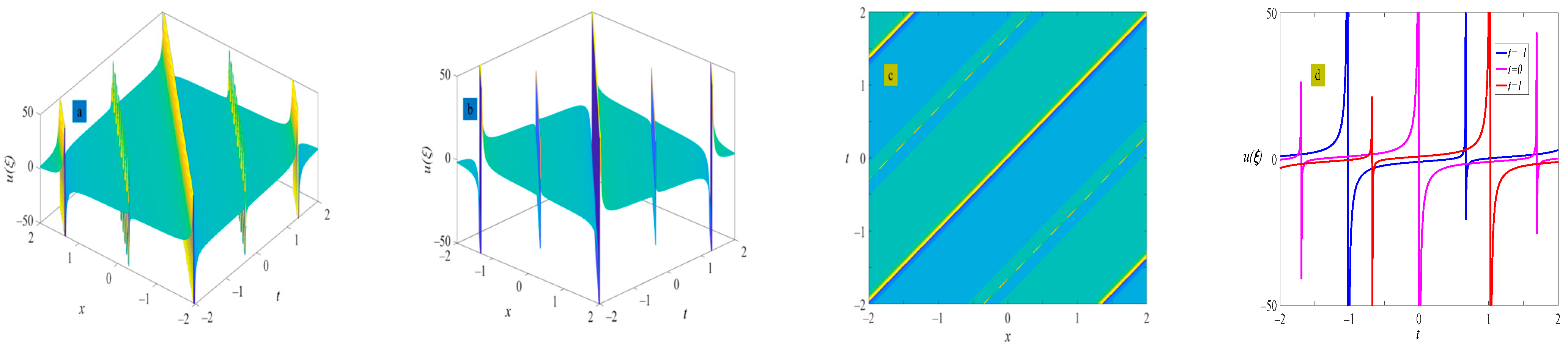
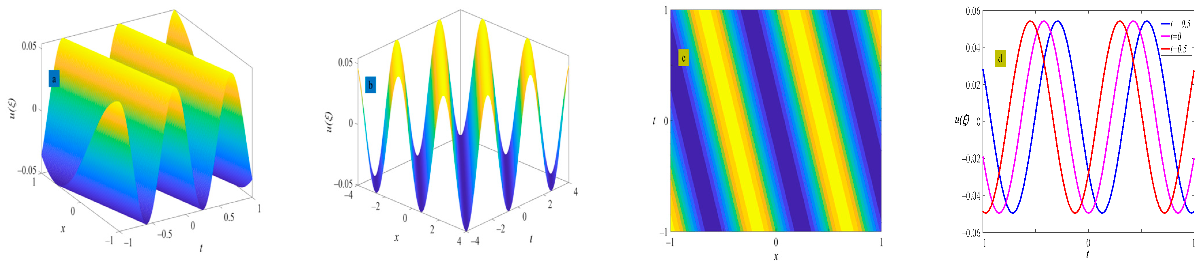
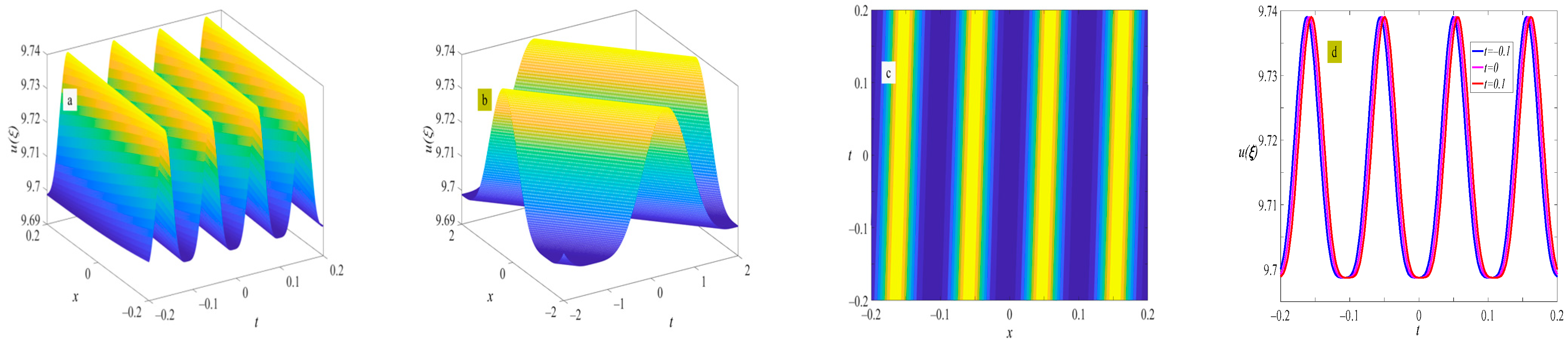
4. Example of the Solutions

To demonstrate the power and effectiveness of this method, a set of examples will be provided below. If $p_2={1-m}^2$, $q_2=2-m^2$, $r_2=1$, and $g\left(\xi \right)=sn(\xi )/cn(\xi )$, according to Equation (9), the solutions of the (3+1)-dimensional mKDV-ZK equation are shown as follows:

$$u_{11}\left(\xi \right)=\pm \sqrt{{\displaystyle \frac{6\omega }{(m^2-2)\alpha }}}{\displaystyle \frac{cn(\sigma \xi )}{sn(\sigma \xi )}},$$

(21)

where $\xi =x+y+z-\omega t,\sigma =\pm \sqrt{{\displaystyle \frac{\omega }{2-m^2}}}$. Figure 1 shows the evolution of the periodic wave represented by Equation (21), as well as the solitary wave at $m=1$. This is a periodic wave with singularities in specific spatiotemporal locations, and the amplitude and period of the wave remain unchanged during propagation.

$$u_{12}\left(\xi \right)=\pm \sqrt{{\displaystyle \frac{6(1-m^2)\omega }{(m^2-2)\alpha }}}{\displaystyle \frac{sn(\sigma \xi )}{cn(\sigma \xi )}},$$

(22)

where $\xi =x+y+z-\omega t,\sigma =\pm \sqrt{{\displaystyle \frac{\omega }{2-m^2}}}$. Figure 2 shows the evolution of the periodic wave represented by Equation (22). There are no solitary waves in this set of solutions because when m = 1, u(ξ) = 0.

$$u_{13}\left(\xi \right)=\pm \sqrt{{\displaystyle \frac{3\omega }{(2-m^2)\alpha }}}{\displaystyle \frac{dn(\sigma \xi )}{sn(\sigma \xi )cn(\sigma \xi )}},$$

(23)

where $\xi =x+y+z-\omega t,\sigma =\pm \sqrt{{\displaystyle \frac{\omega }{2(m^2-2)}}}$. Figure 3 shows the evolution of the periodic wave represented by Equation (23), as well as the solitary wave at $m=1$.

$$u_{14}\left(\xi \right)=\pm \sqrt{-{\displaystyle \frac{6\omega }{\left(2-m^2+6\lambda \sqrt{{1-m}^2}\right)\alpha }}}{\displaystyle \frac{cn\left(\sigma \xi \right)}{sn\left(\sigma \xi \right)}}\pm \sqrt{-{\displaystyle \frac{6({1-m}^2)\omega }{\left(2-m^2+6\lambda \sqrt{{1-m}^2}\right)\alpha }}}{\displaystyle \frac{sn\left(\sigma \xi \right)}{cn\left(\sigma \xi \right)}},$$

(24)

where $\xi =x+y+z-\omega t,\sigma =\pm \sqrt{{\displaystyle \frac{\omega }{2-m^2+6\lambda \sqrt{{1-m}^2}}}},{\lambda }^2=1$. Figure 4 shows the evolution of the periodic wave represented by Equation (24). When $m=1$, the solitary wave presented by Equation (24) is the same as that presented by Equation (21).

$$u_{15}\left(\xi \right)=\pm \sqrt{{\displaystyle \frac{3\omega }{\left[2-m^2+6\lambda \sqrt{{1-m}^2}\right]\alpha }}}\left[{\displaystyle \frac{cn\left(\sigma \xi \right)}{sn\left(\sigma \xi \right)}}\right]\pm \sqrt{{\displaystyle \frac{3({1-m}^2)\omega }{\left[2-m^2+6\lambda \sqrt{{1-m}^2}\right]\alpha }}}\left[{\displaystyle \frac{sn\left(\sigma \xi \right)}{cn\left(\sigma \xi \right)}}\right]\pm \sqrt{{\displaystyle \frac{3\omega }{\left[2-m^2+6\lambda \sqrt{{1-m}^2}\right]\alpha }}}\left[{\displaystyle \frac{dn(\sigma \xi )}{sn(\sigma \xi )cn(\sigma \xi )}}\right],$$

(25)

where $\xi =x+y+z-\omega t,\sigma =\pm \sqrt{-{\displaystyle \frac{2\omega }{2-m^2+6\lambda \sqrt{{1-m}^2}}}},{\lambda }^2=1$. Figure 5 shows the evolution of the periodic wave represented by Equation (25). When $m=1,$ the periodic wave degenerates into a kink solitary wave.

Due to the construction form of the solution in Equation (5), the solutions obtained in Equation (10) are the same as that in Equation (9). From Equation (11), the solutions of the (3+1)-dimensional mKDV-ZK equation are shown as follows:

$$u_{31}\left(\xi \right)=\pm \sqrt{{\displaystyle \frac{3m^4\omega }{(2-m^2)\alpha }}}\left[{\displaystyle \frac{sn\left(\sigma \xi \right)cn\left(\sigma \xi \right)}{dn\left(\sigma \xi \right)}}\right],$$

(26)

where $\xi =x+y+z-\omega t,\sigma =\pm \sqrt{{\displaystyle \frac{\omega }{-4+2m^2}}}$. Figure 6 shows the evolution of the periodic wave represented by Equation (26). When $m=1,$ the periodic wave degenerates into an anti-kink solitary wave.

$$u_{32}\left(\xi \right)=\pm \sqrt{{\displaystyle \frac{6\omega }{(4-2m^2)\alpha }}}\left[{\displaystyle \frac{dn\left(\sigma \xi \right)}{sn\left(\sigma \xi \right)cn\left(\sigma \xi \right)}}\right],$$

(27)

where $\xi =x+y+z-\omega t,\sigma =\pm \sqrt{{\displaystyle \frac{\omega }{-4+2m^2}}}$, which is the same as $u_{13}\left(\xi \right)$.

$$u_{33}\left(\xi \right)=\pm \sqrt{{\displaystyle \frac{3\omega }{(-4+2m^2)\alpha }}}\left[{\displaystyle \frac{m^2{cn}^4\left(\sigma \xi \right)+2(1-m^2){cn}^2\left(\sigma \xi \right)-(1-m^2)}{sn\left(\sigma \xi \right)cn\left(\sigma \xi \right)dn\left(\sigma \xi \right)}}\right],$$

(28)

where $\xi =x+y+z-\omega t,\sigma =\pm \sqrt{{\displaystyle \frac{\omega }{4(2-m^2)}}}$. Figure 7 shows the evolution of the periodic wave represented by Equation (28), as well as the solitary wave at $m=1$.

$$u_{34}\left(\xi \right)=\pm \sqrt{-{\displaystyle \frac{3m^4\omega }{(-2+m^2+3\lambda m^2)\alpha }}}\left[{\displaystyle \frac{sn\left(\sigma \xi \right)cn\left(\sigma \xi \right)}{dn\left(\sigma \xi \right)}}\right]\pm \sqrt{-{\displaystyle \frac{3\omega }{(-2+m^2+3\lambda m^2)\alpha }}}\left[{\displaystyle \frac{dn\left(\sigma \xi \right)}{sn\left(\sigma \xi \right)cn\left(\sigma \xi \right)}}\right],$$

(29)

where $\xi =x+y+z-\omega t,\sigma =\pm \sqrt{{\displaystyle \frac{\omega }{-4+2m^2+6\lambda m^2}}}$, ${\lambda }^2=1$. Figure 8 shows the evolution of the periodic wave represented by Equation (29), as well as the solitary wave at $m=1$.

$$u_{35}\left(\xi \right)=\pm \sqrt{{\displaystyle \frac{3m^4\omega }{(-4+2m^2+6\lambda m^2)\alpha }}}\left[{\displaystyle \frac{sn\left(\sigma \xi \right)cn\left(\sigma \xi \right)}{dn\left(\sigma \xi \right)}}\right]\pm \sqrt{{\displaystyle \frac{3\omega }{(-4+2m^2+6\lambda m^2)\alpha }}}\left[{\displaystyle \frac{dn\left(\sigma \xi \right)}{sn\left(\sigma \xi \right)cn\left(\sigma \xi \right)}}\right]\pm \sqrt{{\displaystyle \frac{3\omega }{(-4+2m^2+6\lambda m^2)\alpha }}}\left[{\displaystyle \frac{m^2{cn}^4\left(\sigma \xi \right)+2(1-m^2){cn}^2\left(\sigma \xi \right)-(1-m^2)}{sn\left(\sigma \xi \right)cn\left(\sigma \xi \right)dn\left(\sigma \xi \right)}}\right],$$

(30)

where $\xi =x+y+z-\omega t$, $\sigma =\pm \sqrt{-{\displaystyle \frac{2\omega }{-4+2m^2+6\lambda m^2}}}{,\lambda }^2=1$. Figure 9 shows the evolution of the periodic wave represented by Equation (30), as well as the solitary wave at $m=1$.

From Equation (12), the solutions of the (3+1)-dimensional mKDV-ZK equation are shown as follows:

$$u_{41}\left(\xi \right)=\pm \sqrt{-{\displaystyle \frac{6\left[8+4\lambda (2-m^2)\sqrt{\frac{1}{1-m^2}}\right]\omega }{(2-m^2+6\lambda \sqrt{{1-m}^2})\alpha }}}\left[{\displaystyle \frac{sn(\sigma \xi )cn(\sigma \xi )}{{sn}^2(\sigma \xi )-\lambda \sqrt{{1-m}^2}{cn}^2(\sigma \xi )}}\right],$$

(31)

where $\xi =x+y+z-\omega t,\sigma =\pm \sqrt{{\displaystyle \frac{\omega }{2-m^2+6\lambda \sqrt{{1-m}^2}}}}{,\lambda }^2=1$. Figure 10 shows the evolution of the periodic wave represented by Equation (31). There is no solitary wave solution for this set of solutions.

$$u_{42}\left(\xi \right)=\pm \sqrt{-{\displaystyle \frac{6({1-m}^2)\omega }{(2-m^2+6\lambda \sqrt{{1-m}^2})\alpha }}}\left[{\displaystyle \frac{{sn}^2(\sigma \xi )-\lambda \sqrt{{1-m}^2}{cn}^2(\sigma \xi )}{sn(\sigma \xi )cn(\sigma \xi )}}\right],$$

(32)

where $\xi =x+y+z-\omega t$, $\sigma =\pm \sqrt{{\displaystyle \frac{\omega }{2-m^2+6\lambda \sqrt{{1-m}^2}}}}$, which is the same as $u_{14}\left(\xi \right)$.

$$u_{43}\left(\xi \right)=\pm \sqrt{{\displaystyle \frac{3\omega }{(2-m^2+6\lambda \sqrt{{1-m}^2})\alpha }}}\left[{\displaystyle \frac{{-sn}^2(\sigma \xi )dn(\sigma \xi )-\lambda \sqrt{\frac{1}{1-m^2}}{cn}^2(\sigma \xi )dn(\sigma \xi )}{{sn}^3(\sigma \xi )cn(\sigma \xi )-\lambda \sqrt{\frac{1}{1-m^2}}sn(\sigma \xi ){cn}^3(\sigma \xi )}}\right],$$

(33)

where $\xi =x+y+z-\omega t$, $\sigma =\pm \sqrt{-{\displaystyle \frac{\omega }{2(2-m^2+6\lambda \sqrt{{1-m}^2})}}}{,\lambda }^2=1$. Figure 11 shows the evolution of the periodic wave represented by Equation (33).

$$u_{44}\left(\xi \right)=\pm \sqrt{-{\displaystyle \frac{6\left[8+4\lambda (2-m^2)\sqrt{\frac{1}{1-m^2}}\right]\omega }{\left[2-m^2+6\lambda \sqrt{{1-m}^2}\pm 6\sqrt{8(1-m^2)+4\lambda (2-m^2)\sqrt{1-m^2}}\right]\alpha }}}\left[{\displaystyle \frac{sn(\sigma \xi )cn(\sigma \xi )}{{sn}^2(\sigma \xi )-\lambda \sqrt{{1-m}^2}{cn}^2(\sigma \xi )}}\right]\pm \sqrt{-{\displaystyle \frac{6({1-m}^2)\omega }{\left[2-m^2+6\lambda \sqrt{{1-m}^2}\pm 6\sqrt{8(1-m^2)+4\lambda (2-m^2)\sqrt{1-m^2}}\right]\alpha }}}\left[{\displaystyle \frac{{sn}^2(\sigma \xi )-\lambda \sqrt{{1-m}^2}{cn}^2(\sigma \xi )}{sn(\sigma \xi )cn(\sigma \xi )}}\right],$$

(34)

where $\xi =x+y+z-\omega t,\sigma =\pm \sqrt{{\displaystyle \frac{\omega }{-2-m^2+6\lambda \sqrt{{1-m}^2}\pm 6\sqrt{8(1-m^2)+4\lambda (2-m^2)\sqrt{1-m^2}}}}}{,\lambda }^2=1$. Figure 12 shows the evolution of the periodic wave represented by Equation (34).

$$u_{45}\left(\xi \right)=\pm \sqrt{{\displaystyle \frac{3\left[8+4\lambda (2-m^2)\sqrt{\frac{1}{1-m^2}}\right]\omega }{\left[2-m^2+6\lambda \sqrt{{1-m}^2}\pm 6\sqrt{8(1-m^2)+4\lambda (2-m^2)\sqrt{1-m^2}}\right]\alpha }}}\left[{\displaystyle \frac{sn(\sigma \xi )cn(\sigma \xi )}{{sn}^2(\sigma \xi )-\lambda \sqrt{{1-m}^2}{cn}^2(\sigma \xi )}}\right]\pm \sqrt{{\displaystyle \frac{3({1-m}^2)\omega }{\left[2-m^2+6\lambda \sqrt{{1-m}^2}\pm 6\sqrt{8(1-m^2)+4\lambda (2-m^2)\sqrt{1-m^2}}\right]\alpha }}}\left[{\displaystyle \frac{{sn}^2(\sigma \xi )-\lambda \sqrt{{1-m}^2}{cn}^2(\sigma \xi )}{sn(\sigma \xi )cn(\sigma \xi )}}\right]\pm \sqrt{{\displaystyle \frac{3\omega }{\left[2-m^2+6\lambda \sqrt{{1-m}^2}\pm 6\sqrt{8(1-m^2)+4\lambda (2-m^2)\sqrt{1-m^2}}\right]\alpha }}}\left[{\displaystyle \frac{{-sn}^2(\sigma \xi )dn(\sigma \xi )-\lambda \sqrt{\frac{1}{1-m^2}}{cn}^2(\sigma \xi )dn(\sigma \xi )}{{sn}^3(\sigma \xi )cn(\sigma \xi )-\lambda \sqrt{\frac{1}{1-m^2}}sn(\sigma \xi ){cn}^3(\sigma \xi )}}\right],$$

(35)

where $\xi =x+y+z-\omega t$, $\sigma =\pm \sqrt{-{\displaystyle \frac{2\omega }{2-m^2+6\lambda \sqrt{{1-m}^2}\pm 6\sqrt{8(1-m^2)+4\lambda (2-m^2)\sqrt{1-m^2}}}}}{,\lambda }^2=1$. Figure 13 shows the evolution of the periodic wave represented by Equation (35).

From Equation (13), the solutions of the (3+1)-dimensional mKDV-ZK equation are shown as follows:

$$u_{51}\left(\xi \right)=\pm \sqrt{-{\displaystyle \frac{6\left[1-m^2-\frac{3}{4}{(2-m^2)}^2+3(2-m^2)\sqrt{1-m^2}\right]\omega }{\left[\frac{1}{2}(2-m^2)+3\sqrt{1-m^2}\right]\alpha }}}\left[{\displaystyle \frac{sn(\sigma \xi )cn(\sigma \xi )}{\pm \sqrt{1-m^2}{sn}^2\left(\sigma \xi \right)+dn(\sigma \xi )\pm {cn}^2\left(\sigma \xi \right)}}\right],$$

(36)

where $\xi =x+y+z-\omega t,\sigma =\pm \sqrt{{\displaystyle \frac{\omega }{\frac{1}{2}(2-m^2)+3\sqrt{1-m^2}}}}$. Figure 14 shows the evolution of the periodic wave represented by Equation (36). There is no solitary wave solution for this set of solutions.

$$u_{52}\left(\xi \right)=\pm \sqrt{-{\displaystyle \frac{3\omega }{\left[(2-m^2)+6\sqrt{1-m^2}\right]\alpha }}}\left[{\displaystyle \frac{\pm \sqrt{1-m^2}{sn}^2\left(\sigma \xi \right)+dn(\sigma \xi )\pm {cn}^2\left(\sigma \xi \right)}{sn(\sigma \xi )cn(\sigma \xi )}}\right],$$

(37)

where $\xi =x+y+z-\omega t,\sigma =\pm \sqrt{{\displaystyle \frac{\omega }{\frac{1}{2}(2-m^2)+3\sqrt{1-m^2}}}}$. Figure 15 shows the evolution of the periodic wave and solitary wave at $m=1$ represented by Equation (37).

$$u_{53}\left(\xi \right)=\pm \sqrt{{\displaystyle \frac{3\omega }{\left[\frac{1}{2}(2-m^2)+3\sqrt{1-m^2}\right]\alpha }}}\left[{\displaystyle \frac{\mp {sn}^2(\sigma \xi )dn(\sigma \xi )-(1-m^2){sn}^4(\sigma \xi )\pm {cn}^2\left(\sigma \xi \right)dn(\sigma \xi )}{\pm \sqrt{1-m^2}{sn}^3\left(\sigma \xi \right)cn(\sigma \xi )+sn(\sigma \xi )cn(\sigma \xi )dn(\sigma \xi )\pm sn(\sigma \xi ){cn}^3\left(\sigma \xi \right)}}\right],$$

(38)

where $\xi =x+y+z-\omega t,\sigma =\pm \sqrt{-{\displaystyle \frac{\omega }{(2-m^2)+6\sqrt{1-m^2}}}}$. Figure 16 shows the evolution of the periodic wave and solitary wave at $m=1$ represented by Equation (38).

$$u_{54}\left(\xi \right)=\pm \sqrt{-{\displaystyle \frac{6\left[1-m^2-\frac{3}{4}{(2-m^2)}^2+3(2-m^2)\sqrt{1-m^2}\right]\omega }{\left[\frac{1}{2}(2-m^2)+3\sqrt{1-m^2}\pm 3\sqrt{1-m^2-\frac{3}{4}{(2-m^2)}^2+3(2-m^2)\sqrt{1-m^2}}\right]\alpha }}}\left[{\displaystyle \frac{sn(\sigma \xi )cn(\sigma \xi )}{\pm \sqrt{1-m^2}{sn}^2\left(\sigma \xi \right)+dn(\sigma \xi )\pm {cn}^2\left(\sigma \xi \right)}}\right]\pm \sqrt{-{\displaystyle \frac{3\omega }{\left[(2-m^2)+6\sqrt{1-m^2}\pm 6\sqrt{1-m^2-\frac{3}{4}{(2-m^2)}^2+3(2-m^2)\sqrt{1-m^2}}\right]\alpha }}}\left[{\displaystyle \frac{\pm \sqrt{1-m^2}{sn}^2\left(\sigma \xi \right)+dn(\sigma \xi )\pm {cn}^2\left(\sigma \xi \right)}{sn(\sigma \xi )cn(\sigma \xi )}}\right],$$

(39)

where $\xi =x+y+z-\omega t,\sigma =\pm \sqrt{{\displaystyle \frac{\omega }{\frac{1}{2}(2-m^2)+3\sqrt{1-m^2}\pm 3\sqrt{1-m^2-\frac{3}{4}{(2-m^2)}^2+3(2-m^2)\sqrt{1-m^2}}}}}$. Figure 17 shows the evolution of the periodic wave represented by Equation (39). There is no solitary wave solution for this set of solutions.

$$u_{55}\left(\xi \right)=-\pm \sqrt{-{\displaystyle \frac{3\left[1-m^2-\frac{3}{4}{(2-m^2)}^2+3(2-m^2)\sqrt{1-m^2}\right]\omega }{\left[\frac{1}{2}(2-m^2)+3\sqrt{1-m^2}\pm 3\sqrt{1-m^2-\frac{3}{4}{(2-m^2)}^2+3(2-m^2)\sqrt{1-m^2}}\right]\alpha }}}\left[{\displaystyle \frac{sn(\sigma \xi )cn(\sigma \xi )}{\pm \sqrt{1-m^2}{sn}^2\left(\sigma \xi \right)+dn(\sigma \xi )\pm {cn}^2\left(\sigma \xi \right)}}\right]\pm \sqrt{-{\displaystyle \frac{3\omega }{2\left[(2-m^2)+6\sqrt{1-m^2}\pm 6\sqrt{1-m^2-\frac{3}{4}{(2-m^2)}^2+3(2-m^2)\sqrt{1-m^2}}\right]\alpha }}}\left[{\displaystyle \frac{\pm \sqrt{1-m^2}{sn}^2\left(\sigma \xi \right)+dn(\sigma \xi )\pm {cn}^2\left(\sigma \xi \right)}{sn(\sigma \xi )cn(\sigma \xi )}}\right]\pm \sqrt{-{\displaystyle \frac{3\omega }{\left[\frac{1}{2}(2-m^2)+3\sqrt{1-m^2}\pm 3\sqrt{1-m^2-\frac{3}{4}{(2-m^2)}^2+3(2-m^2)\sqrt{1-m^2}}\right]\alpha }}}\left[{\displaystyle \frac{\mp {sn}^2(\sigma \xi )dn(\sigma \xi )-(1-m^2){sn}^4(\sigma \xi )\pm {cn}^2\left(\sigma \xi \right)dn(\sigma \xi )}{\pm \sqrt{1-m^2}{sn}^3\left(\sigma \xi \right)cn(\sigma \xi )+sn(\sigma \xi )cn(\sigma \xi )dn(\sigma \xi )\pm sn(\sigma \xi ){cn}^3\left(\sigma \xi \right)}}\right],$$

(40)

where $\xi =x+y+z-\omega t,\sigma =\pm \sqrt{-{\displaystyle \frac{2\omega }{\frac{1}{2}(2-m^2)+3\sqrt{1-m^2}\pm 3\sqrt{1-m^2-\frac{3}{4}{(2-m^2)}^2+3(2-m^2)\sqrt{1-m^2}}}}}$. Figure 18 shows the evolution of the periodic wave represented by Equation (40). There is no solitary wave solution for this set of solutions.

From Equation (15), the solutions of the (3+1)-dimensional mKDV-ZK equation are shown as follows:

$$u_{61}\left(\xi \right)=\pm \sqrt{-{\displaystyle \frac{24\lambda \omega }{\sqrt{1-m^2}(2-m^2-6\lambda \sqrt{1-m^2})\alpha }}}\left[{\displaystyle \frac{dn(\sigma \xi )}{{sn}^2\left(\sigma \xi \right)-\lambda \sqrt{\frac{1}{1-m^2}}{cn}^2\left(\sigma \xi \right)}}\right],$$

(41)

where $\xi =x+y+z-\omega t,\sigma =\pm \sqrt{{\displaystyle \frac{\omega }{2-m^2-6\lambda \sqrt{1-m^2}}}}{,\lambda }^2=1$. Figure 19 shows the evolution of the periodic wave represented by Equation (41). There is no solitary wave solution for this set of solutions.

$$u_{62}\left(\xi \right)=\pm \sqrt{-{\displaystyle \frac{6[-(1-m^2)(2-m^2)+2\lambda (1-m^2)\sqrt{1-m^2}]\omega }{(2-m^2-6\lambda \sqrt{1-m^2})\alpha }}}\left[{\displaystyle \frac{{sn}^2\left(\sigma \xi \right)-\lambda \sqrt{\frac{1}{1-m^2}}{cn}^2\left(\sigma \xi \right)}{dn(\sigma \xi )}}\right],$$

(42)

where $\xi =x+y+z-\omega t,\sigma =\pm \sqrt{{\displaystyle \frac{\omega }{2-m^2-6\lambda \sqrt{1-m^2}}}}{,\lambda }^2=1$. Figure 20 shows the evolution of the periodic wave represented by Equation (42). There is no solitary wave solution for this set of solutions.

$$u_{63}\left(\xi \right)=\pm \sqrt{{\displaystyle \frac{3\omega }{(2-m^2-6\lambda \sqrt{1-m^2})\alpha }}}\left[{\displaystyle \frac{(-2\lambda \sqrt{1-m^2}-2+m^2){sn}^3\left(\sigma \xi \right)cn(\sigma \xi )-(2-m^2)\lambda \sqrt{\frac{1}{1-m^2}}{{sn}^2\left(\sigma \xi \right)cn}^2\left(\sigma \xi \right)+{sn}^4\left(\sigma \xi \right)}{{sn}^2\left(\sigma \xi \right)dn(\sigma \xi )-\lambda \sqrt{\frac{1}{1-m^2}}{cn}^2\left(\sigma \xi \right)}}\right],$$

(43)

where $\xi =x+y+z-\omega t,\sigma =\pm \sqrt{-{\displaystyle \frac{\omega }{2(2-m^2-6\lambda \sqrt{1-m^2})}}}{,\lambda }^2=1$. The evolution of the periodic wave represented by Equation (43) is shown in Figure 21.

$$u_{64}\left(\xi \right)=\pm \sqrt{-{\displaystyle \frac{24\lambda \omega }{\sqrt{1-m^2}\left[2-m^2-6\lambda \sqrt{1-m^2}\pm 12\sqrt{-(2-m^2)\lambda \sqrt{1-m^2}+2(1-m^2)}\right]\alpha }}}\left[{\displaystyle \frac{dn(\sigma \xi )}{{sn}^2\left(\sigma \xi \right)-\lambda \sqrt{\frac{1}{1-m^2}}{cn}^2\left(\sigma \xi \right)}}\right]\pm \sqrt{-{\displaystyle \frac{6[-(1-m^2)(2-m^2)+2\lambda (1-m^2)\sqrt{1-m^2}]\omega }{\left[2-m^2-6\lambda \sqrt{1-m^2}\pm 12\sqrt{-(2-m^2)\lambda \sqrt{1-m^2}+2(1-m^2)}\right]\alpha }}}\left[{\displaystyle \frac{{sn}^2\left(\sigma \xi \right)-\lambda \sqrt{\frac{1}{1-m^2}}{cn}^2\left(\sigma \xi \right)}{dn(\sigma \xi )}}\right],$$

(44)

where $\xi =x+y+z-\omega t,\sigma =\pm \sqrt{{\displaystyle \frac{\omega }{2-m^2-6\lambda \sqrt{1-m^2}\pm 12\sqrt{-(2-m^2)\lambda \sqrt{1-m^2}+2(1-m^2)}}}}{,\lambda }^2=1$. The evolution of the periodic wave represented by Equation (44) is shown in Figure 22.

$$u_{65}\left(\xi \right)=\pm \sqrt{{\displaystyle \frac{12\lambda \omega }{\sqrt{1-m^2}\left[2-m^2-6\lambda \sqrt{1-m^2}\pm 12\sqrt{-(2-m^2)\lambda \sqrt{1-m^2}+2(1-m^2)}\right]\alpha }}}\left[{\displaystyle \frac{dn(\sigma \xi )}{{sn}^2\left(\sigma \xi \right)-\lambda \sqrt{\frac{1}{1-m^2}}{cn}^2\left(\sigma \xi \right)}}\right]\pm \sqrt{{\displaystyle \frac{3[-(1-m^2)(2-m^2)+2\lambda (1-m^2)\sqrt{1-m^2}]\omega }{\left[2-m^2-6\lambda \sqrt{1-m^2}\pm 12\sqrt{-(2-m^2)\lambda \sqrt{1-m^2}+2(1-m^2)}\right]\alpha }}}\left[{\displaystyle \frac{{sn}^2\left(\sigma \xi \right)-\lambda \sqrt{\frac{1}{1-m^2}}{cn}^2\left(\sigma \xi \right)}{dn(\sigma \xi )}}\right]\pm \sqrt{{\displaystyle \frac{3\omega }{\left[2-m^2-6\lambda \sqrt{1-m^2}\pm 12\sqrt{-(2-m^2)\lambda \sqrt{1-m^2}+2(1-m^2)}\right]\alpha }}}\left[{\displaystyle \frac{(-2\lambda \sqrt{1-m^2}-2+m^2){sn}^3\left(\sigma \xi \right)cn(\sigma \xi )-(2-m^2)\lambda \sqrt{\frac{1}{1-m^2}}{{sn}^2\left(\sigma \xi \right)cn}^2\left(\sigma \xi \right)+{sn}^4\left(\sigma \xi \right)}{{sn}^2\left(\sigma \xi \right)dn(\sigma \xi )-\lambda \sqrt{\frac{1}{1-m^2}}{cn}^2\left(\sigma \xi \right)}}\right],$$

(45)

where $\xi =x+y+z-\omega t,\sigma =\pm \sqrt{-{\displaystyle \frac{2\omega }{2-m^2-6\lambda \sqrt{1-m^2}\pm 12\sqrt{-(2-m^2)\lambda \sqrt{1-m^2}+2(1-m^2)}}}}{,\lambda }^2=1$ This set of solutions represents the traveling wave solutions of Equation (3) in complex space.

The (3+1)-dimensional mKDV-ZK equation still has a large number of new types of periodic wave solutions, which may also include corresponding hyperbolic and trigonometric function solutions according to Equations (9)–(20) and Table 1. Due to space limitations, we will not provide examples one by one.

5. Discussion and Conclusions

The solutions obtained in this article can be used to describe the propagation of nonlinear waves in fluid dynamics, nonlinear optics, quantum mechanics, and so on. To provide an intuitive understanding of the structure of nonlinear waves and their propagation in time and space, we set the parameters of the (3+1)-dimensional mKDV-ZK equation and traveling wave to given values and apply mathematical software Matlab2021b to draw three-dimensional and two-dimensional contour plots of some solutions (see Figure 1, Figure 2, Figure 3, Figure 4, Figure 5, Figure 6, Figure 7, Figure 8, Figure 9, Figure 10, Figure 11, Figure 12, Figure 13, Figure 14, Figure 15, Figure 16, Figure 17, Figure 18, Figure 19, Figure 20, Figure 21 and Figure 22). These waves exhibit kink solitons, anti-kink solitons, and nonlinear waves propagating in spacetime periodically. Different parameters of the (3+1)-dimensional mKDV-ZK equation, different traveling wave parameters, and different structures of the solutions can cause different changes in the types, amplitude, and period of these nonlinear waves. For example, Figure 6 depicts a (3+1)-dimensional spatiotemporal evolution periodic wave with an amplitude of 0.05 and a wave velocity of −3.92 in the (3+1)-dimensional mKDV-ZK. When m $\to$ 1, the periodic wave degenerates into an anti-kink type solitary wave with an amplitude of 2.8 and a wave velocity of −3.92. This indicates the existence of periodic waves and solitary waves with this characteristic in fluid, fiber optic communication, optical waveguides, and quantum systems, and it can also be seen from Figure 6 that the shape, amplitude, and velocity of these nonlinear waves remain unchanged during propagation. It should be noted that we only provided images in the (x, t) and (x, y) phase spaces but did not provide images in the z-related spaces. It is consistent with images in the x-related and y-related spaces.

This article utilizes two new techniques to deal with the Jacobian elliptic equation and constructs new periodic wave solutions for the (3+1)-dimensional mKDV-ZK equation. This is a new expansion method proposed by us first, resulting in a large number of new types of Jacobian elliptic function solutions for the (3+1)-dimensional mKDV-ZK equation, including trigonometric function solutions and hyperbolic function solutions yet. Some new types of solutions have not been found in previous work. These results contribute to understanding the propagation of nonlinear waves in fields such as fluid dynamics, nonlinear optics, and quantum mechanics and expand our knowledge in these fields. The numerical images of some solutions show that these periodic waves exhibit complex nonlinear wave phenomena.

References

1. Wazwaz, A.M. The extended tanh method for new compact and noncompact solutions for the KP–BBM and the ZK–BBM equations. Chaos Solitons Fractals 2008, 38, 1505. [Google Scholar] [CrossRef]
2. Yusofoǧlu, E. New solitonary solutions for the MBBM equations using Exp-function method. Phys. Lett. A 2008, 372, 442. [Google Scholar] [CrossRef]
3. Gardner, C.S.; Greene, J.M.; Kruskal, M.D.; Miura, R.M. Method for solving Korteweg-de Vries equation. Phys. Rev. Lett. 1967, 19, 1095. [Google Scholar] [CrossRef]
4. Su, C.H.; Gardner, C.S. Korteweg-de Vries Equation and Generalizations. III. Derivation of the Korteweg-de Vries Equation and Burgers Equation. J. Math. Phys. 1969, 10, 536. [Google Scholar] [CrossRef]
5. Li, Z.B.; Wang, M.L. Travelling wave solutions to the two-dimensional KdV-Burgers equation. J. Phy. A Math. Gen. 1993, 26, 6027. [Google Scholar] [CrossRef]
6. Ito, M. An Extension of Nonlinear Evolution Equations of the K-dV (mK-dV) Type to Higher Orders. J. Phys. Soc. Jpn. 1980, 49, 771. [Google Scholar] [CrossRef]
7. Guo, H.D.; Xia, T.C.; Hu, B.B. High-order lumps, high-order breathers and hybrid solutions for an extended (3+1)-dimensional Jimbo-Miwa equation in fluid dynamics. Nonlinear Dyn. 2020, 100, 601. [Google Scholar] [CrossRef]
8. Lan, Z.Z.; Guo, B.L. Nonlinear waves behaviors for a coupled generalized nonlinear Schrodinger-Boussinesq system in a homogeneous magnetized plasma. Nonlinear Dyn. 2020, 100, 3771. [Google Scholar] [CrossRef]
9. Biswas, A.; Ekici, M.; Sonmezoglu, A.; Belic, M.R. Solitons in optical fiber Bragg gratings with dispersive reflectivity by extended trial function method. Optik 2019, 182, 88. [Google Scholar] [CrossRef]
10. Seadawy, A.R.; Lu, D.C.; Nasreen, N.; Nasreen, S. Structure of optical solitons of resonant Schrodinger equation with quadratic cubic nonlinearity and modulation instability analysis. Phys. A 2019, 534, 122155. [Google Scholar] [CrossRef]
11. Abdoud, M.A.; Owyed, S.; Abdel-Aty, A.; Raffan, B.M.; Abdel-Khalek, S. Optical soliton solutions for a space-time fractional perturbed nonlinear Schrödinger equation arising in quantum physics. Results Phys. 2020, 16, 102895. [Google Scholar] [CrossRef]
12. Peng, W.Q.; Tian, S.F.; Zhang, T.T. Dynamics of the soliton waves, breather waves, and rogue waves to the cylindrical Kadomtsev-Petviashvili equation in pair-ion-electron plasma. Phys. Fluids 2019, 31, 102107. [Google Scholar] [CrossRef]
13. Yan, C.T. A simple transformation for nonlinear waves. Phys. Lett. A 1996, 224, 77. [Google Scholar] [CrossRef]
14. Arshad, M.; Seadawy, A.R.; Lu, D.C.; Wang, J. Travelling wave solutions of Drinfel’d-Sokolov-Wilson, Whitham-Broer-Kaup and (2+1)-dimensional Broer-Kaup-Kupershmit equations and their applications. Chin. J. Phys. 2017, 55, 780. [Google Scholar] [CrossRef]
15. Seadawy, A.R. Stability analysis solutions for nonlinear three-dimensional modified Korteweg-de Vries-Zakharov-Kuznetsov equation in a magnetized electron-positron plasma. Phys. A 2016, 455, 44. [Google Scholar] [CrossRef]
16. Liu, J.B.; Yang, K.Q. The extended F-expansion method and exact solutions of nonlinear PDEs. Chaos Solitons Fractals 2004, 22, 111. [Google Scholar] [CrossRef]
17. Zhang, S. Application of Exp-function method to a KdV equation with variable coefficients. Phys. Lett. A 2007, 365, 448. [Google Scholar] [CrossRef]
18. Seadawy, A.R. Stability analysis for Zakharov-Kuznetsov equation of weakly nonlinear ion-acoustic waves in a plasma. Comput. Math. Appl. 2014, 67, 172. [Google Scholar] [CrossRef]
19. Seadawy, A.R. Stability analysis for two-dimensional ion-acoustic waves in quantum plasmas. Phys. Plasmas 2014, 21, 052107. [Google Scholar] [CrossRef]
20. Shek, E.C.M.; Chow, K.W. The discrete modified Korteweg-de Vries equation with non-vanishing boundary conditions: Interactions of solitons. Chaos Solitons Fractals 2008, 36, 296. [Google Scholar] [CrossRef]
21. Liu, S.K.; Fu, Z.T.; Liu, S.D.; Zhao, Q. Jacobi elliptic function expansion method and periodic wave solutions of nonlinear wave equations. Phys. Lett. A 2001, 289, 69. [Google Scholar] [CrossRef]
22. Boateng, K.; Yang, W.G.; Yaro, D.; Otoo, M.E. Jacobi Elliptic Function Solutions and Traveling Wave Solutions of the (2+1)-Dimensional Gardner-KP Equation. Math. Methods Appl. Sci. 2020, 43, 3457. [Google Scholar] [CrossRef]
23. Li, H.M. Searching for the (3+1)-dimensional Painleve integrable model and its solitary wave solution. Chin. Phys. Lett. 2002, 19, 745. Available online: http://cpl.iphy.ac.cn/Y2002/V19/I6/745#1 (accessed on 25 August 2024).
24. Yomba, E. On exact solutions of the coupled Klein-Gordon-Schrodinger and the complex coupled KdV equations using mapping method. Chaos Solitons Fractals 2004, 21, 209. [Google Scholar] [CrossRef]
25. Li, H.M. New exact solutions of nonlinear Gross-Pitaevskii equation with weak bias magnetic and time-dependent laser fields. Chin. Phys. 2005, 14, 251. [Google Scholar] [CrossRef]
26. Wu, G.; Han, J.; Zhang, W.; Zhang, M. New periodic wave solutions to nonlinear evolution equations by the extended mapping method. Phys. D-Nonlinear Phenom. 2007, 229, 116. [Google Scholar] [CrossRef]
27. Sirendaoreji, New exact travelling wave solutions for the Kawahara and modified Kawahara equations. Chaos Solitons Fractals 2004, 19, 147–150. [CrossRef]
28. Tariq, K.U.H.; Seadawy, A.R. Bistable Bright-Dark solitary wave solutions of the (3 + 1)-dimensional Breaking soliton, Boussinesq equation with dual dispersion and modified Korteweg–de Vries–Kadomtsev–Petviashvili equations and their applications. Results Phys. 2017, 7, 1143. [Google Scholar] [CrossRef]
29. Wu, G.; Guo, Y. Construction of New Infinite-Series Exact Solitary Wave Solutions and Its Application to the Korteweg–De Vries Equation. Fractal Fract. 2023, 7, 75. [Google Scholar] [CrossRef]
30. Xu, G. An elliptic equation method and its application in nonlinear evolution equations. Chaos Soliton Fract. 2006, 29, 942–947. [Google Scholar] [CrossRef]
31. Kalim, U.H.T.; Seadawy, A.R. Soliton solutions of (3+1)-dimensional Korteweg-de Vries Benjamin–Bona–Mahony, Kadomtsev–Petviashvili Benjamin–Bona–Mahony and modified Korteweg de Vries–Zakharov–Kuznetsov equations and their applications in water waves. J. King Saud Univ. Sci. 2019, 31, 8–13. [Google Scholar] [CrossRef]
32. Alam, M.N.; Hafez, M.G.; Akbar, M.A. Harun-Or- Roshid, Exact traveling wave solutions to the (3+1)-dimensional mKdV–ZK and the (2+1)-dimensional Burgers equations via exp(−Φ(η))-expansion method. Alex. Eng. J. 2015, 54, 635–644. [Google Scholar] [CrossRef]
Figure 1. Three-dimensional plot (a), two-dimensional contour plot (d), two-dimensional periodic wave evolution (e) in (x, t) phase space at y = 0 and z = 0, and three-dimensional plot (b) in (x, y) phase space at t = 0 and z = 0 represent the periodic wave of Equation (21) under the conditions of α = 1 , σ = 1 , ω = 1.96 , and m = 0.2 ; three-dimensional plot (c) in (x, y) phase space represents the solitary wave of Equation (21) under the condition of m = 1 .
Symmetry 16 01285 g001
Figure 2. Three-dimensional plot (a), two-dimensional contour plot (c), two-dimensional periodic wave evolution (d) in (x, t) phase space at y = 0 and z = 0, and three-dimensional plot (b) in (x, y) phase space at t = 0 and z = 0 represent the periodic wave of Equation (22) under the conditions of α = 1 , σ = 1 , ω = 1.96 , and m = 0.2 .
Symmetry 16 01285 g002
Figure 3. Three-dimensional plot (a), two-dimensional contour plot (d), two-dimensional periodic wave evolution (e) in (x, t) phase space at y = 0 and z = 0, and three-dimensional plot (b) in (x, y) phase space at t = 0 and z = 0 represent the periodic wave of Equation (23) under the conditions of α = 1 , σ = 1 , ω = 3.92 , and m = 0.2 ; three-dimensional plot (c) in (x, y) phase space represents the solitary wave of Equation (23) under the condition of m = 1 .
Symmetry 16 01285 g003
Figure 4. Three-dimensional plot (a), two-dimensional contour plot (d), two-dimensional periodic wave evolution (e) in (x, t) phase space at y = 0 and z = 0, and three-dimensional plot (b) in (x, y) phase space at t = 0 and z = 0 represent the periodic wave of Equation (24) under the conditions of α = 1 , σ = 1 , ω = 7.8388 , λ = 1 , and m = 0.2 ; three-dimensional plot (c) in (x, y) phase space represents the solitary wave of Equation (24) under the condition of m = 1 .
Symmetry 16 01285 g004
Figure 5. Three-dimensional plot (a), two-dimensional contour plot (d), two-dimensional periodic wave evolution (e) in (x, t) phase space at y = 0 and z = 0, and three-dimensional plot (b) in (x, y) phase space at t = 0 and z = 0 represent the periodic wave of Equation (25) under the conditions of α = 1 , σ = 1 , ω = 3.9194 , λ = 1 , and m = 0.2 ; three-dimensional plot (c) in (x, y) phase space represents the solitary wave of Equation (25) under the condition of m = 1 .
Symmetry 16 01285 g005
Figure 6. Three-dimensional plot (a), two-dimensional contour plot (d), two-dimensional periodic wave evolution (e) in (x, t) phase space at y = 0 and z = 0, and three-dimensional plot (b) in (x, y) phase space at t = 0 and z = 0 represent the periodic wave of Equation (26) under the conditions of α = 1 , σ = 1 , ω = 3.92 , and m = 0.2 ; three-dimensional plot (c) in (x, y) phase space represents the anti-kink solitary wave of Equation (26) under the condition of m = 1 .
Symmetry 16 01285 g006
Figure 7. Three-dimensional plot (a), two-dimensional contour plot (d), two-dimensional periodic wave evolution (e) in (x, t) phase space at y = 0 and z = 0, and three-dimensional plot (b) in (x, y) phase space at t = 0 and z = 0 represent the periodic wave of Equation (28) under the conditions of α = 1 , σ = 1 , ω = 7.84 , and m = 0.2 ; three-dimensional plot (c) in (x, y) phase space represents the solitary wave of Equation (28) under the condition of m = 1 .
Symmetry 16 01285 g007
Figure 8. Three-dimensional plot (a), two-dimensional contour plot (d), two-dimensional periodic wave evolution (e) in (x, t) phase space at y = 0 and z = 0, and three-dimensional plot (b) in (x, y) phase space at t = 0 and z = 0 represent the periodic wave of Equation (29) under the conditions of α = 1 , σ = 1 , ω = 3.68 , λ = 1 , and m = 0.2 ; three-dimensional plot (c) in (x, y) phase space represents the solitary wave of Equation (29) under the condition of m = 1 .
Symmetry 16 01285 g008
Figure 9. Three-dimensional plot (a), two-dimensional contour plot (d), two-dimensional periodic wave evolution (e) in (x, t) phase space at y = 0 and z = 0, and three-dimensional plot (b) in (x, y) phase space at t = 0 and z = 0 represent the periodic wave of Equation (30) under the conditions of α = 1 , σ = 1 , ω = 2.0 , λ = 1 , and m = 0.2 ; three-dimensional plot (c) in (x, y) phase space represents the solitary wave of Equation (30) under the condition of m = 1 .
Symmetry 16 01285 g009
Figure 10. Three-dimensional plot (a), two-dimensional contour plot (d), two-dimensional periodic wave evolution (c) in (x, t) phase space at y = 0 and z = 0, and three-dimensional plot (b) in (x, y) phase space at t = 0 and z = 0 represent the periodic wave of Equation (31) under the conditions of α = 1 , σ = 1 , ω = 3.9188 , λ = 1 , and m = 0.2 .
Symmetry 16 01285 g010
Figure 11. Three-dimensional plot (a), two-dimensional contour plot (d), two-dimensional periodic wave evolution (c) in (x, t) phase space at y = 0 and z = 0, and three-dimensional plot (b) in (x, y) phase space at t = 0 and z = 0 represent the periodic wave of Equation (33) under the conditions of α = 1 , σ = 1 , ω = 15.6776 , λ = 1 , and m = 0.2 .
Symmetry 16 01285 g011
Figure 12. Three-dimensional plot (a), two-dimensional contour plot (d), two-dimensional periodic wave evolution (c) in (x, t) phase space at y = 0 and z = 0, and three-dimensional plot (b) in (x, y) phase space at t = 0 and z = 0 represent the periodic wave of Equation (34) under the conditions of α = 1 , σ = 1 , ω = 31.3551 , λ = 1 , and m = 0.2 .
Symmetry 16 01285 g012
Figure 13. Three-dimensional plot (a), two-dimensional contour plot (d), two-dimensional periodic wave evolution (c) in (x, t) phase space at y = 0 and z = 0, and three-dimensional plot (b) in (x, y) phase space at t = 0 and z = 0 represent the periodic wave of Equation (35) under the conditions of α = 1 , σ = 1 , ω = 4.9561 , λ = 1 , and m = 0.8 .
Symmetry 16 01285 g013
Figure 14. Three-dimensional plot (a), two-dimensional contour plot (d), two-dimensional periodic wave evolution (c) in (x, t) phase space at y = 0 and z = 0, and three-dimensional plot (b) in (x, y) phase space at t = 0 and z = 0 represent the periodic wave of Equation (35) under the conditions of α = 1 , σ = 1 , ω = 1.9594 , and m = 0.2 .
Symmetry 16 01285 g014
Figure 15. Three-dimensional plot (a), two-dimensional contour plot (d), two-dimensional periodic wave evolution (e) in (x, t) phase space at y = 0 and z = 0, and three-dimensional plot (b) in (x, y) phase space at t = 0 and z = 0 represent the periodic wave of Equation (37) under the conditions of α = 1 , σ = 1 , ω = 1.9594 , and m = 0.2 ; three-dimensional plot (c) in (x, y) phase space represents the solitary wave of Equation (37) under the condition of m = 1 .
Symmetry 16 01285 g015
Figure 16. Three-dimensional plot (a), two-dimensional contour plot (d), two-dimensional periodic wave evolution (e) in (x, t) phase space at y = 0 and z = 0, and three-dimensional plot (b) in (x, y) phase space at t = 0 and z = 0 represent the periodic wave of Equation (38) under the conditions of α = 1 , σ = 1 , ω = 3.9188 , and m = 0.2 ; three-dimensional plot (c) in (x, y) phase space represents the solitary wave of Equation (38) under the condition of m = 1 .
Symmetry 16 01285 g016
Figure 17. Three-dimensional plot (a), two-dimensional contour plot (d), two-dimensional periodic wave evolution (c) in (x, t) phase space at y = 0 and z = 0, and three-dimensional plot (b) in (x, y) phase space at t = 0 and z = 0 represent the periodic wave of Equation (39) under the conditions of α = 1 , σ = 1 , ω = 9.7982 , and m = 0.2 .
Symmetry 16 01285 g017
Figure 18. Three-dimensional plot (a), two-dimensional contour plot (d), two-dimensional periodic wave evolution (c) in (x, t) phase space at y = 0 and z = 0, and three-dimensional plot (b) in (x, y) phase space at t = 0 and z = 0 represent the periodic wave of Equation (40) under the conditions of α = 1 , σ = 1 , ω = 0.9797 , and m = 0.2 .
Symmetry 16 01285 g018
Figure 19. Three-dimensional plot (a), two-dimensional contour plot (d), two-dimensional periodic wave evolution (c) in (x, t) phase space at y = 0 and z = 0, and three-dimensional plot (b) in (x, y) phase space at t = 0 and z = 0 represent the periodic wave of Equation (41).
Symmetry 16 01285 g019
Figure 20. Three-dimensional plot (a), two-dimensional contour plot (d), two-dimensional periodic wave evolution (c) in (x, t) phase space at y = 0 and z = 0, and three-dimensional plot (b) in (x, y) phase space at t = 0 and z = 0 represent the periodic wave of Equation (42) under the conditions of α = 1 , σ = 1 , ω = 3.9188 , λ = 1 , and m = 0.2 .
Symmetry 16 01285 g020
Figure 21. Three-dimensional plot (a), two-dimensional contour plot (d), two-dimensional periodic wave evolution (c) in (x, t) phase space at y = 0 and z = 0, and three-dimensional plot (b) in (x, y) phase space at t = 0 and z = 0 represent the periodic wave of Equation (43) under the conditions of α = 1 , σ = 1 , ω = 7.8376 , λ = 1 ,  and m = 0.2 .
Symmetry 16 01285 g021
Figure 22. Three-dimensional plot (a), two-dimensional contour plot (d), two-dimensional periodic wave evolution (c) in (x, t) phase space at y = 0 and z = 0, and three-dimensional plot (b) in (x, y) phase space at t = 0 and z = 0 represent the periodic wave of Equation (44) under the conditions of α = 1 , σ = 1 , ω = 31.3551 , λ = 1 , and m = 0.2 .
Symmetry 16 01285 g022
Disclaimer/Publisher’s Note: The statements, opinions and data contained in all publications are solely those of the individual author(s) and contributor(s) and not of MDPI and/or the editor(s). MDPI and/or the editor(s) disclaim responsibility for any injury to people or property resulting from any ideas, methods, instructions or products referred to in the content.