Abstract
Intelligent mobile robots have been gradually used in various fields, including logistics, healthcare, service, and maintenance. Path planning is a crucial aspect of intelligent mobile robot research, which aims to empower robots to create optimal trajectories within complex and dynamic environments autonomously. This study introduces an improved A* algorithm to address the challenges faced by the preliminary A* pathfinding algorithm, which include limited efficiency, inadequate robustness, and excessive node traversal. Firstly, the node storage structure is optimized using a minimum heap to decrease node traversal time. In addition, the heuristic function is improved by adding an adaptive weight function and a turn penalty function. The original 8-neighbor is expanded to a 16-neighbor within the search strategy, followed by the elimination of invalid search neighbor to refine it into a new 8-neighbor according to the principle of symmetry, thereby enhancing the directionality of the A* algorithm and improving search efficiency. Furthermore, a bidirectional search mechanism is implemented to further reduce search time. Finally, trajectory optimization is performed on the planned paths using path node elimination and cubic Bezier curves, which aligns the optimized paths more closely with the kinematic constraints of the robot derivable trajectories. In simulation experiments on grid maps of different sizes, it was demonstrated that the proposed improved A* algorithm outperforms the preliminary A* Algorithm in various metrics, such as search efficiency, node traversal count, path length, and inflection points. The improved algorithm provides substantial value for practical applications by efficiently planning optimal paths in complex environments and ensuring robot drivability.
1. Introduction
Intelligent mobile robots have garnered extensive research interest in recent years and have been progressively deployed across a diverse array of domains, including logistics, healthcare, service, and inspection. Path planning constitutes a cornerstone of research in intelligent mobile robotics. Effective path planning is essential for these robots to perform tasks autonomously, tailored to the specific requirements of various application scenarios. Contemporary research on path planning primarily encompasses local and global path planning. Local path planning involves utilizing various technologies and tools to perceive environmental information in real-time within unknown or dynamically changing settings. It focuses on dynamically planning effective trajectories from the start to the end point, with principal algorithms including the Dynamic Window Approach (DWA) and the Artificial Potential Field (APF) algorithm [1,2]. Ref. [3] introduced the dynamic weight coefficients based on Q-learning for DWA (DQDWA) to overcome the evaluation function to select inefficient paths or even resulting in collisions. Zhu et al. proposed an improved route plan guided APF method by balancing the attractive and repulsive forces, resolving the irrational and swaying of CA strategy, and extending the applicability of the COLREGS [4]. Ref. [5] proposed a combination of an improved A* algorithm and dynamic window method fusion algorithm, and the fusion algorithm can evade moving obstacles and unknown static obstacles in different map environments in real time along the global optimal path. Kozhubaev et al. proposed the A* algorithm in combination with the artificial potential field method to make the mobile robot’s path planning efficient and enhance its dynamic obstacle avoidance capability [6]. The process of global path planning involves identifying a set of waypoints from the start to the end point based on known environmental information and creating one or more viable paths. The primary algorithms utilized are biomimetic algorithms and classical algorithms. Notable biomimetic algorithms include ant colony optimization, particle swarm optimization, and genetic algorithms [7]. While classical algorithms widely used include Dijkstra’s algorithm and the A* algorithm [8]. The A* algorithm, which is based on heuristic search, has become a crucial research tool for path planning among these algorithms. The algorithm combines the breadth-first search with the greedy-first search. The A* algorithm has been widely used in Robot navigation, character movement in game development, path selection in driverless cars, and logistics and transport optimization, etc. due to its excellent planning capabilities and efficient scalability. In robot navigation, A algorithms help robots find the shortest path from the starting point to the goal in complex environments, avoiding obstacles. In game development, A is commonly used to calculate the best route for intelligent character movement and enemy pursuit. Driverless cars use A* to plan safe paths in real time, taking into account traffic rules and obstacles. In logistics, it is used to optimize routes for goods distribution to improve efficiency and reduce costs. Research efforts are currently focused on improving the universality and robustness of the A* algorithm by optimizing the evaluation function, modifying the search neighbor, and integrating other algorithms. Ref. [9] improved the evaluation function by assigning dynamic weights to the traversed nodes and then proposed a new CCWA* algorithm that speeds up the path search process and decreases planning time. Ref. [10] developed a risk model for obstacles and refined the evaluation function to mitigate safety issues related to the A* algorithm. Ref. [11] introduced the IDA* algorithm used for which designed to escape from ‘dead zones’ and enhance path security by optimizing both the cost function and the search strategy. Liu et al. proposed an improved A* algorithm that employs a bidirectional search strategy and an optimized evaluation function to increase path planning efficiency, reduce inflection points and crossing nodes [12]. Gasparetto et al. proposed a hybrid algorithm used for vessal, which combined A* with an artificial potential field, to address the issue of local trapping in A* and enhance pathfinding search efficiency [13]. Wang et al. proposed a path planning strategy used for mobile robots that integrated the A* algorithm with a greedy algorithm, which not only reduced path length to some scale but also enhanced robustness [14].
However, the above studies have not holistically addressed the performance of the A* algorithm with respect to searching efficiency, robustness, and security. Consequently, this study proposes an improved A* algorithm that integrates considerations of search efficiency, robustness, and security, to ensure optimal performance in diverse scenarios through a reasonable design. Overall, the improvement of the A* algorithm can lead to more efficient, intelligent and reliable path planning and optimization for mobile robots. Thus, the robot can avoid obstacles in the environment more accurately, leading to smarter and more flexible mobility. The contributions of this study are as follows:
- (1)
- A bidirectional search mechanism is introduced. And the node storage structure is optimized by using a minimum heap to reduce search time.
- (2)
- An adaptive weight function and a turn penalty function are implemented. And the search neighbor is optimized through novel expansion and rejection rules to enhance search efficiency.
- (3)
- A path node rejection mechanism and the cubic Bezier curve are utilized to ensure the safe operation of the robots.
- (4)
- Simulation experiments demonstrate that the proposed algorithm significantly enhances path planning efficiency and reduces computational demands, which validating the reasonableness and effectiveness of the improved A* algorithm presented in this study.
The improved A* algorithm proposed in this paper is applicable to the operational tasks of inspection robots in different environments, and at the same time, compared to existing algorithms, the improved A* algorithm improves the efficiency and accuracy of the path search with good applicability and scalability, and better management of resources, reduced memory usage and computational requirements.
The remainder of this paper is organized as follows: In Section 2, the environment map construction for path planning is established, and the expansion and regularization of map are presented. Then, in Section 3, principles of preliminary A* algorithm are described. In Section 4, an improved A* algorithm for the shortest distance path between any two goal positions and the computation time optimization are described and detailed. In Section 5, the experiments are designed and compared to further verify the effectiveness of the proposed approach. Finally, the conclusion and perspectives are given in Section 6.
2. Environment Modeling
Environmental modeling aims to convert real-world environmental information into a computer-processable mathematical model, which facilitate effective path planning. Common methods of environmental modeling include the grid method, the topology method, and the geometric feature extraction method [15]. The grid method divides the environment or workspace into uniform grids, which represent a specific area and categorize as a free grid or an obstacle grid based on the presence of obstacles. The topology method does not directly depict the geometric features of the environment, but instead constructs the environmental topology (nodes and boundaries) to convey environmental information, which omit specific environmental details. The geometric feature extraction method conveys environmental information by identifying and extracting geometric features such as points, lines, and surfaces. Among these methods, the grid method is straightforward, convenient, and intuitive for modeling, which is extensively utilized in path planning contexts. Grid maps are important in practical applications. It divides geographical areas into regular grids, and each grid cell can contain detailed geographical or environmental data. This approach makes the analysis of complex areas more intuitive and systematic, and is widely used in urban planning, environmental monitoring and resource management. In robotics, it helps robots understand their surroundings and facilitates path planning and obstacle detection by partitioning space into grids. In games, grid maps are used for character movement and collision detection to enhance the gaming experience. In addition, grid maps are used to analyze land use and resource management in urban planning and geographic information systems (GIS). IRobot’s Roomba series of sweeping robots use grid maps for room navigation, identifying obstacles and planning sweeping paths. Waymo’s driverless cars rely on grid maps for real-time environmental awareness, identifying roads, traffic signals and pedestrians to ensure safe driving. PrecisionHawk, which uses grid maps to analyze farmland and help farmers optimize crop cultivation and resource use. In this method, environmental information is simplified into binary matrices of 0 and 1, where 0 denotes a free grid and 1 denotes an obstacle grid [11]. The mathematical model of an (m × n) grid map is illustrated in Equation (1):
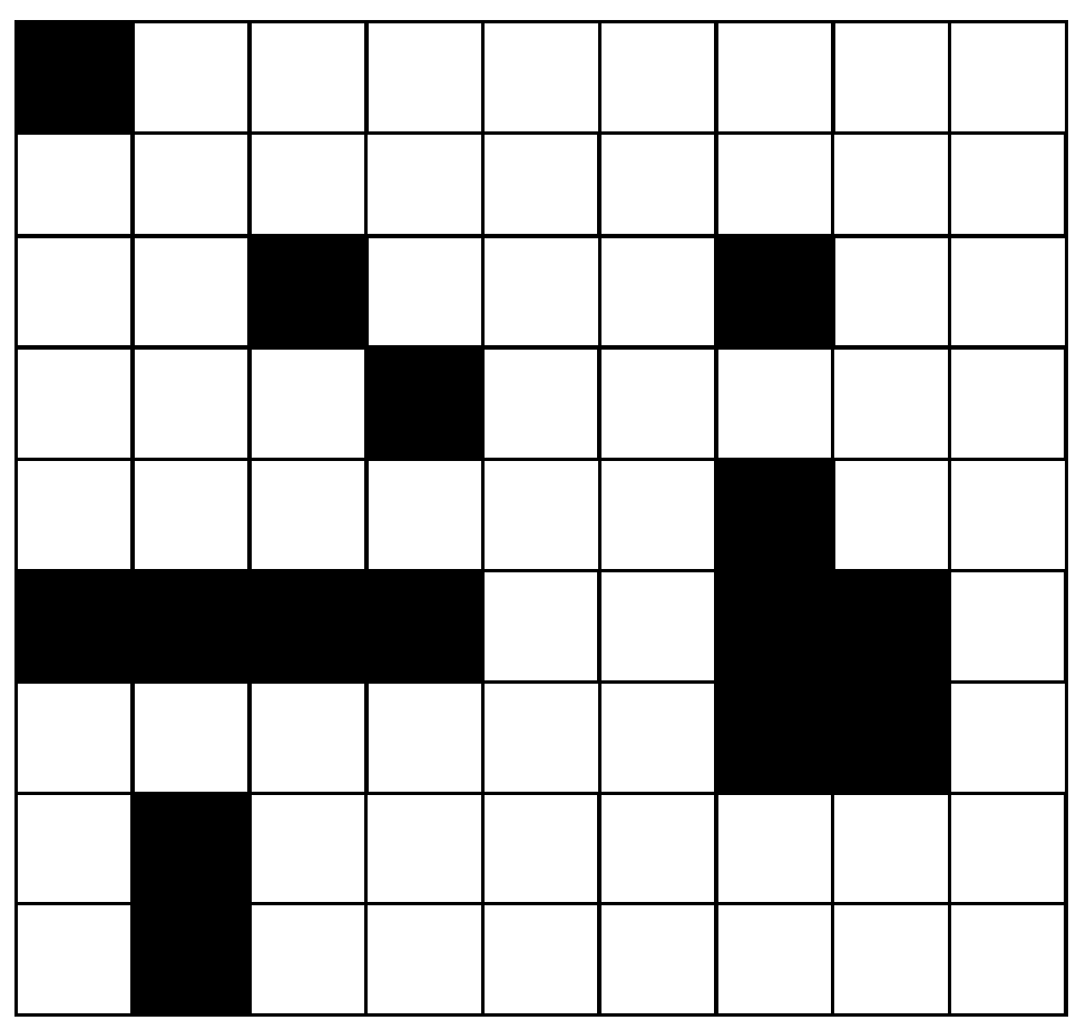
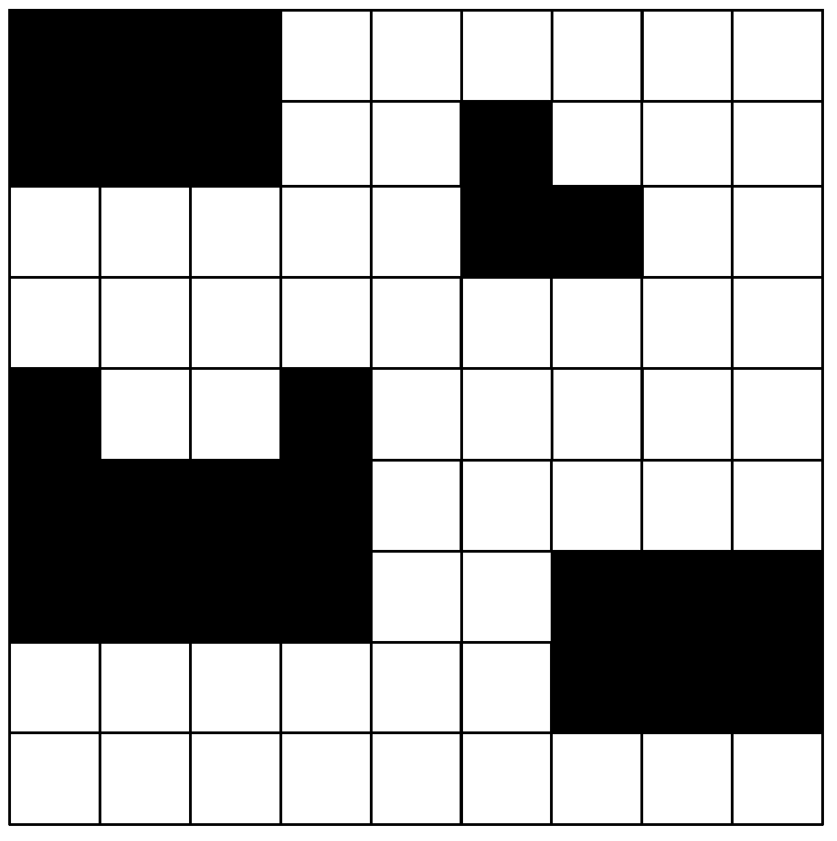
where R represents the mathematical model of a m-row by n-column grid map, rij represents the grid cell at the i-th. row and j-th. column, which i ∈ [0, m) and j ∈ [0, n). The value of rij is 0 or 1, that 0 indicates a free grid and 1 represents an obstacle grid. When m = 9, n = 9, and the side length of each square grid is 1, the grid map represented by R is a 9 × 9 square grid map, as illustrated in Figure 1. On this map, white grids represent free spaces and black grids denote obstacles.

Figure 1.
9 × 9 square grid map.
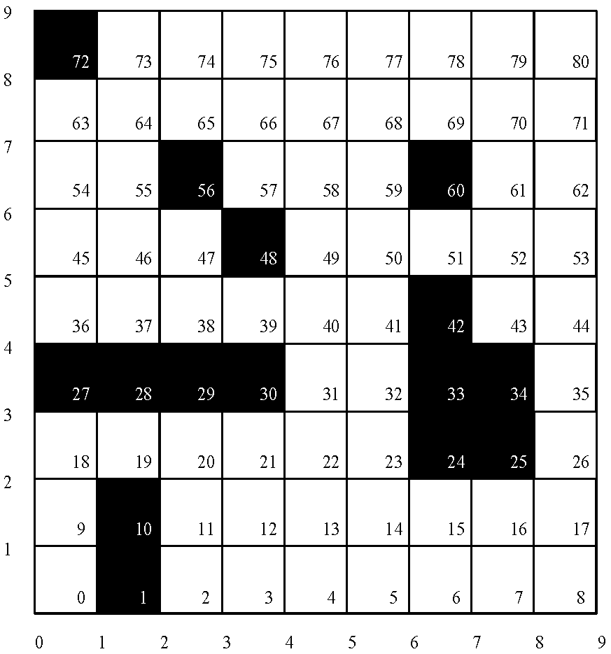
A linear index is introduced for the grid map to enhance the accessibility and processing of grid data and improve pathfinding efficiency. Elements from the 0–1 two-dimensional matrix are mapped into a one-dimensional array in a specific sequence, which reduce memory usage and accelerate access speed. This paper adopts a row-major order principle, which elements of the grid map are mapped into a one-dimensional array starting from the first row and column, proceeding left to right and bottom to top. The linear index begins at 0, and the corresponding calculation formula is provided in Equation (2). This method allows for the rapid location of any element within the grid map without requiring knowledge of its specific row and column positions, as illustrated in Figure 2.
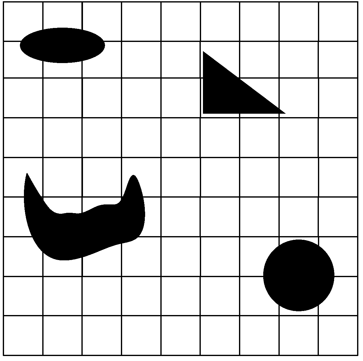
where index (rij) is the linear index of the i-th row and j-th column grid. Because obstacles in real-world environments typically have irregular shapes, the path planning algorithm can be simplified and enhance the computational efficiency by converting these irregular shapes, as illustrated in Figure 3, into regular shapes which are more manageable and computationally tractable. Additionally, grid expansion can be implemented to enhance safety margins. This paper proposes converting each grid cell occupied by an irregularly shaped obstacle into an obstacle grid in its entirety. Even if only a small portion of the grid cell is occupied, the entire cell is designated as an obstacle grid, as illustrated in Figure 4. This approach ensures effective prevention of potential collisions between the robot and obstacles during operation.

Figure 2.
Grid map after building linear indexes.

Figure 3.
Grid maps with irregular obstacle shape.

Figure 4.
Regularized and expanded grid map.
In the context of grid maps, the concepts of grid and node are closely related, with a grid typically representing a node. The attributes of the grid dictate the node’s accessibility, while the node’s connectivity influences the direction and extent of the path planning algorithm. Thus, the grid and node exhibit a one-to-one correspondence, marked by interdependence and inseparability. Within the grid map, the robot is restricted to movement within the node areas designated as free grids, and entry into node areas marked as obstacle grids is prohibited. This paper stipulates that path planning computations are based on the coordinates of each grid’s center position. However, since robot movement in this study is not confined to the cardinal directions (up, down, left, and right), there may be instances where the planned path intersects the vertices of the square grids, as illustrated in scenarios a and b in Figure 5. This paper regularizes and expands irregularly shaped obstacles within the grid map. Consequently, scene (a) represents a scenario where the robot can traverse normally without collision, whereas scene (b) indicates a planned path that intersects obstacles. This latter scenario must be avoided in subsequent path planning to ensure effective navigation.
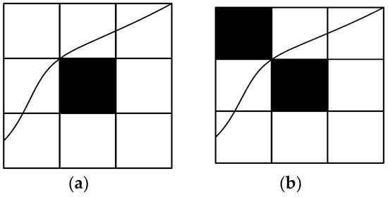
Figure 5.
Planning paths through square grid vertices. (a) Scenario 1. (b) Scenario 2.
3. Traditional A* Algorithm
The A* search algorithm is a highly effective heuristic method commonly employed in robotic path planning. It integrates the features of breadth-first search with greedy-first search, which assesses the merits and demerits of various paths through an evaluation function, thereby enhancing search efficiency. The preliminary A* Algorithm operates on the principle of continuously managing two lists: the openList, which contains pending nodes, and the closedList, which includes processed nodes. Nodes with the lowest evaluated function value are cyclically transferred from the openList to the closedList until the target node is located. If the openList is depleted or the target node remains unfounded, the search is deemed unsuccessful [14]. The evaluation function for the A* algorithm is illustrated in Equation (3):
where g(n) represents the cumulative cost function of the path from the start node to the current node n, h(n) represents the heuristic function estimating the cost of the optimal path from the current node n to the target node, and f(n) is the integrated cost function. This function must be continually evaluated to select the next optimal node and minimize the total cost. In extreme cases where the heuristic function h(n) is significantly smaller than g(n) or even zero, the evaluation function f(n) is predominantly determined by g(n). Consequently, the A* algorithm progressively approximates Dijkstra’s algorithm, which result in a path search that involves traversing more nodes. Increasing node traversal leads to reduce search efficiency; but it generally still ensures the identification of the optimal path. Conversely, when the heuristic function h(n) greatly exceeds g(n), the evaluation function f(n) is primarily influenced by h(n). In this scenario, the A* search effectively transforms into a best-first search, which leads to faster search efficiency, however the paths found may not be optimal. This illustrates that the choice of heuristic function h(n) significantly impacts algorithm performance, because different heuristics can yield varied search outcomes. There are three most commonly utilized distance metrics in heuristic functions, which include Manhattan distance, Euclidean distance, and diagonal distance, as illustrated in Figure 6.
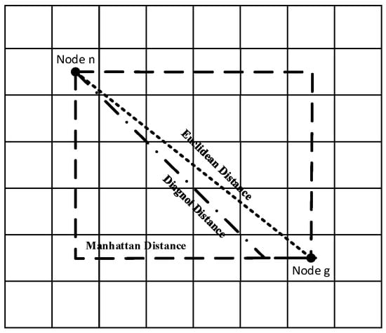
Figure 6.
Three common distance algorithms.
The Manhattan distance, within the conventional Cartesian coordinate system, is defined as the sum of the absolute differences between the x-coordinates and y-coordinates of the current node and the target node [15]. This metric, detailed in Equation (4), signifies that movement occurs exclusively along horizontal or vertical axes, disregarding any diagonal displacement.
The Euclidean distance represents the straight-line distance between the current node and the target node, as defined in Equation (5) [16]. However, in grid-based maps, where movement is restricted to horizontal and vertical directions along the grid, the Euclidean distance is usually not the best choice.
The Diagonal distance represents the maximum number of steps required to move from the current node to the target node in any direction [17], including diagonals. Its formal expression is provided in Equation (6).
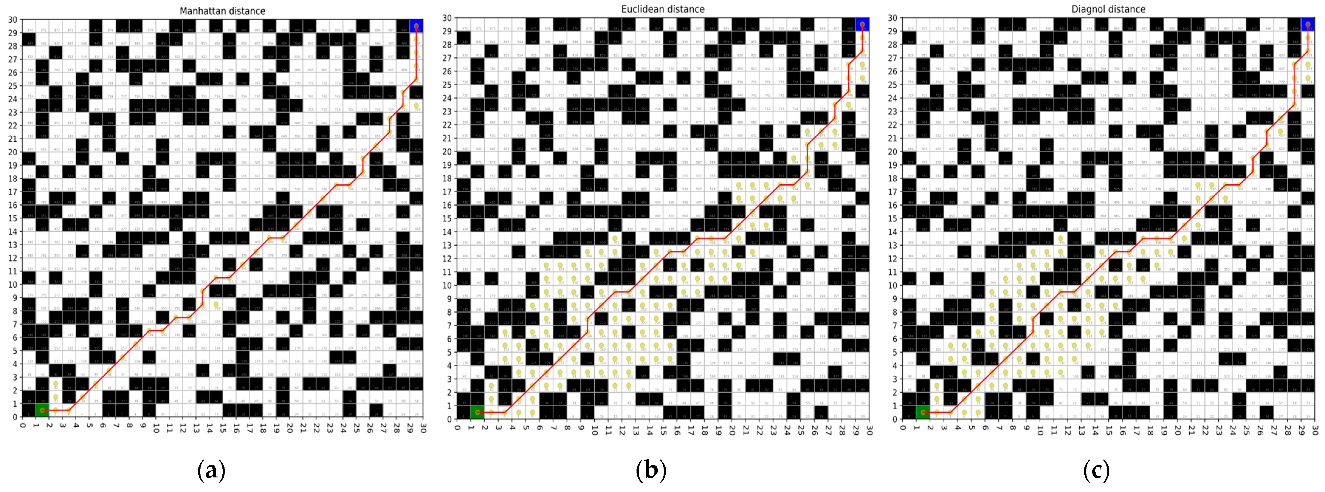
where, g.x, g.y represents the horizontal and vertical coordinates of the target node, and n.x, n.y represents the horizontal and vertical coordinates of the current node. The Manhattan distance directly quantifies the minimum number of steps which are required to traverse from one point to another within grid maps. As a result, Manhattan distance makes it both intuitive and effective for grid-based environments. Compared with the Euclidean distance and Diagonal distance, the computation of the Manhattan distance involves only addition and absolute value operation, excluding square root calculations. This results in greater efficiency and adaptability. This study evaluates the three distance metrics within a grid map of size 50 × 50 and an obstacle density of approximately 35%, as illustrated in Figure 7. The circles in Figure 7 represent the search points. The experimental results, presented in Table 1, demonstrate that the Manhattan distance results in fewer traversal nodes compared with the Euclidean distance and Diagonal distance, in order to enhance search efficiency. Consequently, the Manhattan distance is adopted as the heuristic function for distance in this paper.
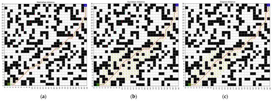
Figure 7.
Simulation results for three distance equations. (a) Manhattan distance. (b) Euclidean distance. (c) Diagonal distance.

Table 1.
Experimental data for three different distance equations.
4. Improved A* Algorithm
4.1. Search Field Optimization
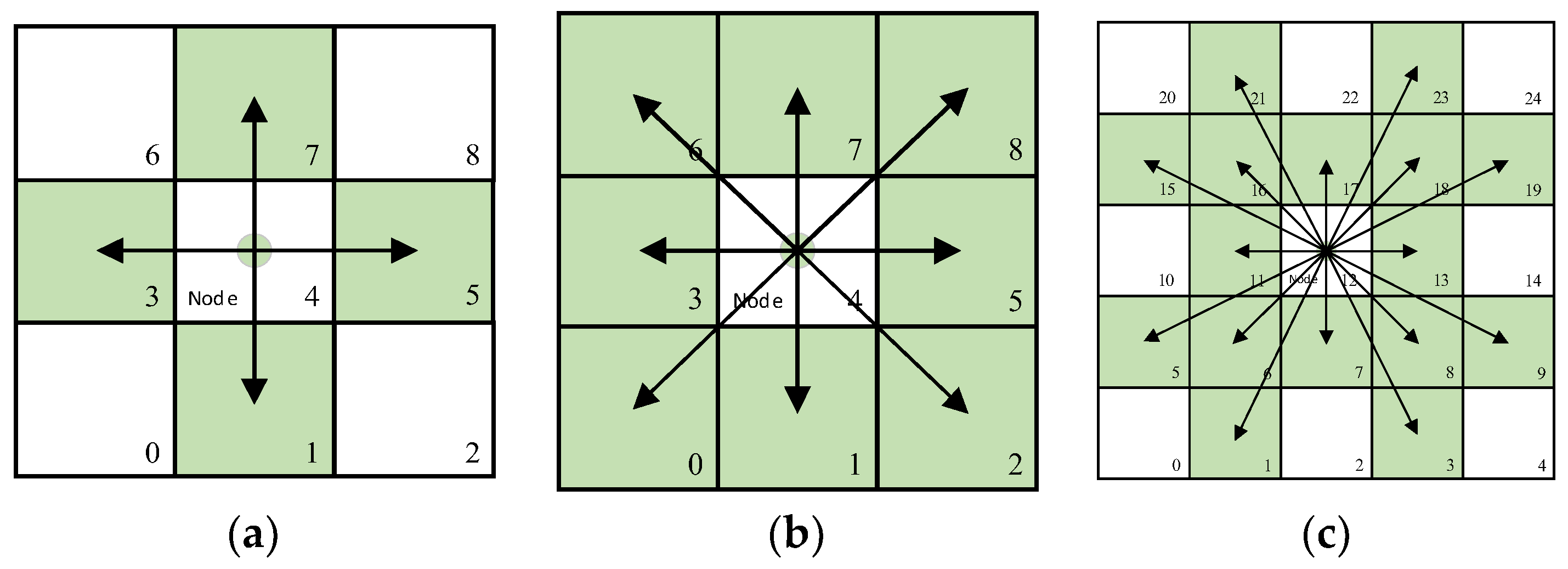
Search neighbor primarily denotes the set of child nodes that are directly reachable when the parent node extends its search. Optimizing the search neighbor is therefore crucial for minimizing computational effort and enhancing the search efficiency of the A* algorithm. The Traditional A* algorithm employs the 8-neighbor, 8-direction search strategy [18,19], which identifies reachable child nodes in the upward, downward, leftward, rightward, and four diagonal directions relative to the current parent node, as depicted in Figure 8b. Optimizing the search neighbor constrains the search range, which is beneficial in scenarios such as grid maps with a high obstacle density or specific movement constraints. For instance, the 8-neighbor, 8-direction search can be refined to a more restricted 4-neighbor, 4-direction search, as illustrated in Figure 8a. This refinement minimizes the number of extraneous search nodes, thereby enhancing algorithm efficiency. Conversely, optimizing the search neighbor can also expand the search range, potentially including 16-neighbor, 32-neighbor, or even 48-neighbor. The 16-neighbor, 16-direction search is depicted in Figure 8a. This expansion enhances the search flexibility, thereby facilitating the identification of more optimal paths.
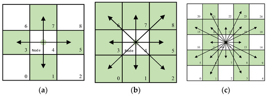
Figure 8.
Search neighbor. (a) 4-Neighbor 4-Direction. (b) 8-Neighbor 8-Direction. (c) 16-Neighbor 16-Direction.
To reconcile flexibility and execution efficiency in A* algorithm, this study introduces a 16-neighbor, 8-direction search strategy according to the principle of symmetry. This approach builds upon the 16-neighbor, 16-direction framework by selecting child nodes within 90° to the left and right of the line connecting the current parent node to the target node for extended search, while excluding other non-essential child nodes, as illustrated in Figure 9. This method of removing non-essential child nodes is obtained based on symmetry and this approach reduces the number of nodes by half to improve the search time. This strategy enhances the flexibility of the A* algorithm search while simultaneously reducing ineffective search efforts and improving overall search efficiency. Consequently, the optimized A* algorithm can better accommodate environmental changes and exhibit superior overall performance.
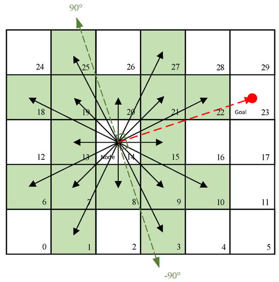
Figure 9.
16-Neighbor 8-Direction schematic.
Given the stochastic nature of obstacle placement, this study evaluates potential obstacle locations. When obstacles are situated among the eight neighbors of the outer layer—represented by nodes 1, 3, 10, 22, 27, 25, 18, and 6 in Figure 9—the directions within the pruning angle range of (−90°, 90°) can be directly pruned. Consequently, the search can proceed unrestrictedly in other directions. If obstacles are located among the eight neighbors of the inner layer—illustrated by nodes 7, 8, 9, 15, 21, 20, 19, and 13 in Figure 9—additional pruning within the (−90°, 90°) angular range is required to prevent obstacle crossing. For instance, in Figure 9, within the (−90°, 90°) angular range relative to the line connecting the current parent node and the target node, the child nodes in the eight directions are nodes 20, 27, 21, 22, 15, 10, 9, and 3. In this scenario, if an obstacle is located at node 15, the directions corresponding to nodes 15, 22, and 10 are pruned. If the obstacle is at node 21, the directions corresponding to nodes 21, 27, and 22 are pruned. Should obstacles be present at both node 15 and node 20, the directions corresponding to nodes 20, 27, 21, 22, 15, and 10 are pruned. Other cases follow a similar pattern. The implementation specifics are determined based on the reachability of the 16 extended sub-nodes, with the corresponding formula provided in (7). This allows for the application of pruning to the eight directions post-selection.
where O(x, y) denotes whether the child node with horizontal and vertical coordinates of x, y is reachable or not, r(x1, y1) is the value of the grid of the child node with horizontal and vertical coordinates of x1, y1, which takes the value of 0 or 1, where 0 denotes a feasible grid and 1 denotes an obstacle grid, and ∆x and ∆y denote the difference in the horizontal and vertical coordinates of the child node and the parent nod.
4.2. Heap Optimization
Given that the A* algorithm requires the continuous management of the pending node list, which referred to as openList, and the processed node list, which referred to as closedList, throughout its execution—particularly in the context of large-scale or complex maps—the time complexity associated with frequent traversals, searches, and sorting operations within openList can escalate to O(n), which impose significant demands on time and computational resources. Consequently, optimizing the data structure of openList is expected to substantially enhance the execution efficiency of the A* algorithm [20]. This paper presents an optimization of openList through the use of a min-heap data structure. In this approach, the node with the smallest f(n) value is always positioned at the top of the heap, which eliminates the need for a global sort of the entire openList and reduces sorting overhead. Consequently, the time complexity for locating nodes is reduced to O(1), while the complexities for insertion and deletion operations are reduced to O(log n). By enhancing node selection efficiency and minimizing unnecessary searches, the algorithm’s overall time complexity is reduced, which leads to significant improvements in both the speed and performance of pathfinding. This is particularly evident in large-scale or complex maps, where the benefits of heap optimization are most pronounced.
4.3. Evaluation Function Optimization
According to the evaluation function Equation (3) of the A* algorithm, the value of f(n) is determined by the cumulative cost function g(n), which represents the path cost from the start node to the current node n, and the heuristic function h(n), which estimates the cost of the optimal path from the current node n to the target node. Typically, g(n) and h(n) are weighted equally with a default ratio of 1:1. However, in many instances, an equal weighting of g(n) and h(n) may result in suboptimal search performance of the A* algorithm [21]. Consequently, during the A* search process, the functions g(n) and h(n) can be appropriately adjusted, or their respective weights can be redistributed to enhance the algorithm’s search efficiency. When the distance between the current node and the target node is considerable, the value of h(n) can be increased to expedite the search by providing more guidance towards the target node. Conversely, if the distance is relatively short, reducing h(n) might slow down the search but prioritize finding the optimal path. Therefore, the evaluation function f(n) in this study fully considers the obstacle rate, the distance relationship of the current node, the positional relationship, and the turn penalty cost, and finally the evaluation function f(n) is obtained as shown in Equation (8):
In summary, this study introduces a dynamic weighting strategy which is designed to enhance the heuristic valuation function. This strategy adjusts the relative importance of g(n) and h(n) by incorporating a weighting function w(n) for h(n) to improve search speed and maintain the relative optimality of the planning path. As detailed in Equation (11), the weighting function w(n) for the heuristic function h(n) is expressed as:
Firstly, the A* algorithm’s performance is closely related to the distance between the current node and the target node. This study considers the relationship between the current node and the target node as well as the start node in order to realize the precise positioning of the current node. This study expresses the relationship between the Euclidean distance from the current node n to the target node g and the Euclidean distance from the start node s to the target node g in Equation (10):
where, g.x, g.y represents the horizontal and vertical coordinates of the target node, s.x, s.y represents the horizontal and vertical coordinates of the start node, and n.x, n.y represents the horizontal and vertical coordinates of the current node.
The search efficiency of the A* algorithm is influenced not only by the distance between the current node and the target node but also by the complexity of the intervening map environment. In the presence of sparse obstacles, the value of h(n) can be increased to improve search efficiency. Conversely, in scenarios with higher complexity and density of obstacle, the value of h(n) can be reduced to prioritize the identification of the optimal path. The variable p represents the number of obstacles between the current node n and the target node g. P(n) represents the probability of the presence of an obstacle in the rectangle formed by the current node n and the goal node g. The obstacle rate in the specified region is expressed as follows:
The A* algorithm should dynamically adapt its search strategy and speed which are based on the relative position of the current search node to the line connecting the start node and the target node. This adjustment ensures the identification of the shortest path while minimizing unnecessary computation time. If the current node is near the line which connects the start node to the target node, it is likely to be on or close to the shortest path. In such case, the search speed should be increased to expedite verification whether the current node is part of the shortest path, and reduce unnecessary searches in regions far from the shortest path. Conversely, when the current node is far from the line, the search speed should be reduced, and the search area should be expanded to ensure the identification of the optimal path. The relative position coefficient of the line connecting the current search node n, the start node s, and the target node g is defined as the ratio of the vector from s to g and the outer product of the vector from n to g with the area of the grid map, as shown in Equation (12):
To effectively minimize turning angles and reduce unnecessary turning points, this study introduces a penalty function t(θ) to account for direction changes within the A* algorithm inspired valuation function. Section 4.1 details that, following the optimization of the search neighbors, there are typically eight directions for the extended search of child nodes. The angle θ = {0, 22.5°, 45°, 67.5°, 90°} represents the angle between each direction and the line connecting the target node to the parent node. The corresponding values of t(θ) are assigned based on the degree of directional change, as illustrated in Equation (13):
4.4. Search Strategy Optimization
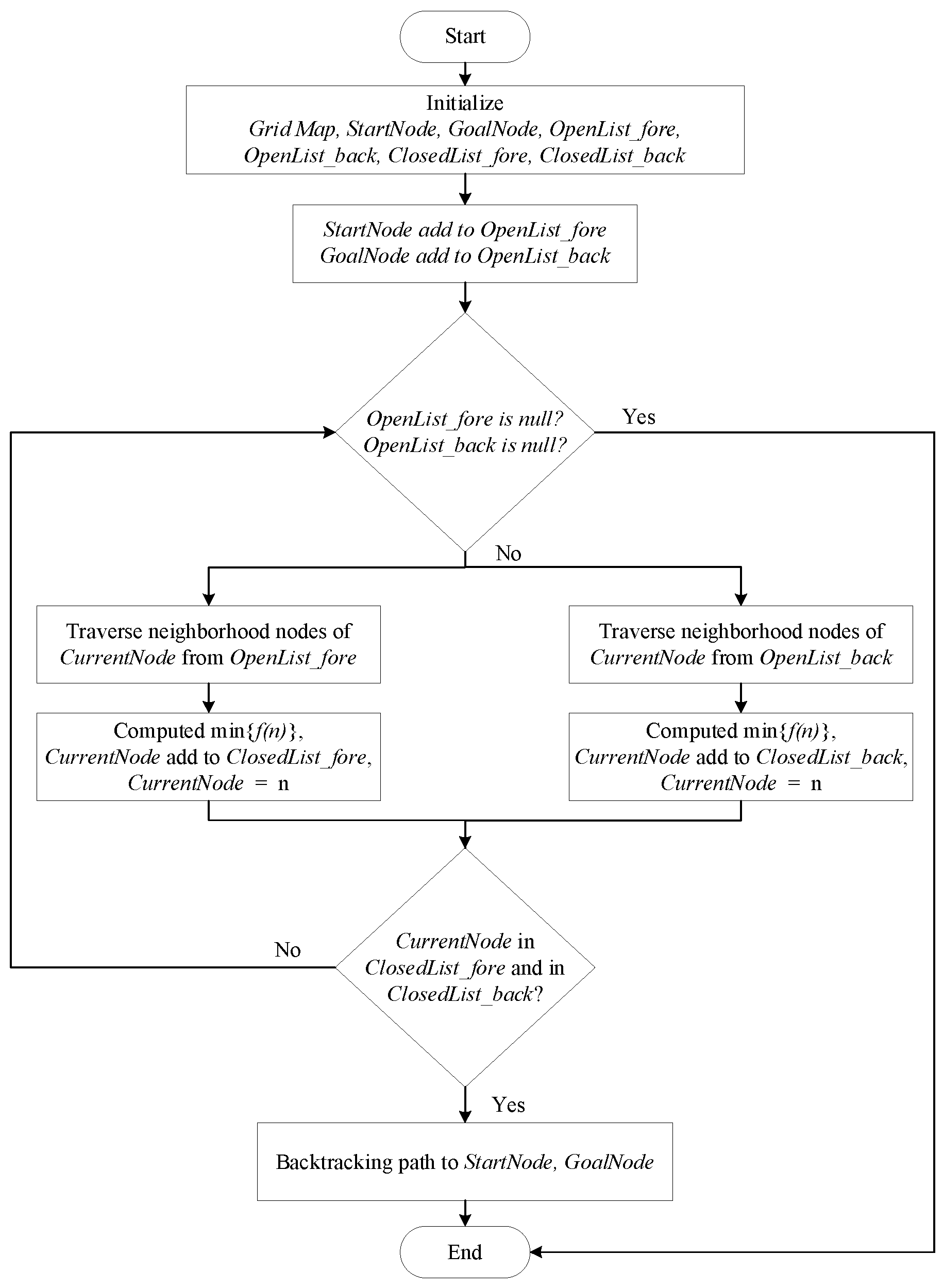
Typically, the A* algorithm initiates at the start node and incrementally searches towards the target node, thereby forming a feasible path. However, this unidirectional search method necessitates traversing numerous nodes, resulting in suboptimal search efficiency. To substantially enhance the overall search efficiency of the A* algorithm, this study introduces a bidirectional search strategy designed to optimize it [22]. Specifically, the search progresses independently from both the start node and the target node towards each other until their respective paths intersect. This approach not only forms a viable path between the start and target nodes but also accelerates the search speed, reduces the number of nodes explored, and enhances overall search efficiency. The flow of the simplified bidirectional A* algorithm is shown in Figure 10.
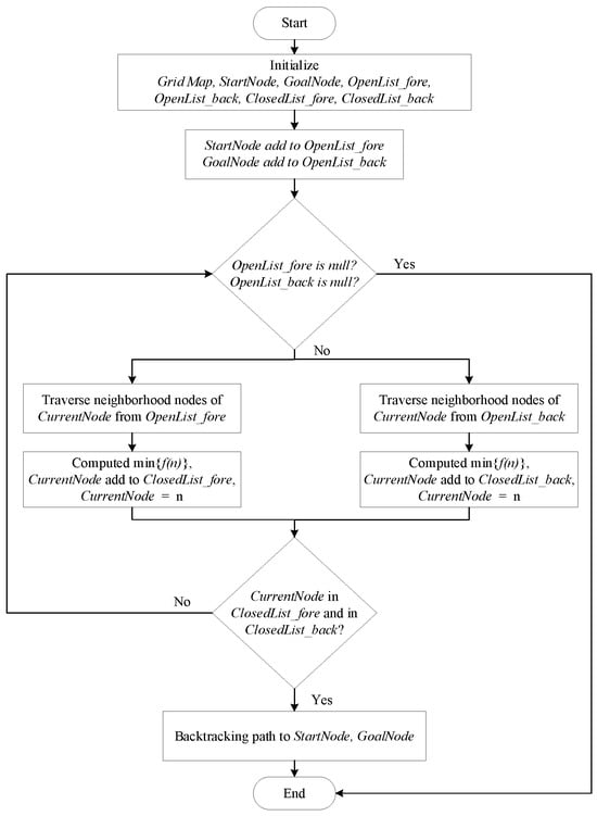
Figure 10.
Bi-directional A* algorithm flowchart.
4.5. Path Optimization
To address the issue of redundant nodes in the planning path, this study introduces a method for identifying co-linear nodes by evaluating whether every set of three consecutive nodes in the path aligns. Furthermore, leveraging the penalty coefficient for directional changes t(θ), as discussed in Section 4.3, allows for the removal of superfluous inflection points, thereby enhancing the smoothness and naturalness of the planned path. The formula for co-linearity assessment is provided in Equation (14):
where (x1, y1) denotes the parent node coordinates of the current node, (x2, y2) denotes the current node coordinates, and (x3, y3) denotes the child node coordinates of the current node.
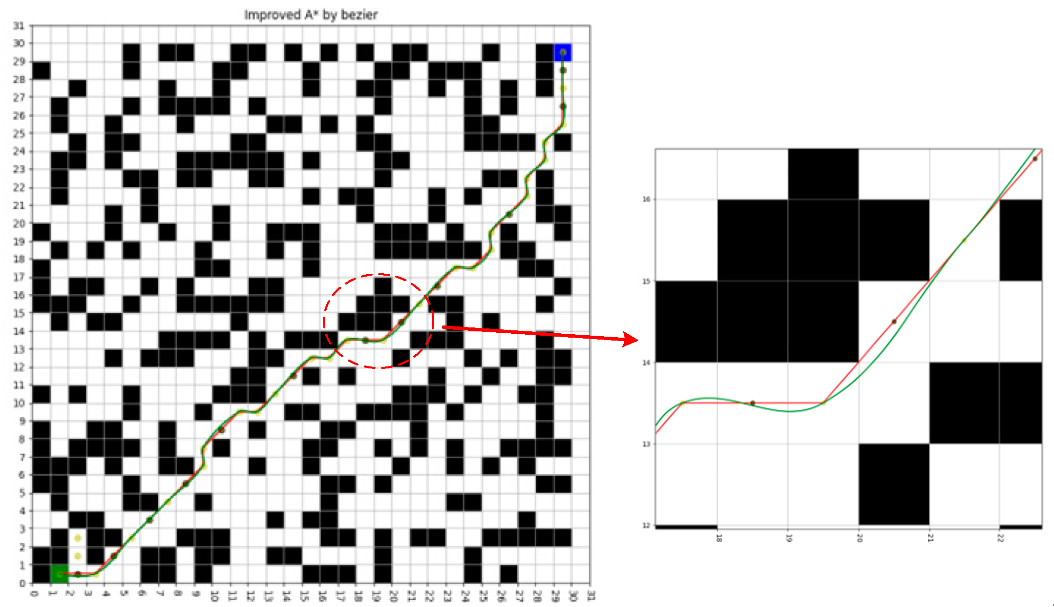
The Bezier curve is a prevalent interpolation method employed for path smoothing in robotic planning, which achieves the desired smoothing effect through a series of control points. As the order of the Bezier curve increases, the resulting curve exhibits greater smoothness; however, this also leads to increased computational complexity and challenges in accurately adjusting control points. Thus, it is essential to balance curve complexity with computational efficiency in practical applications [21]. The cubic bezier curve formulation, detailed in Equation (15), is extensively utilized across diverse research fields due to its inherent flexibility and ease of control. Consequently, this study advocates for the application of the cubic bezier curve to further refine the planned path, adjust nodes appropriately to enhance the smoothness and naturalness of the trajectory, and ultimately develop a navigable path that adheres to the robot’s kinematic constraints, thereby improving the safety of the intelligent mobile robot during practical operations. Figure 11 illustrates the outcome of the planned path on a 30 × 30 grid map following redundant node removal and path smoothing. The red curve represents the original planned path, the green curve denotes the final path processing, yellow dots indicate traversed nodes.
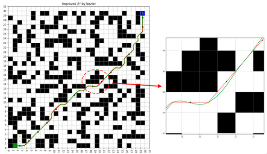
Figure 11.
Path optimization result.
5. Simulation Experiments and Analyses
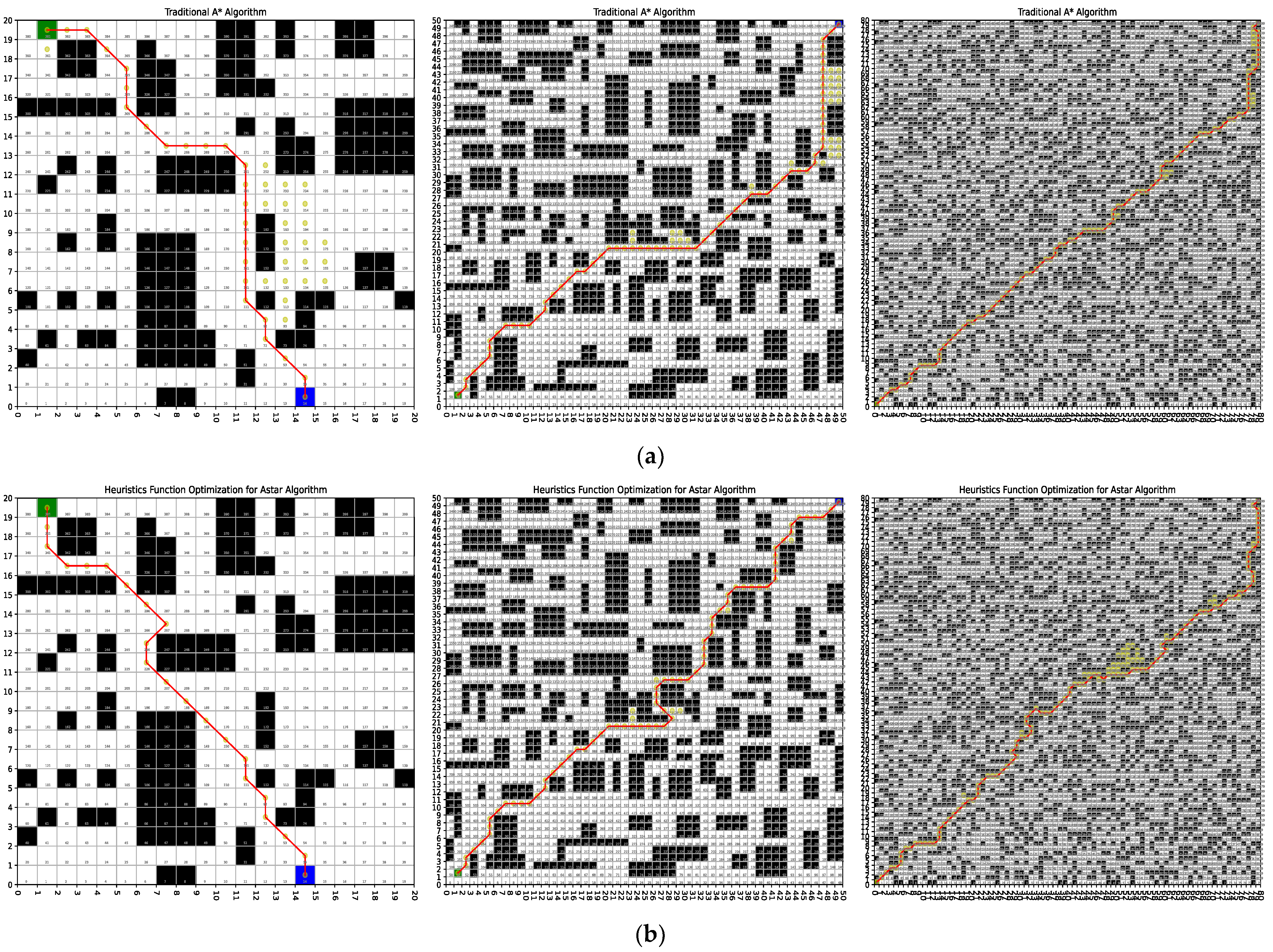
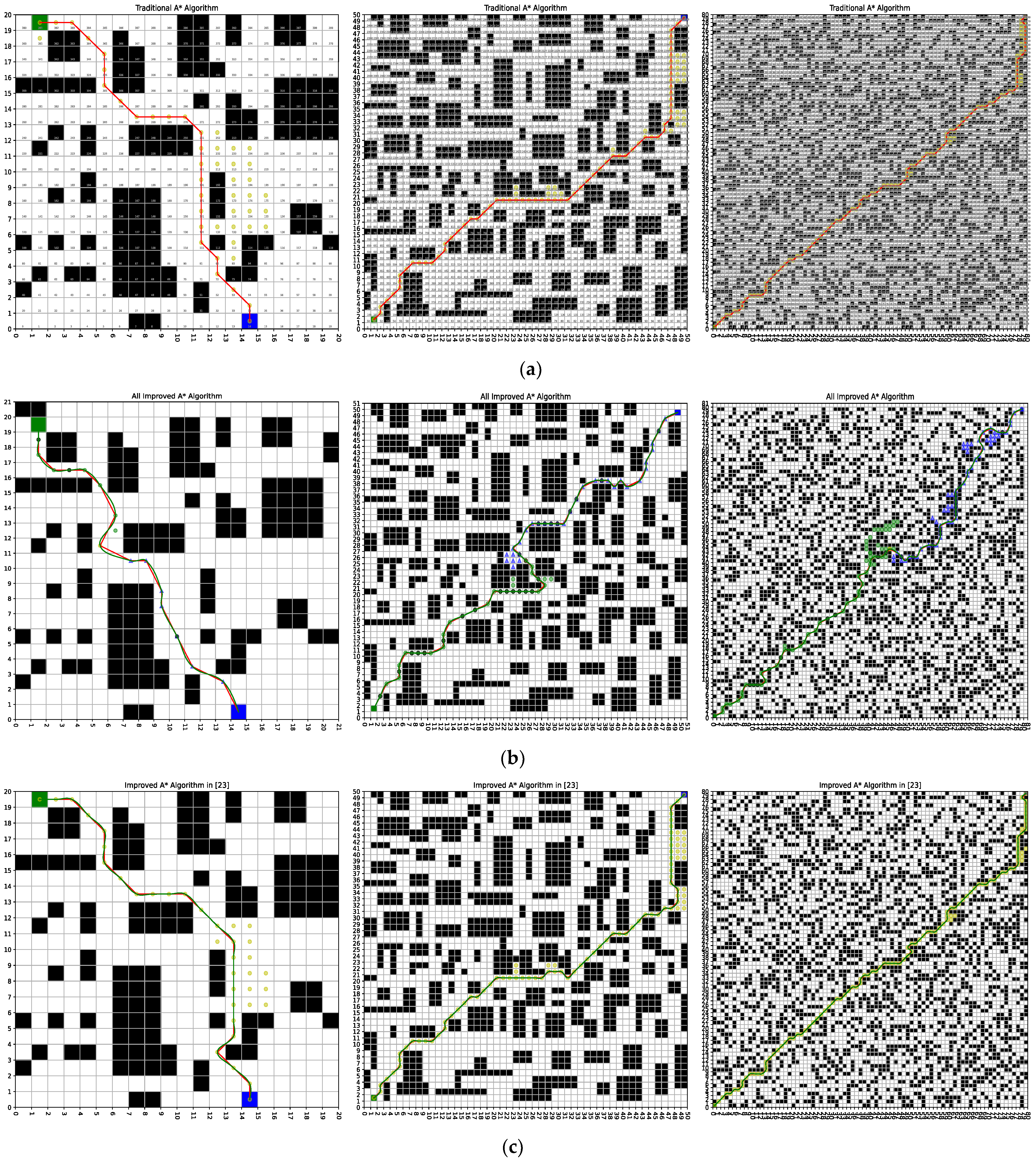
To assess the efficacy of the improved A* algorithm, simulations and comparative experiments were conducted using grid maps of three distinct sizes: 25 × 25, 50 × 50, and 80 × 80. These experiments compared the performance of the traditional A* algorithm with the improved A* algorithm. In Figure 12, Figure 13, Figure 14, Figure 15 and Figure 16, the x-axis starts at 0 from left to right, and the maximum value is the number of grids on the x-axis of the grid map, and the y-axis starts at 0 from bottom to top, and the maximum value is the number of grids on the y-axis of the grid map. The green grid represents the starting point and the blue grid represents the end point.
5.1. Search Field Optimization Experiment
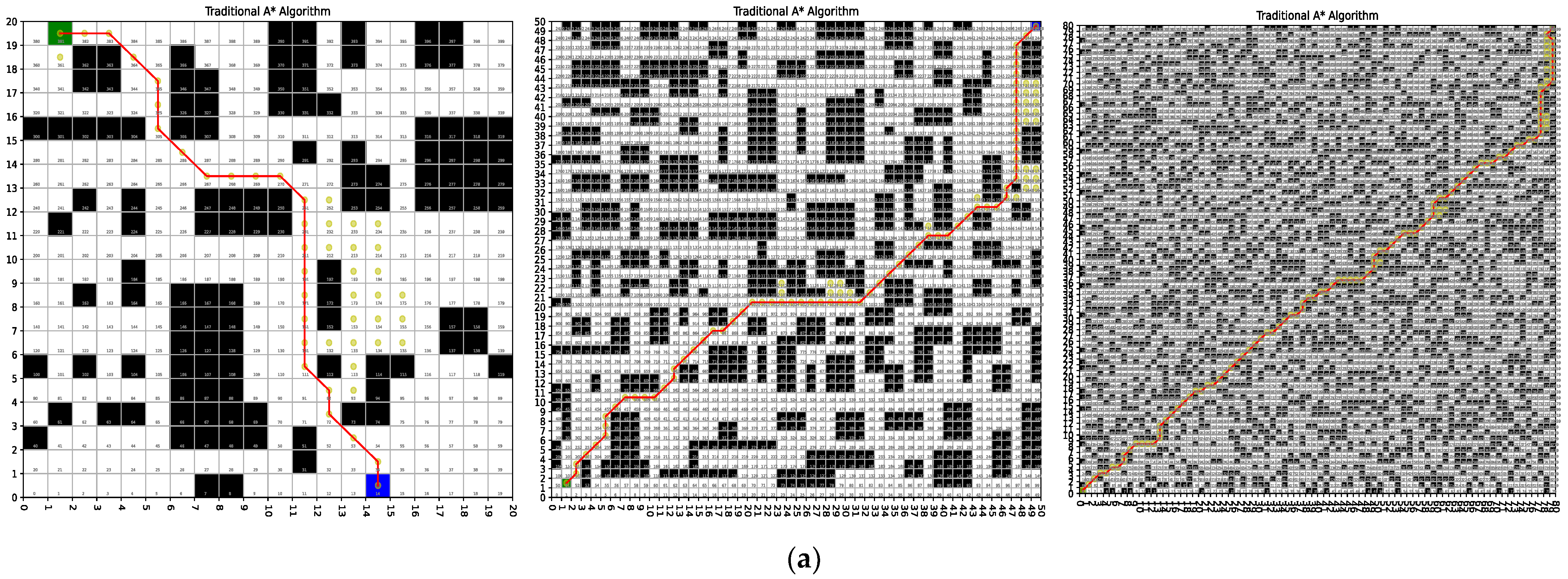
This section aims to evaluate the efficacy of the A* algorithm with search neighbor optimization. The results of these simulation experiments are illustrated in Figure 12 and Table 2. As shown in Table 2, the search neighbor-optimized A* algorithm reduces the search time by 44.8%, the number of traversed nodes by 50%, the final path length by 4.5%, and the number of final path nodes by 28% on the 20 × 20 map, compared to the traditional A* algorithm. On the 50 × 50 map, the search time decreased by 38.9%, the number of traversed nodes increased by 2.1%, the final path length increased by 0.6%, and the number of final path nodes decreased by 19.1%. On the 80 × 80 map, the search time decreased by 18.9%, the number of traversed nodes increased by 5.1%, the final path length increased by 1.7%, and the number of final path nodes decreased by 19.2%. The experimental results demonstrate that the A* algorithm with search neighbor optimization, while not exceptional in terms of the number of traversal nodes, final path length, or number of inflection points, significantly reduces search time, enhances search efficiency, and decreases the number of nodes in the final path. However, the improvement in search efficiency diminishes with the increasing size of the grid map.
Table 2.
Neighbor optimization simulation data.
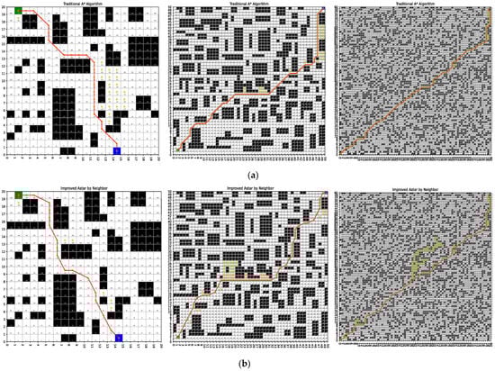
Figure 12.
Neighbor optimization simulation results. (a) Traditional A* algorithm. (b) Neighbor optimized A* algorithm.
Figure 12.
Neighbor optimization simulation results. (a) Traditional A* algorithm. (b) Neighbor optimized A* algorithm.
5.2. Heap Optimization Experiment
This section aims to evaluate the effectiveness of the A* algorithm following heap optimization with a minimal heap. The results of these simulation experiments are illustrated in Figure 13 and Table 3. Table 3 shows that the heap-optimized A* algorithm reduces search time by 20.4%, increases the number of traversed nodes by 21.7%, decreases the final path length by 4.3%, and reduces the number of final path nodes by 8% on the 20 × 20 map compared to the traditional A* algorithm. On the 50 × 50 map, search time decreased by 37.8%, the number of traversed nodes decreased by 2.1%, the final path length decreased by 7.3%, and the number of final path nodes decreased by 1.5%. On the 80 × 80 map, search time is reduced by 16.9%, the number of traversed nodes is increased by 0.8%, the final path length is reduced by 2.3%, and the number of final path nodes is reduced by 4.8%. The experimental results indicate that optimizing the data structure for traversal node storage using a minimal heap effectively reduces search time and enhances search efficiency. Additionally, it positively impacts the reduction in both the number and length of final path nodes.
Table 3.
Heap optimization simulation data.
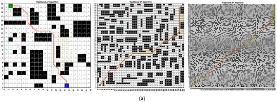
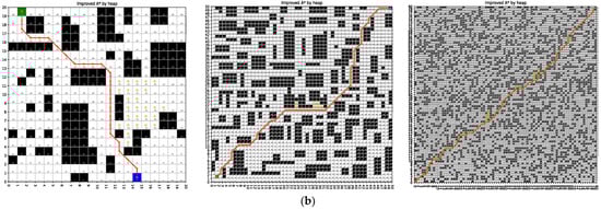
Figure 13.
Heap optimization simulation results. (a) Traditional A* algorithm. (b) Heap optimized A* algorithm.
Figure 13.
Heap optimization simulation results. (a) Traditional A* algorithm. (b) Heap optimized A* algorithm.
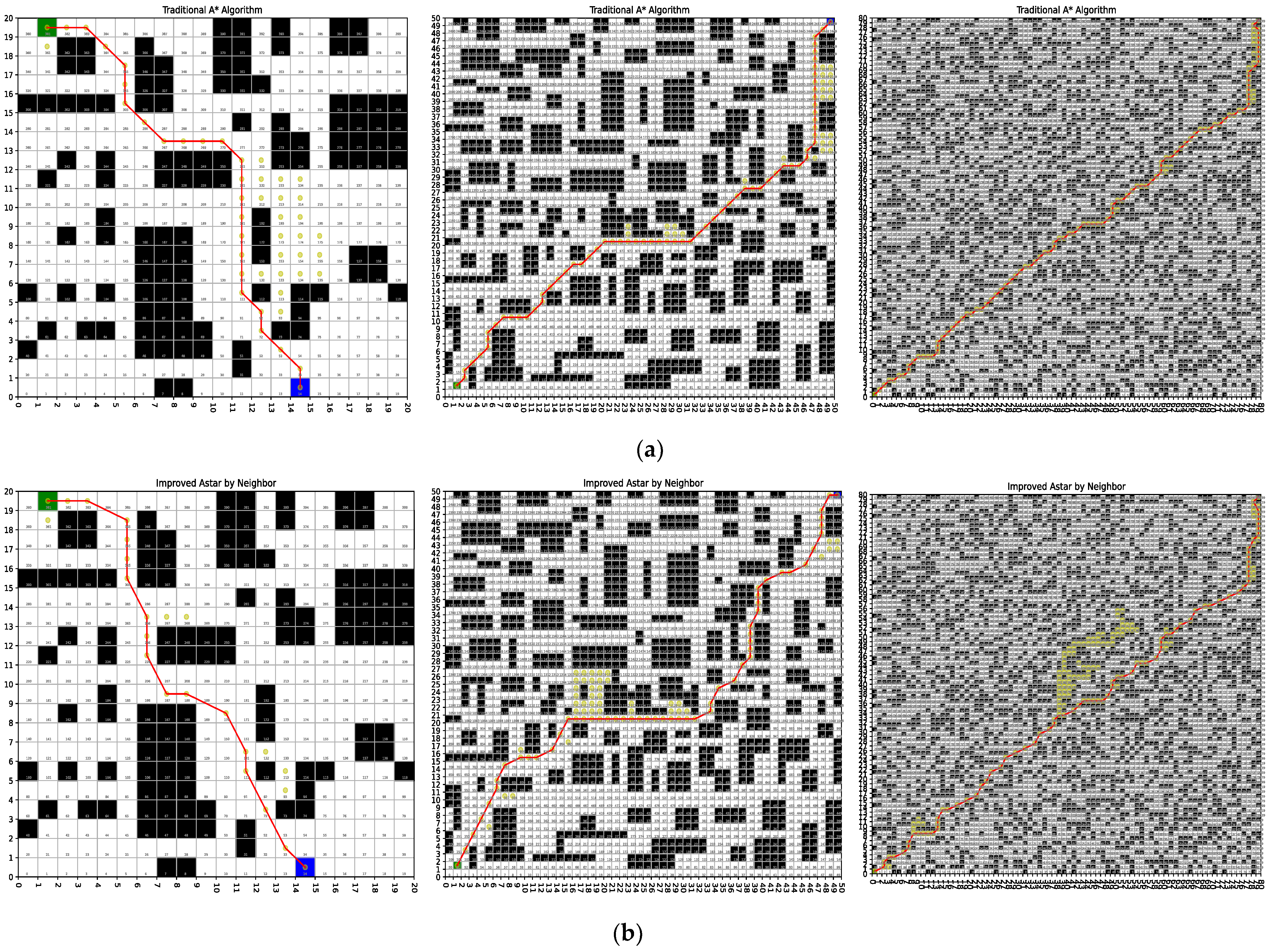
5.3. Bi-Directional Search Experiment
This section aims to assess the effectiveness of the A* algorithm following the optimization of the bidirectional search strategy. The results are presented in Figure 14 and Table 4. To display the A* search paths in both forward and reverse directions, the figure uses green circles to represent the traversal nodes of the forward A* search and blue triangles for the reverse A* search nodes. The meeting points of positive and negative paths are marked with yellow circles, while the planning paths are depicted in red.
Table 4.
Bidirectional search simulation data.
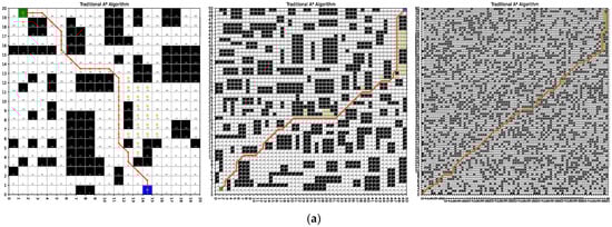
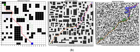
Figure 14.
Bidirectional search simulation results. (a) Traditional A* algorithm. (b) Bidirectional A* algorithm.
Figure 14.
Bidirectional search simulation results. (a) Traditional A* algorithm. (b) Bidirectional A* algorithm.
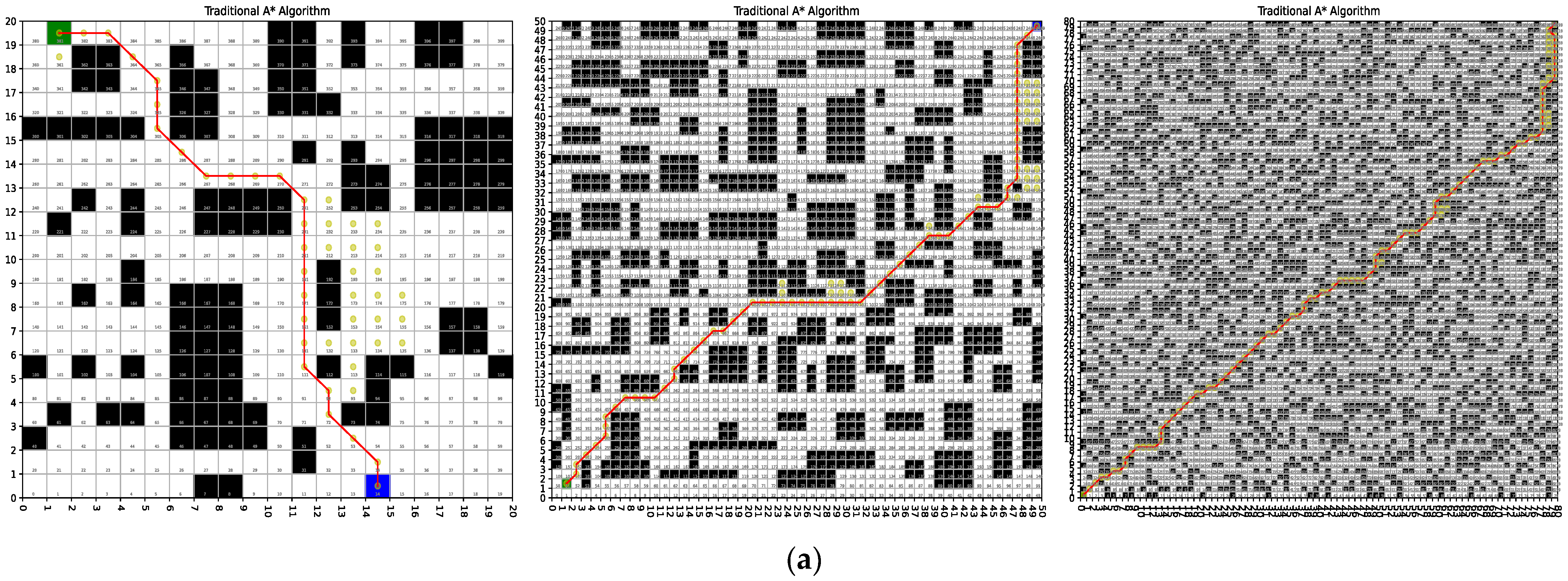
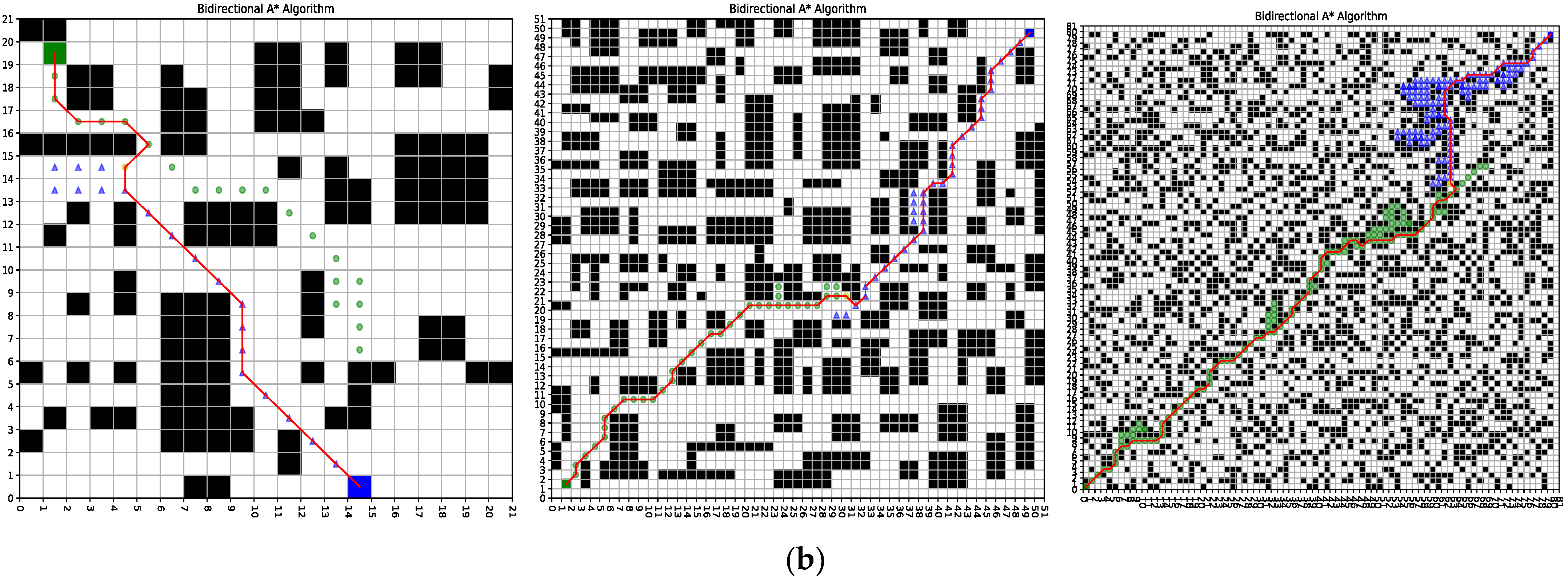
Table 4 illustrates that the optimized A* algorithm, incorporating a bidirectional search strategy, achieves a 72.8% reduction in search time, a 10.8% decrease in the number of traversed nodes, a 4.2% reduction in final path lengths, a 12% decrease in the number of final path nodes, and a 20% reduction in final path inflections on a 20 × 20 map, compared to the traditional A* algorithm. On the 50 × 50 map, the search time decreased by 90.8%, the number of traversal nodes decreased by 20.4%, the length of the final path increased by 9.6%, the number of path nodes decreased by 4.4%, and the number of final path inflection points increased by 35%. On the 80 × 80 map, the search time decreased by 77.4%, the number of traversed nodes increased by 112.7%, the length of the final path increased by 21.7%, the number of final path nodes increased by 8.6%, and the number of final path inflection points increased by 6.1%. The experimental results indicate that while the optimization of the bidirectional search strategy may lead to an increase in the number of traversal nodes and the length of the final path, it significantly enhances the search efficiency of the A* algorithm and substantially reduces search time.
5.4. Evaluation Function Optimization Experiment
This section aims to assess the effectiveness of the A* algorithm following the optimization of the evaluation function. The results of these simulation experiments are presented in Figure 15 and Table 5. Table 5 reveals that the optimized A* algorithm, utilizing a heuristic valuation function, decreases search time by 59.1%, reduces the number of traversed nodes by 52.1%, shortens the final path length by 3.4%, lowers the number of final path nodes by 12%, and increases the number of final path inflection points by 10% on a 20 × 20 map compared to the traditional A* algorithm. On the 50 × 50 map, search time decreased by 44.2%, the number of traversal nodes decreased by 18.2%, the length of the final path increased by 3.5%, the number of final path nodes increased by 2.9%, and the number of final path inflection points increased by 55%. On the 80 × 80 map, search time decreased by 16.9%, the number of traversal nodes increased by 20.3%, the length of the final path increased by 7.6%, the number of final path nodes increased by 7.6%, and the number of final path inflection points increased by 20.4%. The experimental results demonstrate that the enhanced evaluation function, which takes into account the complexity and obstacle density of the grid map, effectively balances search efficiency with optimal pathfinding. This function significantly reduces search time and improves overall search efficiency, thereby ensuring that the planned paths offer both high efficiency and reliability, making them suitable for a broader range of scenarios.
Table 5.
Evaluation function optimization simulation data.
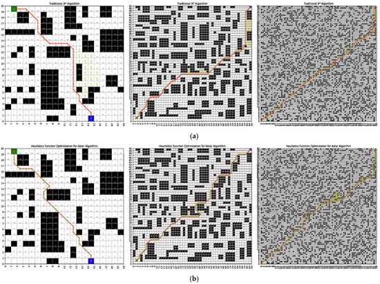
Figure 15.
Evaluation function optimization simulation results. (a) Traditional A* algorithm. (b) Evaluation function optimized A* algorithm.
Figure 15.
Evaluation function optimization simulation results. (a) Traditional A* algorithm. (b) Evaluation function optimized A* algorithm.
5.5. Integrated Experiment
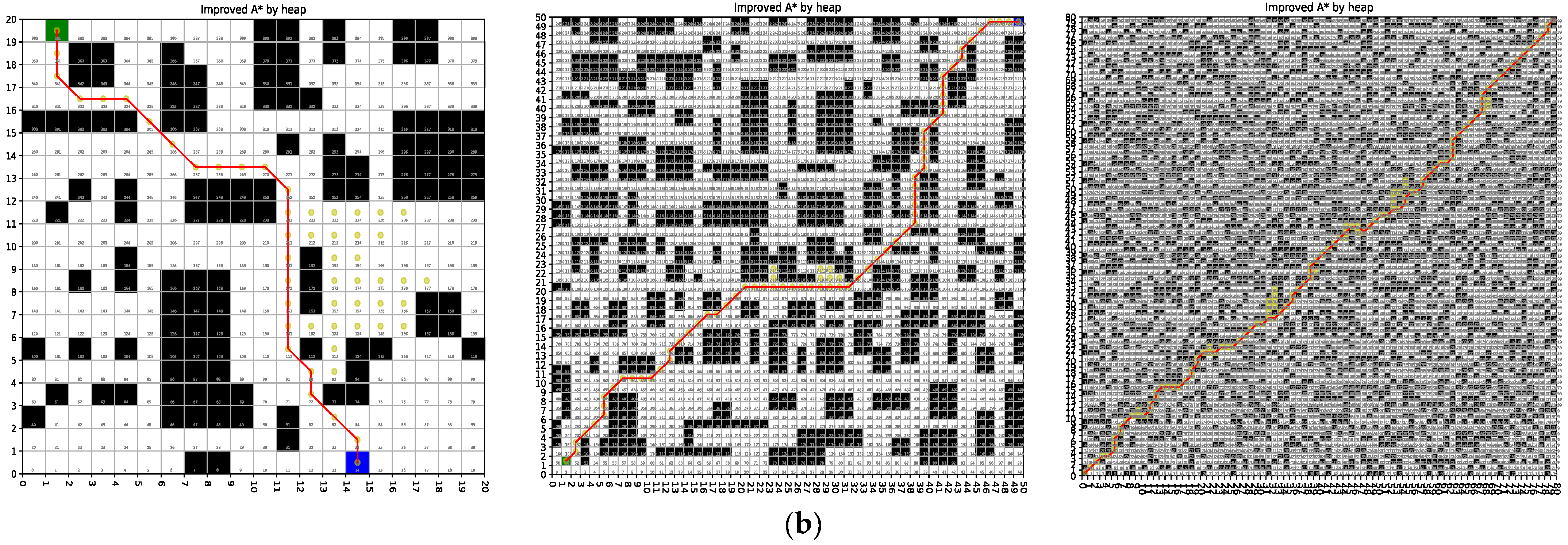
This section aims to evaluate the effectiveness of the A* algorithm following the integration of all previously discussed optimizations. The results of these simulation experiments are illustrated in Figure 16 and Table 6. Table 6 demonstrates that the improved A* algorithm decreases search time by 99.1%, reduces the number of traversed nodes by 63%, shortens the final path length by 26.3%, lowers the number of final path nodes by 32%, and reduces the number of final path inflection points by 20% on the 20 × 20 map compared to the traditional A* algorithm. On the 50 × 50 map, search time decreased by 87.2%, the number of traversal nodes decreased by 27.9%, the final path length increased by 55.2%, the number of final path nodes decreased by 14.7%, and the number of final path inflection points increased by 55%. On the 80 × 80 map, search time was reduced by 84.5%, the number of traversal nodes increased by 14.4%, the final path length increased by 73.5%, the number of final path nodes decreased by 18.2%, and the number of final path inflection points increased by 22.4%. The simulation experiments indicate that the improved A* algorithm significantly improves search time and consequently boosts search efficiency. However, improvements in the number of traversal nodes, path length, and other metrics are less pronounced. Analysis suggests that this phenomenon is primarily due to changes in the search strategy following modifications to the evaluation function, which involved setting the weight function of the heuristic and introducing a turn penalty function. These adjustments affected the weight coefficients of the nodes, thereby increasing the computational cost associated with path length. Additionally, for large grid maps, the bidirectional search strategy, which initiates searches from both the start and target nodes simultaneously, can lead to variations in the selection of the relative optimal path. This often results in an increased number of traversal nodes. Despite the addition of a turn penalty function to the evaluation criteria to minimize unnecessary turns, the optimization of search neighbor, the bidirectional search strategy, and the weight function settings have rendered the improved A* algorithm less effective in reducing the number of path inflection points. Compared with the improved A* algorithm proposed in literature [21], it can be obtained from Table 6 that the improved A* algorithm proposed in this paper still has a large advantage in search time. Although the search path increases, the algorithm proposed in this paper avoids regions with more obstacles to achieve high security. Figure 16 illustrates that the application of the path redundant node elimination mechanism and the optimization of the cubic bezier curve result in a smoothed path, depicted as the green folded line. This enhanced path is better suited for robot movement, thereby improving the safety of the planned trajectory and aligning more closely with the robot’s operational requirements. In summary, the comparative results demonstrate that the improved A* algorithm proposed in this study exhibits superior overall performance, significant effectiveness, and robustness, making it applicable to a variety of scenarios.
Table 6.
Improved A* Algorithm simulation data.
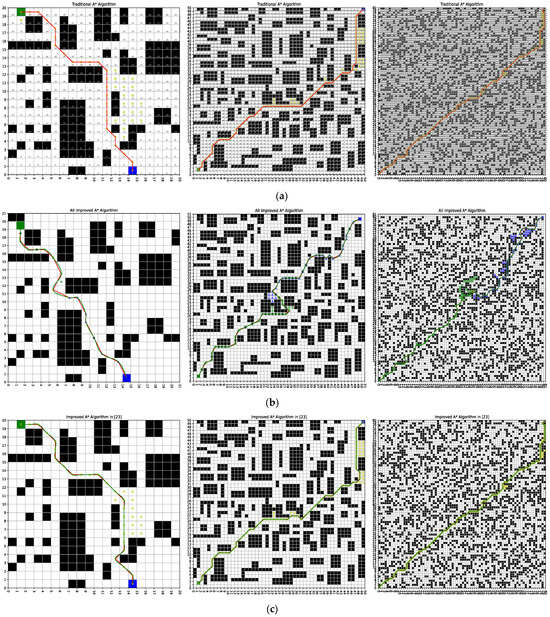
Figure 16.
Improved A* Algorithm simulation results. (a) Traditional A* algorithm. (b) Improved A* algorithm. (c) The improved A* algorithm proposed in the literature [23].
Figure 16.
Improved A* Algorithm simulation results. (a) Traditional A* algorithm. (b) Improved A* algorithm. (c) The improved A* algorithm proposed in the literature [23].
6. Conclusions
This study focuses on intelligent mobile robots, specifically addressing the limitations of traditional A* pathfinding algorithms, such as excessive node traversal, low search efficiency, and poor adaptability across diverse environments. To overcome these challenges, an improved A* algorithm is proposed for the path planning of intelligent mobile robots. Comparative experiments conducted across various grid map sizes demonstrate that this improved A* algorithm exhibits superior effectiveness and robustness. The key improvements introduced in the A* algorithm in this study are primarily as follows:
- The proposed optimization refines the A* algorithm by upgrading the search neighbor model from an 8-neighbor, 8-direction framework to a 16-neighbor, 8-direction framework. This enhancement leverages the positional relationship between the current node and the target node during the search process, thereby improving both the directionality and efficiency of the A* algorithm’s search.
- The optimization of the storage structure of traversed nodes using a minimum heap significantly decreases the time complexity associated with node traversal, thereby reducing the overall search time.
- An adaptive weight function is designed based on the complexity of the grid map, the obstacle density, and the positional relationship between the current node and the line connecting the start and target nodes. This function optimizes the evaluation process by balancing search efficiency and path optimality, thereby enhancing the overall performance of the A* algorithm. It allows the algorithm to adapt to a broader range of scenarios while maximizing both search efficiency and accuracy.
- The A* algorithm is optimized by transitioning from a unidirectional to a bidirectional search strategy, wherein paths are explored simultaneously from both the start and target nodes. This approach substantially enhances search efficiency, although it may result in a longer final path.
- Inflection points in the planned path are minimized by implementing a turn penalty function, while co-linear redundant nodes are eliminated through a path redundancy rejection mechanism. Additionally, the planned path is smoothed using the cubic Bezier curve, resulting in a trajectory that better meets the robot’s practical requirements.
When compared to the traditional A* algorithm, the improved A* algorithm proposed in this study demonstrates notable improvements in search time, although the impact on node traversal and performance across various grid sizes is less consistent. Future research will focus on further optimizing this improved A* algorithm to improve performance in terms of both search efficiency and node traversal. The improved algorithm proposed in this paper still lacks in terms of path length and number of traversal points, despite the large improvement in time. In future work, we will improve our proposed A* algorithm with novel criteria to reduce searching nodes, accelerate the search process and optimize the calculation time. Additionally, the current study does not address dynamic obstacles in real-world applications. We may apply the path planning method with the Dynamic Windows Algorithm and emphasize real-time path planning to augment the practical applicability of the method.
Author Contributions
Data curation, Q.L.; Formal analysis, Q.L.; Funding acquisition, J.Y.; Methodology, D.W.; Project administration, D.H.; Resources, J.Y.; Supervision, D.H.; Validation, Q.L.; Writing—original draft, D.W.; Writing—review & editing, D.W. All authors will be informed about each step of manuscript processing including submission, revision, revision reminder, etc. via emails from our system or assigned Assistant Editor. All authors have read and agreed to the published version of the manuscript.
Funding
This research was funded by Shanghai Sailing Program, grant number 21YF1400500.
Data Availability Statement
The original contributions presented in the study are included in the article, further inquiries can be directed to the corresponding authors.
Conflicts of Interest
The authors declare no conflicts of interest.
References
- Qin, H.; Shao, S.; Wang, T.; Yu, X.; Jiang, Y.; Cao, Z. Review of autonomous path planning algorithms for mobile robots. Drones 2023, 7, 211–248. [Google Scholar] [CrossRef]
- Zheng, L.; Yu, W.; Li, G.; Qin, G.; Luo, Y. Particle swarm algorithm path-planning method for mobile robots based on artificial potential fields. Sensors 2023, 23, 6082–6097. [Google Scholar] [CrossRef] [PubMed]
- Kobayashi, M.; Zushi, H.; Nakamura, T. Local path planning: Dynamic window approach with Q-learning considering congestion environments for mobile robot. IEEE Access 2023, 11, 96733–96742. [Google Scholar] [CrossRef]
- Zhu, Z.; Yin, Y.; Lyu, H. Automatic collision avoidance algorithm based on route-plan-guided artificial potential field method. Ocean. Eng. 2023, 271, 113737. [Google Scholar] [CrossRef]
- Wang, T.; Li, A.; Guo, D.; Du, G.; He, W. Global Dynamic Path Planning of AGV Based on Fusion of Improved A* Algorithm and Dynamic Window Method. Sensors 2024, 24, 2011. [Google Scholar] [CrossRef]
- Kozhubaev, Y.; Yang, R. Simulation of Dynamic Path Planning of Symmetrical Trajectory of Mobile Robots Based on Improved A* and Artificial Potential Field Fusion for Natural Resource Exploration. Symmetry 2024, 16, 801. [Google Scholar] [CrossRef]
- Chen, Z.; Xiao, J.; Wang, G. An effective path planning of intelligent mobile robot using improved genetic algorithm. Wirel. Commun. Mob. Comput. 2022, 2022, 9590367–9590375. [Google Scholar] [CrossRef]
- Xu, Y.; Li, Q.; Xu, X.; Yang, J.; Chen, Y. Research progress of nature-inspired metaheuristic algorithms in mobile robot path planning. Electronics 2023, 12, 3263–3285. [Google Scholar] [CrossRef]
- Liu, L.; Wang, B.; Xu, H. Research on path-planning algorithm integrating optimization A-star algorithm and artificial potential field method. Electronics 2022, 11, 3660–3681. [Google Scholar] [CrossRef]
- Guo, B.; Kuang, Z.; Guan, J.; Hu, M.; Rao, L.; Sun, X. An improved a-star algorithm for complete coverage path planning of unmanned ships. Inter. J. Pattern Recogn. Art. Intell. 2022, 36, 2259009. [Google Scholar] [CrossRef]
- Zhang, H.; Tao, Y.; Zhu, W. Global path planning of unmanned surface vehicle based on improved A-Star algorithm. Sensors 2023, 23, 6647. [Google Scholar] [CrossRef] [PubMed]
- Liu, C.; Mao, Q.; Chu, X.; Xie, S. An improved A-star algorithm considering water current, traffic separation and berthing for vessel path planning. Appl. Sci. 2019, 9, 1057. [Google Scholar] [CrossRef]
- Gasparetto, A.; Boscariol, P.; Lanzutti, A.; Vidoni, R. Path planning and trajectory planning algorithms: A general overview. In Motion and Operation Planning of Robotic Systems: Background and Practical Approaches; Springer: New York, NY, USA, 2015; pp. 3–27. [Google Scholar]
- Liu, L.; Wang, X.; Yang, X.; Liu, H.; Li, J.; Wang, P. Path planning techniques for mobile robots: Review and prospect. Expert Syst. Appl. 2023, 227, 120254. [Google Scholar] [CrossRef]
- Liu, Y.; Wang, C.; Wu, H.; Wei, Y. Mobile Robot Path Planning Based on Kinematically Constrained A-Star Algorithm and DWA Fusion Algorithm. Mathematics 2023, 11, 4552. [Google Scholar] [CrossRef]
- Chen, G.; Chen, S.; Li, X.; Zhou, P.; Zhou, Z. Optimal seamline detection for orthoimage mosaicking based on DSM and improved JPS algorithm. Remote Sens. 2018, 10, 821. [Google Scholar] [CrossRef]
- Fan, B.; Guo, L. An Improved JPS Algorithm for Global Path Planning of the Seabed Mining Vehicle. Arabian J. Sci. Eng. 2024, 49, 3963–3977. [Google Scholar] [CrossRef]
- Zhang, B.; Zhu, D. A new method on motion planning for mobile robots using jump point search and Bezier curves. Int. J. Adv. Robot. Syst. 2021, 18, 17298814211019220. [Google Scholar] [CrossRef]
- Hu, S.; Tian, S.; Zhao, J.; Shen, R. Path planning of an unmanned surface vessel based on the improved A-Star and dynamic window method. J. Mar. Sci. Eng. 2023, 11, 1060. [Google Scholar] [CrossRef]
- Lu, J.; Zeng, B.; Tang, J.; Lam, T.L.; Wen, J. Tmstc*: A path planning algorithm for minimizing turns in multi-robot coverage. IEEE Robot. Autom. Let. 2023, 8, 5275–5282. [Google Scholar] [CrossRef]
- Zhang, C.; Yang, X.; Zhou, R.; Guo, Z. A Path Planning Method Based on Improved A* and Fuzzy Control DWA of Underground Mine Vehicles. Appl. Sci. 2024, 14, 3103. [Google Scholar] [CrossRef]
- Lai, W.K.; Shieh, C.S.; Yang, C.P. A D2D Group Communication Scheme Using Bidirectional and InCremental A-Star Search to Configure Paths. Mathematics 2022, 10, 3321. [Google Scholar] [CrossRef]
- Lai, R.; Wu, Z.; Liu, X.; Zeng, N. Fusion algorithm of the improved A* algorithm and segmented bezier curves for the path planning of mobile robots. Sustainability 2023, 15, 2483. [Google Scholar] [CrossRef]


Disclaimer/Publisher’s Note: The statements, opinions and data contained in all publications are solely those of the individual author(s) and contributor(s) and not of MDPI and/or the editor(s). MDPI and/or the editor(s) disclaim responsibility for any injury to people or property resulting from any ideas, methods, instructions or products referred to in the content. |
© 2024 by the authors. Licensee MDPI, Basel, Switzerland. This article is an open access article distributed under the terms and conditions of the Creative Commons Attribution (CC BY) license (https://creativecommons.org/licenses/by/4.0/).