Abstract
This paper introduces bivariate log-symmetric models for analyzing the relationship between two variables, assuming a family of log-symmetric distributions. These models offer greater flexibility than the bivariate lognormal distribution, allowing for better representation of diverse distribution shapes and behaviors in the data. The log-symmetric distribution family is widely used in various scientific fields and includes distributions such as log-normal, log-Student-t, and log-Laplace, among others, providing several options for modeling different data types. However, there are few approaches to jointly model continuous positive and explanatory variables in regression analysis. Therefore, we propose a class of generalized linear model (GLM) regression models based on bivariate log-symmetric distributions, aiming to fill this gap. Furthermore, in the proposed model, covariates are used to describe its dispersion and correlation parameters. This study uses a dataset of anthropometric measurements of newborns to correlate them with various biological factors, proposing bivariate regression models to account for the relationships observed in the data. Such models are crucial for preventing and controlling public health issues.
1. Introduction
Bivariate log-symmetric models are used to analyze the relationship between two variables, assuming that both follow a log-symmetric distribution. This distribution is characterized by the fact that the original random variable and its reciprocal have the same distribution; see, [1]. This property is fundamental to understanding the behavior of log-symmetric distributions in relation to their transformations. Additionally, bivariate log-symmetric distributions are a generalization of the bivariate log-normal distribution and offer greater flexibility in modeling bivariate data, allowing for better representation of a wider range of distribution shapes and behaviors observed in the data. As a result, this flexibility can lead to more accurate modeling and robust interpretations. For more details about its properties, see [2].
The family of log-symmetric distributions is widely used in various areas of science, especially when the data are continuous, strictly positive, asymmetric, bimodal, and/or have a light/heavy tail. These distributions include examples such as log-normal, log-Student-t, log-power-exponential, log-hyperbolic, log-logistic, log-Laplace, and log-slash, among others. This diversity of distributions offers a wide range of options for modeling different types of data. References for more information include [1,3].
Analyzing data for correlated variables separately with marginal distributions can be problematic as important information is overlooked. Furthermore, the inclusion of explanatory variables (covariates) can improve the precision in estimating the mean/median of the response variable and its prediction. Ignoring the correlation between responses and incorporating covariates can lead to inaccurate decisions, as reported by [4]. Furthermore, standard regression modeling is often not suitable for describing the behavior of bimodal and/or light- and heavy-tailed data. Therefore, bivariate versions of statistical distributions, along with associated regression models, are needed to address these issues. There are few approaches in bivariate and/or multivariate regression analysis to model the relationship between a vector of continuous positive response variables and a set of explanatory variables. Some recent works on bivariate regression models can be found in [5,6,7]. In Ref. [5], the authors considered bivariate logistic regression diagnostics to study characteristics of cancer patients with comorbid diabetes and hypertension in Malawi. Ref. [6] explored the phenomenon of regression to the mean, offering methods for its estimation and adjustment under the bivariate normal distribution. Finally, Ref. [7] developed methods for accounting for regression to the mean under the bivariate t distribution. The proposed model is applied to patient data related to schizophrenia, and the observed conditional mean difference is decomposed into treatment effects and regression to the mean.
The main objective of this work is to introduce a GLM-type regression model based on the class of bivariate log-symmetric distributions. Similar to what was proposed by [8], in the implementation of the GLM-type regression model based on a bivariate Birnbaum–Saunders RBS (BRBS) distribution; see [9]. Then, we have covariates explaining possible dispersion (heteroscedasticity) and correlation, respectively. The remainder of this paper is as follows: In Section 2, we provide a motivating example for our study. In Section 3, we describe preliminary aspects regarding the family of log-symmetric distributions. Section 4 presents the bivariate log-symmetric regression model, as well as the maximum likelihood estimators of the unknown parameters, and their corresponding asymptotic results. Furthermore, we also consider residual analysis for the proposed model. In Section 5, a Monte Carlo simulation study is performed to evaluate the performance of the maximum likelihood estimation method. For illustrative purposes, we only present the results for the bivariate log-normal model. In Section 6, the proposed bivariate log-symmetric regression models are applied to a dataset related to the analysis of anthropometric data of newborns to demonstrate the practical utility of the proposed models. Finally, in Section 7, we outline some final considerations and also point out some problems that deserve further investigation. Some mathematical derivations are given in Appendix A.
2. Motivating Example
In this section, we present an example that motivates our study, highlighting the importance of the analysis of anthropometric data of newborns for the diagnosis and prognosis of neonatal health. Analyzing these data can provide valuable insights into growth patterns, identification of anomalies, and risk factors for health conditions. In addition to assisting in the planning of neonatal care, the statistical analysis of these data has the potential to contribute significantly to the advancement of neonatal medicine, promoting the health and well-being of newborns.
2.1. Anthropometric Measurements
Anthropometry is an important tool in assessing human health in various phases of life, especially in newborns. It involves the evaluation of physical measurements, such as weight, compression, head circumference, abdominal circumference, head circumference, chest circumference, and other parameters. These measures are frequently recorded at the time of birth and during the first months of life to monitor the patterns of growth and development of newborns. When interpreted in an epidemiological and clinical context, we can provide fundamental information for the diagnosis and prognosis of newborns, revealing crucial syndromic symptoms.
In this context, analysis of anthropometric data from newborns is important for screening and identifying possible genetic, infectious, nutritional, and endocrinological health problems, among others. Two relevant measurements are the weight and length of newborns, which are generally associated with sex and gestational age at birth; see [10]. Several reference percentile curves have been established for these measurements depending on sex and gestational age at birth, which have been used to record and evaluate the growth conditions of the newborn until childhood. Most of these curves were obtained using parametric and non-parametric regression models for each anthropometric measurement separately, and generally ignoring the association between them and the presence of outliers; see [11,12,13].
2.2. The Dataset
This study uses a dataset studied by [14], composed of information from newborns collected at the Manuel Uribe Ángel Hospital, in Envigado, Antioquia, Colombia, between January 2018 and September 2019. The newborn dataset contains records collected from 6714 recently born children. This study seeks to correlate anthropometric data, such as weight and crown-heel length, of newborns with biological factors of the babies and their parents, which sets up a bivariate response problem. The objective is to model the anthropometric data of newborns in relation to these factors. The dependent variables to be considered are as follows:
- : weight (in hectograms);
- : length (crown-heel length, in centimeters),
- and the corresponding covariates are:
- : sex (0 for female, 1 for male);
- : gestational age at birth (in weeks);
- : mother’s age (in years);
- : father’s age (in years).
A correlation analysis between the variables , , , , , and revealed non-linear relationships between the responses , and the covariates , , , and . Figure 1 provides the scatterplots and correlation coefficients for all responses and covariates. The analysis reveals that (i) , , and are not correlated; (ii) and exhibit moderate correlation, but the values of the variance inflation factors (which measure how much the variance of an estimated regression coefficient increases if your explanatory variables are correlated) do not exceed 2, thereby eliminating concerns about multicollinearity; (iii) and have a high positive correlation; and (iv) there are different correlations between , , and the covariates. This analysis suggests support for a GLM-type bivariate regression model.
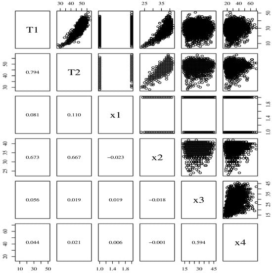
Figure 1.
Scatter plots with their correlations for the indicated variables.
Table 1 provides descriptive statistics for the weight () and length () variables, such as the minimum, median, mean, maximum, standard deviation (SD), coefficient of variation, coefficient of skewness (CS), and coefficient of (excess) kurtosis (CK). For weight, the mean and median are, respectively, and , i.e., the mean is almost equal to the median, which indicates symmetry in the data. The CV is , which means a low level of dispersion around the mean. Furthermore, the CS value suggests slight negative skewness, while the CK indicates a high degree of kurtosis. For length, the mean of and a median of 49, also suggest symmetry in the distribution of data. Moreover, the CV is , showing a low level of dispersion around the mean. The CS indicates a skewed nature and the CK value indicates the high kurtosis feature in the data; see Figure 2 for the plots of histograms for these data. In general, the results support the use of bivariate log-symmetric models as they have flexibility in terms of distributional assumptions and flexibility in describing the behavior of light- and heavy-tailed data.

Table 1.
Summary of the statistics for the newborn dataset.
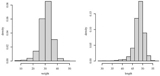
Figure 2.
Histograms for the newborn dataset.
3. Preliminaries
We say that a continuous random vector , with support , follows a bivariate log-symmetric (BLS) distribution with parameters, as follows:
- (medians);
- (dispersion); and
- (correlation)
- for , and density generator [15], denoted by , if its probability density function (PDF) is given by the following:whereand is a partition function given by the following:The variance–covariance matrix, when it exists, of a random vector is given by for some matrix function , where denotes the set of all real matrices, and
Table 2 lists some examples of bivariate log-symmetric distributions, such as the log-normal, log-Student-t, log-hyperbolic, log-Laplace, log-slash, log-power-exponential, and log-logistic. In Table 2, , where , denotes the complete gamma function, , , denotes the Bessel function of the third kind [16], and denotes the lower incomplete gamma function.
Table 2.
Partition functions , density generators , and extra parameters for some BLS distributions.
4. Bivariate Log-Symmetric Regression Models
In this section, we shall introduce the bivariate log-symmetric regression model and discuss parameter estimation based on the maximum likelihood method. Moreover, we also consider residual analysis for the proposed model. The proposed bivariate log-symmetric regression model can be viewed as a generalization of the log-normal/independent linear regression model (in the bivariate case) studied by [14]. Its advantage over the log-normal/independent counterpart lies in its flexibility in describing heteroscedasticity and variable dispersion, as covariates are employed to describe its dispersion and correlation parameters.
4.1. Bivariate Regression
Let , for , be a set of n independent bivariate log-symmetric random variables. We propose a regression model based on the bivariate log-symmetric distribution as follows:
where , , , , and are the vectors of unknown parameters to be estimated, whereas , , , , and are vectors that contain the values of k, l, p, q, and l covariates, respectively. The link functions , , , and in (4)–(8) must be strictly monotone, positive, and at least twice differentiable, with , , , and being the inverse functions of , , , and , respectively. The most common choice for the first four functions is the log link (it does not require to impose non-negativity restrictions on the parameters), whereas for the latter, the most common choice is the ArcTanh link (it guarantees that lies in the interval [−1, 1]). Other common choices for the first four functions are the identity and inverse links, which are often used in generalized linear models. The choice of the appropriate link can be made by using information criteria. A simulation study can be carried out to assess the choice of the link functions. However, it is beyond the scope of this paper and we will address this topic in future work.
4.2. Maximum Likelihood Estimation
Let be a bivariate (not identically distributed) random sample of size n from the BLS distribution (1), with , , and let denote its respective observed value. The log-likelihood function (without the additive constant) for is given by the following:
where
and the vector parameters and , , are connected through equations in (4)–(8). As is differentiable in , the necessary conditions for the occurrence of a maximum (or a possible minimum) are as follows:
known as the likelihood equations. It is a routine task to check the following:
where and
In the above, note that (for ), we have the following:
and
Any nontrivial root of the likelihood equations in (9) is called a maximum likelihood estimator in the loose sense. When the parameter value gives the absolute maximum of the log-likelihood function, it is called a maximum likelihood estimator in the strict sense.
No closed-form solution to the maximization problem is available for the BLS regression model, and a maximum likelihood estimator can only be found via numerical optimization. The extra parameters, associated with the bivariate log-Student-t, log-hyperbolic, log-slash, and log-power-exponential regression models, were estimated by using the profile log-likelihood; see [2]. Under some regularity conditions, Ref. [17] formalized the existence and uniqueness of the maximum likelihood estimator for .
Under some restrictions, Ref. [18] verified that the asymptotic behavior of the maximum likelihood estimator is Gaussian, in other words:
where “” denotes convergence in law, is the zero mean vector, and is the inverse expected Fisher information matrix. It is preferable to use the observed Fisher information, denoted by , instead of [19], because the diagonal elements of the inverse observed Fisher information matrix, denoted by , can be used to approximate the standard errors of the maximum likelihood estimates. The elements of matrix can be found in Appendix A.
4.3. Residual Analysis
Consider a bivariate (not identically distributed) random sample of size n from the BLS distribution (1), with , where , , , , and are defined in (4)–(8), for . By deriving the distribution of the following stochastic relation (see the argument of the function in (1)), we have the following:
where
we propose a residual to assess the goodness of fit and departures from the assumed model. Note that from (13), we have the following:
for , and the corresponding cumulative distribution function (CDF) and PDF of (14) are given, respectively, by the following:
where and are as in (1). We can then use the relation (14) to check the goodness of fit. This is done by contrasting the empirical distribution with the theoretical one through quantile-quantile (QQ) plots.
5. Monte Carlo Simulation
In this section, we present the results of a Monte Carlo simulation study for the BLS regression model. The purpose of this simulation study is to evaluate the performance of the maximum likelihood estimators. For illustrative purposes, we only present the results for the bivariate log-normal model, with simulated data generated according to the following:
for , where , , and are covariates obtained from a standard normal distribution. We consider three different sets of true parameter values, leading to scenarios that cover low, moderate, and high correlations, as follows:
- Scenario 1: , , , and –low correlation–.
- Scenario 2: , , , and –moderate correlation–.
- Scenario 3: , , , and –high correlation–.
- The sample sizes for all three simulation scenarios are , with 500 Monte Carlo replications for each combination of above given parameters.
Table 3 and Table 4 present the results of the Monte Carlo simulation study to assess the performance of the maximum likelihood estimators. In particular, we report the empirical biases and root mean squared errors (RMSEs), which are computed as follows:
where and are the true parameter value and its i-th maximum likelihood estimate, and N is the number of Monte Carlo replications. In terms of parameter recovery, from Table 3 and Table 4, we observe that both biases and RMSEs approach zero as the sample size (n) increases, as expected. We also observe that the bias (RMSE) tends to be larger (smaller) for smaller correlation values.
Table 3.
Empirical biases from simulated bivariate log-normal regression data.
Table 4.
Empirical RMSEs from simulated bivariate log-normal regression data.
6. Application to Newborn Data
We illustrate the proposed methodology with a dataset related to the analysis of anthropometric data of newborns for the diagnosis and prognosis of neonatal health presented in [14] and described in Section 2. We consider the regression structure defined in (4)–(8) for analyzing the newborn data using the bivariate log-symmetric regression model, expressed as follows:
recalling that , with being the weight (in hectograms), , with being the length (crown-heel length, in centimeters), is the sex (0 for female, 1 for male), is the gestational age at birth (in weeks), is the mother’s age (in years) and is the father’s age (in years).
The choice of an appropriate member of the log-symmetric family can be conducted by using information criteria. Table 5 provides the values of the log-likelihood, as well as the Akaike (AIC) and Bayesian information (BIC) criteria for the adjusted bivariate log-symmetric regression models. In general, the bivariate regression model based on the log-slash distribution provides the best fit for the data. The estimated extra parameter for the log-slash model was . For comparison, the values of the log-likelihood, AIC, and BIC for the bivariate gamma regression model [20], a well-accepted bivariate regression approach, are −34,397.03, 68,826.07, and 68,935.06, respectively. Therefore, all the bivariate log-symmetric regression models outperform the gamma one.
Table 5.
Model selection and goodness-of-fit measures for the newborn data.
Figure 3a–g present the QQ plots of the proposed residuals (see Section 4.3) for the models considered in Table 5. By comparing the quantiles of a dataset to the quantiles of a theoretical distribution, the QQ plot can be used to determine whether the dataset follows the reference distribution. From the QQ plots, we observe that the bivariate log-slash model provides the best fit. Therefore, the results of these plots corroborate the ones obtained in Table 5.
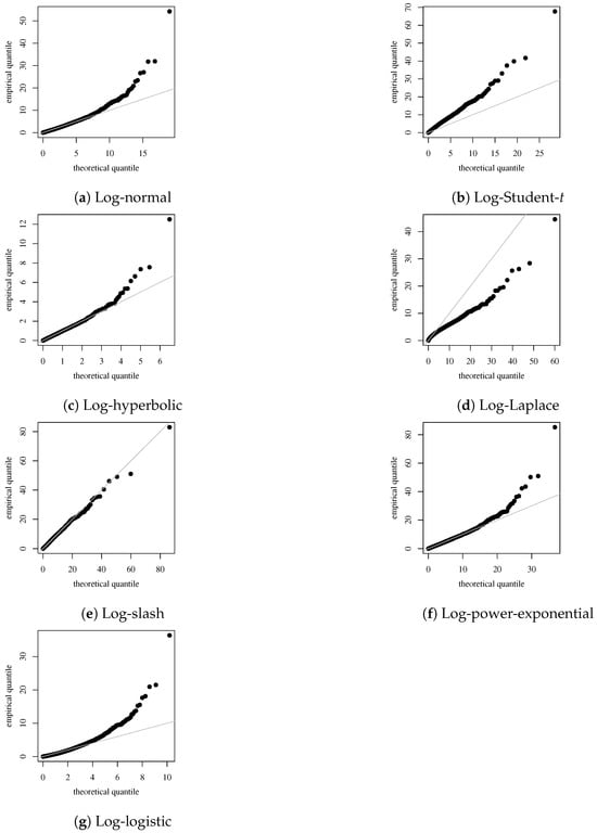
Figure 3.
QQ plot of the residuals for the log-normal, log-Student-t, log-hyperbolic, log-Laplace, log-slash, log-power-exponential, and log-logistic models, respectively.
Table 6 reports the maximum likelihood estimates with SEs, t-values, and p-values for the bivariate log-slash regression model. From this table, we observe the following results: the covariates , , and are significant for and . The covariates and , which impact the dispersion , are significant, and the covariates , , and , which are associated with the dispersion , are significant. Therefore, there is evidence of heteroscedasticity. For the covariates related to the correlation parameter, we observe that , , and are significant.
Table 6.
Maximum likelihood estimates with SEs, t-values, and p-values for the bivariate log-slash regression model for the newborn data.
7. Concluding Remarks
In this paper, we propose a class of regression models based on bivariate log-symmetric distributions. These models offer greater flexibility compared to the bivariate lognormal distribution. In the proposed bivariate regression models, covariates are used to describe the dispersion and correlation parameters, which is an important aspect given the possible presence of heteroscedasticity. We discussed the maximum likelihood estimation of the model parameters and introduced a type of residual. We conducted a Monte Carlo simulation study and demonstrated its application in analyzing anthropometric measurements of newborns. The application to newborn data favored the use of the bivariate log-slash model over other bivariate log-symmetric regression models. Notably, we detected the presence of heteroscedasticity and variable dispersion, features not considered by [14].
Despite the strengths of this study, limitations must be acknowledged. The proposed models have limitations with respect to the presence of nonlinearity. Therefore, addressing non-linear structures that incorporate both parametric and nonparametric components remains an open problem. Moreover, it will be of interest to study bivariate tobit models; see [21]. In addition, influence diagnostic tools can be applied to the proposed models. Furthermore, the behaviors of the Wald, score, likelihood ratio, and gradient tests could also be investigated; see [22]. Finally, comparisons with other approaches such as copula regression can be performed [23]. Work on these issues is currently in progress, and we hope to report the findings in a future paper.
Author Contributions
Conceptualization, H.S., R.V., and R.S.; methodology, H.S., R.V., and R.S.; software, H.S., R.V., and R.S.; validation, H.S., R.V., and R.S.; formal analysis, H.S., R.V., and R.S.; investigation, H.S., R.V., and R.S.; resources, H.S., R.V., and R.S.; data curation, H.S., R.V., and R.S.; writing—original draft preparation, H.S., R.V., and R.S.; writing—review and editing, H.S., R.V., and R.S.; visualization, H.S., R.V., and R.S.; supervision, H.S., R.V., and R.S.; project administration, H.S., R.V., and R.S.; funding acquisition, H.S., R.V., and R.S. All authors have read and agreed to the published version of the manuscript.
Funding
Helton Saulo gratefully acknowledges financial support from: (i) FAP-DF (Fundação de Apoio à Pesquisa do Distrito Federal), Brazil; (ii) the University of Brasilia, Brazil; and (iii) CNPq (Conselho Nacional de Desenvolvimento Científico e Tecnológico), Brazil, through grant numbers 309674/2020-4 and 304716/2023-5.
Informed Consent Statement
Not applicable.
Data Availability Statement
Data are available upon request.
Conflicts of Interest
The authors declare no conflicts of interest.
Appendix A. Elements of Observed Fisher Information Matrix
The observed Fisher information matrix, denoted by , is defined as the negative of the corresponding Hessian matrix. A laborious standard calculation shows that the elements of the Hessian matrix are given by the following:
where , is as in (10), are as in (11) and are as given in (12). Furthermore, in the above, note that (for ), we have the following:
and
References
- Jones, M.C. On reciprocal symmetry. J. Stat. Plan. Inference 2008, 138, 3039–3043. [Google Scholar] [CrossRef]
- Vila, R.; Balakrishnan, N.; Saulo, H.; Protazio, A. Bivariate log-symmetric models: Distributional properties, parameter estimation and an application to public spending data. Braz. J. Probab. Stat. 2023, 37, 619–642. [Google Scholar] [CrossRef]
- Vanegas, L.H.; Paula, G.A. Log-symmetric distributions: Statistical properties and parameter es timation. Braz. J. Probab. Stat. 2016, 30, 196–220. [Google Scholar] [CrossRef]
- Marchant, C.; Leiva, V.; Cysneiros, F. A Multivariate Log-Linear Model for Birnbaum-Saunders Distributions. IEEE Trans. Reliab. 2016, 65, 816–827. [Google Scholar] [CrossRef]
- Kaombe, T.; Banda, J.; Hamuza, G.; Muula, A. Bivariate logistic regression model diagnostics applied to analysis of outlier cancer patients with comorbid diabetes and hypertension in Malawi. Sci. Rep. 2023, 13, 8340. [Google Scholar] [CrossRef]
- Khan, M.; Olivier, J. Regression to the mean: Estimation and adjustment under the bivariate normal distribution. Commun. Stat.-Theory Methods 2023, 52, 6972–6990. [Google Scholar] [CrossRef]
- Umair, M.; Khan, M.; Olivier, J. Accounting for regression to the mean under the bivariate t-distribution. Stat. Methods Med. Res. 2024. [Google Scholar] [CrossRef]
- Saulo, H.; Leão, J.; Leiva, V.; Vila, R.; Tiomazella, V. A bivariate fatigue-life regression model and its application to fracture of metallic tools. Braz. J. Probab. Stat. 2021, 35, 119–137. [Google Scholar] [CrossRef]
- Saulo, H.; Leão, J.; Vila, R.; Leiva, V.; Tiomazella, V. On mean-based bivariate Birnbaum-Saunders distributions: Properties, inference and application. Commun. Stat.-Theory Methods 2020, 49, 6032–6056. [Google Scholar] [CrossRef]
- Paulsen, C.; Nielsen, B.; Msemo, O.; Møller, S.; Ekmann, J.; Theander, T.; Bygbjerg, I.; Lusingu, J.; Minja, T.; Schmiegelow, C. Anthropometric measurements can identify small for gestational age newborns: A cohort study in rural Tanzania. BMC Pediatr. 2019, 19, 120. [Google Scholar] [CrossRef] [PubMed]
- Fenton, T.R.; Kim, J.H. A systematic review and meta-analysis to revisethe Fenton growth chart for preterm infants. BMC Pediatr. 2013, 13, 59. [Google Scholar] [CrossRef] [PubMed]
- Haksari, E.; Lafeber, H.; Hakimi, M.; Pawirohartono, E.; Nyström, L. Reference curves of birth weight, length, and head circumference for gestational ages in Yogyakarta, Indonesia. BMC Pediatr. 2016, 16, 188. [Google Scholar] [CrossRef] [PubMed]
- Rashidi, A.A.; Kiani, O.; Heidarzadeh, M.; Imani, B.; Nematy, M.; Taghipour, A.; Sadr, M.; Norouzy, A. Reference Curves of Birth Weight, Length, and Head Circumference for Gestational Age in Iranian Singleton Births. Iran. J. Pediatr. 2018, 28, e66291. [Google Scholar] [CrossRef]
- Morán-Vásquez, R.; Mazo-Lopera, M.; Ferrari, S. Quantile modeling through multivariate log-normal/independent linear regression models with application to newborn data. Biom. J. 2021, 63, 1290–1308. [Google Scholar] [CrossRef] [PubMed]
- Fang, K.T.; Kotz, S.; Ng, K.W. Symmetric Multivariate and Related Distributions; Chapman and Hall: London, UK, 1990. [Google Scholar]
- Kotz, S.; Kozubowski, T.J.; Podgórski, K. The Laplace Distribution and Generalizations; Wiley: New York, NY, USA, 2001. [Google Scholar]
- Mäkeläinen, T.; Schmidt, K.; Styan, G. On the existence and uniqueness of the maximum likelihood estimate of a vector-valued parameter in fixed-size samples. Ann. Stat. 1981, 9, 758–767. [Google Scholar] [CrossRef]
- Cramér, H. Mathematical Methods of Statistics; Princeton University Press: Princeton, NJ, USA, 1946. [Google Scholar]
- Efron, B.; Hinkley, D. Assessing the accuracy of the maximum likelihood estimator: Observed versus expected Fisher Information. Biometrika 1978, 65, 457–487. [Google Scholar] [CrossRef]
- Hu, S.; Murphy, T.B.; O’Hagan, A. Bivariate Gamma Mixture of Experts Models for Joint Insurance Claims Modeling. arXiv 2019. [Google Scholar] [CrossRef]
- Yoo, S.H. Analysing household bottled water and water purifier expenditures: Simultaneous equation bivariate Tobit model. Appl. Econ. Lett. 2005, 12, 297–301. [Google Scholar] [CrossRef]
- Saulo, H.; Dasilva, A.; Leiva, V.; Sánchez, L.; de la Fuente-Mella, H. Log-symmetric quantile regression models. Stat. Neerl. 2022, 76, 124–163. [Google Scholar] [CrossRef]
- Song, P.X.K.; Li, M.; Yuan, Y. Joint Regression Analysis of Correlated Data Using Gaussian Copulas. Biometrics 2009, 65, 60–68. [Google Scholar] [CrossRef] [PubMed]


Disclaimer/Publisher’s Note: The statements, opinions and data contained in all publications are solely those of the individual author(s) and contributor(s) and not of MDPI and/or the editor(s). MDPI and/or the editor(s) disclaim responsibility for any injury to people or property resulting from any ideas, methods, instructions or products referred to in the content. |
© 2024 by the authors. Licensee MDPI, Basel, Switzerland. This article is an open access article distributed under the terms and conditions of the Creative Commons Attribution (CC BY) license (https://creativecommons.org/licenses/by/4.0/).