Modeling and Simulation of an Integrated Synchronous Generator Connected to an Infinite Bus through a Transmission Line in Bond Graph

Abstract

Most electrical energy generation systems are based on synchronous generators; as a result, their analysis always provides interesting findings, especially if an approach different to those traditionally studied is used. Therefore, an approach involving the modeling and simulation of a synchronous generator connected to an infinite bus through a transmission line in a bond graph is proposed. The behavior of the synchronous generator is analyzed in four case studies of the transmission line: (1) a symmetrical transmission line, where the resistance and inductance of the three phases $(a,b,c)$ are equal, which determine resistances and inductances in coordinates $(d,q,0)$ as individual decoupled elements; (2) a symmetrical transmission line for the resistances and for non-symmetrical inductances in coordinates $(a,b,c)$ that result in resistances that are individual decoupled elements and in a field of inductances in coordinates $(d,q,0)$; (3) a non-symmetrical transmission line for resistances and for symmetrical inductances in coordinates $(a,b,c)$ that produce a field of resistances and inductances as individual elements decoupled in coordinates $(d,q,0)$; and (4) a non-symmetrical transmission line for resistances and inductances in coordinates $(a,b,c)$ that determine resistances and inductance fields in coordinates $(d,q,0)$. A junction structure based on a bond graph model that allows for obtaining the mathematical model of this electrical system is proposed. Due to the characteristics of a bond graph, model reduction can be carried out directly and easily. Therefore, reduced bond graph models for the four transmission line case studies are proposed, where the transmission line is seen as if it were inside the synchronous generator. In order to demonstrate that the models obtained are correct, simulation results using the 20-Sim software are shown. The simulation results determine that for a symmetrical transmission line, currents in the generator in the d and q axes are −25.87 A and 0.1168 A, while in the case of a non-symmetrical transmission line, these currents are −26.14 A and 0.0211 A, showing that for these current magnitudes, the generator is little affected due to the parameters of the generator and the line. However, for a high degree of non-symmetry of the resistances in phases a, b and c, it causes the generator to reach an unstable condition, which is shown in the last simulation of the paper.

1. Introduction

Most electric power generation systems contain synchronous generators connected to transmission lines to deliver power to consumers. These generators determine nonlinear systems due to the interaction between electrical, magnetic and mechanical variables. The models used for synchronous generators in systems interconnected with transmission lines and supply to loads are frequently reduced. However, reduced models of synchronous generators may not describe in detail the behavior of their variables. On the other hand, reduced models are justified due to the complexity of the systems.

The first stage in the analysis of electrical power systems is the development of models of the energy supply sources, that is, the synchronous generators. Some of the main references in the modeling and simulation of electrical machines and especially synchronous machines are found in [1,2,3]. The transient modeling of the synchronous machine in the Simulink software is developed in [4]. The stability characteristics through eigenvalues of the synchronous machine are proposed in [5]. The analysis of power transmission lines where the simulation is improved by adding capacitance in parallel to the series inductance is described in [6] and the modeling of three-phase power transformers and their simulation is explained in [7].

Different approaches and analyses of synchronous generators in interconnected systems schemes are described in the following references. The electromechanical oscillations of a synchronous generator due to load voltages are found in [8]. Electromechanical transients in power systems with transmission and distribution lines are presented in [9]. The application of virtual synchronous generators to interpret characteristics external to synchronous generators is introduced in [10]. The small-signal analysis of multi-machines in large-scale power systems is studied in [11]. The behavior of the excitation angle and the control of a synchronous generator in a small-signal scheme are described in [12].

Some important references of links of electrical systems in different approaches are cited below. The properties of transients in three-phase networks with unbalanced sources are investigated in [13]. The study of the availability of transfer capacity in ultra-high voltage networks in China is analyzed in [14]. The simulation of transmission lines using the Dynamic Harmonic Domain (DHD) is found in [15]. The characteristics of failures at measurement points of long-distance and huge-capacity transmission lines and their adaptation to common transmission lines are simulated in [16]. The mathematical modeling of a power network formed by ordinary differential equations and transmission lines with distributed parameters represented by partial differential equations is proposed in [17]. The challenge of configuring microgrids for power supply and charging that can lead to effective energy management systems is discussed in [18]. A management architecture model using a supervisory control and data acquisition approach in a building with laboratory measurements is proposed in [19]. A small-signal stability analysis for multi-machine systems connected to a microgrid is presented in [20].

Currently, it is essential to refer to advances in electrical power systems with renewable sources as follows: a small-signal stability analysis of a power system formed by a synchronous generator, photovoltaic panels and their connection to an infinite bus is established in [21]. The possibility of electromechanical oscillations between synchronous machines and renewable generation converters is investigated in [22]. A power system formed by generators and transmission networks, where the variation in the inertia constant of the generator causes oscillations in the rotor, is discussed in [23]. A control strategy in the energy supply with renewable sources for small-signal stability analysis is proposed in [24]. A small-signal grid model with control schemes for synchronous capacitor-and-inverter-based sources is developed in [25]. The effect of irradiance and temperature of a photovoltaic panel connected to a three-phase network is studied in [26]. Doubly fed induction generators connected to power converters that control wind turbines in a power system are proposed in [27]. Different reference frames of a three-phase system connected to the grid and current regulators are analyzed in [28].

Bond graph is a graphical modeling theory that has been used to represent systems formed by various energy domains (electrical, mechanical, hydraulic, magnetic, thermal) in a unified way. A large number of references have been published on the modeling of various systems [29,30]. Subsequently, structural properties of systems such as stability, controllability, observability and decoupling in bond graphs have been published [31,32,33].

Some of the advantages of bond graph modeling over other methods are as follows:

• A bond graph can determine models of linear, nonlinear, time-varying systems with concentrated or distributed parameters in a clear and simple way.
• A bond graph allows for knowing the linearly independent or dependent state variables from the causality of the storage elements, while in other modeling methods they are not clear.
• The properties of structural controllability and structural observability are obtained from causal trajectories without requiring the mathematical model of the system.
• The steady state response of the state variables for a linear system or for a class of nonlinear systems requires calculating the inverse matrix of states; in a bond graph, this inverse matrix is obtained by changing the causality of the storage elements.
• If there is a change in the system configuration in a bond graph, it only requires including those changes, and in traditional methods, it is generally necessary to obtain the model from the beginning. This feature is very interesting for the analysis of system failures.
• Model reduction in a bond graph is obtained by knowing the causal relationships between the elements, while in traditional methods, it can be carried out with an in-dept knowledge of the model.
• A bond graph allows for obtaining models formed by systems with various energy domains (electrical, mechanical, hydraulic, thermal, magnetic) such as the synchronous generator, which is an electromechanical system, and the relationships of the electrical and mechanical variables can be directly known.

Some disadvantages of bond graphs are as follows:

• Although the scientific community knows bond graph modeling, the properties have not been fully disseminated and its application sometimes requires an in-depth knowledge of bond graph.
• Some systems may have problems in the application of causality and this may lead to introducing auxiliary elements to the system that are only known by bond graph experts.
• Systems with switching elements such as power electronics require careful consideration in the choice of switching elements.
• Due to the unified characteristics that the bond graph uses (momentum, displacement, effort and flow), obtaining other variables is not direct and care is required.

The process of obtaining the structural controllability and structural observability of systems modeled in a bond graph is presented in [34]. The design of state observers in the bond graph approach is proposed in [30]. The determination of Lagrangian and Hamiltonian models from the representation of systems in a bond graph is established in [35].

Recently, some advances and applications in bond graphs have been published and are described below. Modeling and simulation including control strategies applied to gearboxes in transmission systems are found in [36]. The application of the virtual power principle for systems with mechanical constraints in bond graphs is developed in [37]. The modeling of a power MOSFET and a PiN diode in a bond graph for a Buck converter system is proposed in [38]. The performance prediction applied to line-start permanent-magnet synchronous motors considering electrical, magnetic and mechanical energy domains in bond graphs is developed in [39]. The bond graph modeling of a hybrid photovoltaic fuel-cell electrolyzer battery system including energy interactions between hydraulic, thermal, electromechanical, thermodynamic and electrical fields is presented in [40]. The application of a bond graph to the design of a Boost converter in an attempt to improve the efficiency of and reduction in losses is found in [41]. The modeling of the blades of a wind turbine in a bond graph to determine the dynamic behavior is proposed in [42]. The acquisition mechanism applied to a power generation system with wave energy using a bond graph is proposed in [43].

Some works published on bond graphs that have modeled and used synchronous generators are as follows: the mathematical and bond graph development of a basic synchronous generator is proposed in [44]. A model of the synchronous generator in a bond graph to perform a phasor analysis is presented in [45]. The modeling of a synchronous generator integrated into a skystream wind turbine is proposed in [46]. The direct linearization of the synchronous generator with multibond graphs is proposed in [47]. Likewise, the modeling of three-phase electrical systems with a multibond graph without considering synchronous or other types of generators is introduced in [48]. These references indicate that there is still no developed work on the synchronous generator within an electrical power system in a bond graph; therefore, with the proposed paper, progress can be made in this area.

Some recent references that may contribute to the state of the art of the proposed paper are as follows: A comparative analysis of the behavior of single-fed and double-fed induction generators in which a wind turbine is applied and modeled in a bond graph is proposed in [49]. Bond graph modeling for the diagnosis of a double-fed induction generator is proposed in [50]; this diagnosis us used for fault detection and isolation. Bond graph modeling of a hybrid power system formed by wind energy and solar energy is presented in [51]. the installation of a pumping system consisting of a photovoltaic generator, a wind turbine, converters and induction motors based on bond graph models is proposed in [52].

An optimal fault-tolerant control applied to multiphase permanent-magnet synchronous machines to mitigate vibrations and noise is introduced in [53]. A comparative analysis of two control strategies applied to power converters to reduce power system oscillations is analyzed in [54]. The removal of a DC-offset to avoid effects on the synchronization of three-phase systems is carried out in an SRF-PLL unit, which is proposed in [55]. The generalized magnetic-equivalent circuit modeling technique applied to synchronous reluctance motors is presented in [56]. A permanent-magnet synchronous generator with bolting and an overhang structure to reduce scattering problems is analyzed in [57]. The transition of a power system from the inadequate concept of classical synchronization stability to the new form of synchronization with non-synchronous generators, along with three technical challenges, are proposed in [58].

Thus, electrical machines and especially synchronous generators have been modeled in bond graphs showing the energy exchange of the electrical and mechanical subsystems. However, the analysis of synchronous generators in electrical power system diagrams in bond graphs has not been analyzed in relation to the references of traditional power systems obtained in the abovementioned studies.

Therefore, in this paper, the modeling of an electrical power system formed by a synchronous generator connected to an infinite bus through a transmission line is proposed. Bond graph modeling is carried out in coordinates $\left(d,q,0\right)$, indicating the generator and the transmission line. Unbalanced models of the transmission line are presented and their effect on the synchronous generator is analyzed. Because a bond graph is very useful in model reduction, reduced models of the different cases of balanced and unbalanced transmission lines connected to the synchronous generator are proposed. These reduced bond graphs show a system where the transmission line is introduced to the synchronous generator. Therefore, the behavior of the synchronous generator variables with the implications of the transmission line are obtained directly. Four case studies of transmission lines connected to the synchronous generator are modeled. Likewise, a bond graph junction structure related to the mathematical description of electric power systems is proposed. In order to show how the influence of the transmission line on the generator variables is, simulation results are obtained.

The main contribution of this paper is to analyze the behavior of the synchronous generator by considering the transmission line in a bond graph, and that reduced models can be obtained in a bond graph that clearly indicates that the transmission line is introduced internally to the generator. The novelty of this proposal is that the behavior of the generator can be known directly without requiring analysis in stages since the transmission line has been included in the generator.

Section 2 summarizes the synchronous generator connection to an infinite bus through a transmission line in the traditional scheme. Section 3 proposes a junction structure based on a bond graph model to obtain the mathematical model in state space for electrical systems. In addition, bond graphs for different cases of transmission lines are proposed and reduced models in the physical domain are introduced. The behavior of the generator variables are obtained through simulations in Section 4. Finally, the conclusions are given in Section 5.

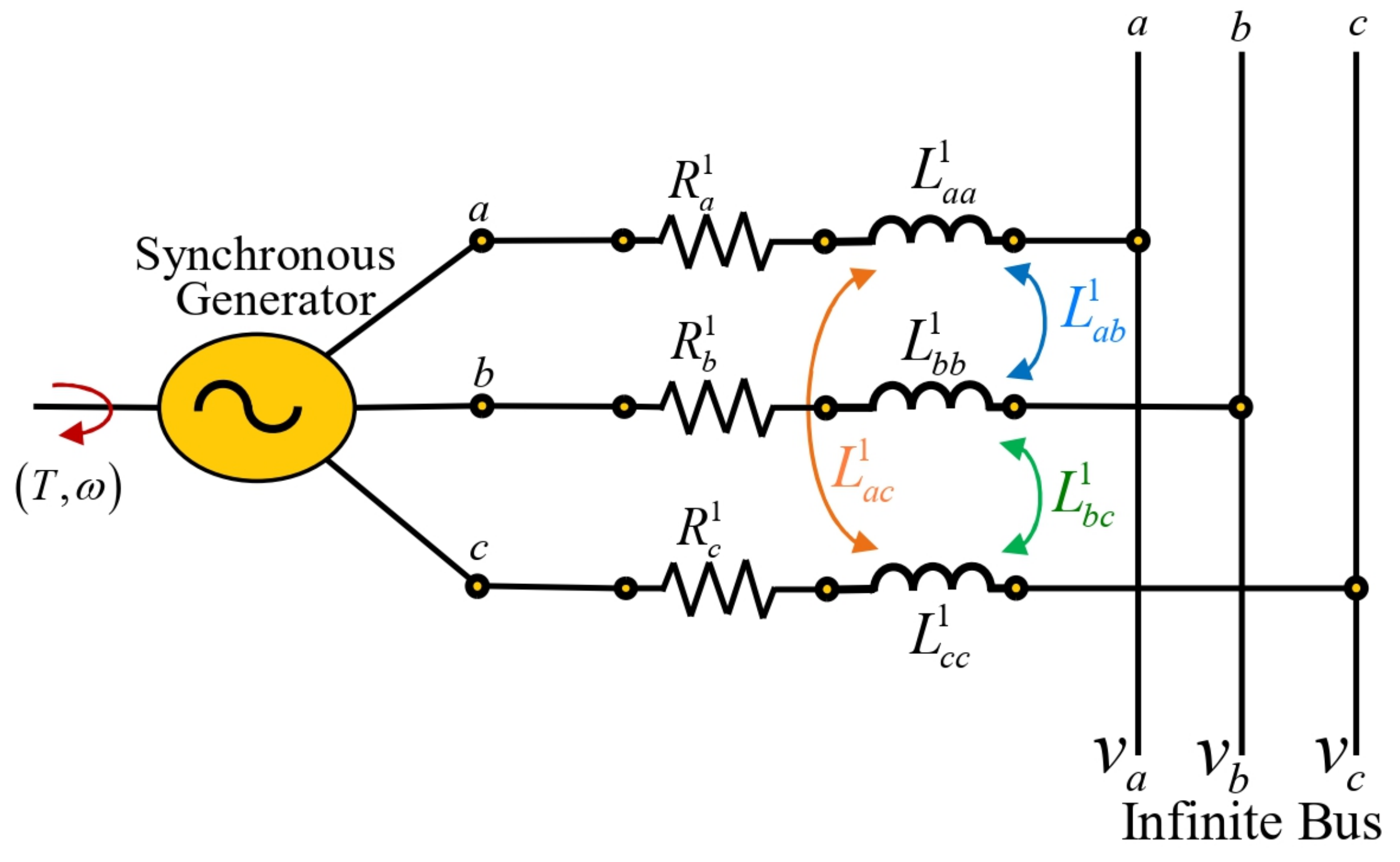
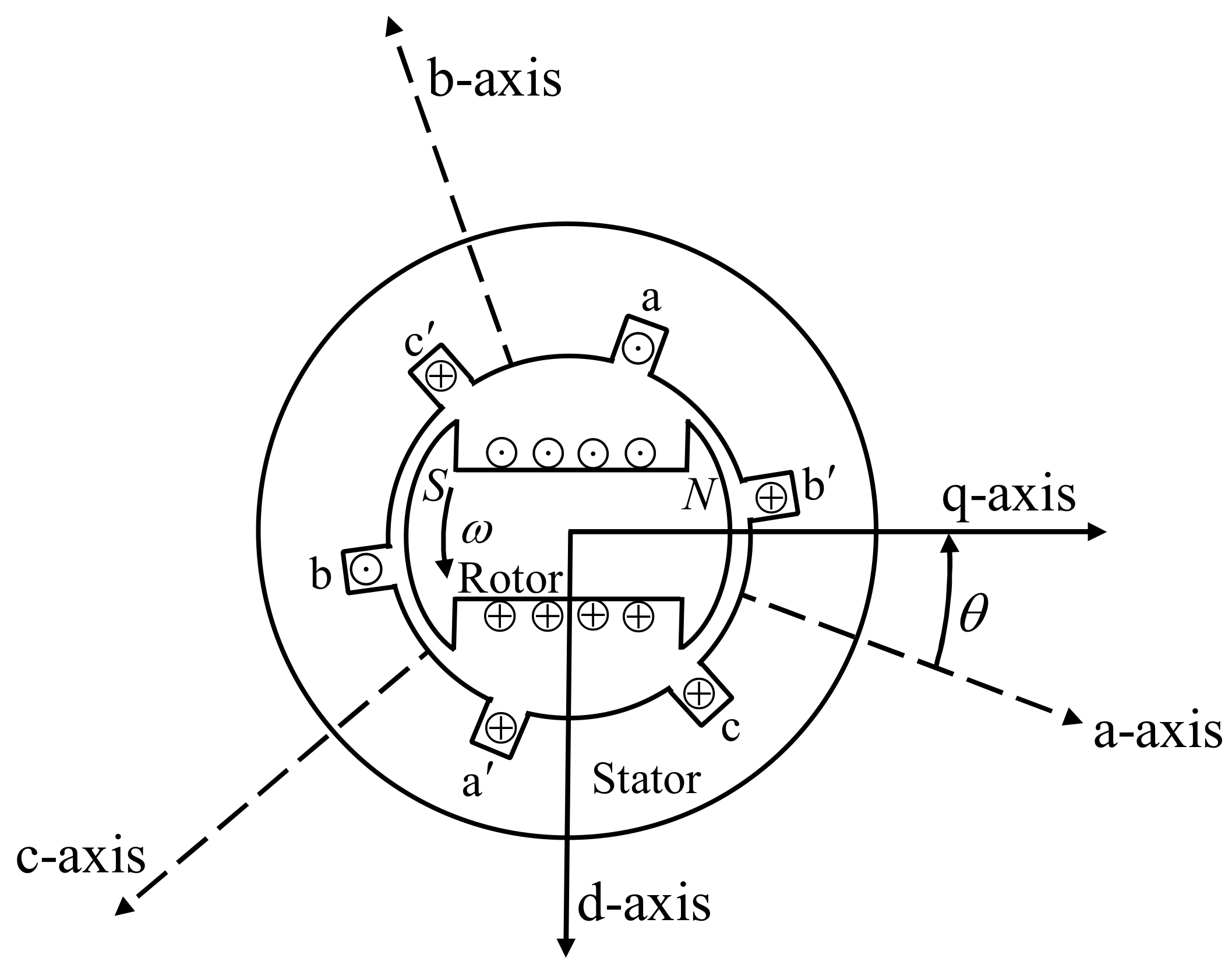
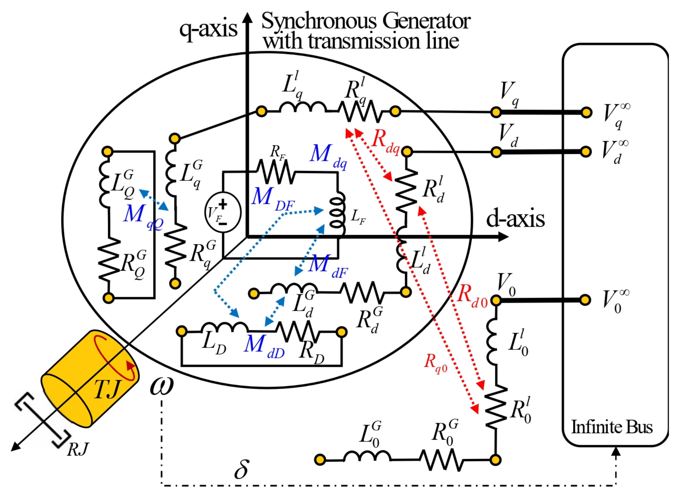
2. Classical Modeling of a Synchronous Generator—Infinite Bus

A synchronous generator (SG) connected to an infinite bus through a transmission line is shown in Figure 1 [1,2,3].

The voltage balance in coordinates $\left(a,b,c\right)$ in this generation system is defined by

$$v_{abc}^G=v_{abc}^{\infty }+R_{abc}^l{i}_{abc}+L_{abc}^l{\displaystyle \frac{d{i}_{abc}}{dt}}$$

(1)

where the voltages at the terminals of the SG $v_{abc}^G$ are given by

$$v_{abc}^G=\left[\begin{array}{c}{v}_a^G\\ v_b^G\\ v_c^G\end{array}\right]$$

(2)

The currents supplied by the SG to the infinite bus are

$$i_{abc}=\left[\begin{array}{c}{i}_a\\ i_b\\ i_c\end{array}\right]$$

(3)

The voltages on the infinite bus are

$$v_{abc}^{\infty }=\left[\begin{array}{c}{v}_a^{\infty }\\ v_b^{\infty }\\ v_c^{\infty }\end{array}\right]$$

(4)

The resistances in the transmission line are described as

$$R_{abc}^l=\left[\begin{array}{ccc}{R}_a^l& 0& 0\\ 0& R_b^l& 0\\ 0& 0& R_c^l\end{array}\right]$$

(5)

For a balanced three-phase system, $R_a^l=R_b^l=R_c^l$, and the magnetic couplings of the transmission line are expressed as

$$L_{abc}^l=\left[\begin{array}{ccc}{L}_{aa}^l& L_{ab}^l& L_{ac}^l\\ L_{ab}^l& L_{bb}^l& L_{bc}^l\\ L_{ac}^l& L_{bc}^l& L_{cc}^l\end{array}\right]$$

(6)

The expression given in (1) determines a time-varying nonlinear system that makes analysis and a possible controller design difficult. Therefore, in three-phase electrical systems, the application of the Park transformation allows for a reduction in the complexity of the problem.

The Park transformation is a mathematical tool that is applied to electrical machines that allows for the time dependence to be eliminated from the equations. The Park transformation changes the variables and parameters of the phases $\left(a,b,c\right)$ to a reference frame that moves with the machine rotor. This reference frame is designated by the coordinates $\left(d,q,0\right)$ and is defined by [1,2,3]

$$v_{dq0}=P{v}_{abc}$$

(7)

where

$$P=\sqrt{{\displaystyle \frac{2}{3}}}\left[\begin{array}{ccc}cos\theta & cos\left(\theta -{\displaystyle \frac{2\pi }{3}}\right)& cos\left(\theta +{\displaystyle \frac{2\pi }{3}}\right)\\ sin\theta & sin\left(\theta -{\displaystyle \frac{2\pi }{3}}\right)& sin\left(\theta +{\displaystyle \frac{2\pi }{3}}\right)\\ {\displaystyle \frac{1}{\sqrt{2}}}& {\displaystyle \frac{1}{\sqrt{2}}}& {\displaystyle \frac{1}{\sqrt{2}}}\end{array}\right]$$

(8)

with

$$\theta =wt+\delta +{\displaystyle \frac{\pi }{2}}$$

(9)

where w is the angular frequency in $rad/s$, and $\delta$ is the synchronous torque angle. For currents and flow links,

$$\begin{array}{ccc}\hfill i_{dq0}& =& \hfill P{i}_{abc}\hfill \end{array}$$

(10)

$$\begin{array}{ccc}\hfill {\lambda }_{dq0}& =& \hfill P{\lambda }_{abc}\hfill \end{array}$$

(11)

Applying the Park transformation to (1) yields the following expression:

$$v_{dq0}^G=P{v}_{abc}^G=P{v}_{abc}^{\infty }+P{R}_{abc}^l{P}^{-1}P{i}_{abc}+P{L}_{abc}^l{P}^{-1}P{\displaystyle \frac{d{i}_{abc}}{dt}}$$

(12)

$$v_{dq0}^G=v_{dq0}^{¨\infty }+R_{dq0}^l{i}_{dq0}+L_{dq0}^l\left[{\displaystyle \frac{d{i}_{dq0}}{dt}}-{\displaystyle \frac{dP}{dt}}{P}^{-1}{i}_{dq0}\right]$$

(13)

where

$$\begin{array}{ccc}\hfill v_{dq0}^G& =& \hfill P{v}_{abc}^G\hfill \end{array}$$

(14)

$$\begin{array}{ccc}\hfill v_{dq0}^{¨\infty }& =& \hfill P{v}_{abc}^{\infty }\hfill \end{array}$$

(15)

$$\begin{array}{ccc}\hfill R_{dq0}^l& =& \hfill P{R}_{abc}^l{P}^{-1}\hfill \end{array}$$

(16)

$$\begin{array}{ccc}\hfill L_{dq0}^l& =& \hfill P{L}_{abc}^l{P}^{-1}\hfill \end{array}$$

(17)

Re-writing

$$v_{dq0}^G=v_{dq0}^{¨\infty }+R_{dq0}^l{i}_{dq0}+L_{dq0}^l{\displaystyle \frac{d{i}_{dq0}}{dt}}-L_{dq0}^{l}X\left(w\right)i_{dq0}$$

(18)

where

$$X\left(w\right)=\left[\begin{array}{ccc}0& -w& 0\\ w& 0& 0\\ 0& 0& 0\end{array}\right]$$

(19)

and for a balanced supply voltage,

$$v_{dq0}^{¨\infty }=\sqrt{3}{V}_m\left[\begin{array}{c}-sin\delta \\ cos\delta \\ 0\end{array}\right]$$

(20)

with $V_m$ as the maximum bus voltage in coordinates $\left(a,b,c\right)$.

A schematic diagram of an SG is shown in Figure 2. This machine is built with three windings in the stator $\left(a,b,c\right)$ and one winding in the rotor $\left(F\right)$. The conditions of the SG are as follows:

• In the air gap path, the stator windings have a sinusoidal distribution.
• The rotor inductances with respect to the position of the machine axis do not vary due to the stator slots.
• Magnetic saturation effects are not taken into account.
• The effects of magnetic hysteresis are negligible.

A representation of the SG with its equivalent circuits in coordinates $\left(a,b,c\right)$ is illustrated in Figure 3. Each stator winding is formed by its resistance and inductance $\left(R_a,L_a\right),$$\left(R_b,L_b\right)$ and $\left(R_c,L_c\right)$. The field winding located on the rotor has its resistance and inductance $\left(R_F,L_F\right)$ with the supply DC voltage $\left(V_F\right)$. Additionally, two damping windings to account for electromechanical transients are included. The mechanical subsystem is modeled with the inertia of the machine $\left(T_J\right)$ and the friction with the air $\left(R_J\right)$. The power generated is obtained by the currents $\left(i_a,i_b,i_c\right)$ and voltages $\left(v_a,v_b,v_c\right)$ in the phases.

The mathematical model of this SG of Figure 3 in coordinates $\left(d,q,0\right)$ has been established in [1,2,3] and is given by

$$\left[\begin{array}{cccccc}{L}_d^G& M_{dD}& M_{dF}& 0& 0& 0\\ M_{dD}& L_D& M_{DF}& 0& 0& 0\\ M_{dF}& M_{DF}& L_F& 0& 0& 0\\ 0& 0& 0& L_q^G& M_{qQ}& 0\\ 0& 0& 0& M_{qQ}& L_Q& 0\\ 0& 0& 0& 0& 0& T_J\end{array}\right]{\displaystyle \frac{d}{dt}}\left[\begin{array}{c}{i}_d\\ i_D\\ i_F\\ i_q\\ i_Q\\ w\end{array}\right]=\left[\begin{array}{cccccc}-R_d^G& 0& 0& 0& 0& -{\lambda }_q\\ 0& -R_D& 0& 0& 0& 0\\ 0& 0& -R_F& 0& 0& 0\\ 0& 0& 0& -R_q^G& 0& {\lambda }_d\\ 0& 0& 0& 0& -R_Q& 0\\ {\lambda }_q& 0& 0& -{\lambda }_d& 0& -R_J\end{array}\right]\left[\begin{array}{c}{i}_d\\ i_D\\ i_F\\ i_q\\ i_Q\\ w\end{array}\right]+\left[\begin{array}{c}{v}_d^G\\ 0\\ v_F\\ v_q^G\\ 0\\ T_m\end{array}\right]$$

(21)

where the currents and voltages in the armature winding in coordinates $\left(d,q,0\right)$ are $\left(i_d,i_q\right)$ and $\left(v_d,v_q\right)$, respectively; the currents in the damping winding are $\left(i_D,i_Q\right)$; $\left(i_F,v_F\right)$ denote the current and voltage in the field winding, respectively; and w is the velocity of the machine rotor. The self-inductances and resistances of the armature winding in coordinates $\left(d,q,0\right)$ are $\left(L_d^G,L_q^G\right)$ and $\left(R_d^G,R_q^G\right)$, respectively. The self-inductances and resistances of the damping winding are $\left(L_D,L_Q\right)$ and $\left(R_D,R_Q\right)$, respectively; $\left(L_F,R_F\right)$ denote the self-inductance and resistance of the field winding; the mutual inductances in the d and q axes are $\left(M_{dD},M_{dF},M_{DF}\right)$ and $\left(M_{qQ}\right)$, respectively; $\left(T_J,R_J\right)$ represent the inertia and friction with the air of the rotor shaft of the machine; $\left(T_m\right)$ is the input torque to the SG and $\left({\lambda }_d,{\lambda }_q\right)$ denote the flux linkage in the d and q axes, respectively.

The connection of an SG to an infinite bus with different cases of transmission line parameters in a bond graph approach is proposed in the next section.

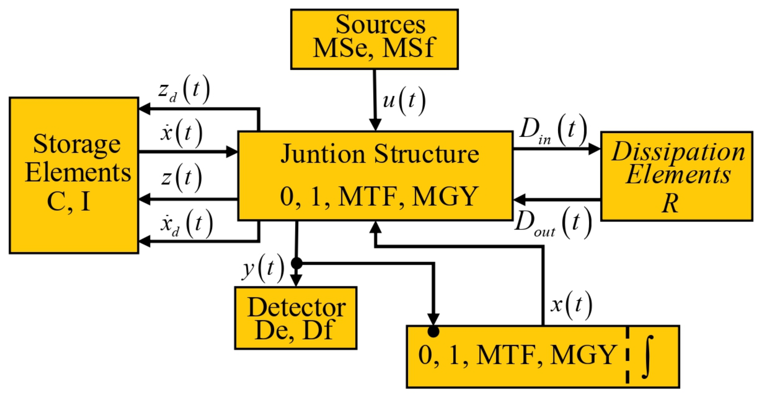
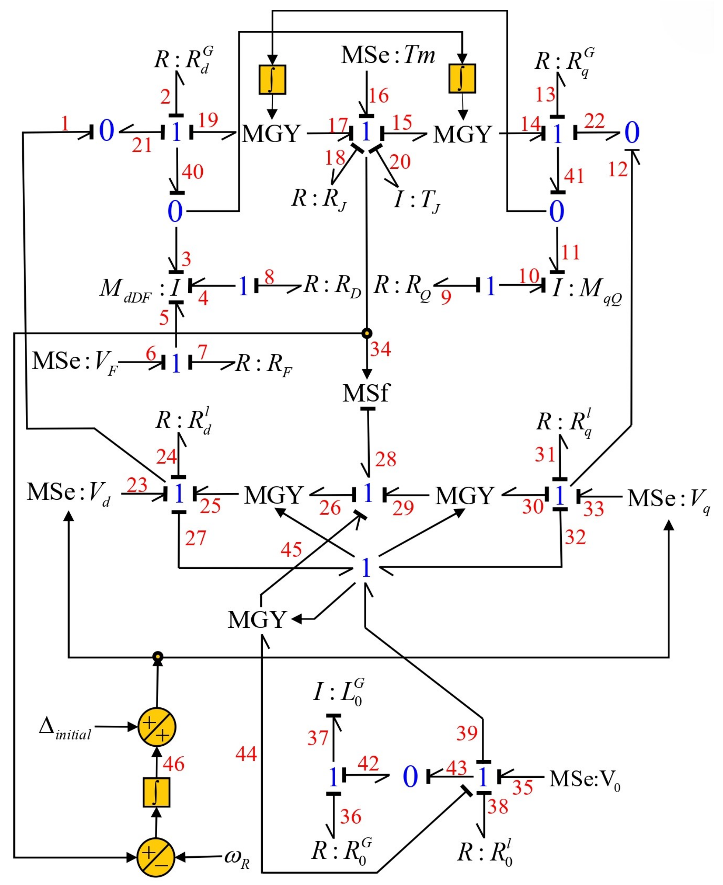
3. Synchronous Generator—Infinite Bus in a Bond Graph Approach

The bond graph (BG) is a very useful methodology in modeling systems formed with different energy domains. However, various mathematical models can be obtained from a bond graph model; likewise, the analysis and control of these bond graph systems or their mathematical models can be carried out.

Hence, the different blocks that are part of a BG that represent an SG connected to an infinite bus are shown in Figure 4.

The description of the blocks whose elements from the BG of Figure 4 determine the following fields and key vectors:

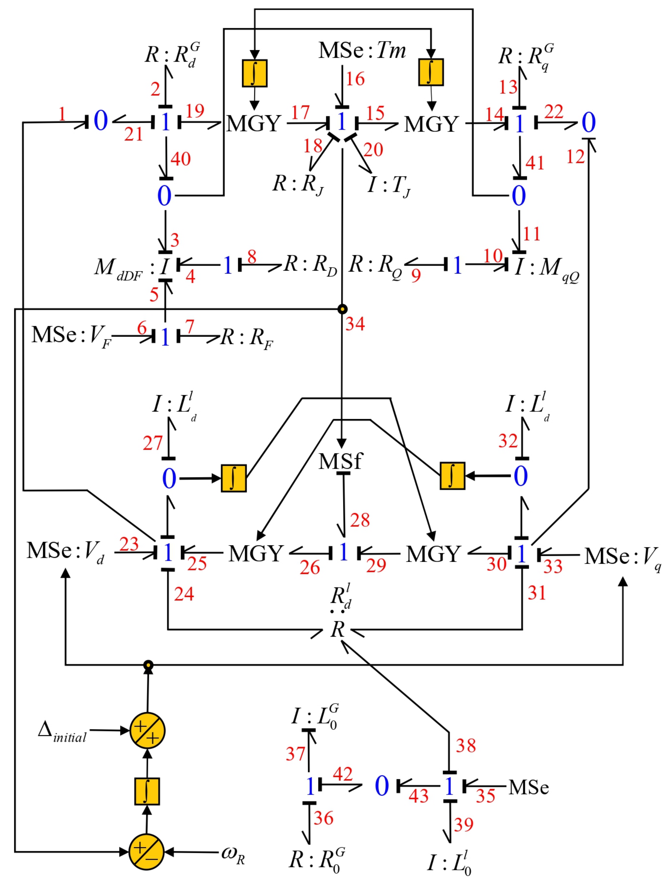
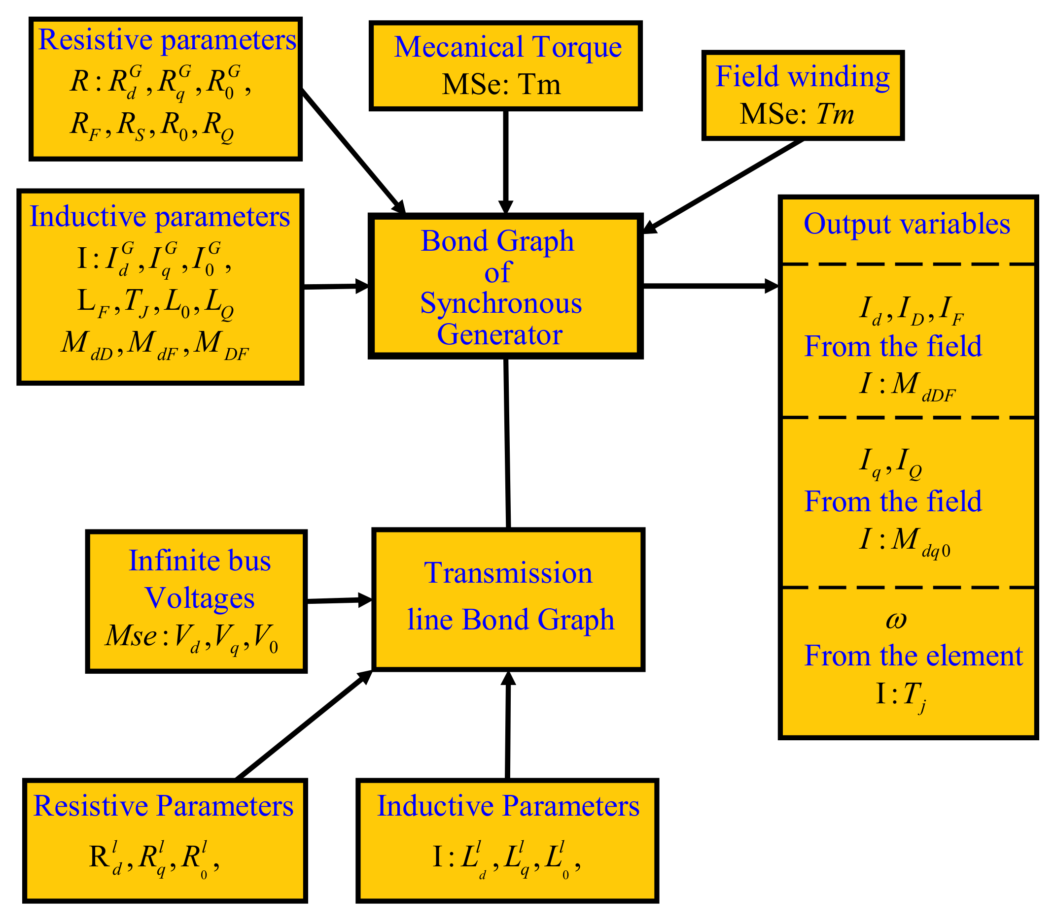
• Power supply is through the source field $\left(M{S}_e,M{S}_f\right)$ with input vector $u\left(t\right)$$\in {\Re }^p$.
• The linearly independent state variables $x\left(t\right)$$\in {\Re }^n$ are obtained from the storage elements $\left(C,I\right)$ in integral causality assignment that determine the energy and co-energy defined by $z\left(t\right)$$\in {\Re }^n$.
• The linearly dependent state variables $x_d\left(t\right)$$\in {\Re }^m$ that determine energy are obtained from the storage elements $\left(C,I\right)$ in derivative causality assignment, and the co-energy of these elements is given by $z\left(t\right)$$\in {\Re }^m$.
• The energy dissipation elements $\left(R\right)$ are expressed by $D_{in}\left(t\right)$$\in {\Re }^r$ and $D_{out}\left(t\right)$$\in {\Re }^r$.
• The system outputs $y\left(t\right)$$\in {\Re }^q$ are obtained from the detection field $\left(D{S}_e,D{S}_f\right)$.
• The main junction structure $\left(0,1,MTF,MGY\right)$ that determines the interconnection of the different fields of the bond graph is formed by the junctions $\left(0,1\right)$ and by the modulated transformers and gyrators $\left(MTF,MGY\right).$
• The junction substructure $\left(0,1,TF,GY,\int \right)$ is required to be the variables that modulate $\left(MTF,MGY\right)$.

The mathematical model of the system shown in Figure 4 is proposed from the following Lemma 1.

Lemma 1.

Consider a BG whose storage elements have a predefined integral causality assignment and contains transformers or/and gyrators modulated by state variables that represent a class of nonlinear systems where the junction structure is defined by

$$\left[\begin{array}{c}\stackrel{•}{x}\left(t\right)\\ D_{in}\left(t\right)\\ y\left(t\right)\\ z_d\left(t\right)\end{array}\right]=\left[\begin{array}{cccc}{S}_{11}\left(x\right)& S_{12}\left(x\right)& S_{13}\left(x\right)& S_{14}\left(x\right)\\ S_{21}\left(x\right)& S_{22}\left(x\right)& S_{23}\left(x\right)& 0\\ S_{31}\left(x\right)& S_{32}\left(x\right)& S_{33}\left(x\right)& 0\\ S_{41}\left(x\right)& 0& 0& 0\end{array}\right]\left[\begin{array}{c}z\left(t\right)\\ D_{out}\left(t\right)\\ u\left(t\right)\\ {\stackrel{•}{x}}_d\left(t\right)\end{array}\right]$$

(22)

with constitutive relations

$$\begin{array}{ccc}\hfill D_{out}x\left(t\right)& =& \hfill L{D}_{in}\left(t\right)\hfill \end{array}$$

(23)

$$\begin{array}{ccc}\hfill z\left(t\right)& =& \hfill Fx\left(t\right)\hfill \end{array}$$

(24)

$$\begin{array}{ccc}\hfill z_d\left(t\right)& =& \hfill F_d{x}_d\left(t\right)\hfill \end{array}$$

(25)

Therefore, a mathematical model in state space according to electrical power systems is described as

$$E\left(x\right)\stackrel{•}{z}\left(t\right)=A\left(x\right)z\left(t\right)+B\left(x\right)u\left(t\right)$$

(26)

where

$$\begin{array}{ccc}\hfill E\left(x\right)& =& \hfill F^{-1}-S_{14}\left(x\right)F_d^{-1}{S}_{41}\left(x\right)\hfill \end{array}$$

(27)

$$\begin{array}{ccc}\hfill A\left(x\right)& =& \hfill S_{11}\left(x\right)+S_{12}\left(x\right)M\left(x\right)S_{21}\left(x\right)+S_{14}\left(x\right)F_d^{-1}{\stackrel{•}{S}}_{41}\left(x\right)\hfill \end{array}$$

(28)

$$\begin{array}{ccc}\hfill B\left(x\right)& =& \hfill S_{13}\left(x\right)+S_{12}\left(x\right)M\left(x\right)S_{23}\left(x\right)\hfill \end{array}$$

(29)

with

$$M\left(x\right)=L{\left[I-S_{22}\left(x\right)L\right]}^{-1}$$

(30)

Proof. 

Starting from the second line of (22) with (23),

$$D_{in}\left(t\right)={\left[I-S_{22}\left(x\right)L\right]}^{-1}\left[S_{21}\left(x\right)z\left(t\right)+S_{23}\left(x\right)u\left(t\right)\right]$$

(31)

and the fourth line of (22) with (24) and (25), the relationships of the storage elements in derivative causality are described as

$${\stackrel{•}{x}}_d\left(t\right)=F_d^{-1}{S}_{41}\left(x\right)F\stackrel{•}{x}\left(t\right)+F_d^{-1}{\stackrel{•}{S}}_{41}\left(x\right)Fx\left(t\right)$$

(32)

Substituting (31) and (32),

$$\begin{array}{ccc}\hfill \stackrel{•}{x}\left(t\right)& =& \hfill S_{11}\left(x\right)z\left(t\right)+S_{12}\left(x\right)L{\left[I-S_{22}\left(x\right)L\right]}^{-1}\left[S_{21}\left(x\right)z\left(t\right)+S_{23}\left(x\right)u\left(t\right)\right]+\hfill \\ & & \hfill S_{13}\left(x\right)u\left(t\right)+S_{14}\left(x\right)\left[F_d^{-1}{S}_{41}\left(x\right)F\stackrel{•}{x}\left(t\right)+F_d^{-1}{\stackrel{•}{S}}_{41}\left(x\right)Fx\left(t\right)\right]\hfill \end{array}$$

(33)

It is common to describe the mathematical model in state space for electrical power systems in terms of co-energy $\left(z:e\leftrightarrow v,f\leftrightarrow i\right)$ and not in terms of energy state variables $\left(z:e\leftrightarrow v,f\leftrightarrow i\right)$; this way,

$$\stackrel{•}{x}\left(t\right)=F^{-1}\stackrel{•}{z}\left(t\right)$$

(34)

and substituting (33) in (34),

$$\begin{array}{ccc}\hfill \left[I-S_{14}\left(x\right)F_d^{-1}{S}_{41}\left(x\right)F\right]F^{-1}\stackrel{•}{z}\left(t\right)& =& \hfill \left[S_{11}\left(x\right)+S_{12}\left(x\right)M\left(x\right)S_{21}\left(x\right)+S_{14}\left(x\right)F_d^{-1}{\stackrel{•}{S}}_{41}\left(x\right)\right]z\left(t\right)+\hfill \\ & & \hfill \left[S_{13}\left(x\right)+S_{12}\left(x\right)M\left(x\right)S_{23}\left(x\right)\right]u\left(t\right)\hfill \end{array}$$

(35)

where $M\left(x\right)=L{\left[I-S_{22}\left(x\right)L\right]}^{-1};$ from (27)–(29) and (35), Equation (26) is proven. □

Below, depending on the characteristics of the transmission line, four cases are presented.

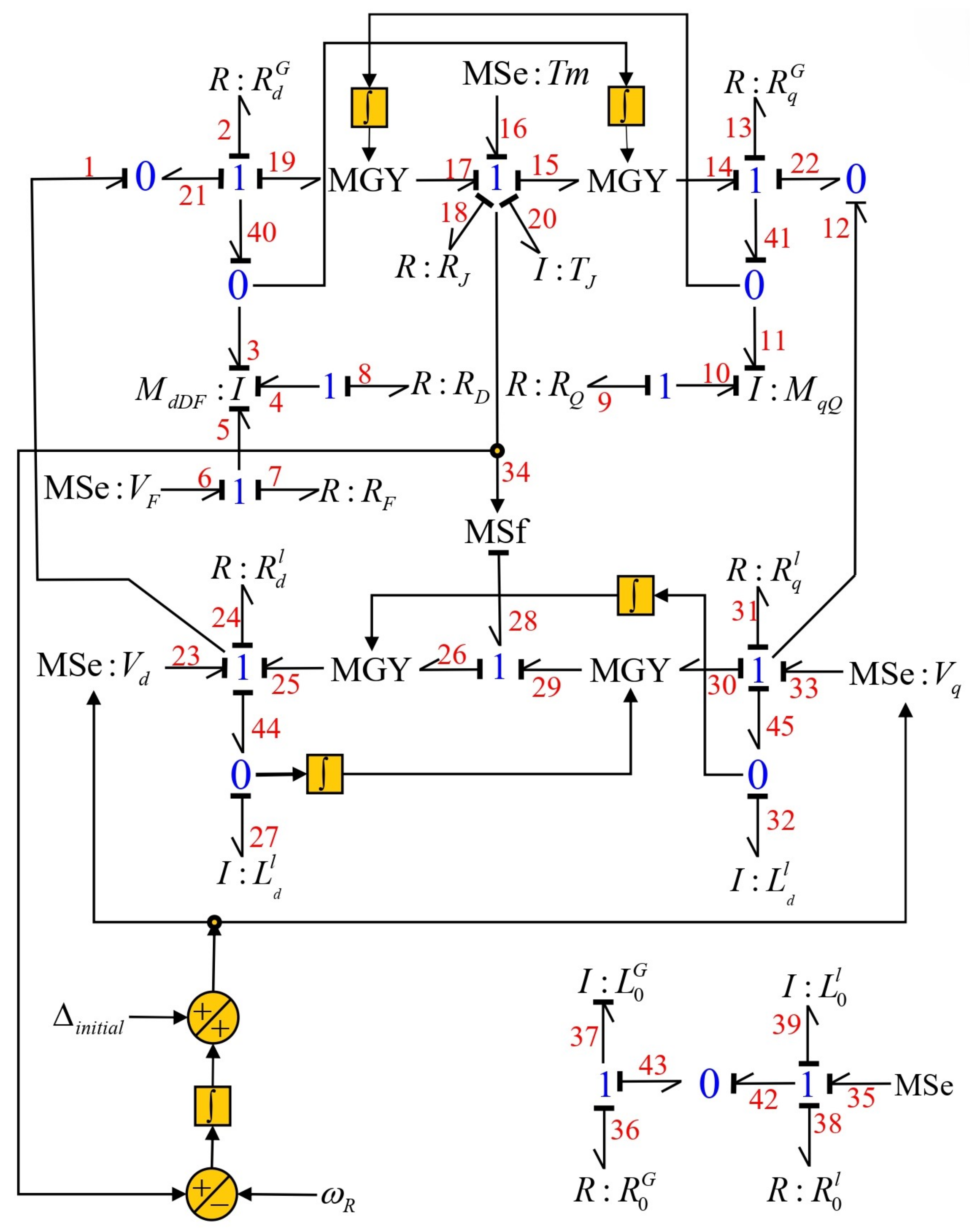
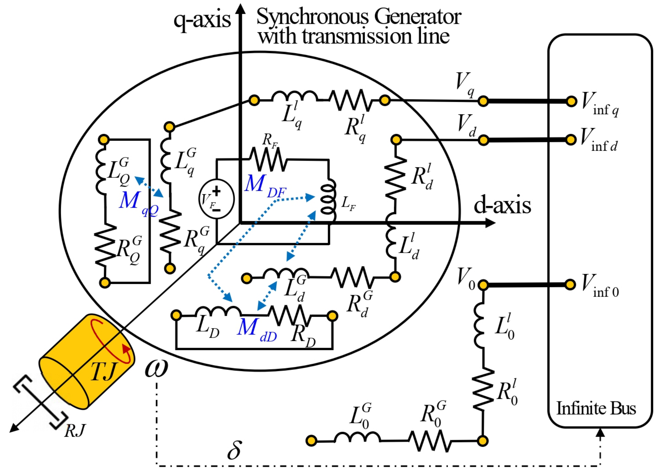
3.1. Case 1: Symmetrical Transmission Line

The most common and simplest case of a transmission line is that it represents a balanced system, so the impedance matrix of the three-phase line in coordinates $\left(a,b,c\right)$ is given by

$$\begin{array}{ccc}\hfill R_{abc}^l& =& \hfill \left[\begin{array}{ccc}{R}_l& 0& 0\\ 0& R_l& 0\\ 0& 0& R_l\end{array}\right]\hfill \end{array}$$

(36)

$$\begin{array}{ccc}\hfill L_{abc}^l& =& \hfill \left[\begin{array}{ccc}{L}_l& 0& 0\\ 0& L_l& 0\\ 0& 0& L_l\end{array}\right]\hfill \end{array}$$

(37)

In this case, the resistance and inductance of the transmission line are the same in all three phases and there are no mutual effects between the phases. Applying the Park transformation to (36) and (37) gives the following:

$$\begin{array}{ccc}\hfill R_{dq0}^l& =& \hfill \left[\begin{array}{ccc}{R}_d^l& 0& 0\\ 0& R_q^l& 0\\ 0& 0& R_0^l\end{array}\right]\hfill \end{array}$$

(38)

$$\begin{array}{ccc}\hfill L_{dq0}^l& =& \hfill \left[\begin{array}{ccc}{L}_d^l& 0& 0\\ 0& L_q^l& 0\\ 0& 0& L_0^l\end{array}\right]\hfill \end{array}$$

(39)

where $R_d^l=R_q^l=R_0^l$ and $L_d^l=L_q^l=L_0^l$.

The BG corresponding to the SG connected to this transmission line with the infinite bus in coordinates $\left(d,q,0\right)$ is shown in Figure 5.

The elements that form the BG in Figure 5 are as follows:

• $R:R_d^G$, $R:R_q^G$ and $R:R_0^G$ denote the resistances in coordinates $\left(d,q,0\right)$, respectively.
• $R:R_D$ and $R:R_Q$ are the two damper windings on the d and q axes, respectively.
• The rotor circuit, called the field winding, is formed by the resistance and inductances $R:R_F$ and $I:L_F$, respectively, and the supply voltage to this winding $M{S}_e:V_F$.
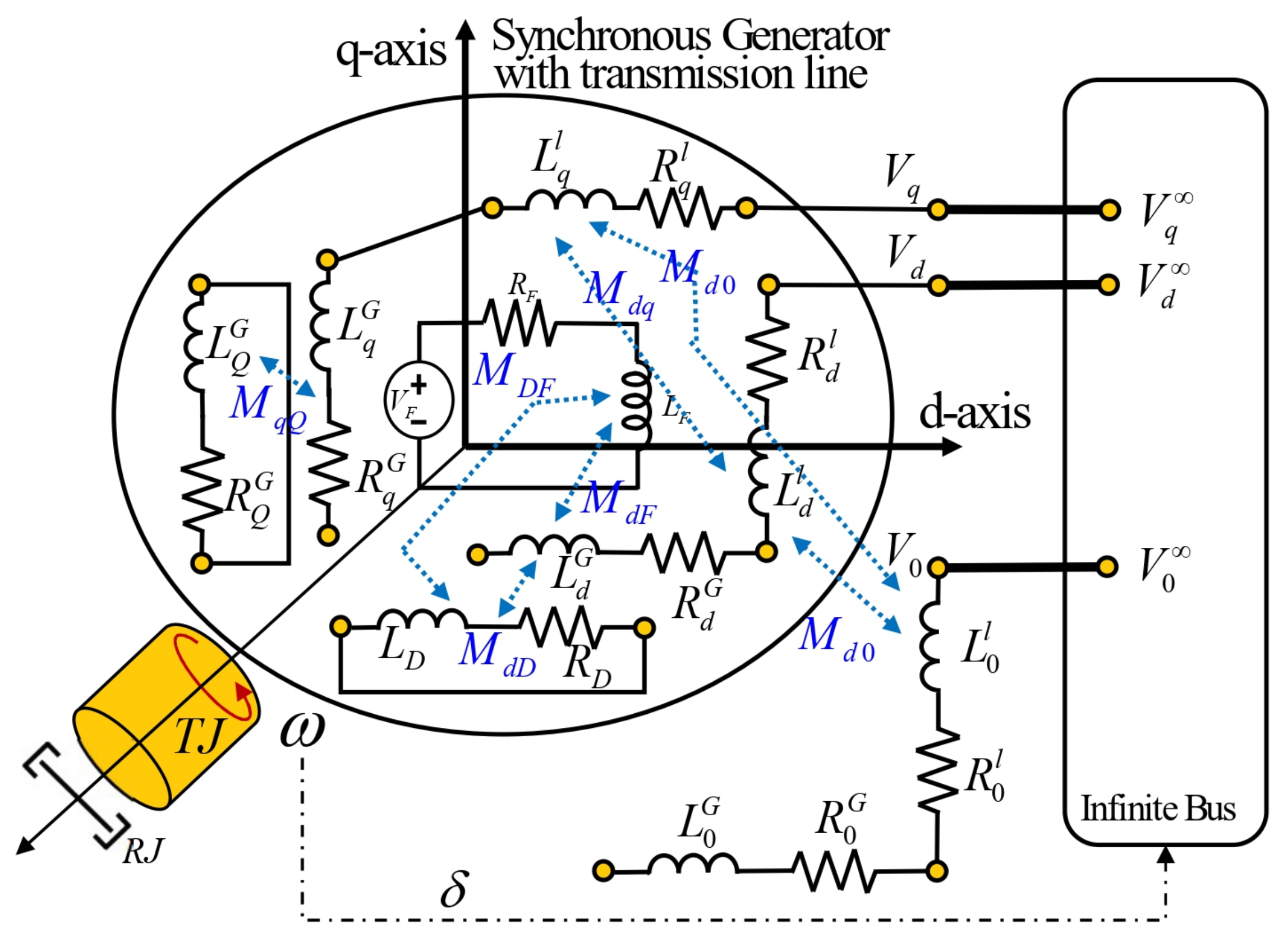
• The field of the storage elements for the generator on the d axis $I:M_{dqF}$ is defined by the constitutive relation given in (42) and contains the self-inductances $L_d^G$, $L_D$ and $L_F$ and the mutual inductances $M_{dD}$, $M_{dF}$ and $M_{DF}$.
• The field of the storage elements for the generator on the q axis $I:M_{qQ}$ is defined by the constitutive relation given in (43) and contains the self-inductances $L_q^G$ and $L_Q$ and the mutual inductance $M_{qQ}$.
• In the mechanical subsystem, $I:T_J$ is denoted as the inertia of the generator, $R:R_J$ as the friction with the air and $M{S}_e:T_m$ is the input torque to the generator.
• The elements of the transmission line are $\left(R:R_d^l,R:R_q^l,R:R_0^l\right)$ and $\left(I:L_d^l,I:L_q^l,I:L_0^l\right)$; they denote the resistances and inductances in the coordinates $\left(d,q,0\right)$, respectively.
• The supply voltages on the infinite bus are $\left(M{S}_e:V_d^{\infty },M{S}_e:V_q^{\infty },M{S}_e:V_0^{\infty }\right)$ in the coordinates $\left(d,q,0\right)$, respectively.

The key vectors of the BG are described as

$$\begin{array}{ccc}\hfill x& =& \hfill \left[\begin{array}{c}{p}_3\\ p_4\\ p_5\\ p_{11}\\ p_{10}\\ p_{37}\\ p_{18}\end{array}\right];\stackrel{•}{x}=\left[\begin{array}{c}{e}_3\\ e_4\\ e_5\\ e_{11}\\ e_{10}\\ e_{37}\\ e_{18}\end{array}\right];z=\left[\begin{array}{c}{f}_3\\ f_4\\ f_5\\ f_{11}\\ f_{10}\\ f_{37}\\ f_{18}\end{array}\right];D_{in}=\left[\begin{array}{c}{f}_2\\ f_8\\ f_7\\ f_{13}\\ f_9\\ f_{20}\\ f_{36}\\ f_{24}\\ f_{31}\\ f_{38}\end{array}\right];D_{out}=\left[\begin{array}{c}{e}_2\\ e_8\\ e_7\\ e_{13}\\ e_9\\ e_{20}\\ e_{36}\\ e_{24}\\ e_{31}\\ e_{38}\end{array}\right]\hfill \\ \hfill x_d& =& \hfill \left[\begin{array}{c}{p}_{27}\\ p_{32}\\ p_{39}\end{array}\right];{\stackrel{•}{x}}_d=\left[\begin{array}{c}{e}_{27}\\ e_{32}\\ e_{39}\end{array}\right];z=\left[\begin{array}{c}{f}_{27}\\ f_{32}\\ f_{39}\end{array}\right];u=\left[\begin{array}{c}{e}_{23}\\ e_{33}\\ e_6\\ e_{35}\\ e_{16}\end{array}\right]\hfill \end{array}$$

(40)

The constitutive relations for the storage elements in an integral causality assignment are given by

$$F^{-1}=diag\left\{M_{dFD},M_{qQ},L_0^G,T_J\right\}$$

(41)

where

$$\begin{array}{ccc}\hfill M_{dFD}& =& \hfill \left[\begin{array}{ccc}{L}_d^G& M_{dD}& M_{dF}\\ M_{dD}& L_D& M_{DF}\\ M_{dF}& M_{DF}& L_F\end{array}\right]\hfill \end{array}$$

(42)

$$\begin{array}{ccc}\hfill M_{qQ}& =& \hfill \left[\begin{array}{cc}{L}_q^G& M_{qQ}\\ M_{qQ}& L_Q\end{array}\right]\hfill \end{array}$$

(43)

for the storage elements in a derivative causality assignment

$$F_d^{-1}=diag\left\{L_d^l,L_q^l,L_0^l\right\}$$

(44)

and for the dissipation elements:

$$L=diag\left\{R_d^G,R_D,R_F,R_q^G,R_Q,R_J,R_0^G,R_d^l,R_q^l,R_0^l\right\}$$

(45)

The junction structure is described as

$$\begin{array}{ccc}\hfill S_{11}& =& \hfill \left[\begin{array}{ccccccc}0& 0& 0& 0& 0& 0& -{\lambda }_q^G-{\lambda }_q^l\\ 0& 0& 0& 0& 0& 0& 0\\ 0& 0& 0& 0& 0& 0& 0\\ 0& 0& 0& 0& 0& 0& {\lambda }_d^G+{\lambda }_d^l\\ 0& 0& 0& 0& 0& 0& 0\\ 0& 0& 0& 0& 0& 0& 0\\ {\lambda }_q^G& 0& 0& {\lambda }_d^G& 0& 0& 0\end{array}\right];S_{12}=\left[\begin{array}{cccccccccc}-1& 0& 0& 0& 0& 0& 0& 1& 0& 0\\ 0& -1& 0& 0& 0& 0& 0& 0& 0& 0\\ 0& 0& -1& 0& 0& 0& 0& 0& 0& 0\\ 0& 0& 0& -1& 0& 0& 0& 0& 1& 0\\ 0& 0& 0& 0& -1& 0& 0& 0& 0& 0\\ 0& 0& 0& 0& 0& -1& 0& 0& 0& 1\\ 0& 0& 0& 0& 0& 0& -1& 0& 0& 0\end{array}\right]\hfill \\ \hfill S_{13}& =& \hfill \left[\begin{array}{ccccc}-1& 0& 0& 0& 0\\ 0& 0& 0& 0& 0\\ 0& 0& 1& 0& 0\\ 0& -1& 0& 0& 0\\ 0& 0& 0& 0& 0\\ 0& 0& 0& 0& -1\\ 0& 0& 0& 1& 0\end{array}\right];S_{14}=\left[\begin{array}{ccc}1& 0& 0\\ 0& 0& 0\\ 0& 0& 0\\ 0& 1& 0\\ 0& 0& 0\\ 0& 0& 1\\ 0& 0& 0\end{array}\right];S_{21}=\left[\begin{array}{ccccccc}1& 0& 0& 0& 0& 0& 0\\ 0& 1& 0& 0& 0& 0& 0\\ 0& 0& 1& 0& 0& 0& 0\\ 0& 0& 0& 1& 0& 0& 0\\ 0& 0& 0& 0& 1& 0& 0\\ 0& 0& 0& 0& 0& 1& 0\\ 0& 0& 0& 0& 0& 0& 1\\ -1& 0& 0& 0& 0& 0& 0\\ 0& 0& 0& -1& 0& 0& 0\\ 0& 0& 0& 0& 0& 0& -1\end{array}\right]\hfill \\ \hfill S_{41}& =& \hfill \left[\begin{array}{ccccccc}-1& 0& 0& 0& 0& 0& 0\\ 0& 0& 0& -1& 0& 0& 0\\ 0& 0& 0& 0& 0& 0& -1\end{array}\right];S_{22}=S_{23}=0\hfill \end{array}$$

(46)

In order to determine the mathematical model of the system, the proposed lemma is applied. From (27) with (41), (44) and (46), the matrix $E\left(x\right)$ is given by

$$E\left(x\right)=\left[\begin{array}{ccccccc}\widehat{L_d}& M_{dD}& M_{dD}& 0& 0& 0& 0\\ M_{dD}& L_D& M_{DF}& 0& 0& 0& 0\\ M_{dD}& M_{DF}& L_F& 0& 0& 0& 0\\ 0& 0& 0& \widehat{L_q}& M_{qQ}& 0& 0\\ 0& 0& 0& M_{qQ}& L_Q& 0& 0\\ 0& 0& 0& 0& 0& \widehat{L_0}& 0\\ 0& 0& 0& 0& 0& 0& T_J\end{array}\right]$$

(47)

where

$$\widehat{L_d}=L_d^G+L_d^l;\widehat{L_q}=L_q^G+L_q^l;\widehat{L_0}=L_0^G+L_0^l$$

(48)

From (28) and (30) with (45) and (46), the state matrix is defined by

$$A\left(x\right)=\left[\begin{array}{ccccccc}-\widehat{R_d}& 0& 0& 0& 0& 0& -{\lambda }_q^G-{\lambda }_q^l\\ 0& -R_D& 0& 0& 0& 0& 0\\ 0& 0& -R_F& 0& 0& 0& 0\\ 0& 0& 0& -\widehat{R_q}& 0& 0& {\lambda }_d^G+{\lambda }_d^l\\ 0& 0& 0& 0& -R_Q& 0& 0\\ 0& 0& 0& 0& 0& -\widehat{R_0}& 0\\ {\lambda }_q^G& 0& 0& -{\lambda }_d^G& 0& 0& -R_J\end{array}\right]$$

(49)

where

$$\widehat{R_d}=R_d^G+R_d^l;\widehat{R_q}=R_q^G+R_q^l;\widehat{R_0}=R_0^G+R_0^l$$

(50)

From (29) and (30) with (45) and (46), the input matrix is defined by

$$B\left(x\right)=\left[\begin{array}{ccccc}-1& 0& 0& 0& 0\\ 0& 0& 0& 0& 0\\ 0& 0& 1& 0& 0\\ 0& -1& 0& 0& 0\\ 0& 0& 0& 0& 0\\ 0& 0& 0& 1& 0\\ 0& 0& 0& 0& 1\end{array}\right]$$

(51)

One of the advantages of modeling systems in BG is the possibility of obtaining reduced bond graphs (RBGs) that are equivalent to the original system. Therefore, in this paper, it is proposed to incorporate the transmission line into the SG model, and a RBG is obtained, which is shown in Figure 6.

It is evident that the RBG is fundamentally the BG of the SG, where the resistances $R_d^G$ and $R_q^G$ are added to the resistances of the transmission line, and the same happens with the self-inductances $L_d^G$ and $L_q^G$. Note that there are no longer elements in derivative causality, which allows there to be no difficulties in the numerical solution.

The key vectors of this RBG for x, $\stackrel{•}{x}$, z and u are those described in (40), but for the dissipation elements, they are

$$D_{in}={\left[\begin{array}{ccccccc}{f}_2& f_8& f_7& f_{13}& f_9& f_{36}& f_{20}\end{array}\right]}^T;D_{out}={\left[\begin{array}{ccccccc}{e}_2& e_8& e_7& e_{13}& e_9& e_{36}& e_{20}\end{array}\right]}^T$$

(52)

and the constitutive relations are

$$F^{-1}=diag\left\{\widehat{M_{dFD}},\widehat{M_{qQ}},L_0^G,T_J\right\}$$

(53)

where

$$\begin{array}{ccc}\hfill \widehat{M_{dFD}}& =& \hfill \left[\begin{array}{ccc}\widehat{L_d}& M_{dD}& M_{dF}\\ M_{dD}& L_D& M_{DF}\\ M_{dF}& M_{DF}& L_F\end{array}\right]\hfill \end{array}$$

(54)

$$\begin{array}{ccc}\hfill \widehat{M_{qQ}}& =& \hfill \left[\begin{array}{cc}\widehat{L_q}& M_{qQ}\\ M_{qQ}& L_Q\end{array}\right]\hfill \end{array}$$

(55)

$$L=diag\left\{\widehat{R_d},R_D,R_F,\widehat{R_q},R_Q,R_J,\widehat{R_0}\right\}$$

(56)

The junction structure of this RBG is given by

$$\begin{array}{ccc}\hfill S_{11}& =& \hfill \left[\begin{array}{cc}0& S_{11}^{12}\\ S_{11}^{21}& 0\end{array}\right];S_{13}=\left[\begin{array}{ccccc}-1& 0& 0& 0& 0\\ 0& 0& 0& 0& 0\\ 0& 0& 1& 0& 0\\ 0& -1& 0& 0& 0\\ 0& 0& 0& 0& 0\\ 0& 0& 0& 0& -1\\ 0& 0& 0& 1& 0\end{array}\right]\hfill \\ \hfill S_{12}& =& \hfill -S_{21}=-I;S_{22}=S_{23}=0\hfill \end{array}$$

(57)

where

$$S_{11}^{21}=-{\left(S_{11}^{12}\right)}^T=\left[\begin{array}{cccccc}\widehat{{\lambda }_q}& 0& 0& -\widehat{{\lambda }_d}& 0& 0\end{array}\right]$$

(58)

with

$$\widehat{{\lambda }_q}=\left[\begin{array}{cc}\widehat{L_q}& M_{qQ}\end{array}\right]\left[\begin{array}{c}{f}_{11}\\ f_{10}\end{array}\right];\widehat{{\lambda }_d}=\left[\begin{array}{ccc}\widehat{L_d}& M_{dD}& M_{dF}\end{array}\right]\left[\begin{array}{c}{f}_3\\ f_4\\ f_5\end{array}\right]$$

(59)

Since this RBG has no elements in derivative causality, then $E\left(x\right)=F^{-1}$, because $S_{12}=-S_{21}=-I$ and the state matrix can be obtained with $S_{11}$ as the elements on the diagonal formed by (56) proving (49), and the input matrix given by (51) is directly the $S_{13}$ of (57). Therefore, it is proven that the RBG represents the mathematical model of this case 1 in the connection of a synchronous generator to a transmission line with the defined characteristics.

A physical meaning of the RBG is shown in Figure 7 where the transmission line is connected in series with the internal elements of the generator and there is no major change in the system.

3.2. Case 2: Variable Inductances

Another interesting case is when the system is not completely balanced; the resistances in the three are equal $R_{abc}^l=\left[\begin{array}{ccc}{R}_l& 0& 0\\ 0& R_l& 0\\ 0& 0& R_l\end{array}\right]$ but the inductance matrix in coordinates $\left(a,b,c\right)$ is defined by

$$L_{abc}^l=\left[\begin{array}{ccc}{L}_a& M_{ab}& M_{ac}\\ M_{ab}& L_b& M_{bc}\\ M_{ac}& M_{bc}& L_c\end{array}\right]$$

(60)

In this case, the inductances of each of the phases are different and the mutual inductances are also different; this case is common in unbalanced systems or with some failure in the phases. Applying the Park transformation to (60) results in

$$L_{dq0}^l=\left[\begin{array}{ccc}{L}_d^l& M_{dq}^l& M_{d0}^l\\ M_{dq}^l& L_q^l& M_{q0}^l\\ M_{d0}^l& M_{q0}^l& L_0^l\end{array}\right]$$

(61)

The BG of this case is shown in Figure 8.

Fortunately, the key vectors of this BG in Figure 8 are the same as the BG in Figure 5. The only difference is the constitutive relationship of the storage elements in derivative causality, so (44) is changed by

$$F_d^{-1}=M_{qd0}^l=\left[\begin{array}{ccc}{L}_d^l& M_{dq}& M_{d0}\\ M_{dq}& L_q^l& M_{q0}\\ M_{d0}& M_{q0}& L_0^l\end{array}\right]$$

(62)

The junction structure is almost the same with respect to (46), except the submatrix $S_{11}$ is defined by

$$S_{11}=\left[\begin{array}{ccccccc}0& 0& 0& 0& 0& 0& -{\lambda }_q^G-{\lambda }_1\\ 0& 0& 0& 0& 0& 0& 0\\ 0& 0& 0& 0& 0& 0& 0\\ 0& 0& 0& 0& 0& 0& {\lambda }_d^G+{\lambda }_2\\ 0& 0& 0& 0& 0& 0& 0\\ 0& 0& 0& 0& 0& 0& {\lambda }_3\\ {\lambda }_q^G& 0& 0& {\lambda }_d^G& 0& 0& 0\end{array}\right]$$

(63)

where

$$\begin{array}{ccc}\hfill {\lambda }_1& =& \hfill L_d^l{i}_q-M_{qQ}^l{i}_d\hfill \end{array}$$

(64)

$$\begin{array}{ccc}\hfill {\lambda }_2& =& \hfill L_q^l{i}_d-M_{dq}^l{i}_q\hfill \end{array}$$

(65)

$$\begin{array}{ccc}\hfill {\lambda }_3& =& \hfill M_{q0}^l{i}_d-M_{d0}^l{i}_q\hfill \end{array}$$

(66)

Since (62) is defined by a field $-I$ of inductances of the transmission line, then from (27), with (41), (62) and (46) of the matrix $E\left(x\right)$,

$$E\left(x\right)=\left[\begin{array}{ccccccc}\widehat{L_d}& M_{dD}& M_{dD}& M_{dq}& 0& M_{d0}& 0\\ M_{dD}& L_D& M_{DF}& 0& 0& 0& 0\\ M_{dD}& M_{DF}& L_F& 0& 0& 0& 0\\ M_{dq}& 0& 0& \widehat{L_q}& M_{qQ}& M_{q0}& 0\\ 0& 0& 0& M_{qQ}& L_Q& 0& 0\\ M_{d0}& 0& 0& M_{q0}& 0& \widehat{L_0}& 0\\ 0& 0& 0& 0& 0& 0& T_J\end{array}\right]$$

(67)

From (28) and (30) with (45), (46) and the submatrix $S_{11}$ given by (63), the state matrix is defined by

$$A\left(x\right)=\left[\begin{array}{ccccccc}-\widehat{R_d}& 0& 0& 0& 0& 0& -{\lambda }_q^G-{\lambda }_1\\ 0& -R_D& 0& 0& 0& 0& 0\\ 0& 0& -R_F& 0& 0& 0& 0\\ 0& 0& 0& -\widehat{R_q}& 0& 0& {\lambda }_d^G+{\lambda }_2\\ 0& 0& 0& 0& -R_Q& 0& 0\\ 0& 0& 0& 0& 0& -\widehat{R_0}& {\lambda }_3\\ {\lambda }_q^G& 0& 0& -{\lambda }_d^G& 0& 0& -R_J\end{array}\right]$$

(68)

and the input matrix is the same as that given in (51).

With the potential of the BG theory, the coupling of the inductances of the SG with the inductances of the transmission line can be achieved with a single field—I, where its elements are the inductances of the generator $\left({\widehat{I}}_d^G,I_D,I_F,{\widehat{I}}_q^G,I_Q,I_0\right)$. However, these inductances already include the inductances of the transmission line, so we have a reduced but equivalent model, whose BG is shown in Figure 9.

The key vectors of this BG are the same as those given in (40), except the key vector of the dissipation elements is given in (52). Therefore, what is initially new in this BG is the constitutive relation of the field$-I$ designated by $I:\widehat{M_G}$ that is described as

$$\widehat{M_G}=\left[\begin{array}{cccccc}\widehat{L_d}& M_{dD}& M_{dF}& M_{dq}& 0& M_{d0}\\ M_{dD}& L_D& M_{DF}& 0& 0& 0\\ M_{dF}& M_{DF}& L_F& 0& 0& 0\\ M_{dq}& 0& 0& \widehat{L_q}& M_{qQ}& M_{q0}\\ 0& 0& 0& M_{qQ}& L_Q& 0\\ M_{d0}& 0& 0& M_{q0}& 0& \widehat{L_0}\end{array}\right]$$

(69)

and the constitutive relation of all storage elements is expressed by

$$F^{-1}=diag\left\{\widehat{M_G},T_j\right\}$$

(70)

The junction structure of this BG is given by (57), except that the submatrix $S_{11}$ is defined in (63). Therefore, starting from (27), this matrix is directly given by (70), since there are no elements in derivative causality and this matrix is the one obtained in (67). Replacing the submatrices of the junction structure already explained in (28) with (70), we obtain the same state matrix given in (68). The input matrix is the same in (51).

The physical interpretation of this case in which the inductances of the transmission line phases are not equal is shown in Figure 10.

The difference of this physical model with respect to case 1 is that more mutual flow links occur.

3.3. Case 3: Transmission Line with Non-Symmetrical Resistances

Analyzing the case that the resistance of the transmission line is not equal or symmetrical and the inductance is symmetrical, the resistance matrix in coordinates $(a,b,c)$ is described as

$$R_{abc}^l=\left[\begin{array}{ccc}{R}_a& 0& 0\\ 0& R_b& 0\\ 0& 0& R_c\end{array}\right]$$

(71)

and $L_{abc}^l$ is given by (37). Applying the Park transformation to (71) gives

$$R_{dq0}^l=\left[\begin{array}{ccc}{R}_d^l& R_{dq}& R_{d0}\\ R_{dq}& R_q^l& R_{q0}\\ R_{d0}& R_{q0}& R_0^l\end{array}\right]$$

(72)

The BG for this case is shown in Figure 11.

The key vectors of this BG are given in (40), as well as the junction structure described in (46). The constitutive relations for the storage elements in integral and derivative causality are given in (41) and (44), respectively. The only change in this BG is the R-field due to the imbalance of the resistances in the transmission line, and the constitutive relations for the dissipation elements of this BG are defined by

$$L=diag\left\{R_d^G,R_D,R_F,R_q^G,R_Q,R_0^G,R_J,R_{dq0}^l\right\}$$

(73)

where

$$R_{dq0}^l=\left[\begin{array}{ccc}{R}_d^l& R_{dq}& R_{d0}\\ R_{dq}& R_q^l& R_{q0}\\ R_{d0}& R_{q0}& R_0^l\end{array}\right]$$

(74)

The matrix $E\left(x\right)$ is the same as the one already given in (47) as well as the input matrix (51). However, the state matrix is obtained from (28), (30) with (46) and (73), as follows:

$$A\left(x\right)=\left[\begin{array}{ccccccc}-\widehat{R_d}& 0& 0& -R_{dq}& 0& -R_{d0}& -\widehat{{\lambda }_q^G}-{\lambda }_1\\ 0& -R_D& 0& 0& 0& 0& 0\\ 0& 0& -R_F& 0& 0& 0& 0\\ -R_{dq}& 0& 0& -\widehat{R_q}& 0& -R_{q0}& \widehat{{\lambda }_d^G}+{\lambda }_2\\ 0& 0& 0& 0& -R_Q& 0& 0\\ -R_{d0}& 0& 0& -R_{q0}& 0& -\widehat{R_0}& 0\\ \widehat{{\lambda }_q^G}& 0& 0& \widehat{{\lambda }_d^G}& 0& 0& -R_J\end{array}\right]$$

(75)

The BG of this case can be reduced with an R—field that determines (74) and the elements in derivative causality of the transmission line can be included in the storage elements of the SG, which is shown in the bond graph of Figure 12.

The key vectors of this BG for the storage elements are the same with respect to the BG of Figure 6, and these are given in (40), but for the dissipation elements, the key vectors are

$$D_{in}=\left[\begin{array}{c}{f}_2\\ f_{13}\\ f_{36}\\ f_8\\ f_9\\ f_7\\ f_{20}\end{array}\right];D_{out}=\left[\begin{array}{c}{e}_2\\ e_{13}\\ e_{36}\\ e_8\\ e_9\\ e_7\\ e_{20}\end{array}\right]$$

(76)

and the constitutive relation for these key vectors is

$$L=diag\left\{\widehat{R_{dq0}},R_D,R_Q,R_F,R_J\right\}$$

(77)

where

$$\widehat{R_{dq0}}=R_{dq0}^l=\left[\begin{array}{ccc}\widehat{R_d}& R_{dq}& R_{d0}\\ R_{dq}& \widehat{R_q}& R_{q0}\\ R_{d0}& R_{q0}& \widehat{R_0}\end{array}\right]$$

due to these key vectors, the junction structure of this BG is similar to the BG in Figure 6 in the submatrices $\left\{S_{11},S_{13},S_{22},S_{23}\right\}$, but submatrix $S_{12}$ is defined by

$$S_{12}=\left[\begin{array}{ccccccc}-1& 0& 0& 0& 0& 0& 0\\ 0& 0& 0& -1& 0& 0& 0\\ 0& 0& 0& 0& 0& -1& 0\\ 0& -1& 0& 0& 0& 0& 0\\ 0& 0& 0& 0& -1& 0& 0\\ 0& 0& -1& 0& 0& 0& 0\\ 0& 0& 0& 0& 0& 0& -1\end{array}\right]=-S_{12}^T$$

(78)

The matrix $E\left(x\right)$ is given in (47) and the input matrix is the one defined in (51). However, from (28), (46) and (77), the state matrix is

$$A\left(x\right)=\left[\begin{array}{ccccccc}-\widehat{R_d}& 0& 0& -R_{dq}& 0& -R_{d0}& -\widehat{{\lambda }_q}\\ 0& -R_D& 0& 0& 0& 0& 0\\ 0& 0& -R_F& 0& 0& 0& 0\\ -R_{dq}& 0& 0& -\widehat{R_q}& 0& -R_{q0}& \widehat{{\lambda }_d}\\ 0& 0& 0& 0& -R_Q& 0& 0\\ -R_{d0}& 0& 0& -R_{q0}& 0& -\widehat{R_0}& 0\\ \widehat{{\lambda }_q}& 0& 0& -\widehat{{\lambda }_d}& 0& 0& -R_J\end{array}\right]$$

(79)

A physical model of this case is shown in Figure 13, where it is similar to that which is illustrated in Figure 7 of case 1; but in this diagram, additional resistors are indicated in red.

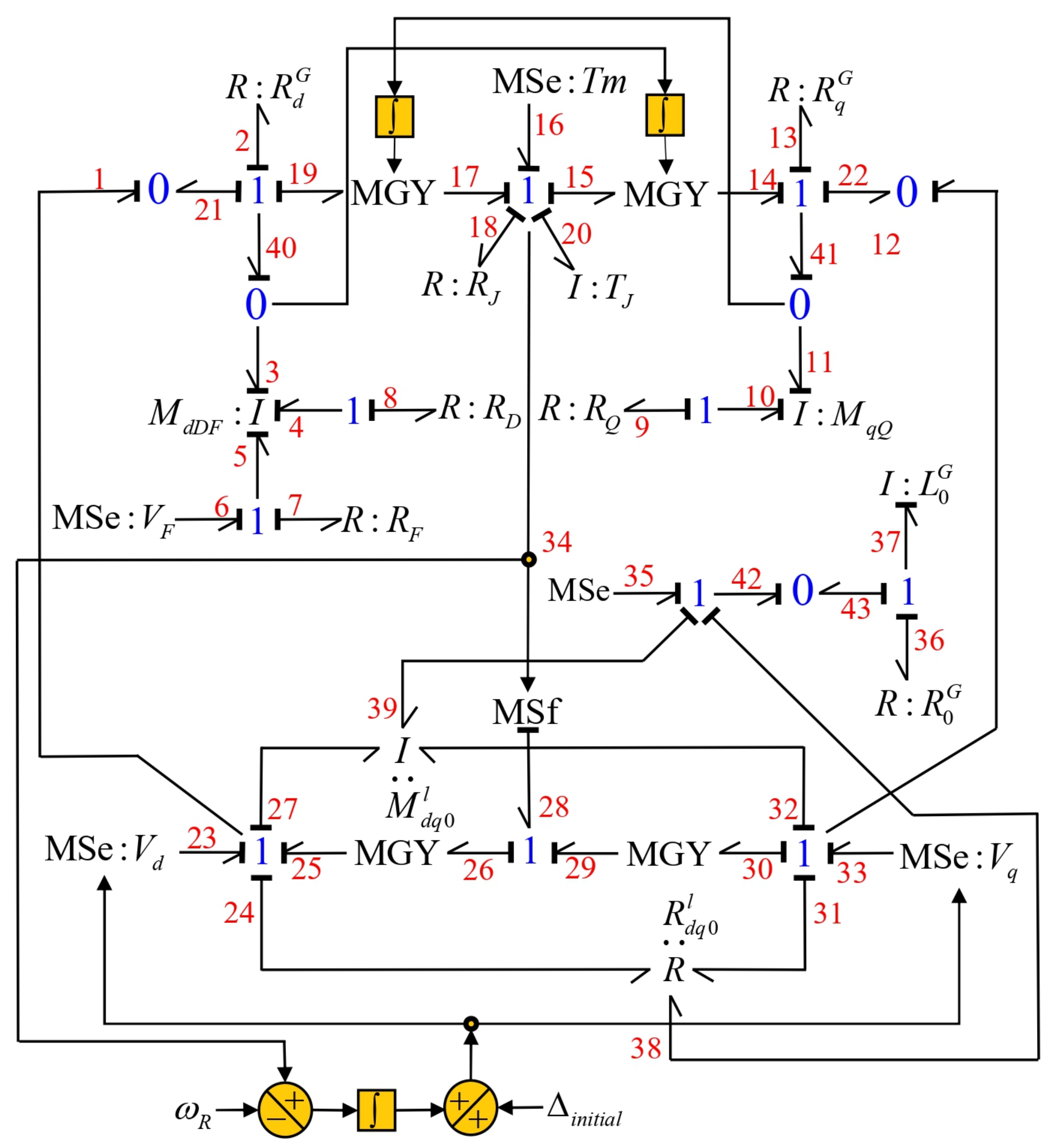
3.4. Case 4: Resistances and Inductances of the Non-Symmetrical Transmission Line

The most complicated case of a transmission line represents an unbalanced system, so the impedance matrices of the three-phase line in coordinates $\left(a,b,c\right)$ for inductance is (60) and for resistance is (71). In fact, this case is the simultaneous consideration of cases 1 and 2. Applying the Park transformation, the matrices in coordinates $\left(d,q,0\right)$ are given in (72) and (72). The BG for this case is shown in Figure 14.

The key vectors have already been defined in (40), the constitutive relations are described in (41) and (73) and the junction structure is given in (46). Therefore, the model in state space is a mixture of the matrices obtained in the previous cases; thus, $E\left(x\right)$ is given in (67), $A\left(x\right)$ in (79) and $B\left(x\right)$ is in (51), and the state space is expressed as

$$\begin{array}{ccc}\hfill \left[\begin{array}{ccccccc}\widehat{L_d}& M_{dD}& M_{dD}& M_{dq}& 0& M_{d0}& 0\\ M_{dD}& L_D& M_{DF}& 0& 0& 0& 0\\ M_{dD}& M_{DF}& L_F& 0& 0& 0& 0\\ M_{dq}& 0& 0& \widehat{L_q}& M_{qQ}& M_{q0}& 0\\ 0& 0& 0& M_{qQ}& L_Q& 0& 0\\ M_{d0}& 0& 0& M_{q0}& 0& \widehat{L_0}& 0\\ 0& 0& 0& 0& 0& 0& T_J\end{array}\right]\stackrel{•}{x}& =& \hfill \left[\begin{array}{ccccccc}-\widehat{R_d}& 0& 0& -R_{dq}& 0& -R_{d0}& -\widehat{{\lambda }_q^G}-{\lambda }_1\\ 0& -R_D& 0& 0& 0& 0& 0\\ 0& 0& -R_F& 0& 0& 0& 0\\ -R_{dq}& 0& 0& -\widehat{R_q}& 0& -R_{q0}& \widehat{{\lambda }_d^G}+{\lambda }_2\\ 0& 0& 0& 0& -R_Q& 0& 0\\ -R_{d0}& 0& 0& -R_{q0}& 0& -\widehat{R_0}& 0\\ \widehat{{\lambda }_q^G}& 0& 0& \widehat{{\lambda }_d^G}& 0& 0& -R_J\end{array}\right]x\hfill \\ & & \hfill +\left[\begin{array}{ccccc}-1& 0& 0& 0& 0\\ 0& 0& 0& 0& 0\\ 0& 0& 1& 0& 0\\ 0& -1& 0& 0& 0\\ 0& 0& 0& 0& 0\\ 0& 0& 0& 1& 0\\ 0& 0& 0& 0& 1\end{array}\right]u\hfill \end{array}$$

Once again, the BG of Figure 14 can be reduced to the BG shown in Figure 15.

The key vectors of this BG have been given in (40) with the storage elements of (76); then, the constitutive relations are described as (70) and (77). The junction structure for the submatrix $S_{11}$ is given by (63), the submatrices $S_{12}$ and $S_{21}$ are in (78), the submatrix $S_{13}$ is in (46) and $S_{22}=S_{23}=0$. Therefore, the matrix $E\left(x\right)$ is described in (67), and substituting (63) and (78) with (77) in (28), the state matrix is defined as

$$A\left(x\right)=\left[\begin{array}{ccccccc}-\widehat{R_d}& 0& 0& -R_{dq}& 0& -R_{d0}& -\widehat{{\lambda }_q}-{\lambda }_1\\ 0& -R_D& 0& 0& 0& 0& 0\\ 0& 0& -R_F& 0& 0& 0& 0\\ -R_{dq}& 0& 0& -\widehat{R_q}& 0& -R_{q0}& \widehat{{\lambda }_d}+{\lambda }_2\\ 0& 0& 0& 0& -R_Q& 0& 0\\ -R_{d0}& 0& 0& -R_{q0}& 0& -\widehat{R_0}& {\lambda }_3\\ \widehat{{\lambda }_q}& 0& 0& -\widehat{{\lambda }_d}& 0& 0& -R_J\end{array}\right]$$

(80)

and the input matrix is given by (51).

A physical representation of this case study with non-symmetrical resistances and inductances in the transmission line is shown in Figure 16.

Note that in this case, the SG can be seen with its nominal parameters in series with the parameters of the transmission line and some additional elements in the matrices $E\left(x\right)$ and $A\left(x\right)$, which are indicated with trajectories in blue and red in Figure 16.

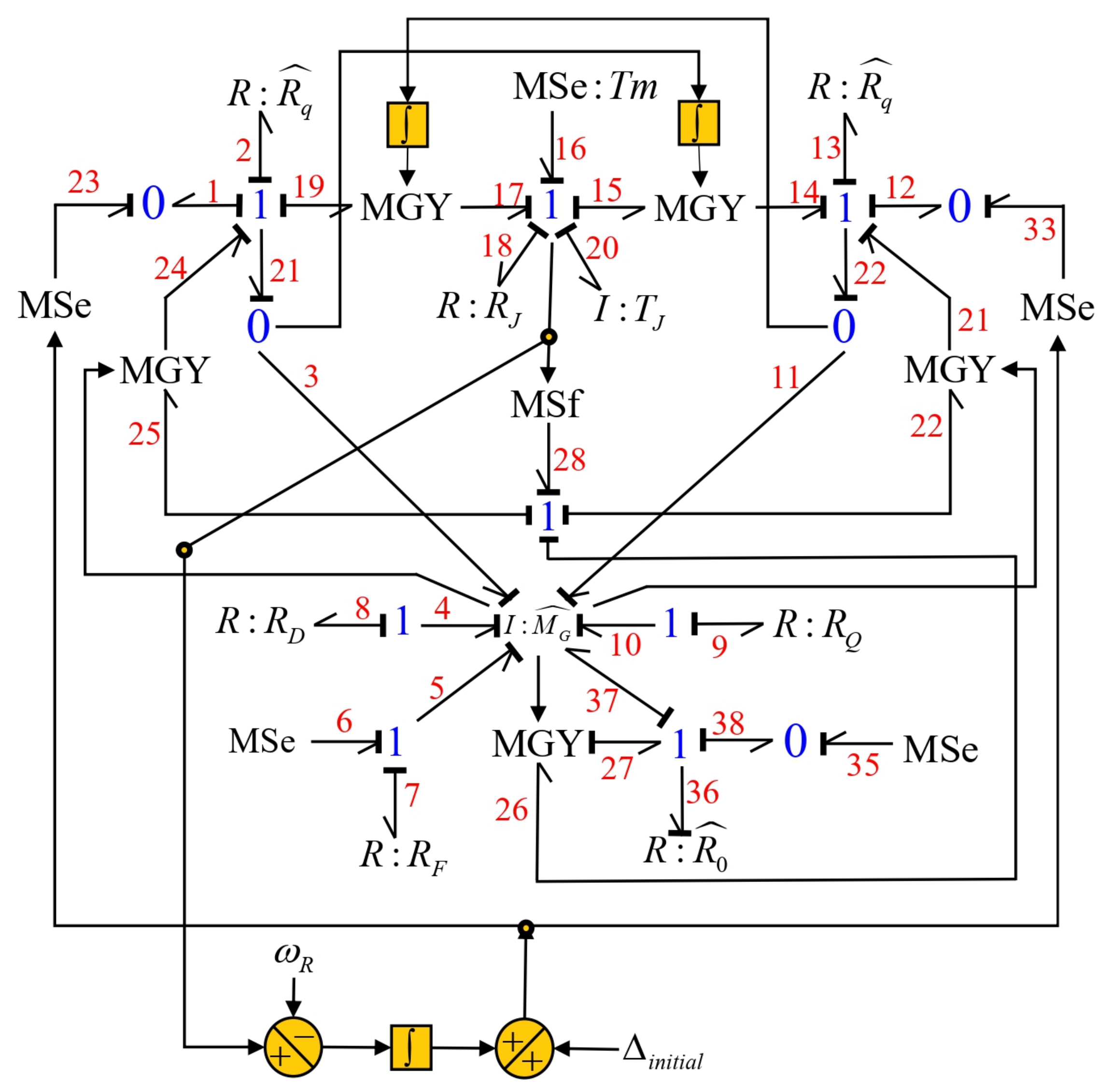
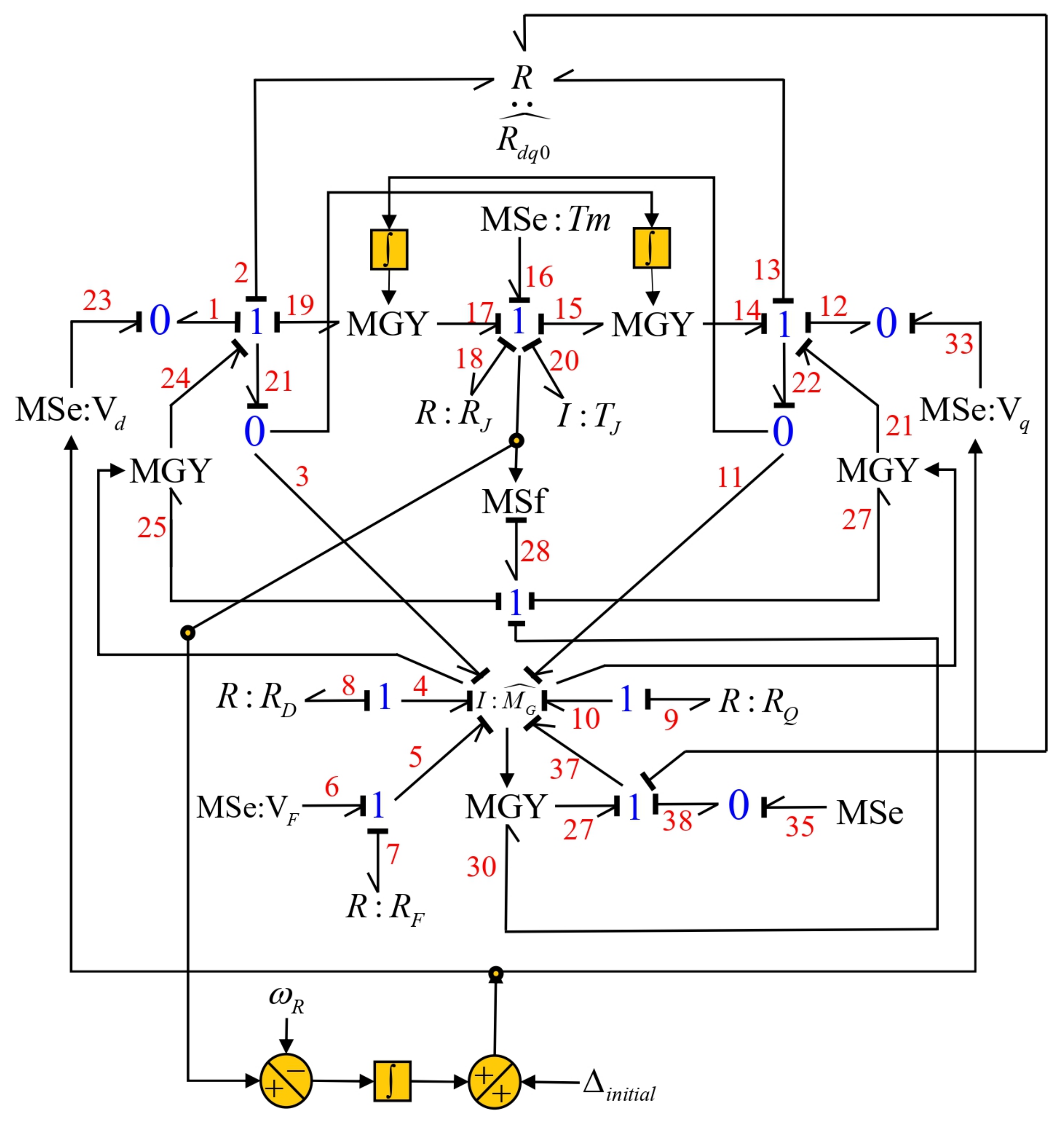
3.5. Novelty of the Proposed Reduction Method

Some contributions of this paper based on the reduction in the transmission line to the SG are given below:

• In the BG area:

  -

  The modeling of an SG connected to a transmission line and the infinite bus, showing how different schemes of the line can be obtained depending on its characteristics (symmetrical or non-symmetrical in resistance and/or inductance) and that independent elements of R or I, or R or I fields can be determined.

  -

  The transmission line is linearly dependent on the SG according to the causality of the storage elements.

  -

  The nonlinear terms of the system are clearly known with the gyrators modulated by state variables.

• In the field of electrical systems:

  -

  The influence of the flow links of the transmission line is known and determines a voltage drop in the R and I elements in each of the d, q and 0 axes.

  -

  The inductances of the transmission line are linearly dependent elements of the SG due to its derivative causality, which allows these inductances to be reduced.

  -

  When the transmission line is not symmetrical, there is a way to represent it with fields in BG, which, in the traditional approach, only determines equations.

  -

  The influence of each coordinate $\left(d,q0\right)$ of the SG and the transmission line with the model in BG is known.

  -

  For future work, the elements of the system can be modeled in more detail since in BG, we have each element individually and its implications in the complete system.

• In the areas of BG and electrical systems: the RBG proposal of the SG that includes the transmission line allows us to show how derivative causality can be included in the elements in integral causality; this causes model reduction and has computational advantages since derivative causality can cause problems in numerical simulation methods. The structure of the SG model in the reduced model with the line is preserved; there are only slight changes and these changes are only reflected in the coordinates $\left(d,q\right)$ of the SG, while the field winding, damping windings and mechanical subsystem do not require any change.

The method to obtain the BG from the complete BG is described below.

• The BG model of the SG of the system connected to the infinite bus retains the same structure, that is, all its bonds and elements are maintained.
• The values of the resistances and inductances of the SG are the sums of the resistances and inductances of the SG and the transmission line in each axis: d, q and 0.
• For the case of a non-symmetrical transmission line, new causal trajectories are added that are formed in the following way:

  -

  It starts from a modulated flow source $M{S}_f$ whose value is the velocity of the SG and this is obtained from an active bond of 1-junction of the mechanical subsystem.

  -

  The source bond enters a modulated gyrator with a value that is the flux link corresponding to the transmission line gyrator of the complete BG.

  -

  The output bond of the gyrator is connected to 1-junction of the axis $\left(d,q0\right)$ that corresponds to it.

  -

  The I-fields of the SG are changed for a single I-field, whose constitutive relationship is defined by the matrix $E\left(x\right)$.

The objective of obtaining the mathematical models of the complete BG and the RBG is to verify that they represent the same system.

The behavior of the synchronous generator in the different cases is simulated in the following section.

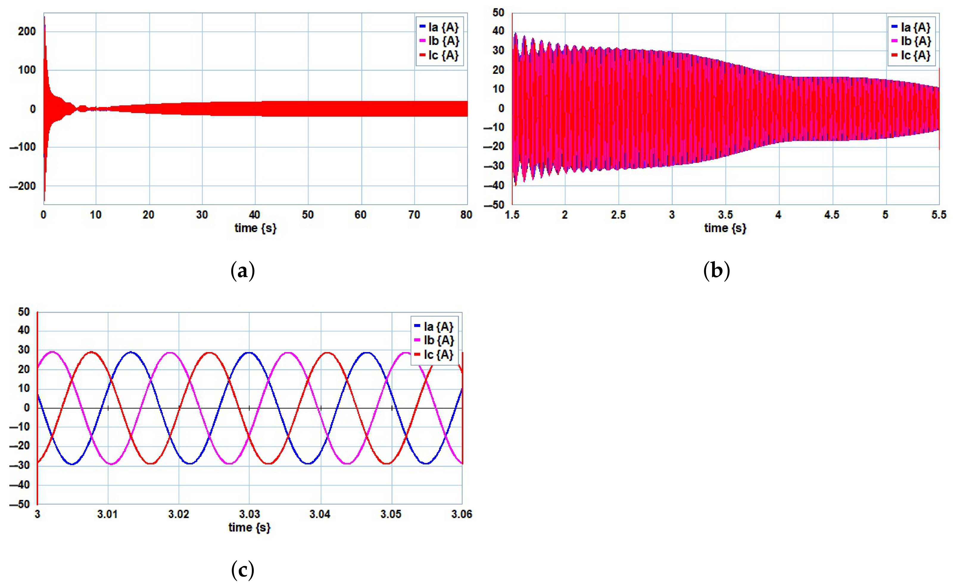
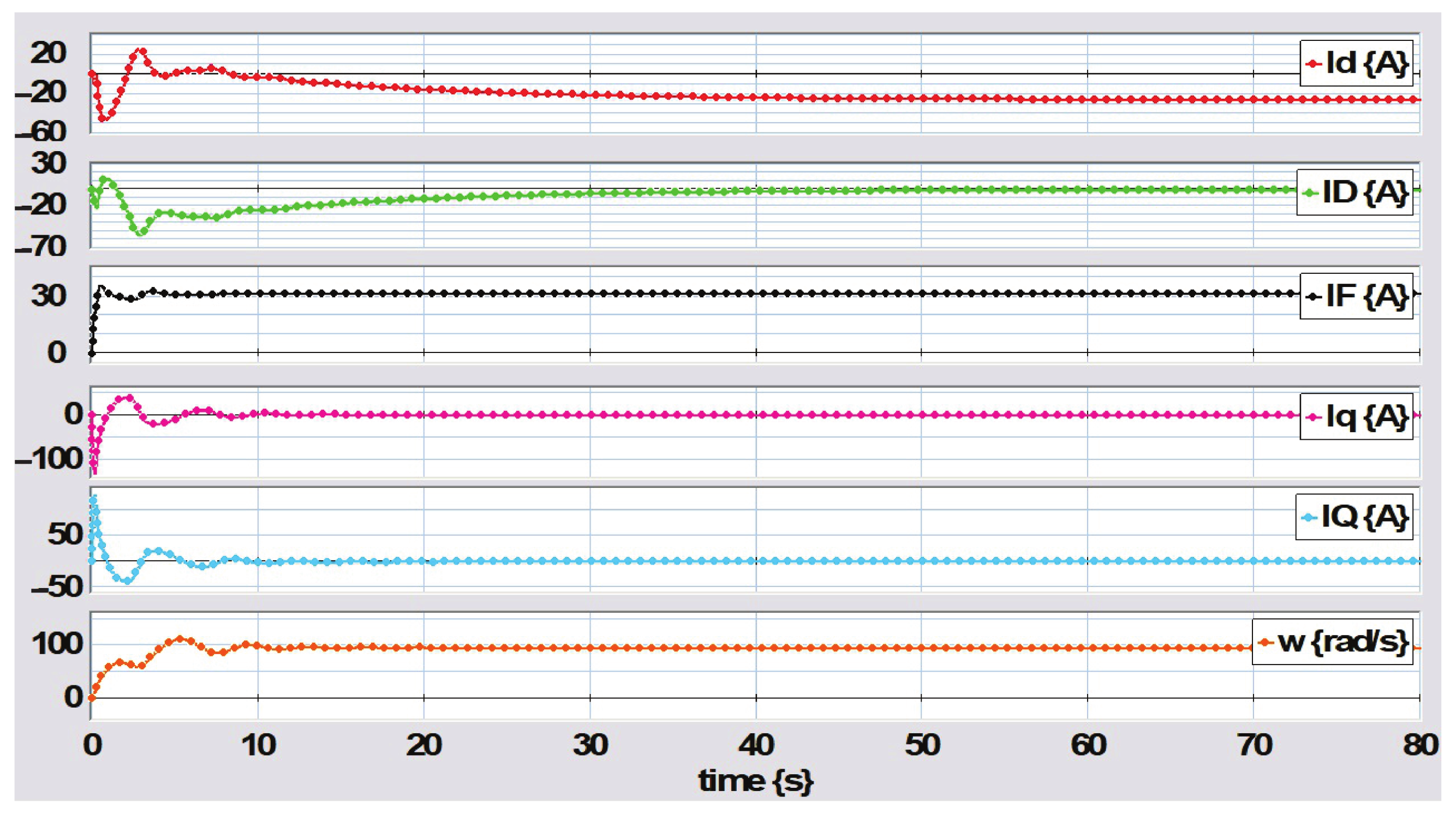
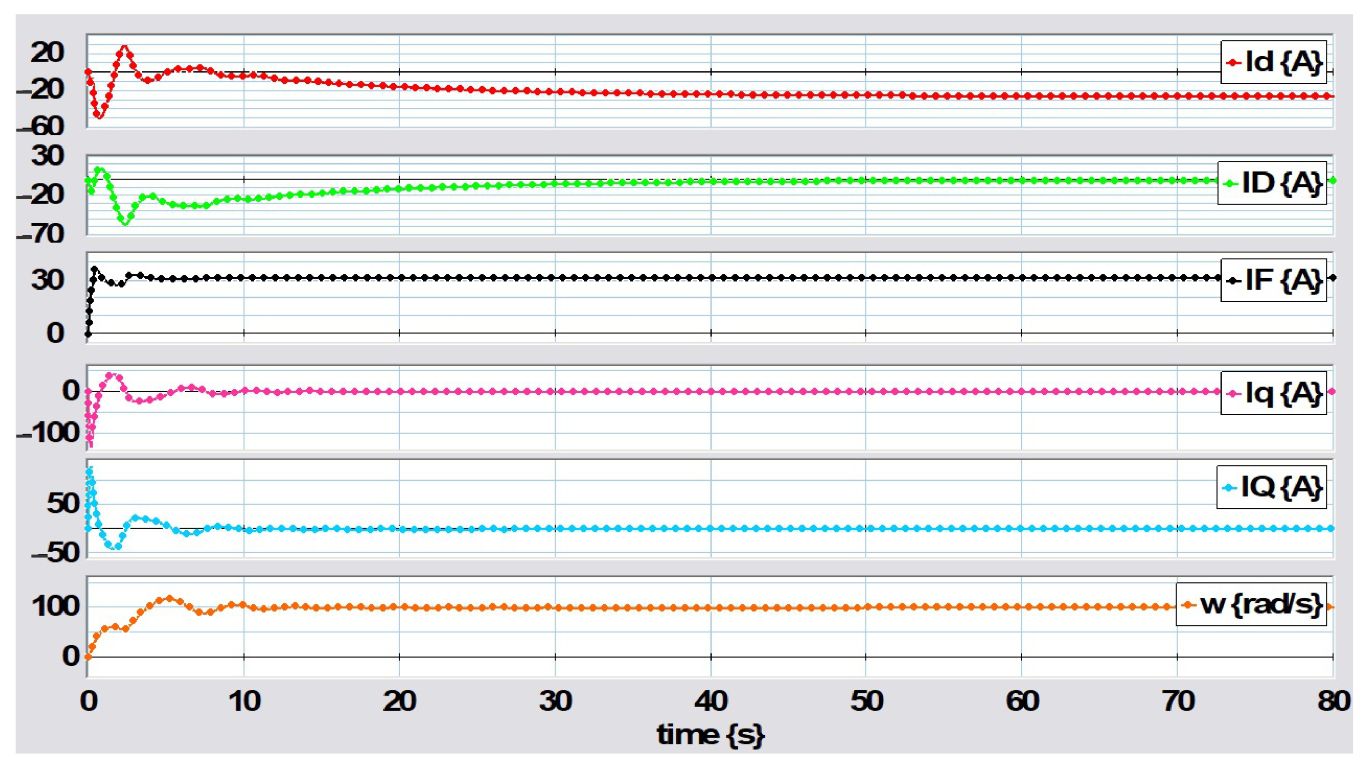
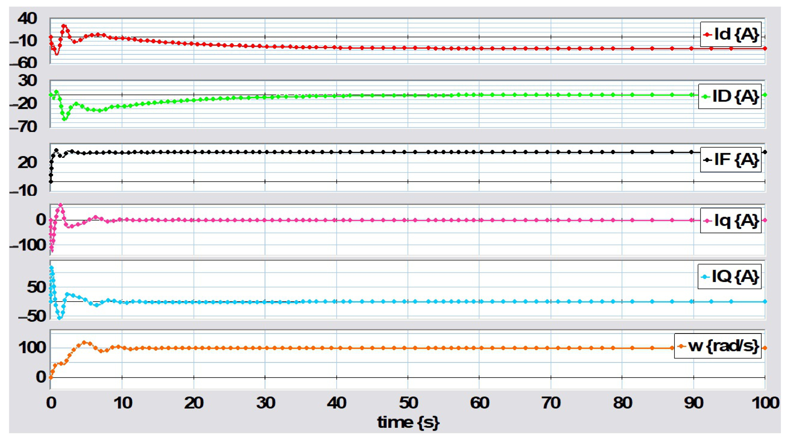
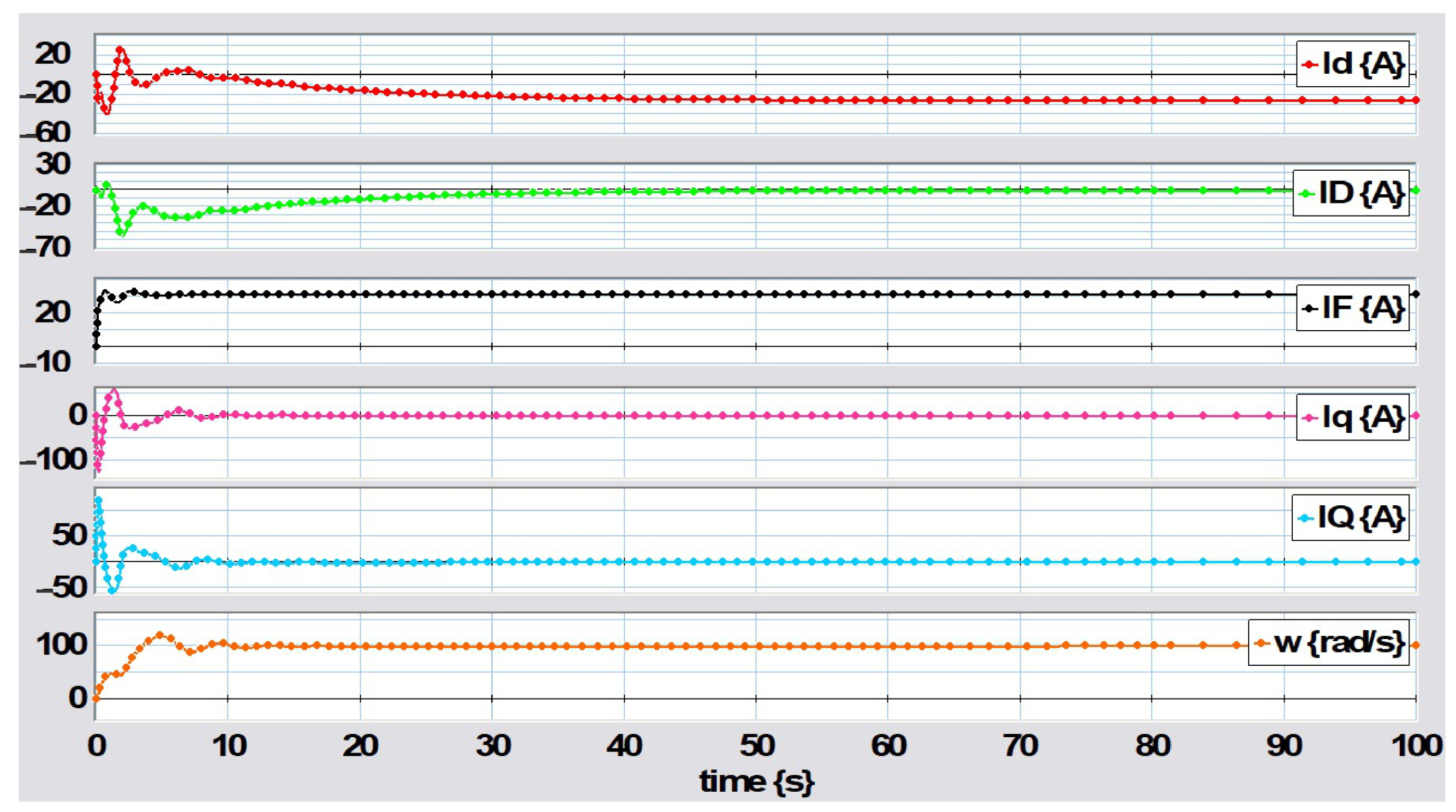
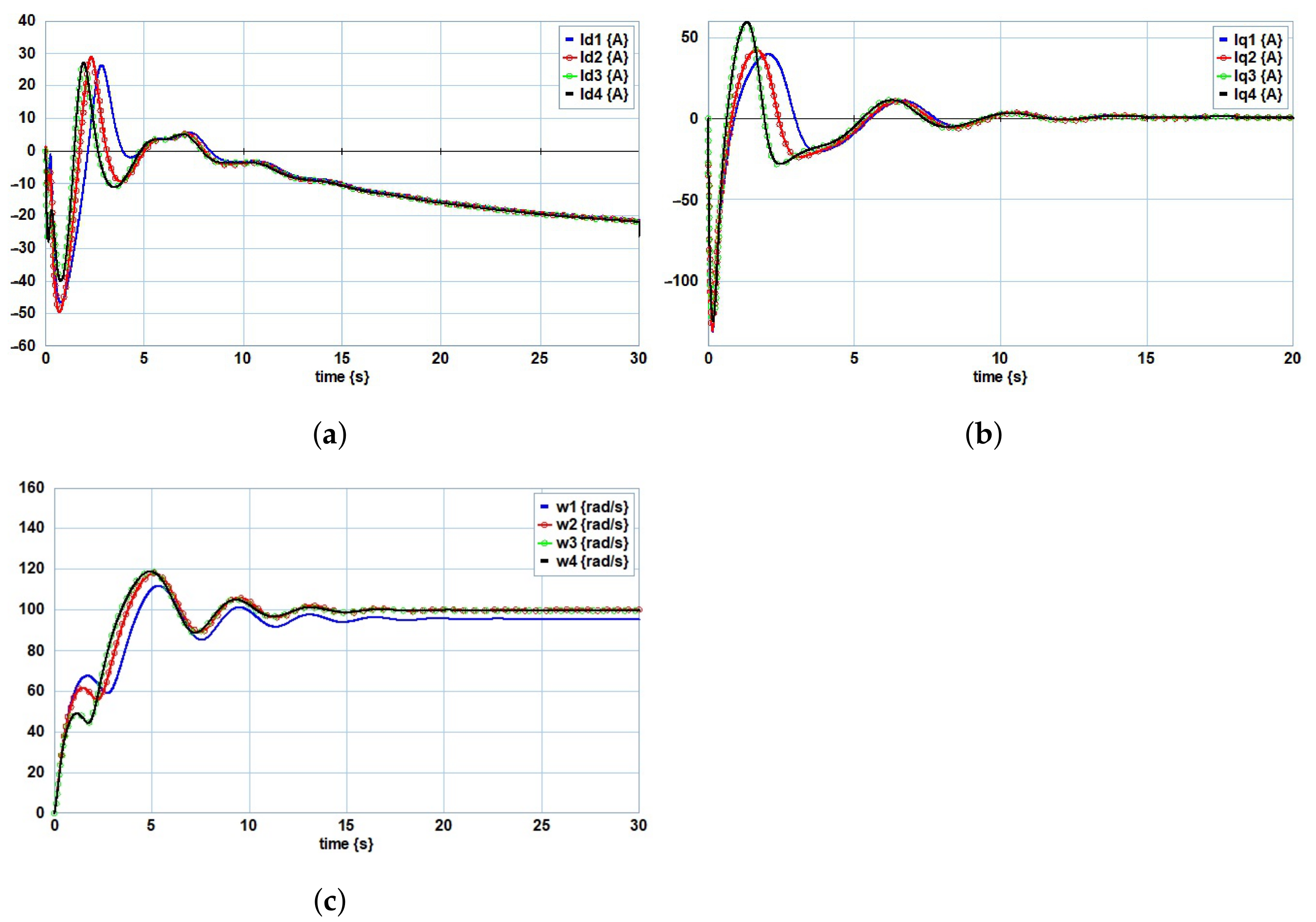
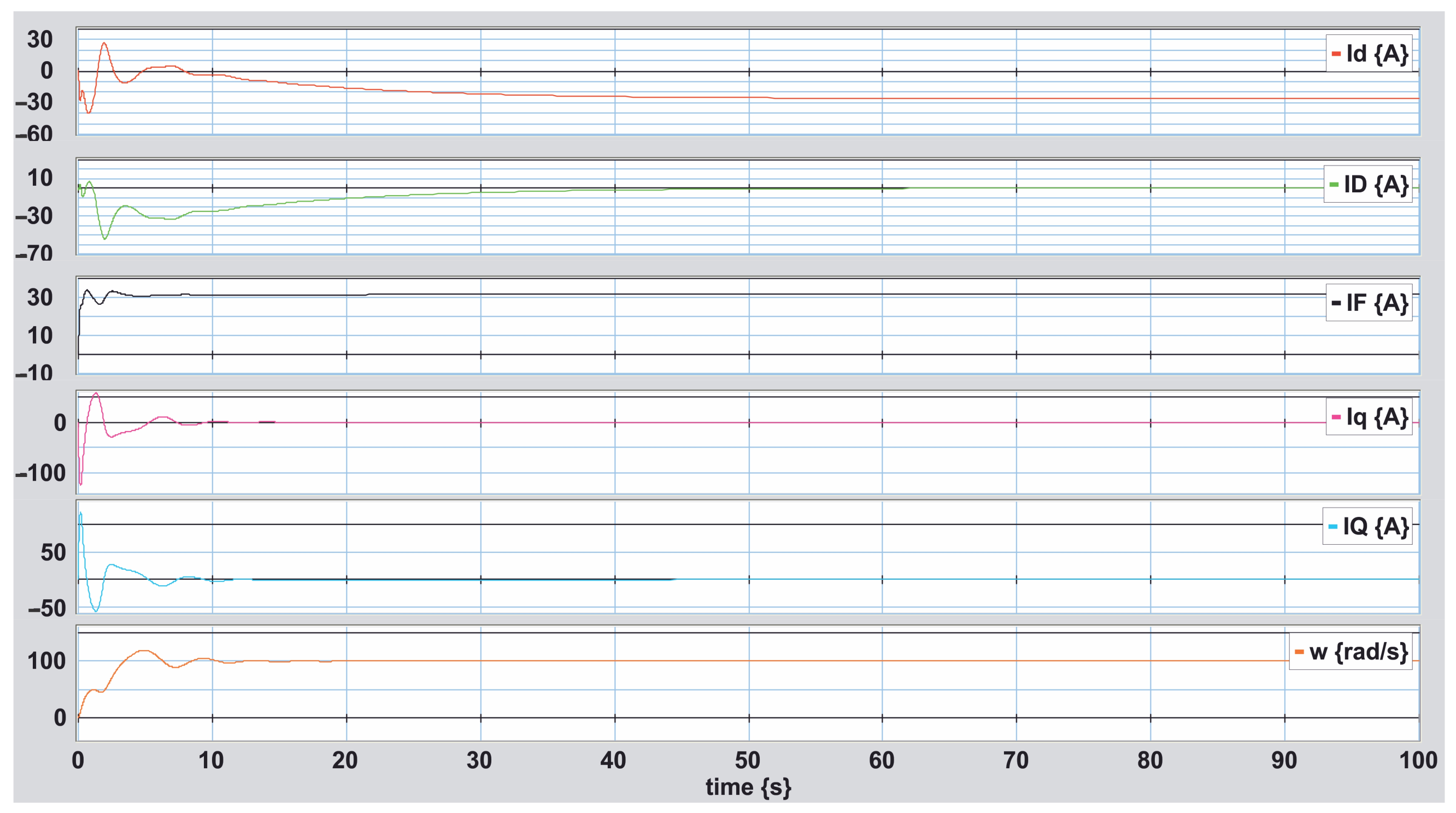
4. Simulation Results

Once the symbolic expressions of the four case studies of the SG connection to an infinite bus have been obtained from their BG models, it is pertinent to simulate these cases using the 20-Sim software (version 4.1).The numerical parameters of the SG are given in

Table 1. SG parameters.

${\mathit{v}}_{\mathit{a}}=220sin\left(\mathit{w}\mathit{t}\right)$ V	${\mathit{R}}_{\mathit{d}}^{\mathit{G}}=0.5\mathsf{\Omega }$	${\mathit{L}}_{\mathit{d}}^{\mathit{G}}=1.7$ H	${\mathit{M}}_{\mathit{d}\mathit{D}}=1.55$ H
$v_b=220sin\left(wt-2\pi /3\right)$ V	$R_q^G=0.5\mathsf{\Omega }$	$L_q^G=1.64$ H	$M_{qQ}=1.49$ H
$v_c=220sin\left(wt+2\pi /3\right)$ V	$R_0^G=0.5\mathsf{\Omega }$	$L_0^G=1.0$ H	$M_{dF}=1.55$ H
$v_F=30$ V	$R_F=0.95\mathsf{\Omega }$	$L_D=1.605$ H	$M_{DF}=1.55$ H
$T_m=100$ N· m	$R_J=1.0$ N· m· s	$L_Q=1.526$ H	$T_J=2.37$ N· m· s2

.

In order to provide the necessary tools to interpret the BGs for simulation purposes, a flow chart is illustrated in Figure 17.

The behavior of the SG connected directly to the infinite bus is illustrated in Figure 18.

The variables shown in Figure 18 are the currents in coordinates $\left(d,q\right)$ of the stator $i_d$ and $i_q$, respectively; the currents are stable. The currents in the damping windings $i_D$ and $i_Q$ after the electromechanical transient stabilize at zero as expected. The current in the field winding $i_F$ after the transient period due to the start-up process stabilizes at the value of $V_F/R_F$. The velocity of the SG after a soft transient stabilizes, having the desired behavior.

The profile of the currents generated in coordinates $\left(a,b,c\right)$ is shown in Figure 19. They are shown on different time scales where you can observe the evolution of the symmetrically distributed three-phase currents; and at the end of the transient period, the behavior of the currents are in a stable manner.

Connecting the transmission line to the SG-infinite bus link that determines case 1, the parameters of the line are

$$\begin{array}{ccc}\hfill R_d^l& =& \hfill R_q^l=R_0^l=2.5\mathsf{\Omega }\hfill \end{array}$$

(81)

$$\begin{array}{ccc}\hfill L_d^l& =& \hfill L_q^l=L_0^l=0.001\mathrm{H}\hfill \end{array}$$

(82)

There is a balanced transmission line and the behavior of the SG variables is illustrated in Figure 20.

Applying case 2, that is, the transmission line has balanced resistances given by (81), but the inductances are unbalanced and are given by

$$M_{dq0}=\left[\begin{array}{ccc}0.001& 0.0005& 0.0005\\ 0.0005& 0.001& 0.0005\\ 0.0005& 0.0005& 0.001\end{array}\right]H$$

(83)

The behavior of the generator in this operating condition is shown in Figure 21.

Considering balanced inductances of the line given by (82) and the line resistances unbalanced

$$R_{dq0}=\left[\begin{array}{ccc}4.9803& -2.2301& -0.2168\\ -2.2301& 6.3529& 3.2927\\ -0.2168& 3.2927& 5.6666\end{array}\right]\mathsf{\Omega }$$

(84)

which determines case 3 and whose generator behavior is shown in Figure 22.

Considering an unbalanced transmission line whose values are indicated in (83) and (84), the behavior of the SG is illustrated in Figure 23.

The comparison of the four case studies is illustrated in Figure 24. The currents in the d and q axes of the four cases $\left(i_{d1},i_{d2},i_{d3},i_{d4}\right)$ and $\left(i_{q1},i_{q2},i_{q3},i_{q4}\right)$ are shown in Figure 24a,b, respectively. The velocity of each case $\left(w_1,w_2,w_3,w_4\right)$ is illustrated in Figure 24c.

The steady state values of the variables shown in Figure 24 are indicated in

Table 2. Steady state values for the four case studies.

	${\mathit{I}}_{\mathit{d}}\left(\mathit{A}\right)$	${\mathit{I}}_{\mathit{q}}\left(\mathit{A}\right)$	${\mathit{I}}_{\mathit{D}}\left(\mathit{A}\right)$	${\mathit{I}}_{\mathit{Q}}\left(\mathit{A}\right)$	${\mathit{I}}_{\mathit{F}}\left(\mathit{A}\right)$	w (rad/s)
Case 1	$-25.8734$	$0.1168$	$-0.09467$	$-0.0290$	$31.5778$	$95.5998$
Case 2	$-26.0851$	$0.02191$	$-0.0193$	$-0.02671$	$31.5787$	$100.0006$
Case 3	$-26.1411$	$0.0212$	$-0.0184$	$-0.02586$	$31.5787$	$100.0005$
Case 4	$-26.1437$	$0.0211$	$-0.0183$	$-0.0257$	$31.5787$	$100.0004$

.

Now, the losses that occur in the system are given in terms of efficiency in the following way. For case 1, the efficiency is

$$n_1=72.2213\%$$

for case 2

$$n_2=70.0136\%$$

for case 3

$$n_3=70.0025\%$$

and for case 4

$$n_4=70.0217\%$$

Note that the steady state values and efficiencies are very close because the values of the symmetrical and non-symmetrical transmission lines are close.

If one should want to experimentally verify the results given in this paper, knowing the parameters of an SG, one should connect the transmission line with values in such a way that the same values of this paper or other study’s case result are used.

The simulation results of references [1,2,3] show that the behavior of the complete system is close to those presented in this paper, with different magnitudes due to the difference in the parameters. Furthermore, the state space representation of the BGs of the complete system and the RBGs indicate the validity of the behavior of the machine variables.

Although the simulation results using a BG can be obtained with traditional power system methods, the BG allows for making some change in the connection, presents the introduction of new elements (unmodeled dynamics) or failures of some element, and causes the simulation results to be performed directly.

The behavior of the different cases is similar, because the SG is robust enough to withstand changes in the parameters and characteristics of the transmission line. However, in simulating case study 3, there are equal transmission line inductances in the three phases, but the line resistances are given by

$$R_{abc}^l=\left[\begin{array}{ccc}100& 0& 0\\ 0& 50& 0\\ 0& 0& 200\end{array}\right]\mathsf{\Omega }$$

(85)

in coordinates $\left(d,q,0\right)$

$$R_{dq0}^l=\left[\begin{array}{ccc}88.1961& 33.6730& -50.1633\\ 33.6730& 145.1372& -37.0476\\ -50.1633& -37.0476& 116.6666\end{array}\right]\mathsf{\Omega }$$

(86)

The result of the simulation of the generator variables is illustrated in Figure 25.

Note that this case is a limit for the behavior of the SG that, due to the resistance in the transmission line, causes unstable behavior, which is not desirable. Although this operating condition is not common, it can occur in a failure condition due to some situation in the transmission line.

It is important to mention that the simulations presented in this section are intended to describe the behavior of the system, and this can be obtained by modeling the electrical power system with traditional methods. Furthermore, the richness of the BG is that a model is determined from an analysis and that the reduced models give an alternative of incorporating the transmission line within the generator as well as how this line changes to the SG and how it is reflected in its elements.

As future work, other more complex configurations of transmission lines can be connected to the synchronous generator and the direct implications on the generator in the physical domain can be analyzed.

5. Conclusions

The BG modeling of an SG connected to an infinite bus through a transmission line has been presented. Because the transmission line can be symmetrical or non-symmetrical in its resistance and inductance, four case studies have been proposed. If it is symmetrical with the same resistance and inductance values of the three phases, the BG model has individual elements for its resistance and inductance.When the line is not symmetrical in resistance and/or inductance, the models in the BG are given in fields-R and/or fields-I in coordinates $\left(d,q,0\right)$. Due to the derivative causality of the transmission line inductances, these are linearly dependent on the SG inductances; therefore, reduced models can be obtained. RBG models for the four case studies are proposed. These RBG models have the characteristics of practically presenting the model of the SG with some additional elements and some of the values of its elements are modified. Therefore, these RBG models indicate how the SG can include the transmission line within it. It is common that the bond graph methodology does not directly see the equations that describe the system, so a junction structure of the electrical system modeled in a bond graph that determines its mathematical model in state space is proposed. Simulation results are shown for the four case studies. The currents in the d and q axes for the case of a symmetrical line are 25.87 A and 0.1168 A, and for a non-symmetrical line in resistance and inductance are −26.14 A and 0.0211 A; these values are close because the imbalance is not very large. With a high imbalance, there is a condition of SG instability, which is given in the paper. This paper presents the beginning of future work, for example, the modeling of transmission lines with distributed parameters or $\pi$ circuits, as well as the modeling and analysis of an SG, transmission line and induction motors, and finally, the determination of the stability of the SG with a transmission line.

References

- Anderson, P.M. Power System Control and Stability; The Iowa State University Press: Ames, IA, USA, 1977. [Google Scholar]
- Kundur, J.R. Power System Stability and Control; Mc. Graw-Hill: New York, NY, USA, 1994. [Google Scholar]
- Krause, P.C.; Wasynczuk, O.; Sudhoff, S.D. Analysis of Electrical Machinery and Drive Systems; IEEE Press, Wiley-Interscience: Piscataway, NJ, USA, 2002. [Google Scholar]
- Demiroren, A.; Zeynelgil, H.L. Modelling and simulation of synchronous machine transient analysis using SIMULINK. Int. J. Electr. Eng. Educ. 2002, 39, 337–346. [Google Scholar] [CrossRef]
- Unamuno, E.; Suul, J.A.; Molinas, M.; Barrena, J.A. Comparative Eigenvalue Analysis of Synchronous Machine Emulations and Synchronous Machines. In Proceedings of the IECON 2019-45th Annual Conference of the IEEE Industrial Electronics Society, Lisbon, Portugal, 14–17 October 2019; pp. 3863–3870. [Google Scholar]
- Safar, H. Power Transmission Line Analysis Using Exact, Nominal, and Modified Models. In Proceedings of the 2nd International Conference on Computer and Automation Engineering (ICCAE), Singapore, 26–28 February 2010; pp. 128–134. [Google Scholar]
- Oliveira, L.M.R.; Cardoso, A.J.M. Modelling and Simulation of Three-Phase Power Transformers. In Proceedings of the 6th International Conference on Modelling and Simulation of Electrical Machines, Converters and Systems, (ELECTRIMACS 99), Lisbon, Portugal, 14–16 September 1999; pp. 257–262. [Google Scholar]
- Milanovic, J.V.; Hiskens, I.A. Oscillatory interaction between synchronous generator and local voltage-dependent load. IEE Proc.-Gener. Transm. Distrib. 1995, 142, 473–480. [Google Scholar] [CrossRef]
- Jain, H.; Parchure, A.; Broadwater, R.P.; Dilek, M.; Woyak, J. Three-Phase Dynamic Simulation of Power Systems Using Combined Transmission and Distribution System Models. IEEE Trans. Power Syst. 2016, 31, 4517–4524. [Google Scholar] [CrossRef]
- Lu, S.; Zhu, Y.; Dong, L.; Na, G.; Hao, Y.; Zhang, G.; Zhang, W.; Cheng, S.; Yang, J.; Sui, Y. Small- Signal Stability Research of Grid-Connected Virtual Synchronous Generators. Energies 2022, 15, 7158. [Google Scholar] [CrossRef]
- Chennakesavan, C.; Nalandha, P. Multi-Machine Small Signal Stability Analysis for Large Scale Power System. Indian J. Sci. Technol. 2014, 7, 40–47. [Google Scholar] [CrossRef]
- Obe, E.S. Small Signal Analysis of Load Angle Governing and Excitation Control of AC Generators. Niger. J. Technol. 2005, 24, 19–33. [Google Scholar]
- Bellan, D. Analytical Investigation of the Properties of Transients in Unbalanced Three-Phase Four-Wire Networks. Energies 2022, 15, 9122. [Google Scholar] [CrossRef]
- Qin, X.; Liu, N.; Zhao, L. Study on the Physical Mechanism and the Fast Algorithm of ATC Constrained by Transient Stability for the Point- to- grid Transmission System. In Proceedings of the 2015 IEEE Power & Energy Society General Meeting, Denver, CO, USA, 26–30 July 2015. [Google Scholar]
- Chavez, J.J.; Madrigal, M.; Dinavahi, V. Real-Time Simulation of Three-Phase Transmission Lines Modeled in the Dynamic Harmonic Domain. In Proceedings of the International Conference on Power Systems Transients (IPST 2011), Delf, The Netherlands, 14–17 June 2011. [Google Scholar]
- Xu, H.; Zhang, R.; Li, X.; Yan, Y. Fault Tripping Criteria in Stability Control Device Adapting to Half-Wavelenght AC Transmission Line. IEEE Trans. Power Deliv. 2019, 14, 1619–1625. [Google Scholar] [CrossRef]
- Chaban, A.; Lis, M.; Szafraniec, A.; Levoniuk, V. Mathematical Modelling of Transient Processes in a Three Phase Electric Power System for a Single Phase Short-Circuit. Energies 2022, 15, 1126. [Google Scholar] [CrossRef]
- Elmetwaly, A.H.; ElDesouky, A.A.; Omar, A.I.; Saad, M.A. Operation control, energy management, and power quality enhacement for a cluster of isolated microgrids. Ain Shams Eng. J. 2022, 13, 101737. [Google Scholar] [CrossRef]
- Kermani, M.; Adelmanesh, B.; Shirdare, E.; Sima, C.A.; Carni, D.L.; Martirano, L. Intelligent energy management based on SCADA system in a real Microgrid for smart building applications. Renew. Energy 2021, 171, 1115–1127. [Google Scholar] [CrossRef]
- Subramanian, D.P.; Harinee, K. Small Signal Stability Analysis of Multi-Machine Power Systems Interfaced with Micro Grid. Int. J. Eng. Res. Technol. (IJERT) 2014, 3, 299–306. [Google Scholar]
- Izumi, S.; Karakawa, Y.; Xin, X. Analysis of samll-signal stability of power systems with photovoltaic generators. Electr. Eng. 2019, 101, 321–331. [Google Scholar] [CrossRef]
- Benedetti, L.; Papadopoulos, P.N.; Alvarez, A.E. Small Signal Interactions Involving a Synchronous Machine and a Grid Forming Converter. In Proceedings of the 2021 IEEE Madrid PowerTech, Madrid, Spain, 28 June–2 July 2021. [Google Scholar]
- Firdaus, A.; Anwar, A. Effect of Alternator’s Inertia Constant H on Small Signal Oscillations in Power System. Int. J. Electron. Electr. Eng. 2014, 7, 567–572. [Google Scholar]
- Chu, T.; Xu, M.; Wang, S.; Li, D.; Liu, G. Small-Signal Stability Analysis of the Power System Based on Active Support of REnewable Energy VSCs. Front. Energy Res. 2022, 10, 907790. [Google Scholar] [CrossRef]
- Ding, L.; Liu, X.; Tan, J. Small-Signal Stability Analysis of Low- Inertia Power Grids with Inverter-Based Resources and Synchronous Condensers. In Proceedings of the IEEE PES Innovative Smart Grid Technologies Conference (ISGT NA), New Orleans, LA, USA, 21–24 February 2022. [Google Scholar]
- Shivam, G.; Kumar, T.D. Modelling and Simulation of 3-Phase Grid connected Solar PV System with Power Quality Analysis. Res. Quantum Comput. Phys. Syst. 2018, 1, 1–5. [Google Scholar]
- Mayoral, E.H.; Reyes, E.D.; Cortez, R.I.; Mercado, E.C.; Garcia, V.T.; Gosebruch, R.U. Modeling and Validation of the Switching Techniques Applied to Back-to-Back Power Converter Connected to a DFIG-Based Wind Turbine for Harmonic Analysis. Electronics 2021, 10, 3046. [Google Scholar] [CrossRef]
- Costa, I.D.L.; Brandao, D.I.; Junior, L.M.; Simoes, M.G.; Morais, L.M.F. Analysis of Stationary- and Synchronous- Reference Frames for Three-Phase Three-Wire Grid-Connected Converter AC Current Regulators. Energies 2021, 14, 8348. [Google Scholar] [CrossRef]
- Karnopp, D.C.; Rosenberg, R.C. Systems Dynamics: A Unified Apprach; Wiley John & Sons: Hoboken, NJ, USA, 2000. [Google Scholar]
- Gawthrop, P.; Smith, L. Metamodelling; Prentice-Hall: Hoboken, NJ, USA, 1989. [Google Scholar]
- Brown, F.T. Engineering System Dynamics; Dekker: New York, NY, USA, 1989. [Google Scholar]
- Dauphin-Tanguy, G. Les Bond Graphs; Hermes Science Europe: London, UK, 2000. [Google Scholar]
- Thoma, J.; Bouamama, B.O. Modelling and Simulation in Thermal and Chemical Engineering a Bond Graph Approach; Springer: Berlin/Heidelberg, Germany, 2000. [Google Scholar]
- Dauphin-Tanguy, G.; Rahmani, A.; Sueur, C. Bond graph aided design of controlled systems. Simul. Pract. Theory 1999, 7, 493–513. [Google Scholar] [CrossRef]
- Brown, F.T. Hamiltonian and Lagrangian Bond Graphs. J. Frankl. Inst. 1991, 328, 809–831. [Google Scholar] [CrossRef]
- Xu, J.; Yan, H.; Liu, S.; Zhang, Y.; Tan, W. Bond Graph-Based Approach to Modeling Variable-Speed Gearboxes with Multi-Type Clutches. Appl. Sci. 2022, 12, 6181. [Google Scholar] [CrossRef]
- Phillips, J.R.; Amirouche, F. Bond-graph Representation of Ideal Constraints via the Principle of Virtual Power. ECCOMAS Thematic. In Proceedings of the Conference on Multibody Dynamics, Lisbon, Portugal, 24–28 June 2023. [Google Scholar]
- Zrafi, R.; Ghedira, S.; Besbes, K. A Bond Graph Approach for the Modeling and Simulation of a Buck Conerter. J. Low Power Electron. Appl. 2018, 8, 2. [Google Scholar] [CrossRef]
- Mahmoudi, A.; Roshandel, E.; Kahourzade, S.; Vakilipoor, F.; Drake, S. Bond graph model of line-start permanent-magnet synchronous motors. Electr. Eng. 2024, 106, 1667–1681. [Google Scholar] [CrossRef]
- Badoud, A.E.; Merahi, F.; Bouamama, B.O.; Mekhilef, S. Bond Graph modeling, design and experimental validation of a photovoltaic/ fuel cell/ electrolyzer/ battery hybrid power system. Int. J. Hydrogen Energy 2021, 46, 24011–24027. [Google Scholar] [CrossRef]
- Vali, S.H.; Kiranmayi, R. Design of Zero Voltage Switching Boost DC-DC Converter Using Bond Graph Model. EMITTER Int. Eng. Technol. 2020, 8, 426–441. [Google Scholar] [CrossRef]
- Mohammed, A.; Sirahbizu, B.; Lemu, H.G. Optimal Rotary Wind Turbine Blade Modeling with Bond Graph Approach for Specific Local Sites. Energies 2022, 15, 6858. [Google Scholar] [CrossRef]
- Fang, Z.; Wang, J.; Xiong, F.; Xie, X. Research on the dynamic characteristics of the acquisittion mechanism of the oscillating flapping wing wave energy power generation device based on the bond graph. J. Phys. 2021, 2125, 012050. [Google Scholar]
- Sahm, D. A two-axis bond graph model of the dynamics of synchronous electrical machine. J. Frankl. Inst. 1979, 308, 205–218. [Google Scholar] [CrossRef]
- Hernandez, I.N.; Breeveld, P.C.; Weustink, P.B.T.; Gonzalez, G. A phasor analysis of a synchronous generator: A bond graph approach. Int. J. Electr. Comput. Electron. Commun. Eng. 2014, 8, 1086–1092. [Google Scholar]
- Gonzalez, G.; Barrera, N.; Ayala, G.; Padilla, J.A.; Alvarado, D. Dynamic performance of a Skystream wind turbine: A bond Graph approach. Cogent Eng. 2019, 6, 1709361. [Google Scholar] [CrossRef]
- Gonzalez, G.; Ayala, G.; Barrera, N.; Padilla, J.A. Linearization of a class of non-linear systems modelled by multibond graphs. Math. Comput. Model. Dyn. Syst. 2019, 25, 284–332. [Google Scholar] [CrossRef]
- Gonzalez, G.; Barrera, N.; Ayala, G.; Padilla, J.A. Modeling and Simulation in Multibond Graphs Applied to Three-Phase Electrical Systems. Appl. Sci. 2023, 13, 5880. [Google Scholar] [CrossRef]
- Kadiman, S.; Yuliani, O. Comparison performance study of singly-fed and doubly-fed induction generators-based bond graph wind turbines model. Int. J. Electr. Comput. (IJECE) 2024, 14, 3592–3606. [Google Scholar] [CrossRef]
- Boum, A.T.; Tatchou, D.G. Modeling, Simulation and Fault Diagnosis of a Doubly Fed Induction Generator using Bond Graph. Int. J. Control. Syst. Robot. 2020, 5, 34–40. [Google Scholar]
- Hamza, W.; Jamel, B.S.; Najeh, L.M. Application of Bond Graph of Renewable Energy Sources in Smart Grids. J. Electr. Electron. Eng. 2020, 13, 97–102. [Google Scholar]
- Mezghani, D.; Mami, A.; Dauphin-Tanguy, G. Bond graph modelling and control enhacement of an off-grid hybrid pumping system by frequency optimization. Int. J. Numer. Model. Electron. Netw. Devices Fields 2020, 33, e2717. [Google Scholar] [CrossRef]
- Lenz, R.; D-Olek, A.; Kugi, A.; Kemmetmuller, W. Optimal fault-tolerant control with radial force compensation for multiple open-circuit faults in multiphase PMSMs - A comparison of n-phase and multiple three-phase systems. Control Eng. Pract. 2024, 147, 105924. [Google Scholar] [CrossRef]
- Musca, R.; Longatt, F.G.; Sanchez, C.G. Power System Oscillations with Different Prevalence of Grid-Following and Grid-Forming Converters. Energies 2022, 15, 4273. [Google Scholar] [CrossRef]
- Smadi, I.A.; Ibrahim, I.E.A.A.A. An Improved Delayed Signal Cancelation for Three-Phase Grid Synchronization with DC Offset Immunity. Energies 2023, 16, 2873. [Google Scholar] [CrossRef]
- Jayarajan, R.; Fernando, N.; Mahmoudi, A.; Ullah, N. Magnetic Equivalent Circuit Modelling of Synchronous Reluctance Motors. Energies 2022, 15, 4122. [Google Scholar] [CrossRef]
- Hong, J.-S.; Lee, H.-K.; Nah, J.; Kim, K.-H.; Shin, K.-H.; Choi, J.-Y. Semi-3D Analysis of a Permanent Magnet Synchronous Generator Considering Bolting and Overhang Structure. Energies 2022, 15, 4374. [Google Scholar] [CrossRef]
- Xu, Z. Three Technical Challenges Faced by Power Systems in Transition. Energies 2022, 15, 4473. [Google Scholar] [CrossRef]