Hyperchaotic Oscillator with Line and Spherical Equilibria: Stability, Entropy, and Implementation for Random Number Generation

Abstract

We present a hyperchaotic oscillator with two linear terms and seven nonlinear terms that displays special algebraic properties. Notably, the introduced oscillator features distinct equilibrium types: single-point, line, and spherical equilibria. The introduced oscillator exhibits attractive dynamics like hyperchaos with two wing attractors. To gain a better understanding, we provide the bifurcation and Lyapunov exponents. The Kolmogorov–Sinai entropy is applied to show the complexity of the oscillator. A microcontroller realization confirms the reliability of the oscillator. The proposed oscillator is successfully applied for RNG.

1. Introduction

One of the interesting branches in applied sciences is chaotic oscillators. According to the most widely accepted definition, a chaotic oscillator is a nonlinear dynamic system that is sensitive to variations in the initial conditions. Due to the high complexity and unpredictably of this class of dynamic systems, chaotic oscillators can be found in an extensive variety of scientific and engineering domains, including communications [1], image encryption [2], neural networks [3], pattern recognition [4], robotics [5], and biomedical applications [6].

Over the last two decades, there has been growing interest among mathematicians, scientists, and engineers in investigating the features and applications of chaotic oscillators. Particularly, since E. Lorenz (1963 [7]) introduced a three-dimensional system, scientists have endeavored to find chaotic oscillators possessing distinctive characteristics. In [8,9], chaotic oscillators without equilibrium were introduced. One stable equilibrium chaotic oscillators were presented in [10,11,12], researchers [13,14,15] examined chaotic oscillators with the equilibrium point lying on a line. Furthermore, chaotic oscillators with circular equilibrium and a curve of equilibria were introduced in [16,17], respectively.

In general, each dynamic system has a unique set of attractor types around the basin of attraction; simply, the attractor may be periodic, quasi-periodic, or strange. All of the space’s initial conditions are included in the attractor that connects the basin. Today, chaotic systems can be categorized as either self-exited or hidden attractors due to the location of the “hidden attractor” [18], where there is an empty subset around a stable equilibrium point.

One of the most notable results in chaos theory was in the late 1970s, when O. Rössler presented a highly intriguing chaotic system called a hyperchaotic system, which has many positive Lyapunov exponents [19]. After that, researchers have been interested in hyperchaotic systems in a variety of fields, and several of them have been introduced. One such example is the 4D hyperchaotic Lorenz-type system [20]. It is necessary to mention that systems with these kinds of peculiarities cannot have either a homoclinic or a heteroclinic orbit; as a result, hyperchaotic oscillators are complicated and can not be verified by the Shilnikov approach [21]. Due to the complexity of hyperchaotic systems, many encryption algorithms are based on them and have demonstrated high security in their applications, e.g., [22,23].

On the other hand, the equilibrium points’ algebraic structure provides a basis for comprehending the complicated dynamics of hyperchaotic oscillators and explains how seemingly straightforward mathematical structures can result in remarkably complex and unpredictable behaviors. Many hyperchaotic oscillators have an equilibrium point at the origin; others have line, curved, quadric surface, and spherical equilibria. This paper introduces a novel nine hyperchaotic oscillators with special algebraic structures with single, line and spherical equilibria.

Table 1. Hyperchaotic oscillators.

Ref.	Dimensions	Equilibria	No. of Terms
[24]	5D	Line	fifteen
[25]	4D	Line	eight
[26]	4D	Line	eight
[27]	4D	Quadratic surfaces	six
[28]	4D	Curve	thirteen
This work	4D	Single, line, and sphere	nine

displays a complex class of hyperchaotic oscillators that was comprehensively investigated, showing that the introduced oscillator has unique features.

Our paper proposes a hyperchaotic system with only two linear terms and seven nonlinear terms. The special property of the proposed systems is its sphere and line equilibria. We present the system and describe its stability in Section 2. In Section 3 and Section 4, the bifurcation analysis and entropy are provided, respectively. In Section 5 and Section 6, the implementation of the proposed system via a microcontroller and sn application for RNG are reported. Finally, in Section 8, we apply adaptive control to the proposed system.

2. Model and Dynamics of the Oscillator

Only two linear terms and seven nonlinear terms are used in the proposed model:

$$\left\{\begin{array}{c}\dot{x}=\alpha y(z-w)\hfill \\ \dot{y}=x\left|x\right|-y\left|y\right|-w\left|w\right|\hfill \\ \dot{z}=sgn\left(yw\right)-\beta xy\hfill \\ \dot{w}=x-w\hfill \end{array}\right.$$

(1)

where the system variables and parameters are held by $x,y,z,w$ and $\alpha ,\beta ,$ respectively.

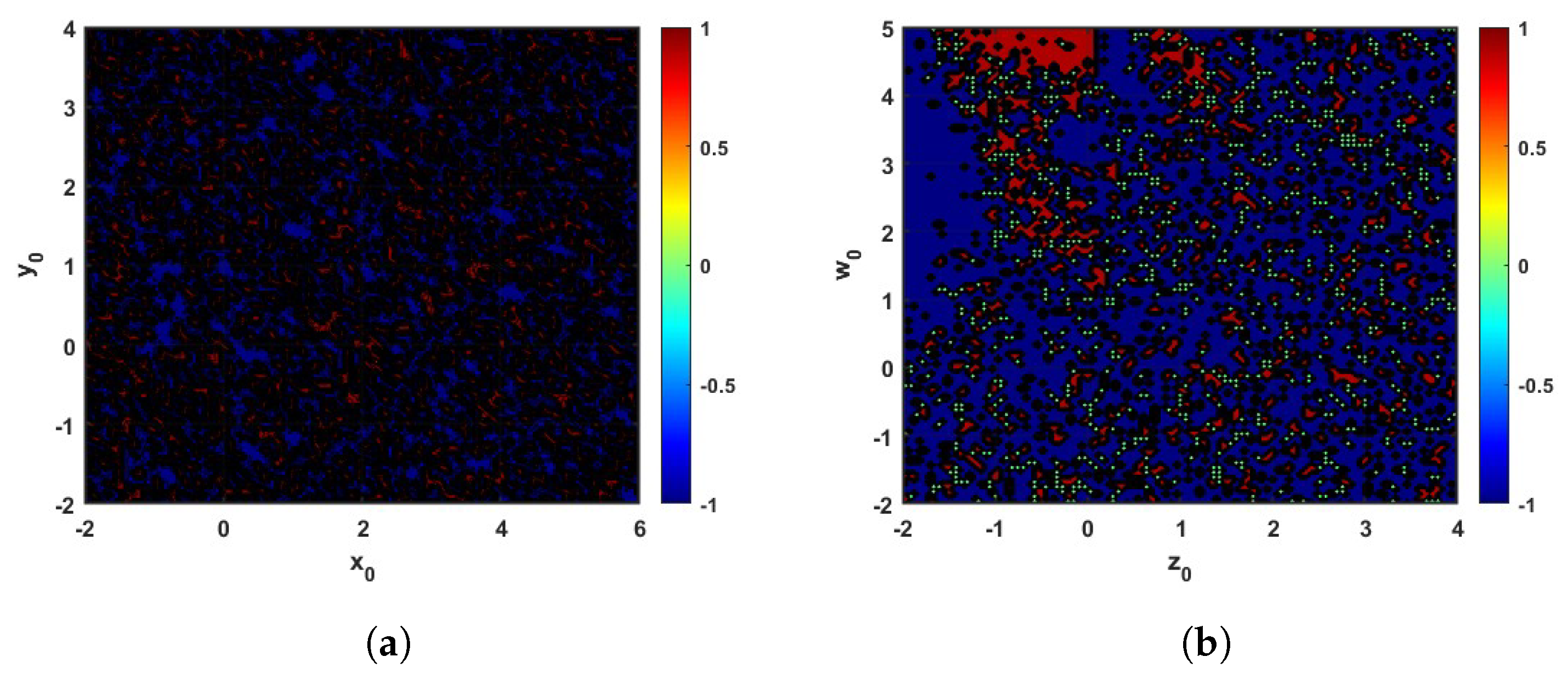
2.1. Stability Analysis

In what follows, we examine the key characteristics of complex dynamic systems, including stability, dissipativity, Lyapunov exponents (LEs), and the bifurcation diagram. To find the stability, the following algebraic equations need to be solved:

$$\alpha y(z-w)=0,$$

(2)

$$x\left|x\right|-y\left|y\right|-w\left|w\right|=0,$$

(3)

$$sign\left(yw\right)-\beta xy=0,$$

(4)

$$x-w=0.$$

(5)

One can obtain the equilibrium points of the proposed dynamic system by substituting Equation (5) into (3), which yields the following three cases:

I.

The origin $E_1=(0,0,0,0)$ is the equilibrium point for the proposed oscillator.

II.

When $x=y=w=0$ and $z\ne 0,$ a line of equilibria appears as $E_2=(0,0,z,0).$

III.

When $y=0,$ $z\ne 0$, and $x=w\ne 0,$ we have spherical equilibria $E_3=(x,0,z,w)$, where $x^2+z^2+w^2=1.$

Accordingly, to check the stability of the given equilibrium points $E_p(x_p,y_p,z_p,w_p)$, $(p=1,2,3),$ first, we present the Jacobian matrix of the proposed oscillator (1) as follows:

$$J=\left[\begin{array}{cccc}0& \alpha (z-w)& \alpha y& -\alpha y\\ \\ {\displaystyle \frac{2x^2}{\left|x\right|}}& {\displaystyle \frac{2y^2}{\left|y\right|}}& 0& {\displaystyle \frac{2w^2}{\left|w\right|}}\\ -\alpha y& 2w\delta \left(yw\right)-\alpha x& 0& 2y\delta \left(yw\right)\\ \\ 1& 0& 0& -1\end{array}\right],$$

(6)

where $\delta \left(x\right)$ is the Dirac function.

Thus, when $\alpha =1.45$ and $\beta =2.95$, the eigenvalues of the corresponding $\mathbf{J}\left(E_p\right)$$(p=1,2,3)$ can not be calculated according to the values of $x=0, y=0, w=0$, which means that the entries in the second row ($a_{2,1}={\displaystyle \frac{2x^2}{\left|x\right|}}, a_{2,2}={\displaystyle \frac{2y^2}{\left|y\right|}}$, and $a_{2,4}={\displaystyle \frac{2w^2}{\left|w\right|}}$) of $\mathbf{J}$ are undefined. Therefore, the stability of oscillator (1) can not be determined by the direct Lyapunov method. Analytically, to find the stability, we apply the L’Hopital rule: if ${\displaystyle \frac{f\left(x\right)}{g\left(x\right)}}$, where $f\left(x\right)$ and $g\left(x\right)$ are continuous functions, then ${lim}_{x\to r}{\displaystyle \frac{f\left(x\right)}{g\left(x\right)}}={lim}_{x\to r}{\displaystyle \frac{f^{\prime }\left(x\right)}{g^{\prime }\left(x\right)}}.$ Let us apply the L’Hopital rule for $a_{1,2}, a_{2,2}, a_{2,4}.$ For instance, $a_{2,1}={\displaystyle \frac{-2x^2}{\left|x\right|}}$, where $f\left(x\right)=-2x^2$ and $g\left(x\right)=\left|x\right|.$ Thus,

$$f^{\prime }\left(x\right)={\displaystyle \frac{d}{dx}}(-2x^2)=-4x$$

and

$$g^{\prime }\left(x\right)={\displaystyle \frac{d}{dx}}\left|x\right|=\left\{\begin{array}{cc}1,\mathrm{if}x>0;\hfill & \\ -1,\mathrm{if}x<0.\hfill \end{array}\right.$$

By applying the L’Hopital rule, we have

$$\underset{x\to 0}{lim}{\displaystyle \frac{-2x^2}{\left|x\right|}}=\underset{x\to 0}{lim}{\displaystyle \frac{-4x}{\pm 1}}=\underset{x\to 0}{lim}\left\{\begin{array}{cc}-4x,\mathrm{if}x>0;\hfill & \\ 4x,\mathrm{if}x<0.\hfill \end{array}\right.=0.$$

This confirms that ${lim}_{x\to 0}{\displaystyle \frac{-2x^2}{\left|x\right|}}=0.$ This way, we can now easily say that the eigenvalues of the Jacobin matrix $\mathbf{J}$ at $E_{1,2}$ are ${\lambda }_1=-1$ and ${\lambda }_{2,3}=0$, which are stable equilibrium points.

2.2. Complexity of Oscillator (1)

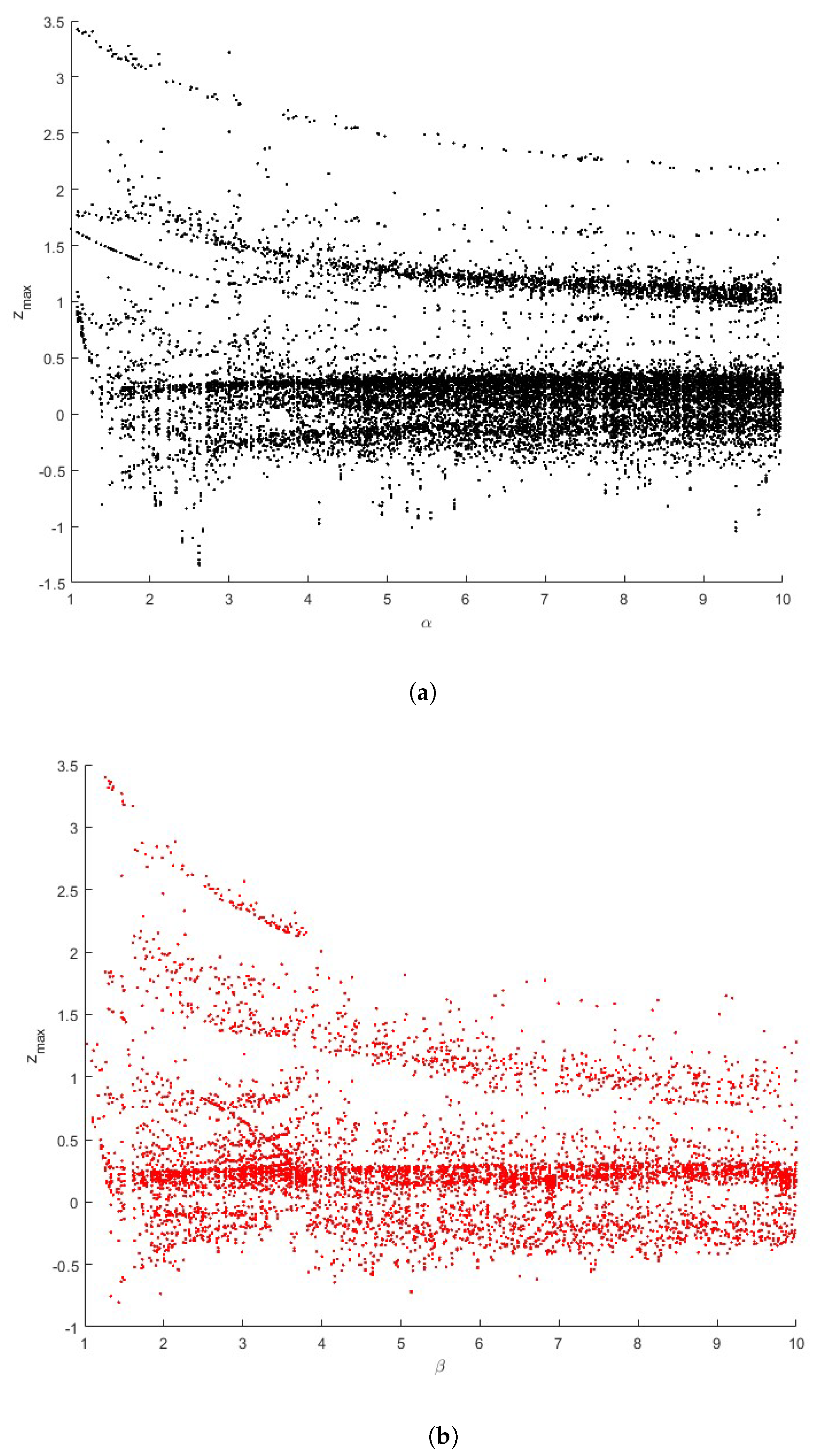
Firstly, the dissipative property of the proposed system (1) is tested:

$$V={\displaystyle \frac{\partial \dot{x}}{\partial x}}+{\displaystyle \frac{\partial \dot{y}}{\partial y}}+{\displaystyle \frac{\partial \dot{z}}{\partial z}}+{\displaystyle \frac{\partial \dot{w}}{\partial w}}=-{\displaystyle \frac{2y^2}{\left|y\right|}}-1.$$

(7)

From (7), the disspativity of the trajectory of oscillator (1) is not clear, since it was calculated using the value of $-2\ast y^2\left(t\right)/\left|y\left(t\right)\right|-1$ as $t\to \infty .$ In [29], the authors established the average value of any function of time $q\left(t\right)$ by

$$\overline{q}\left(t\right)=\underset{t\to \infty }{lim}({\int }_{t_0}^{t}q\left(t\right)dt/t-t_0).$$

(8)

By using Formula (8), it is easy to find that the average value of $-2y^2\left(t\right)/\left|y\left(t\right)\right|-1<0$ and system (1) is dissipative. Numerically, Figure 1 shows that the average value of $-2y^2\left(t\right)/\left|y\left(t\right)\right|-1=-2.08$ for $t=1000.$ Thus, the system orbit shrinks into a subset with zero volume, and the asymmetric motion folds to coin chaotic attractors, which is verified by the numerical simulations in the next section.

Secondly, for $\alpha =1.45, \beta =2.95$ and IC $x_0=1, y_0=0.5, z_0=1, w_0=0.5,$ the proposed system exhibits hyperchaotic behavior, where the phases are shown in Figure 2a–d and the projection of $x, y, z, w$ is shwon in Figure 3. The Lyapunov exponents (LEs) of system (1) are $L_1=0.487420, L_2=0.331870, L_3=0,$ $L_4=-1.561768;$ see Figure 4a. Due to the LEs, the Kaplan–Yorke fractional dimension $D_{KY}=3.524591$. Therefore, it indicates a strange attractor. Figure 4b shows that the attractor of oscillator 1 touches equilibria $E_3$ for radii of less than 6. In addition, to fully demonstrate the dynamic behavior of the introduced system, we provide the simulation results of the maximum of the two positive Lyapunov exponents, which vary with parameters $\alpha \in [1,2]$ and $\beta \in [2,3]$, as shown in Figure 4e,f, which determine hyperchaotic motion within a large range.

3. Bifurcation

To display the system’s dynamics over a broad range of its two parameters $\alpha$ and $\beta$, in Figure 5a, we plot the bifurcation diagram for $\alpha \in [1,10]$ with $\beta =2.95$. Additionally, in Figure 5b, we plot the bifurcation diagram for $\beta \in [1,10]$ with $\alpha =1.45.$ The initial conditions of the proposed system are $x_0=1,y_0=0.5,z_0=1,$ and $w_0=0.5$.

In addition, attraction basins provide an additional tool for examining the behavior of the corresponding dynamic systems. Figure 6 shows the attraction basins for the dynamics of System (1) with $\alpha =1.45,\beta =2.95.$ In particular, we set two of the initial conditions to zero and change the others. The attraction basins are plotted in Figure 6a for the $x_0-y_0$ plane with $x_0\in [-2,6]$ and $y_0\in [-2,4]$ and in Figure 6b $z_0-w_0$ plane with $z_0\in [-2,4], w_0\in [-2,5]$. The intervals of initial conditions were chosen to avoid the torus attractors. Black and red represent chaotic and periodic solutions, respectively. For periodic solutions, the representing color encodes the period.

4. Poincaré Cross-Section

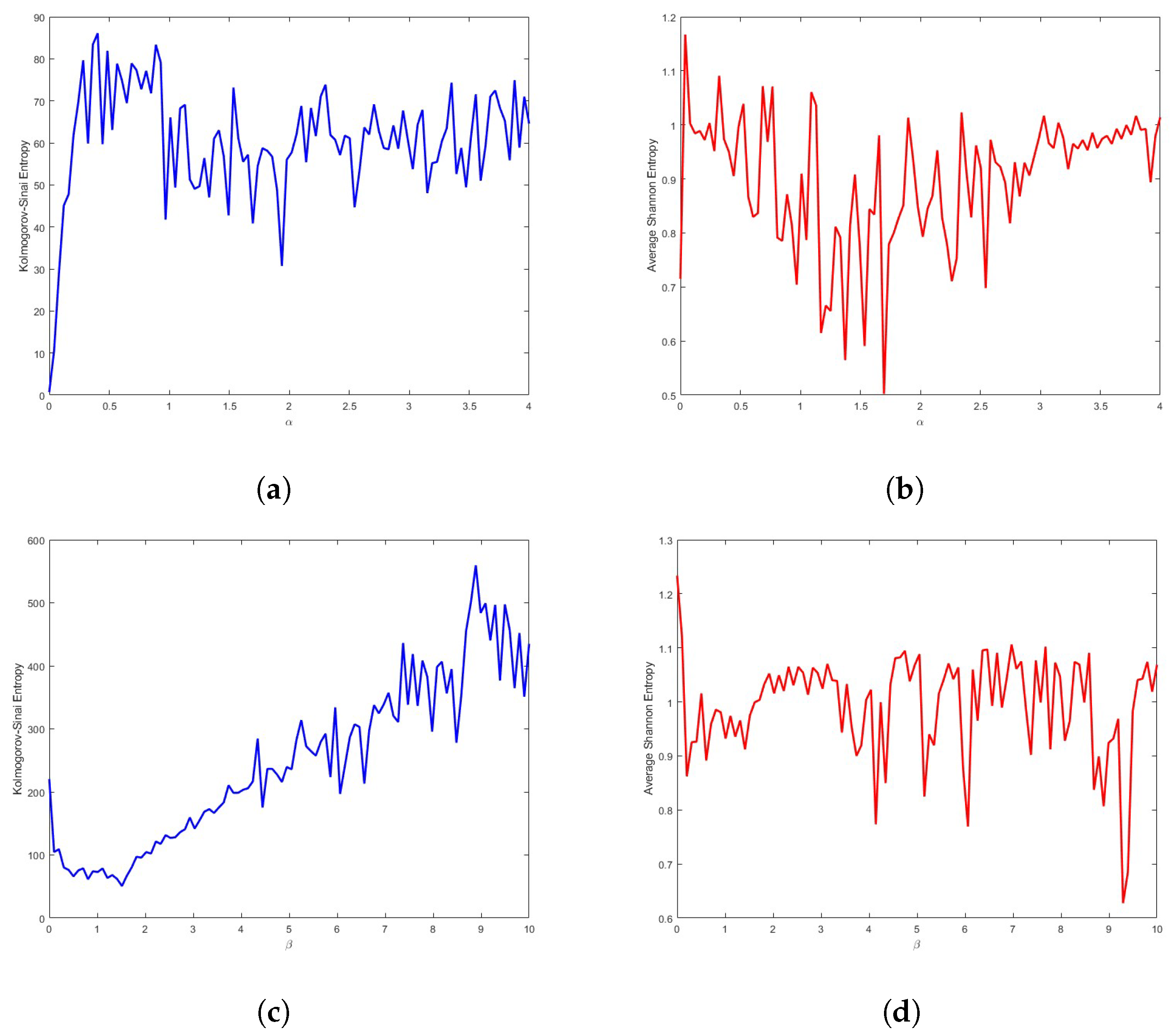
A crucial tool for examining a chaotic system’s folding characteristics and bifurcation is the Poincaré approach. For the 4D hyperchaos system under consideration, we take the following:

$$\begin{array}{cc}\hfill \tilde{\mathrm{\Sigma }}1& ={\left[\begin{array}{cccc}x& y& z& w\end{array}\right]}^T\in {\mathbb{R}}^3\mid x=1,\hfill \\ \hfill \tilde{\mathrm{\Sigma }}2& ={\left[\begin{array}{cccc}x& y& z& w\end{array}\right]}^T\in {\mathbb{R}}^3\mid y=1,\hfill \\ \hfill \tilde{\mathrm{\Sigma }}3& ={\left[\begin{array}{cccc}x& y& z& w\end{array}\right]}^T\in {\mathbb{R}}^3\mid z=1,\hfill \\ \hfill \tilde{\mathrm{\Sigma }}4& ={\left[\begin{array}{cccc}x& y& z& w\end{array}\right]}^T\in {\mathbb{R}}^3\mid w=1.\hfill \end{array}$$

First, let us fix the parameters $\alpha =1.45$ and $\beta =2.95.$ We investigated the Poincaré map projection for $(x,y)$ and $(z,w).$ Figure 4c,d represent the Poincaré cross-section on the $z-w$ plane when $x=y=0$ and on the $x-y$ plane when $z=w=0$ after the steady state is reached (i.e., $t>100).$ As can be seen from Figure 4c,d, the Poincaré map has multiple limbs with discrete bifurcations in multiple directions, providing diverse dynamics for System (3). We see that the Poincaré map’s branches are joined to form a single attractor.

5. Entropy

System complexity over time is one of the most interesting questions in dynamic systems theory. In 19th century, the thermodynamic concept of “entropy” provided an important tool for measuring the complexity of such systems. Nowadays, entropy is a fundamental concept in information theory and in the analysis of chemical reaction, among others.

For each possible state $i,$ ${\sigma }_i$ is probability i; then, the Shannon entropy is defined by

$$Ent=-\sum _i{\sigma }_{i}log\left({\sigma }_i\right).$$

(9)

Additionally, let $\mathrm{\Omega }$ denote the state space, let ${\xi }_i$ be the first Poincaré recurrence time, and let $\rho$ be the D-dimensional box in $\mathrm{\Omega }$ with side $\epsilon$, where $x_i$ is observed. Now, $\gamma (\xi ,\rho )$ denotes the probability distribution of ${\xi }_i$. In what follows, the well-known Kolmogorov–Sinai entropy is defined as

$$H_{KSE}\left(\rho \left[\epsilon \right]\right)={\displaystyle \frac{1}{{\xi }_{min}\rho \left[\epsilon \right]}}\sum _{\xi }\gamma (\xi ,\rho \left[\epsilon \right])log\left({\displaystyle \frac{1}{\gamma (\xi ,\rho [\epsilon \left]\right)}}\right)$$

(10)

The entropy in Equation (10) is applicable and highly positive for chaotic dynamics. Additionally, approaching the bifurcation points can be detected in the entropy if the transient time is not subtracted. This is because the state becomes distributed at bifurcation points due to slowness.

Particularly, Figure 7a,c show the Shannon and Kolmogorov–Sinai entropies for $\alpha \in [0,4],$ respectively. Figure 7b,d show the Shannon and Kolmogorov–Sinai entropies for $\beta \in [0,10],$ respectively.

Figure 7 shows that by increasing parameters $\alpha$ and $\beta$, Kolmogorov–Sinai entropy has increasingly positive values in hyperchaos regions, while the Shannon entropy is not highly increased. This means that the complexity of the proposed oscillator is high in chaos regions.

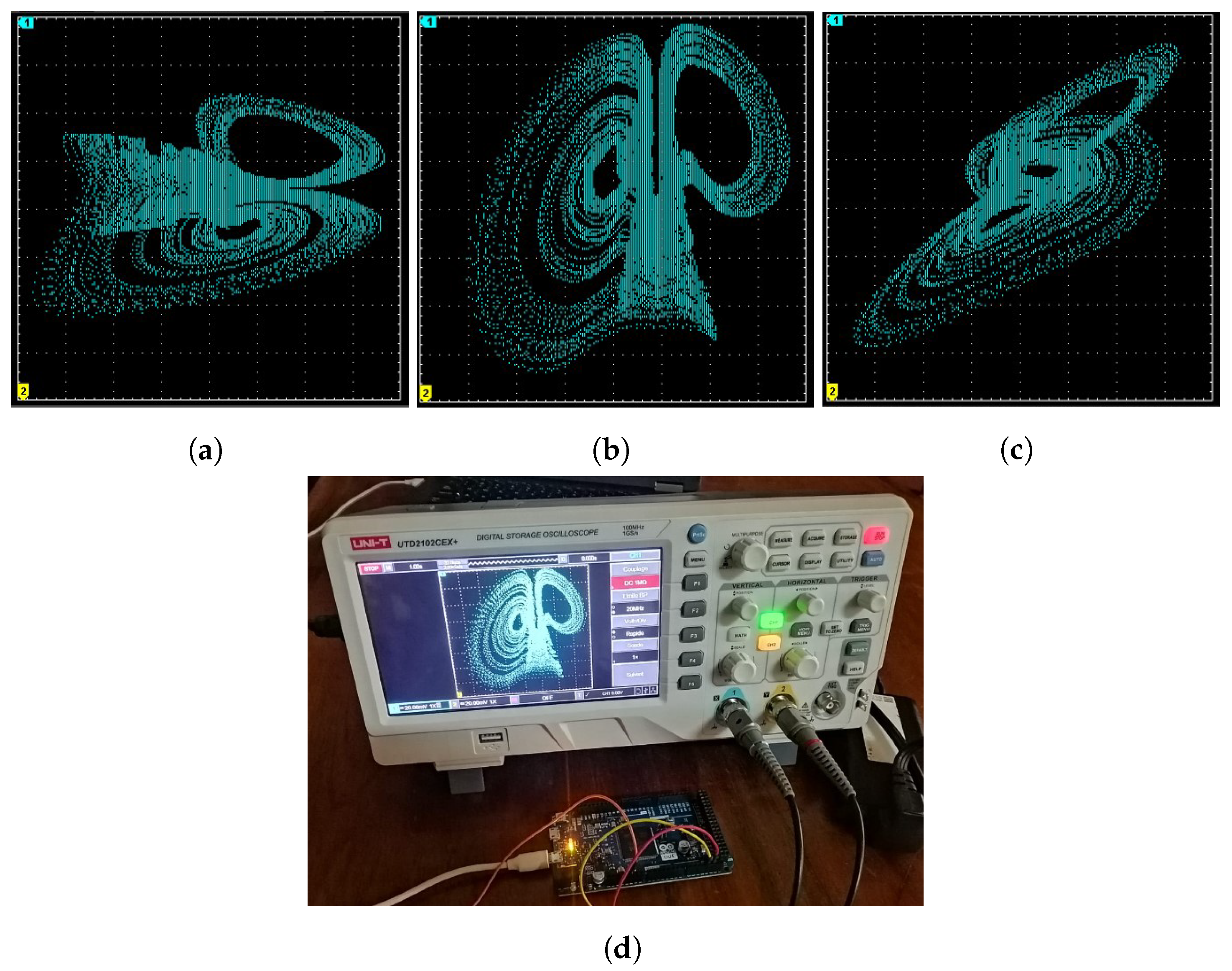
6. Microcontroller Implementation of 4D Oscillator

After a numerical study of a hyperchaotic system, an experimental study is required to validate the numerical results. This experimental study is generally carried out in one of two ways. The first consists of using electronic components to build integrator circuits for integrating the various equations that constitute the chaotic system in question. The second, which is the most widely used today, is based on the use of digital processing boards such as the Arduino board, the DSP board, the FPGA board, or one of many others. A digital processing board makes it possible to combine the performance of programming with that of electronics. More specifically, it enables the programming of electronic systems. The main advantage of programmed electronics is that they greatly simplify electronic circuits and consequently reduce not only the cost of production but also the workload involved in designing an electronic board. It should be noted that each board is equipped with a microcontroller with specific characteristics. The choice of board depends very much on the complexity of the chaotic system being implemented. Compared to electronic circuit implementation, microcontroller implementation provides numerous benefits, including quick computation time, excellent stability and accuracy, and high flexibility, and changing the system’s initial conditions and settings is simple. Due to these factors, we implemented the four-dimensional hyperchaotic oscillator by using a microcontroller called “Arduino Due”. One benefit of this card is that it features an embedded digital-to-analog converter, making installation easier. Using a Voltcraft D50-1062D, which is a dual-channel digital oscilloscope, the experimental observations were obtained. We discretized the proposed hyperchaotic oscillator with the fourth-order Runge–Kutta method, where the step size of the discretization was equal to 0.001. The results for $\alpha =1.45$, $\beta =2.95$, and $x_0=1,y_0=0.5,z_0=1,w_0=0.5$ are shown in Figure 8a–c. Figure 8d shows the related practical diagrams of the phases. It is obvious that the experimental and numerical results coincide. This demonstrates that the Arduino Due microcontroller could successfully simulate the proposed oscillator’s dynamics.

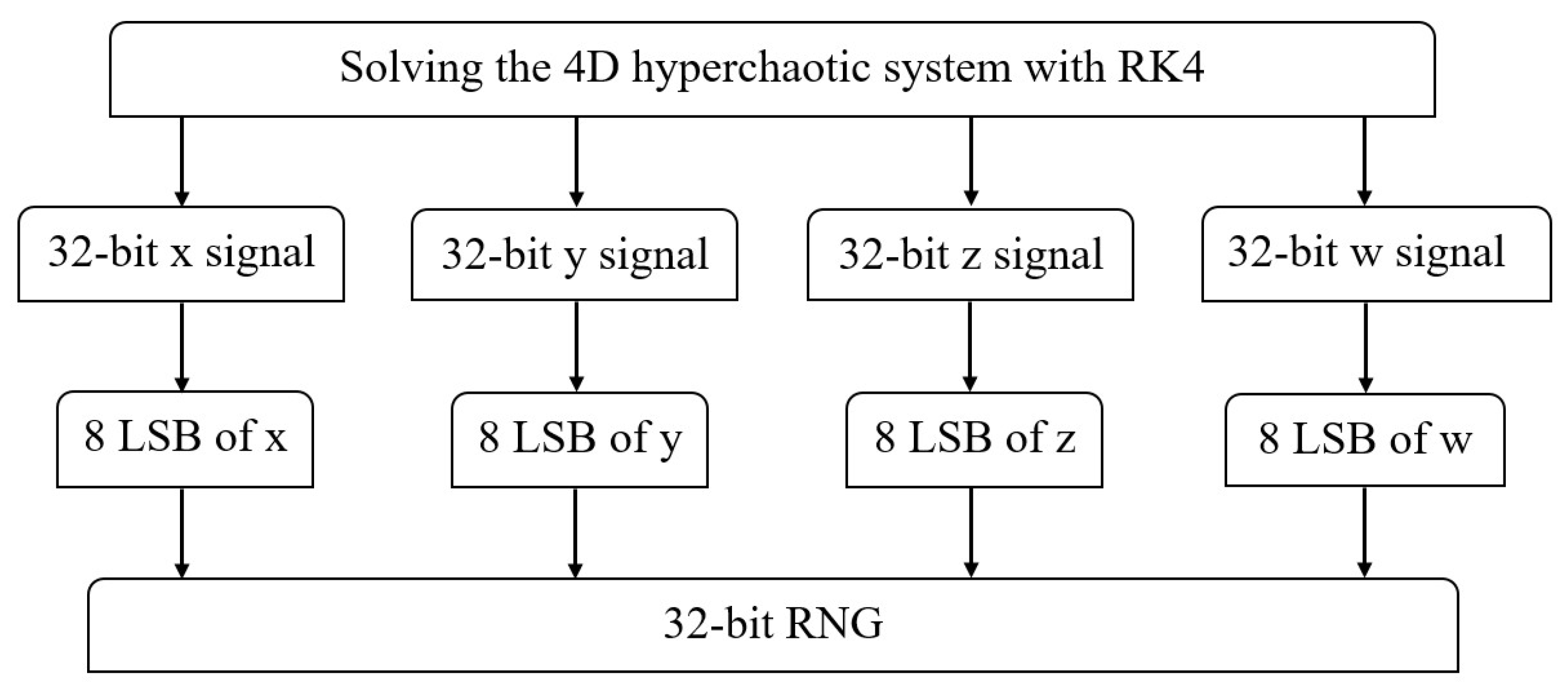
7. Implementation for RNG

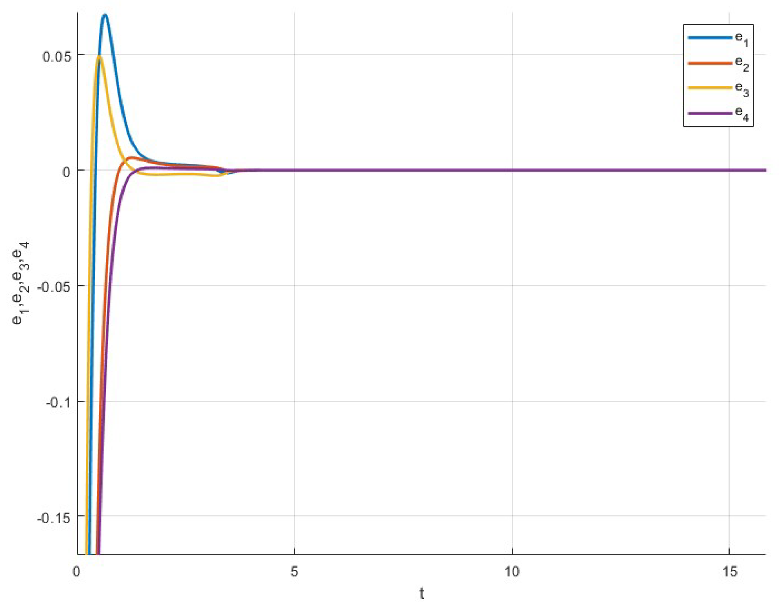
Applications such as text, audio, and image encryption using hyperchaotic systems require the hyperchaotic signals generated by such systems to be highly random to increase the security level of data transmission. To achieve this, the hyperchaotic signals from the system under study were used to design a random bit generator. The generated bits were then tested (using the NIST test) to ensure that they were effectively random. The NIST test is a set of 16 subtests, all of which must be validated simultaneously. If only 1 of the 16 subtests is failed, the test must be repeated until it is passed. At the end of this test, we confirmed that all the state variables $(x,y,z,w)$ of the hyperchaotic system were definitely random. Figure 9 presents the main steps describing the RNG design process.

The process started with the numerical integration of the system. Next, we selected 8 LSBs of each delivered hyperchaotic signal and combined them to form a 32-bit RNG. Finally, such bits were subjected to the NIST test, whose results are recorded in

Table 2. Test results for the $x,y,z,w$ output hyperchaotic signals.

Test Name	p-Value (x)	p-Value (y)	p-Value (z)	p-Value (w)	Results
Frequency	0.25345	0.70692	0.85872	0.92034	demonstrated
Block frequency	0.44118	0.93263	0.19375	0.28412	demonstrated
Runs	0.41489	0.55394	0.90287	0.07540	demonstrated
Longest run of ones	0.97984	0.97531	0.11504	0.21060	demonstrated
Rank	0.74427	0.47236	0.76575	0.46079	demonstrated
DFT	0.50292	0.06783	0.37834	0.77604	demonstrated
No overlapping templates	0.30195	0.05616	0.02864	0.10238	demonstrated
Overlapping templates	0.78749	0.77395	0.90626	0.81761	demonstrated
Universal	0.97158	0.15981	0.46365	0.62048	demonstrated
Linear complexity	0.18993	0.23150	0.92968	0.06544	demonstrated
Serial test 1	0.38527	0.67854	0.17562	0.72572	demonstrated
Serial test 2	0.48301	0.71068	0.53014	0.64265	demonstrated
Approximate entropy	0.14177	0.61022	0.37092	0.94487	demonstrated
Cumulative sums (forward)	0.30197	0.86374	0.51721	0.64392	demonstrated
Random excursions x = 2	0.50579	0.57193	0.99671	0.41986	demonstrated
Random excursion variant x = 8	0.72471	0.03628	0.59473	0.91573	demonstrated

. From the data recorded in Table 2, we can see that all NIST tests were validated, since all p-values of the RNG were superior to 0.001. Therefore, the obtained RNG can be exploited for engineering applications [30] as mentioned above.

8. System Control

In this section, we apply adaptive control, which is a modern method in the control field that has been modified specifically for dynamic systems. Adaptive control mechanisms offer unmatched versatility and efficacy, enabling the smooth adaptation and optimization of control procedures in reaction to variations in system dynamics. This adaptive capacity is especially useful for chaotic systems’ intrinsic unpredictability and complexity. $D,R,Es$, and $CL$ are the driver, response, error estimate, and closed-loop system, respectively.

Next, let us establish the D system as

$$\left\{\begin{array}{c}\dot{u}=\alpha v(q-r)\hfill \\ \dot{v}=u\left|u\right|-v\left|v\right|-r\left|r\right|\hfill \\ \dot{q}=sgn\left(vr\right)-\beta uv\hfill \\ \dot{r}=u-r\hfill \end{array}\right.$$

(11)

Note that the parameters of system D are not valued. S, which represents the adaptive synchronization of an identical D, is given by

$$\left\{\begin{array}{c}\dot{u}=\alpha v(q-r)+{\xi }_1\hfill \\ \dot{v}=u\left|u\right|-v\left|v\right|-r\left|r\right|+{\xi }_2\hfill \\ \dot{q}=sgn\left(vr\right)-\beta uv+{\xi }_3\hfill \\ \dot{r}=u-r+{\xi }_4\hfill \end{array}\right.$$

(12)

where the states are represented by $u,v,q,r$; the not-valued parameters are given as $\alpha ,\beta$; and

$$\mathrm{\Xi }={[{\xi }_1,{\xi }_2,{\xi }_3,{\xi }_4]}^T$$

is the adaptive controller that needs to be identified.

Assume the following:

$$\left\{\begin{array}{c}{\xi }_1=-E_{\alpha }v(q-r)-{\tau }_{1}u\hfill \\ {\xi }_2=-u\left|u\right|+v\left|v\right|+r\left|r\right|-{\tau }_{2}v\hfill \\ {\xi }_3=-sgn\left(vr\right)+E_{\beta }uv-{\tau }_{3}q\hfill \\ {\xi }_4=-u+r-{\tau }_{4}r\hfill \end{array}\right.$$

(13)

where $E_{\alpha }$ and $E_{\beta }$ denote the error estimated parameters, and ${\tau }_1$,${\tau }_2$,${\tau }_3$,${\tau }_4>0$.

Substituting (13) into (12), the $CL$ system is

$$\left\{\begin{array}{c}\dot{u}=-[\alpha -E_{\alpha }]v(q-r)-{\tau }_{1}u\hfill \\ \dot{v}=-{\tau }_{2}v\hfill \\ \dot{q}=-[\beta -E_{\beta }]uv-{\tau }_{3}q\hfill \\ \dot{r}=-{\tau }_{4}r\hfill \end{array}\right.$$

(14)

To simplify, we use the following notation:

$$\left\{\begin{array}{c}{E}_1\left(t\right)=[\alpha -E_{\alpha }];\hfill \\ E_2\left(t\right)=[\beta -E_{\beta }].\end{array}\right.$$

(15)

Due to (15), the derivatives of $E_1\left(t\right)$ and $E_2\left(t\right)$ are given by

$$\left\{\begin{array}{cc}\dot{E_1}=-\dot{E_{\alpha }},\hfill & \\ \dot{E_2}=-\dot{E_{\beta }}.\hfill \end{array}\right.$$

(16)

System (14) is reduced as follows:

$$\left\{\begin{array}{c}\dot{u}=E_{1}v(q-r)-{\tau }_{1}u\hfill \\ \dot{v}=-{\tau }_{2}v\hfill \\ \dot{q}=E_{2}uv-{\tau }_{3}q\hfill \\ \dot{r}=-{\tau }_{4}r\hfill \end{array}\right.$$

(17)

Theorem 1.

If the controllers are chosen as (14) and the parameter’s update laws are as follows:

$$\left\{\begin{array}{cc}\dot{E_1}\left(t\right)=uv(q-r)-\eta (\alpha -E_{\alpha });\hfill & \\ \dot{E_2}\left(t\right)=quv-\eta (\beta -E_{\beta }).\hfill \end{array}\right.$$

(18)

then the synchronization between D and S issatisfied if ${\tau }_1,{\tau }_2,{\tau }_3,{\tau }_4$ are greater than zero.

Proof. 

By using the so-called Lyapunov function

$$V(u,v,q,r,E_1,E_2)={\displaystyle \frac{1}{2}}\left(u^2+v^2+q^2+r^2+E_1^2+E_2^2\right)$$

and differentiating the function V, we have

$$\begin{gathered} \dot{V}(u,v,q,r,E_1,E_2)= \\ =\left(u\dot{u}+v\dot{v}+q\dot{q}+r\dot{r}+E_1\dot{E_1}+E_2\dot{E_2}\right) \end{gathered}$$

Considering the time derivative of the above function along the trajectories of (18), we have

$$\dot{V}=-({\tau }_1{u}^2+{\tau }_2{v}^2+{\tau }_3{q}^2+{\tau }_4{r}^2+\eta E_1^2+\eta E_2^2).$$

(19)

where the function (19) has a negative value when ${\tau }_1,{\tau }_2,{\tau }_3,{\tau }_4$ have a positive value. Furthermore, from the Lyapunov stability, we find that $E_1\left(t\right)\to 0$ and $E_2\left(t\right)\to 0$ are exponentially decreasing for $t\to \infty$. □

Numerical Simulation

We simulated the adaptive control between D and R when the parameter update law (18) is satisfied. Firstly, we set $\alpha =1.45$ and $\beta =2.95$ in system (11). Note that the fourth-order Runge–Kutta method was used for this purpose. Secondly, we set ${\tau }^{\prime }$ and ${\eta }^{\prime }$ as ${\tau }_i={\eta }_j=2,(i=1,\dots ,4;j=1,2).$ The initial values $(0,0,0,0)$ were the estimated parameters, and the initial values of system (11) were established as (1, 1, 1, 1). Where the adaptive control law (18) and the parameter update law were used, equilibrium E = (0, 0, 0, 0) was the limit point of the controlled system, as shown in Figure 10.

9. Conclusions

A 4D hyperchaotic oscillator with a special algebraic property, having spherical and line equilibria, was introduced. Additionally, the bifurcation diagram, Lyapunov exponents, and Poincaré cross-section were tested for the introduced oscillator. The complexity was measured by calculating different kinds of entropies. Moreover, RNG showed the successful application of the proposed oscillator. In addition, we provided the adaptive control for the oscillator. Further exploration of the other dynamics of this introduced system is a potential avenue for future research.

References

1. Cicek, S.; Kocamaz, U.; Uyaroglu, Y. Secure communication with a chaotic system owning. Aeu Int. J. Electron. Commun. 2018, 88, 52–62. [Google Scholar] [CrossRef]
2. Tamba, V.K.; Pham, V.; Shukur, A.A.; Grassi, G.; Momani, S. Oscillator without equilibrium and linear terms: Dynamics and application. Alex. Eng. J. 2024, 97, 376–384. [Google Scholar] [CrossRef]
3. Lin, H.; Wang, C.; Yao, W.; Tan, Y. Chaotic dynamics in a neural network with different types of external stimuli. Commun. Nonlinear Sci. Numer. Simulat. 2020, 90, 105390. [Google Scholar] [CrossRef]
4. Tan, Z.; Hepburn, B.S.; Tucker, C.; Ali, M.K. Pattern recognition using chaotic neural networks. Discret. Dyn. Nat. Soc. 1998, 2, 243–247. [Google Scholar]
5. Wu, L.; Wang, D.; Zhang, C.; Mohammadzadeh, A. Chaotic Synchronization in Mobile Robots. Mathematics 2022, 10, 4568. [Google Scholar] [CrossRef]
6. Korolj, A.; Wu, H.T.; Radisic, M. A healthy dose of chaos: Using fractal frameworks for engineering higher-fidelity biomedical systems. Biomaterials 2019, 219, 119363. [Google Scholar] [CrossRef] [PubMed]
7. Lorenz, E.N. Deterministic Nonperiodic Flow. J. Atmos. Sci. 1963, 20, 130–141. [Google Scholar] [CrossRef]
8. Jafari, S.; Sprott, J.; Golpayegani, S.M.R.H. Elementary quadratic chaotic flows with no equilibria. Phys. Lett. A 2013, 377, 699–702. [Google Scholar] [CrossRef]
9. Wei, Z. Dynamical behaviors of a chaotic system with no equilibria. Phys. Lett. A 2011, 376, 102–108. [Google Scholar] [CrossRef]
10. Lao, S.K.; Shekofteh, Y.; Jafari, S.; Sprott, J. Cost function based on Gaussian mixture model for parameter estimation of a chaotic circuit with a hidden attractor. Int. J. Bifurc. Chaos 2014, 24, 1450010. [Google Scholar] [CrossRef]
11. Wang, X.; Chen, G. A chaotic system with only one stable equilibrium. Commun. Nonlinear Sci. Numer. Simul. 2012, 17, 1264–1272. [Google Scholar] [CrossRef]
12. Kapitaniak, T.; Mohammadi, S.A.; Mekhilef, S.; Alsaadi, F.E.; Hayat, T.; Pham, V.T. A New Chaotic System with Stable Equilibrium: Entropy Analysis, Parameter Estimation, and Circuit Design. Entropy 2018, 20, 670. [Google Scholar] [CrossRef] [PubMed]
13. Jafari, S.; Sprott, J. Simple chaotic flows with a line equilibrium. Chaos Solitons Fractals 2013, 57, 79–84. [Google Scholar] [CrossRef]
14. Rajagopal, K.; Karthikeyan, A.; Srinivasan, A. Bifurcation and chaos in time delayed fractional order chaotic oscillator and its sliding mode synchronization with uncertainties. Chaos Solitons Fractals 2017, 103, 347–356. [Google Scholar] [CrossRef]
15. Barati, K.; Jafari, S.; Sprott, J.C.; Pham, V.T. Simple Chaotic Flows with a Curve of Equilibria. Int. J. Bifurc. Chaos 2016, 26, 1630034. [Google Scholar] [CrossRef]
16. Tolba, M.F.; Said, L.A.; Madian, A.H.; Radwan, A.G. FPGA implementation of fractional-order integrator and differentiator based on Grunwald Letnikov’s definition. In Proceedings of the 29th International Conference on Microelectronics (ICM), Beirut, Lebanon, 10–13 December 2017; pp. 1–4. [Google Scholar]
17. Ismail, S.M.; Said, L.A.; Rezk, A.A.; Radwan, A.G.; Madian, A.H.; Abu-Elyazeed, M.F.; Soliman, A.M. Generalized fractional logistic map encryption system based on FPGA. EU-Int. J. Electron. Commun. 2017, 80, 114–126. [Google Scholar] [CrossRef]
18. Leonov, G.; Kuznetsov, N.; Mokaev, T. Hidden attractor and homoclinic orbit in Lorenz-like system describing convective fluid motion in rotating cavity. Commun. Nonlinear Sci. Numer. Simul. 2015, 28, 166–174. [Google Scholar] [CrossRef]
19. Rossler, O. An equation for hyperchaos. Phys. Lett. A 1979, 71, 155–157. [Google Scholar] [CrossRef]
20. Barboza, R. Dynamics of a hyperchoatic Lorenz system. Int. J. Bifurc. Chaos 2007, 17, 4285–4290. [Google Scholar] [CrossRef]
21. Neimark, Y.; Shilnikov, L. A condition for the generation of periodic motions. Sov. Math. Docklady 1963, 163, 1261–1264. [Google Scholar]
22. Benkouider, K.; Vaidyanathan, S.; Sambas, A.; Cuautle, E.; Abd EL-latif, A.; Abd-EL-Atty, B.; Bermudez-Marquez, C.; Sulaman, I.; Awwal, A.; Kuman, P. A New 5-D Multistable Hyperchaotic System With Three Positive Lyapunov Exponents: Bifurcation Analysis, Circuit Design, FPGA Realization and Image Encryption. IEEE Access 2022, 10, 90111–90132. [Google Scholar] [CrossRef]
23. Peng, Z.; Yu, W.; Wang, J.; Zhou, Z.; Chen, J.; Zhong, G. Secure communication based on microcontroller unit with a novel five-dimensional hyperchaotic system. Arabian J. Sci. Eng. 2021, 47, 813–828. [Google Scholar] [CrossRef]
24. Vaidyanathan, S. A Novel 5-D Hyperchaotic System with a Line of Equilibrium Points and Its Adaptive Control. Advances and Applications in Chaotic Systems. Stud. Comput. Intell. 2016, 636, 471–494. [Google Scholar]
25. Chunbiao, L.; Sprott, J.C.; Wesley, T. Bistability in a Hyperchaotic System with a Line Equilibrium. J. Exp. Theor. Phys. 2014, 118, 494–500. [Google Scholar]
26. Singh, J.; Roy, B.K. The simplest 4-D chaotic system with line of equilibria, chaotic 2-torus and 3-torus behaviour. Nonlinear Dyn. 2017, 89, 1845–1862. [Google Scholar] [CrossRef]
27. Singh, J.; Jafari, K.R.S. New family of 4-D hyperchaotic and chaotic systems with quadric surfaces of equilibria. Chaos Solitons Fractals 2018, 106, 243–257. [Google Scholar] [CrossRef]
28. Yuming, C.; Qigui, Y. A new Lorenz-type hyperchaotic system with a curve of equilibria. Math. Comput. Simul. 2015, 112, 40–55. [Google Scholar]
29. Wang, Z.; Xu, Z.; Mliki, E.; Agkgu, A.; Pham, V.-T.; Jafari, S. A new chaotic attractor around a pre-located ring. J. Int. Bifurc. Chaos 2017, 27, 1–10. [Google Scholar] [CrossRef]
30. Diffie, W.; Hellman, M.E. Multiuser cryptographic techniques. In Proceedings of the June 7–10, 1976, National Computer Conference and Exposition; ACM: New York, NY, USA, 1976; pp. 109–112. [Google Scholar]
Figure 1. Average value of V.
Symmetry 16 01341 g001
Figure 2. The phases of oscillator (1) when α = 4 , β = 1.5 : (a) ‘xy’, (b) ‘yz’ (c) ‘zw’ (d) 3D projection ‘xyz’.
Symmetry 16 01341 g002
Figure 3. Projection ( x , y , z , w ) of oscillator (1).
Symmetry 16 01341 g003
Figure 4. (a) Lyapunov exponents of oscillator (1). (b) E 3 when the radius is equal to 3 (blue) and 7 (green); (c) Poincaré cross-section when x = y = 0 ; (d) Poincaré cross section when z = w = 0 ; (e,f) the maximum of the two positive Lyapunov exponents with varying α and β , respectively.
Symmetry 16 01341 g004
Figure 5. (a) Bifurcation diagram for 1 α 10 (black). (b) Bifurcation diagram for 1 β 10 (red).
Symmetry 16 01341 g005
Figure 6. Basin of attraction. (a) z 0 = w 0 = 0 with x 0 [−2, 6] and y 0 [−2, 4]; (b) x 0 = y 0 = 0 with z 0 [−2, 4], w 0 [−2, 5]. Black and red represent chaotic and periodic solutions, respectively.
Symmetry 16 01341 g006
Figure 7. (a,c) Shannon and Kolmogorov–Sinai entropies for α [ 0 , 4 ] , respectively; (b,d) Shannon and Kolmogorov–Sinai entropies for β [ 0 , 10 ] , respectively.
Symmetry 16 01341 g007
Figure 8. The practical test of system (1): (a) V x V w , (b) V x V z , and (c) V x V y . (d) Snapshot of the hardware testing platform.
Symmetry 16 01341 g008
Figure 9. Description of the RNG design process.
Symmetry 16 01341 g009
Figure 10. Time series of anti-synchronization for error of dynamic system (18) with controller (14).
Symmetry 16 01341 g010