Parameter Estimation of Uncertain Differential Equations Driven by Threshold Ornstein–Uhlenbeck Process with Application to U.S. Treasury Rate Analysis

Abstract

Uncertain differential equations, as an alternative to stochastic differential equations, have proved to be extremely powerful across various fields, especially in finance theory. The issue of parameter estimation for uncertain differential equations is the key step in mathematical modeling and simulation, which is very difficult, especially when the corresponding terms are driven by some complicated uncertain processes. In this paper, we propose the uncertainty counterpart of the threshold Ornstein–Uhlenbeck process in probability, named the uncertain threshold Ornstein–Uhlenbeck process, filling the gaps of the corresponding research in uncertainty theory. We then explore the parameter estimation problem under different scenarios, including cases where certain parameters are known in advance while others remain unknown. Numerical examples are provided to illustrate our method proposed. We also apply the method to study the term structure of the U.S. Treasury rates over a specific period, which can be modeled by the uncertain threshold Ornstein–Uhlenbeck process mentioned in this paper. The paper concludes with brief remarks and possible future directions.

1. Introduction

1.1. Background and Motivation

Many models related to probabilistic noise and fluctuations in engineering, industry, physics, environment science, and finance are driven by stochastic differential equations (SDEs), which were first proposed by Itô [1] and have now been developed into Itô stochastic calculus (see [2,3,4]). However, some vital deficiencies in the models related to SDEs are mentioned by Liu [5]. In particular, Liu [6] disproved that real stock prices follow some stochastic differential equations by checking numerous examples. To provide a strict and solid foundation for his viewpoint, one theoretical system of mathematics called uncertainty theory was initiated by Liu [5] based on several mathematical axioms.

Uncertain differential equations, introduced by Liu [7] as an alternative to stochastic differential equations, are driven by Liu processes. These equations are designed to describe some complicated mechanisms in the framework of uncertainty theory. Many results on uncertain differential equations have appeared since they were first introduced. For instance, the conditions of the existence and uniqueness of the corresponding solutions were first obtained by Chen and Liu [8]; many different versions of the stability of the solutions were studied in [9,10,11]. To obtain the solution of general uncertain differential equations, many approximate approaches based on numerical methods and algorithms are designed in [12,13,14,15,16].

The threshold Ornstein–Uhlenbeck process, in the framework of classical probability, has been studied extensively and applied to financial markets already (see [17,18,19]). However, as was proved in Liu [6], real stock prices (including interest rates and currency exchange rates) do not follow any stochastic differential equations. For more detailed information on the reason why uncertainty theory is more appropriate than the theory of Itô stochastic calculus, see Appendix B of the monograph [5]. In other words, uncertain versions of stochastic models are necessary to study the phenomena in finance. As for interest rate models, one term structure model of interest rates in the framework of uncertainty theory was first proposed by Chen and Gao [20]; and one uncertain interest rate model for the Shanghai Interbank Offered Rate was presented by Yang and Ke in [21] very recently. The main motivation of this paper is to establish an uncertain counterpart of the threshold Ornstein–Uhlenbeck process to study the U.S. interest rate, filling the gaps of the corresponding research in uncertainty theory.

1.2. Literature Review

Uncertain differential equations have proved to be extremely powerful across various fields, especially in finance. For more theoretical results on uncertain differential equations, refer to the book by Yao [22]. In fact, uncertain finance theory, which is considered as one of the key components of uncertainty theory, can be traced back to the work [6] by Liu. To be specific, the assumption that stock prices follow stochastic differential equations in stochastic finance theory was challenged by showing a convincing paradox why it is impossible for real stock prices to follow any stochastic differential equations in [6]. To support this viewpoint, numerous empirical examples were obtained. For instance, an uncertain stock model and the corresponding American option pricing formulas were shown by Chen [23]; and the currency exchange issues were discussed by Liu et al. [24]. Numerous financial derivatives in uncertain financial markets were actively developed very recently, including shout options [25], knock-out options [26], and carbon swap [27], among others. See

Table 1. Related works on uncertain finance.

Author	Research	Year
Chen [23]	American option pricing	2011
Chen and Gao [20]	Uncertain term structure model	2013
Liu et al. [24]	Uncertain currency model	2015
Liu and Li [27]	Carbon swap	2024
Jia  et al.  [26]	Knock-out option	2024
Yang and Ke [21]	Uncertain interest rate model	2024

for a brief overview of the derivatives in the uncertain financial markets mentioned above.

One of the fundamental issues is how to estimate the unknown terms in an uncertain differential equation to fit the observed data as much as possible. Many methods have been proposed in this direction and we list some of them as follows: the least squares estimation method was derived by Sheng et al. [28]; moment estimation was obtained by Yao and Liu [29], and later was extended to generalized moment estimation by Liu [30]; the maximum likelihood estimation method was investigated by Liu and Liu [31]; the minimum cover estimation method was developed by Yang et al. [32]; and one novel approach based on estimating functions was explored by Li and Xia [33] very recently. Some nonparametric methods were also developed, such as those discussed in [34,35]. See

Table 2. Related works on parameter estimation for UDEs.

Author	Method	Year
Sheng et al. [28]	Least squares	2019
Yao and Liu [29]	Moment method	2020
Yang et al. [32]	Minimum cover estimation	2020
Liu  [30]	Generalized moment method	2021
Liu and Liu [31]	Maximum likelihood estimation	2022
He et al.  [35]	Nonparametric method	2023
Li and Xia  [36]	Nadaraya–Watson method	2023
Li and Xia  [33]	Estimation function method	2024
Wang et al.  [34]	Threshold weighted moment method	2024

for a brief overview of all the methods for UDEs mentioned above.

1.3. Contribution

All in all, uncertain differential equations and related models are studied extensively nowadays, which implies more advanced models need to be explored in order to meet the challenge brought by new scientific issues in an era of big data.

Our main contributions are as follows. First, one novel uncertain model, an uncertain differential equation driven by an uncertain Ornstein–Uhlenbeck process, is introduced in this paper. Second, the parameter estimation issue of the model mentioned in several different cases is discussed. Finally, one empirical study in the financial market is also added to demonstrate the application of our model.

1.4. Organization of the Paper

The organization of the paper is as follows. Some preliminaries about definitions and results of uncertain differential equations are reviewed in Section 2. The threshold uncertain Ornstein–Uhlenbeck process is introduced and the parameter estimation issues are discussed in Section 3. Two numerical examples are performed in Section 4. One empirical study in the financial market based on the uncertain model proposed in this paper is included in Section 5. Finally, Section 6 presents a concise conclusion.

2. Preliminaries

To make this paper more readable, some necessary definitions and results about uncertain differential equations are reviewed briefly at the beginning of this paper. The first key concept in uncertainty theory, named an uncertain measure, is defined as follows.

Definition 1

(Liu [5]). Let $\mathcal{L}$ be a σ-algebra on a nonempty set Γ. A set function $\mathcal{M}:\mathcal{L}\to [0,1]$ is called an uncertain measure if it satisfies the following three axioms:

• Normality axiom: $\mathcal{M}\left(\mathrm{\Gamma }\right)=1$ for the universal set Γ.
• Duality axiom: $\mathcal{M}\left(\mathrm{\Lambda }\right)+\mathcal{M}\left({\mathrm{\Lambda }}^c\right)=1$ for any event $\mathrm{\Lambda }\in \mathcal{L}.$
• Subadditivity axiom: For every countable sequence of events ${\mathrm{\Lambda }}_1,{\mathrm{\Lambda }}_2,\cdots$, we have

  $$\mathcal{M}\left\{\bigcup _{i=1}^{\infty }{\mathrm{\Lambda }}_i\right\}\le \sum _{i=1}^{\infty }\mathcal{M}\left\{{\mathrm{\Lambda }}_i\right\}.$$

The fourth axiom of uncertainty theory in order to consolidate the framework of uncertain theory is proposed by Liu [7] as follows:

• Product axiom: Let $({\mathrm{\Gamma }}_k,{\mathcal{L}}_k,{\mathcal{M}}_k)$ be uncertainty spaces for $k=1,2,\cdots$. Then, the product uncertain measure error is an uncertain measure satisfying

  $$\mathcal{M}\left\{\prod _{k=1}^{\infty }{\mathrm{\Lambda }}_k\right\}=\underset{k=1}{\overset{\infty }{\bigwedge }}{\mathcal{M}}_k\left\{{\mathrm{\Lambda }}_k\right\},$$

  where ${\mathrm{\Lambda }}_k$ are arbitrary chosen events from ${\mathcal{L}}_k$ for $k=1,2,\cdots ,$ respectively.

Definition 2

(Liu [5]). The uncertainty distribution of an uncertain variable ξ is defined by

$$\mathrm{\Phi }\left(x\right)=\mathcal{M}\{\xi \le x\},\forall x\in \mathbb{R}.$$

An uncertain variable $\xi$ is called linear if it has a linear uncertainty distribution

$$\mathrm{\Phi }\left(x\right)=\left\{\begin{array}{cc}0,& \mathrm{if}x<a\hfill \\ {\displaystyle \frac{x-a}{b-a}},& \mathrm{if}a\le x<b\hfill \\ 1,& \mathrm{if}x\ge b.\hfill \end{array}\right.$$

denoted by $\mathcal{L}(a,b)$, where $a,b$ are real numbers with $a<b$.

The linear uncertain variable $\mathcal{L}(0,1)$ has a very basic but important property.

Lemma 1.

Let ξ be some uncertain variable with uncertainty distribution function $\mathrm{\Psi }\left(x\right)$ for $x\in \mathbb{R}$, then

$$\mathrm{\Psi }\left(\xi \right)\sim \mathcal{L}(0,1).$$

i.e., the uncertain variable $\mathrm{\Psi }\left(\xi \right)$ follows the linear uncertainty distribution.

We call $\xi$ normal if its distribution function is

$$\mathrm{\Phi }\left(x\right)={\left(1+exp\left({\displaystyle \frac{\pi (e-x)}{\sqrt{3}\sigma }}\right)\right)}^{-1},x\in \mathbb{R}.$$

We write $\xi \sim \mathcal{N}(e,\sigma )$, where $(e,\sigma )\in (\mathbb{R},{\mathbb{R}}_{+})$.

An uncertain process is a sequence of uncertain variables indexed by time. The definition of a Liu process, which has a vital function in uncertain differential equations, is given below.

Definition 3

(Liu [5]). An uncertain process $C_t$ is called a Liu process if:

1.

$C_0=0$ and almost all sample paths are Lipschitz continuous;

2.

$C_t$ has stationary and independent increments;

3.

The increment $C_{s+t}-C_s\sim \mathcal{N}(0,t)$.

An uncertain differential equation is a type of differential equation involving Liu processes; it is defined as follows.

Definition 4

(Liu [37]). Suppose that $C_t$ is a Liu process, and $f,g$ are two continuous functions. Then, of appearance

$$\mathrm{d}{X}_t=f(t,X_t)\mathrm{d}t+g(t,X_t)\mathrm{d}{C}_t$$

(1)

is called an uncertain differential equation.

A solution is an uncertain process $X_t$ that satisfies Equation (1) identically in t. One sufficient condition that guarantees the existence and uniqueness of the solution of the uncertain differential equation is given by Chen and Liu [8].

Lemma 2

(Chen and Liu [8]). The uncertain differential Equation (1) has a unique solution if the coefficients $f(t,x)$ and $g(t,x)$ satisfy the linear growth condition

$$\left|f\right(t,x\left)\right|+\left|g\right(t,x\left)\right|\le L(1+|x\left|\right),\forall x\in \mathbb{R}andt\ge 0.$$

and the Lipschitz condition

$$\left|f\right(t,x)-f(t,y\left)\right|+\left|g\right(t,x)-g(t,y\left)\right|\le L|x-y|$$

for some constant L when $\forall x,y\in \mathbb{R}andt\ge 0$.

Then, we give the definition of an uncertain Ornstein–Uhlenbeck process, the key object of this paper.

Definition 5.

An uncertain process $X_t$ is called an uncertain Ornstein–Uhlenbeck process if it satisfies

$$\mathrm{d}{X}_t=\rho X_t\mathrm{d}t+\sigma \mathrm{d}{C}_t,$$

in which ρ and $\sigma >0$ are constants.

3. Parameter Estimation of Uncertain TOU Process

3.1. Uncertain Threshold Ornstein–Uhlenbeck Process

Let us consider the uncertain process defined by the following uncertain differential equation:

$$\mathrm{d}{X}_t={\rho }_1{X}_t{1}_{\{X_t<\theta \}}\mathrm{d}t+{\rho }_2{X}_t{1}_{\{X_t\ge \theta \}}\mathrm{d}t+\sigma \mathrm{d}{C}_t,0\le t\le T,$$

(2)

where ${\rho }_1,{\rho }_2,\theta ,\sigma >0$ are constants and $C_t$ is a Liu process.

We call Equation (2) an uncertain threshold Ornstein–Uhlenbeck (TOU) process because it can be considered as a mixture of two different Ornstein–Uhlenbeck processes with switching. The constants ${\rho }_1\ne {\rho }_2,\theta ,\sigma >0$ are parameters that need to be estimated.

Theorem 1.

The uncertain differential Equation (2) has a unique solution.

Proof. 

It is easy to obtain by Lemma 2. □

3.2. Parameter Estimation of Uncertain TOU Process for $\theta$ with Maximum Likelihood Estimation

We consider the parameter estimation in one specific case: the constants ${\rho }_1\ne {\rho }_2$ and $\sigma >0$ are known. $\theta \in \mathrm{\Theta }=(\alpha ,\beta )$ is the parameter to be estimated.

The Euler scheme of Equation (2) is as follows:

$$X_{t_{i+1}}-X_{t_i}={\rho }_1{X}_{t_i}{1}_{\{X_{t_i}<\theta \}}(t_{i+1}-t_i)+{\rho }_2{X}_{t_i}{1}_{\{X_{t_i}\ge \theta \}}(t_{i+1}-t_i)+\sigma (C_{t_{i+1}}-C_{t_i}),$$

i.e.,

$${\displaystyle \frac{1}{\sigma }}\left({\displaystyle \frac{X_{t_{i+1}}-X_{t_i}}{t_{i+1}-t_i}}-{\rho }_1{X}_{t_i}{1}_{\{X_{t_i}<\theta \}}-{\rho }_2{X}_{t_i}{1}_{\{X_{t_i}\ge \theta \}}\right)={\displaystyle \frac{C_{t_{i+1}}-C_{t_i}}{t_{i+1}-t_i}}\sim \mathcal{N}(0,1).$$

Suppose we have n observed data $x_{t_1},x_{t_2},\cdots ,x_{t_n}$ of the solution of $X_t$ at time points $t_1<t_2<\cdots <t_n$.

Let

$$h_i\left(\theta \right)={\displaystyle \frac{1}{\sigma }}\left({\displaystyle \frac{x_{t_{i+1}}-x_{t_i}}{t_{i+1}-t_i}}-{\rho }_1{x}_{t_i}{1}_{\{x_{t_i}<\theta \}}-{\rho }_2{x}_{t_i}{1}_{\{x_{t_i}\ge \theta \}}\right),i=1,2,\cdots ,n-1,$$

we can regard the values of $h_1\left(\theta \right),h_2\left(\theta \right),\cdots ,h_{n-1}\left(\theta \right)$ as a sample of a standard normal uncertainty distribution $\mathcal{N}(0,1)$ with size of $n-1$.

Based on the maximum likelihood estimation proposed by Liu and Liu [31], the likelihood function of the uncertain TOU process is

$$\begin{array}{cc}\hfill L\left(\theta \right|x_{t_1},\cdots ,x_{t_n})& =\underset{i=1}{\overset{n-1}{\bigwedge }}{\mathrm{\Phi }}^{\prime }\left(h_i\left(\theta \right)\right)\hfill \end{array}$$

(3)

$$\begin{array}{cc}\hfill & =\underset{i=1}{\overset{n-1}{\bigwedge }}{\displaystyle \frac{\frac{\pi }{\sqrt{3}}exp\left(\frac{-h_i\left(\theta \right)}{\sqrt{3}}\right)}{(1+exp(\frac{-h_i\left(\theta \right)}{\sqrt{3}}{\left)\right)}^2}}\hfill \end{array}$$

(4)

$$\begin{array}{cc}\hfill & ={\displaystyle \frac{exp\left({\bigvee }_{i=1}^{n-1}\left(\frac{-h_i\left(\theta \right)}{\sqrt{3}}\right)\right)}{{(1+exp\left({\bigvee }_{i=1}^{n-1}\left(\frac{-h_i\left(\theta \right)}{\sqrt{3}}\right)\right))}^2}},\hfill \end{array}$$

(5)

in which ${\mathrm{\Phi }}^{\prime }\left(x\right)$ is the derivative of the uncertainty distribution $\mathrm{\Phi }\left(x\right)$ of the uncertain normal variable $\mathcal{N}(0,1)$.

Then, the maximum likelihood estimate ${\theta }^{*}$ of $\theta$ can be obtained by solving the maximization problem

$$\underset{\theta }{max}L\left(\theta \right|x_{t_1},\cdots ,x_{t_n}).$$

With the same argument as in [31], ${\theta }^{*}$ solves the following minimization problem:

$$\underset{\theta }{min}\underset{i=1}{\overset{n-1}{\bigvee }}{h}_i\left(\theta \right).$$

3.3. Parameter Estimation of Uncertain TOU Process for ${\rho }_1,{\rho }_2,\sigma$ by Method of Moments

In this section, we consider parameter estimation in a different case: the threshold value $\theta$ is known, while ${\rho }_1,{\rho }_2$, and $\sigma >0$ are all unknown. In this case, the maximum likelihood estimation does not work as smoothly as there are three parameters, which complicates the optimization problem. To simplify the problem, we use the method of moments based on residuals, proposed by Liu and Liu in [38], to estimate the unknown parameters in the uncertain TOU process.

Consider Equation (1) and suppose we have n observed data $x_{t_1},x_{t_2},\cdots ,x_{t_n}$ of the solution of $X_t$ at $t_1<t_2<\cdots <t_n$. For each $i(2\le i\le n)$, the updated uncertain differential equation is

$$\mathrm{d}{X}_t=f(t,X_t)\mathrm{d}t+g(t,X_t)\mathrm{d}{C}_t,X_{t_{i-1}}=x_{t_{i-1}}$$

(6)

where $x_{t_{i-1}}$ is regarded as the initial value at $t_{i-1}$. The uncertainty distribution ${\mathrm{\Phi }}_{t_i}\left(x\right)$ of $X_{t_i}$ is obtained by solving Equation (6). It is easy to obtain that

$${\mathrm{\Phi }}_{t_i}\left(X_{t_i}\right)\sim \mathcal{L}(0,1)$$

from Lemma 1.

Substitute $X_{t_i}$ with $x_{t_i}$, and define

$${ϵ}_i={\mathrm{\Phi }}_{t_i}\left(x_{t_i}\right),$$

which can be regarded as a sample of the linear uncertain variable ${\mathrm{\Phi }}_{t_i}\left(X_{t_i}\right)$. In other words,

$${ϵ}_i\sim \mathcal{L}(0,1).$$

According to the calculation procedure in [38], the residuals of the threshold TOU are defined as follows:

$${ϵ}_i({\rho }_1,{\rho }_2,\sigma )={\mathrm{\Phi }}_i\left(x_{t_i}\right)={\left(1+exp\left({\displaystyle \frac{-{\rho }_1{x}_{t_{i-1}}\pi exp\left({\rho }_1\right)+{\rho }_1{x}_{t_i}}{\sqrt{3}\sigma }}\right)\right)}^{-1},x_{t_{i-1}}\le \theta$$

(7)

and

$${ϵ}_i({\rho }_1,{\rho }_2,\sigma )={\mathrm{\Phi }}_i\left(x_{t_i}\right)={\left(1+exp\left({\displaystyle \frac{-{\rho }_2{x}_{t_{i-1}}\pi exp\left({\rho }_2\right)+{\rho }_2{x}_{t_i}}{\sqrt{3}\sigma }}\right)\right)}^{-1},x_{t_{i-1}}>\theta .$$

(8)

In other words, for each given $\theta$, $n-1$ residuals

$${ϵ}_2\left(\theta \right),{ϵ}_3\left(\theta \right),\cdots ,{ϵ}_n\left(\theta \right)$$

of the uncertain differential Equation (2) can be obtained, corresponding to the observed data

$$x_{t_1},x_{t_2},\cdots ,x_{t_n},$$

and

$${ϵ}_2\left(\theta \right),{ϵ}_3\left(\theta \right),\cdots ,{ϵ}_n\left(\theta \right)\sim \mathcal{L}(0,1).$$

By the method of moments, for each positive integer k, the kth sample moment of the $n-1$ residuals ${ϵ}_2\left(\theta \right),{ϵ}_3\left(\theta \right),\cdots ,{ϵ}_n\left(\theta \right)$

$${\displaystyle \frac{1}{n-1}}\sum _{i=2}^n{ϵ}_i^k\left(\theta \right)$$

should be equal to the kth element of $\mathcal{L}(0,1)$, which is

$${\displaystyle \frac{1}{k+1}}.$$

To be more precise, the moment estimate $\theta$ is the solution of the following system of equations:

$${\displaystyle \frac{1}{n-1}}\sum _{i=2}^n{ϵ}_i^k\left(\theta \right)={\displaystyle \frac{1}{k+1}},k=1,2,\cdots ,p,$$

(9)

in which p is the number of unknown parameters involved.

Since there are three parameters (${\rho }_1,{\rho }_2,\sigma$) to be estimated, we use the first three moments of the linear uncertainty distribution $\mathcal{L}(0,1)$. As a consequence, the system of Equation (9) becomes

$$\left\{\begin{array}{c}{\displaystyle \frac{1}{n-1}}{\sum }_2^n{ϵ}_i({\rho }_1,{\rho }_2,\sigma )={\displaystyle \frac{1}{2}}\\ {\displaystyle \frac{1}{n-1}}{\sum }_2^n{ϵ}_i^2({\rho }_1,{\rho }_2,\sigma )={\displaystyle \frac{1}{3}}\\ {\displaystyle \frac{1}{n-1}}{\sum }_2^n{ϵ}_i^3({\rho }_1,{\rho }_2,\sigma )={\displaystyle \frac{1}{4}}\end{array}\right..$$

As a consequence, the solution $({\rho }_1^{*},{\rho }_2^{*},{\sigma }^{*})$ is the estimation of $({\rho }_1,{\rho }_2,\sigma )$.

3.4. Hypothesis Test Based on the Residuals

To determine whether an uncertain differential equation fits the observed data $x_1,x_2,\cdots ,x_n$, the uncertain hypothesis test based on the residuals as discussed in the above subsection is suggested in Ye and Liu [39].

Given a significance level $\alpha$, the rejection rule for the testing is

$$\begin{array}{cc}\hfill W=& \{({ϵ}_2,{ϵ}_3,\cdots ,{ϵ}_n):\mathrm{there}\mathrm{is}\mathrm{at}\mathrm{least}\lceil (n-1)\alpha \rceil \mathrm{of}\mathrm{indices}i’\mathrm{s}\mathrm{with}2\le i\le n\hfill \\ & {\displaystyle \mathrm{such}\mathrm{that}{ϵ}_i<\alpha /2\mathrm{or}{ϵ}_i>1-\alpha /2\}.}\hfill \end{array}$$

That is to say, our estimation will be rejected if there are more than $\lceil (n-1)\alpha \rceil$ residuals which are greater than $1-{\displaystyle \frac{\alpha }{2}}$ or less than ${\displaystyle \frac{\alpha }{2}}$. Otherwise, the estimated parameters are credible enough to be accepted.

4. Numerical Examples

Throughout this section, numerical examples are presented to demonstrate our method. We estimate the corresponding parameters by our method in different cases, and then, consider the uncertain hypothesis test via the residual analysis developed by Ye and Liu [39]. It is proved that our method performs very well in both cases.

Example 1.

Estimate the threshold θ of the uncertain differential equation

$$\mathrm{d}{X}_t=X_t{1}_{\{X_t<\theta \}}\mathrm{d}t+1.5X_t{1}_{\{X_t\ge \theta \}}\mathrm{d}t+\mathrm{d}{C}_t$$

with 24 observed data, shown in

Table 3. Observations in Example 1.

n	1	2	3	4	5	6
$t_i$	0	0.1	0.2	0.3	0.4	0.5
$x_{t_i}$	1.00	1.14	1.16	1.47	1.79	2.25
n	7	8	9	10	11	12
$t_i$	0.6	0.7	0.8	0.9	1.0	1.1
$x_{t_i}$	2.59	2.77	3.24	2.77	3.46	4.78
n	13	14	15	16	17	18
$t_i$	1.2	1.3	1.4	1.5	1.6	1.7
$x_{t_i}$	5.10	5.92	6.95	7.98	8.73	9.60
n	19	20	21	22	23	24
$t_i$	1.8	1.9	2.0	2.1	2.2	2.3
$x_{t_i}$	10.13	11.60	13.74	14.91	16.46	18.72

.

Estimation of $\theta$

By the maximum likelihood estimation mentioned in Section 3.2, the likelihood function is obtained as follows:

$$\begin{array}{cc}\hfill L\left(\theta \right|x_{t_1},\cdots ,x_{t_{24}})& =\underset{i=1}{\overset{23}{\bigwedge }}{\mathrm{\Phi }}^{\prime }\left(h_i\left(\theta \right)\right)\hfill \end{array}$$

(10)

$$\begin{array}{cc}\hfill & =\underset{i=1}{\overset{23}{\bigwedge }}{\displaystyle \frac{\frac{\pi }{\sqrt{3}}exp\left(\frac{-h_i\left(\theta \right)}{\sqrt{3}}\right)}{(1+exp(\frac{-h_i\left(\theta \right)}{\sqrt{3}}{\left)\right)}^2}}\hfill \end{array}$$

(11)

$$\begin{array}{cc}\hfill & ={\displaystyle \frac{exp\left({\bigvee }_{i=1}^{23}\left(\frac{-h_i\left(\theta \right)}{\sqrt{3}}\right)\right)}{{(1+exp\left({\bigvee }_{i=1}^{23}\left(\frac{-h_i\left(\theta \right)}{\sqrt{3}}\right)\right))}^2}},\hfill \end{array}$$

(12)

in which

$$h_i\left(\theta \right)={\displaystyle \frac{x_{t_{i+1}}-x_{t_i}}{t_{i+1}-t_i}}-x_{t_i}{1}_{\{x_{t_i}<\theta \}}-1.5x_{t_i}{1}_{\{x_{t_i}\ge \theta \}}$$

for $i=1,2,\cdots ,23$.

As we have already discussed in Section 3.2, the maximum likelihood estimate of ${\theta }^{*}$ solves the following minimization problem:

$$\underset{\theta }{min}\underset{i=1}{\overset{23}{\bigvee }}{h}_i\left(\theta \right).$$

As a result, the estimation of $\theta$ is $\widehat{\theta }\in [9.60,10.13]$. To make thing easy, we set

$$\widehat{\theta }={\displaystyle \frac{9.60+10.13}{2}}=9.86.$$

In other words, the estimated uncertain differential equation is

$$\mathrm{d}{X}_t=X_t{1}_{\{X_t<9.86\}}\mathrm{d}t+1.5X_t{1}_{\{X_t\ge 9.86\}}\mathrm{d}t+\mathrm{d}{C}_t$$

(13)

Residual Analysis

We can obtain the residuals based on Equations (7) and (8) accordingly. The $n-1=23$ residuals of Equation (13) corresponding to the observations can be found in

Table 4. Residuals in Example 1.

i	2	3	4	5	6
${ϵ}_i$	0.1373	0.2945	0.6356	0.5662	0.1484
n	7	8	9	10	11
${ϵ}_{t_i}$	0.6378	0.2275	0.6393	0.6186	0.3312
n	12	13	14	15	16
${ϵ}_{t_i}$	0.2375	0.2077	0.3203	0.2340	0.2591
n	17	18	19	20	21
${ϵ}_{t_i}$	0.4190	0.0070	0.3617	0.4906	0.3345
n	22	23	24
${ϵ}_{t_i}$	0.3301	0.8130	0.7046

.

Given a significance level $\alpha =0.05$, the rejection rule for our test is

$$\begin{array}{cc}\hfill W=& \left\{\right(z_2,z_3,\cdots ,z_{24}):\mathrm{there}\mathrm{are}\mathrm{at}\mathrm{least}2\mathrm{of}\mathrm{indexes}i’\mathrm{s}\mathrm{with}2\le i\le 24\hfill \\ & {\displaystyle \mathrm{such}\mathrm{that}{z}_i<0.025\mathrm{or}{z}_i>0.975\}.}\hfill \end{array}$$

One can easily detect that only one residual ${ϵ}_{18}=0.0070$ is not in the interval $[0.025,0.975]$, which means

$$({ϵ}_2,{ϵ}_3,\cdots ,{ϵ}_{24})\notin W.$$

That is, our estimations are good enough to be accepted.

Example 2.

Estimate the parameters ${\rho }_1,{\rho }_2,\sigma$ of the uncertain differential equation

$$\mathrm{d}{X}_t={\rho }_1{X}_t{1}_{\{X_t<1.0000\}}\mathrm{d}t+{\rho }_2{X}_t{1}_{\{X_t\ge 1.0000\}}\mathrm{d}t+\sigma \mathrm{d}{C}_t,$$

(14)

with 16 observed data, given in

Table 5. Observations in Example 2.

n	1	2	3	4
$t_i$	0.00	0.09	0.18	0.33
$x_{t_i}$	0.0000	0.1252	0.1348	0.4350
n	5	6	7	8
$t_i$	0.48	0.60	0.69	0.78
$x_{t_i}$	0.6647	0.9104	1.0464	1.1049
n	9	10	11	12
$t_i$	0.87	1.02	1.14	1.29
$x_{t_i}$	1.2181	1.4125	1.4971	1.8163
n	13	14	15	16
$t_i$	1.38	1.50	1.56	1.71
$x_{t_i}$	1.9469	2.1097	2.2322	2.2517

.

Estimation of ${\rho }_1,{\rho }_2,\sigma$

As we discussed in Section 3.3, we turn to the moment estimation based on the residuals for this case. Since the unknown parameters are ${\rho }_1,{\rho }_2,\sigma$ and the first three moments of the linear uncertainty distribution $\mathcal{L}(0,1)$ are $1/2,1/3,1/4$, the system of (9) becomes

$$\left\{\begin{array}{c}{\displaystyle \frac{1}{15}}{\sum }_2^{16}{ϵ}_i({\rho }_1,{\rho }_2,\sigma )={\displaystyle \frac{1}{2}}\\ {\displaystyle \frac{1}{15}}{\sum }_2^{16}{ϵ}_i^2({\rho }_1,{\rho }_2,\sigma )={\displaystyle \frac{1}{3}}\\ {\displaystyle \frac{1}{15}}{\sum }_2^{16}{ϵ}_i^3({\rho }_1,{\rho }_2,\sigma )={\displaystyle \frac{1}{4}}\end{array}\right.$$

in which

$${ϵ}_i({\rho }_1,{\rho }_2,\sigma )={\mathrm{\Phi }}_i\left(x_{t_i}\right)={\left(1+exp\left({\displaystyle \frac{-{\rho }_1{x}_{t_{i-1}}\pi exp\left({\rho }_1\right)+{\rho }_1{x}_{t_i}}{\sqrt{3}\sigma }}\right)\right)}^{-1},x_{t_{i-1}}\le 1.0000$$

(15)

and

$${ϵ}_i({\rho }_1,{\rho }_2,\sigma )={\mathrm{\Phi }}_i\left(x_{t_i}\right)={\left(1+exp\left({\displaystyle \frac{-{\rho }_2{x}_{t_{i-1}}\pi exp\left({\rho }_2\right)+{\rho }_2{x}_{t_i}}{\sqrt{3}\sigma }}\right)\right)}^{-1},x_{t_{i-1}}>1.0000.$$

(16)

Solving the above system of equations, we can obtain

$${\rho }_1^{*}=0.9899,{\rho }_2^{*}=1.0452,{\sigma }^{*}=1.1030.$$

In other words, the estimated uncertain differential equation is

$$\mathrm{d}{X}_t=0.9899X_t{1}_{\{X_t<1.0000\}}\mathrm{d}t+1.0452X_t{1}_{\{X_t\ge 1.0000\}}\mathrm{d}t+1.1030\mathrm{d}{C}_t.$$

(17)

Analysis of the Results

To test whether our estimated uncertain differential Equation (17) fits the observed data, we use the hypothesis test again with the same process as mentioned in the example above. Given a significance level $\alpha =0.05$, our estimation is acceptable. In other words, Equation (17) is a good fit to the observed data shown in Table 5.

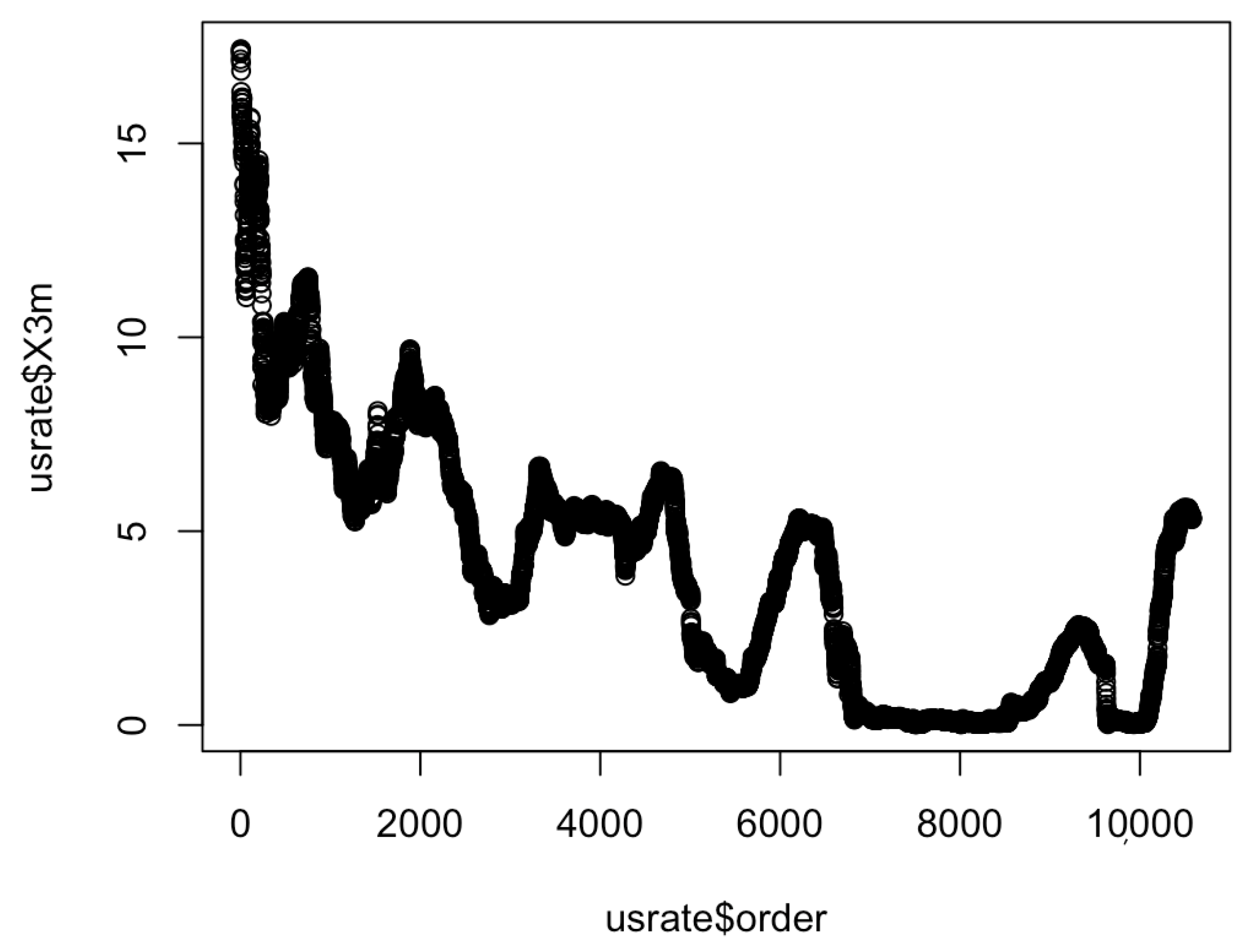
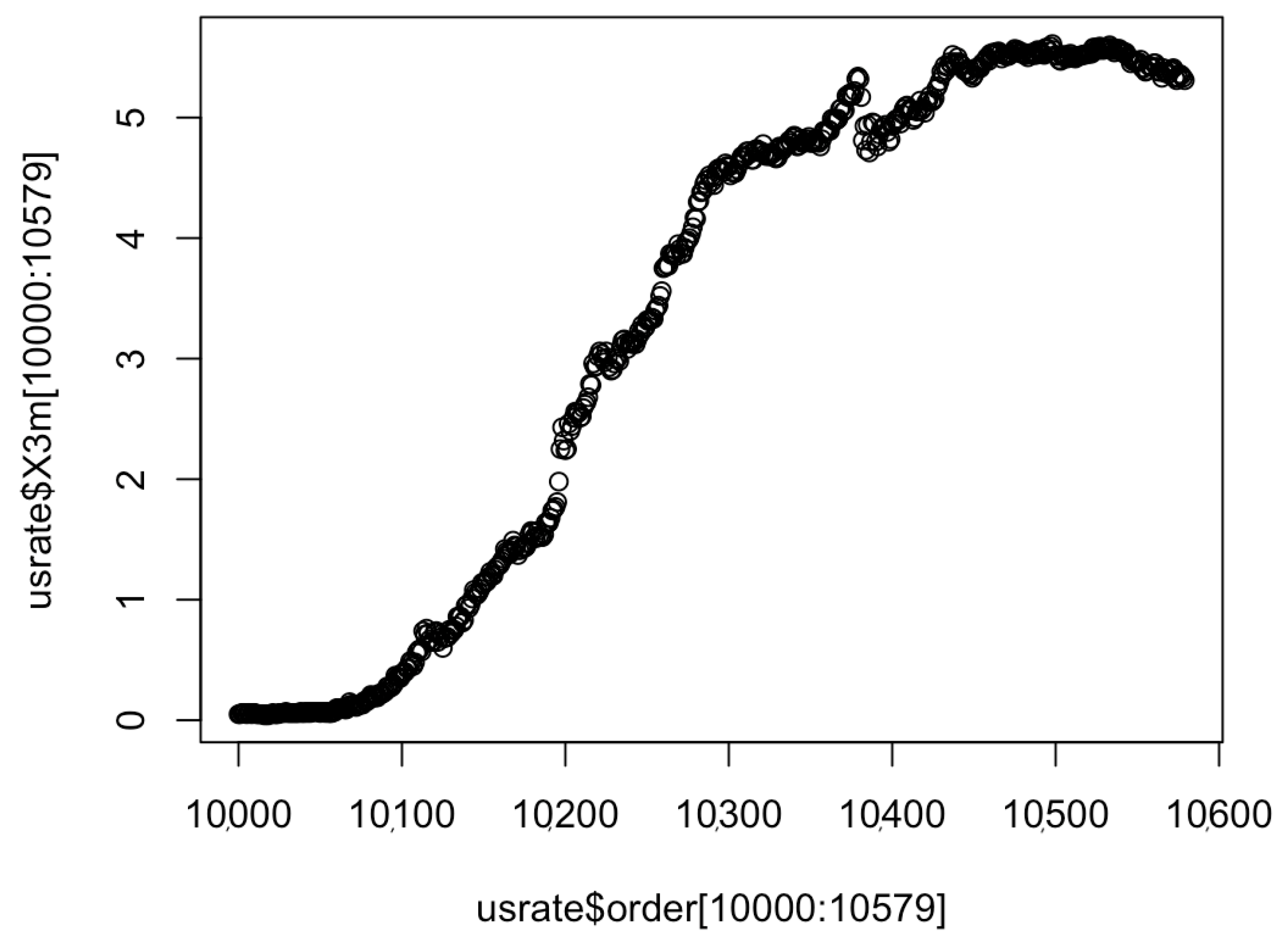
5. An Empirical Study on U.S. Treasury Rates

In this section, we apply the uncertain threshold model to estimate the term structure of a long time series of U.S. interest rates. In fact, the reason why the rates satisfy a threshold Ornstein–Uhlenbeck process was given in [40]. Consider the 3-month U.S. Treasury rate based on the Federal Reserve Bank’s H15 data set (see Figure 1), which can be downloaded from the official site of the Federal Reserve Bank.

The data are unequally spaced, as the rates are only obtained on business days. We shall adopt the convention that the equal time interval for the “daily" interest rates is $\mathrm{\Delta }t=0.046$, since one unit in time represents one month.

The tendency of the 3-month rate experiences some interruptions which can be easily detected from Figure 2. To use the approach discussed in this paper, we assume that the US interest rates follow

$$\mathrm{d}{X}_t={\rho }_1{X}_t{1}_{\{X_t<\theta \}}\mathrm{d}t+{\rho }_2{X}_t{1}_{\{X_t\ge \theta \}}\mathrm{d}t+\sigma \mathrm{d}{C}_t,$$

(18)

where ${\rho }_1,{\rho }_2,\theta ,\sigma >0$ are parameters and $C_t$ is a Liu process.

To simplify the problem, we choose $\theta =5.00$, suggested in [40], and then, estimate the parameters ${\rho }_1,{\rho }_2,\sigma$ based on the observations from 5 October 2022 to 21 December 2023 (in other words, the sample size is 580; data observed from 580 business days from 5 October 2022 to 21 December 2023). With the same arguments, we solve the system of Equation (9) accordingly. As a consequence, we have the following estimated uncertain differential equation:

$$\mathrm{d}{X}_t=0.24X_t{1}_{\{X_t<5.00\}}\mathrm{d}t+0.017X_t{1}_{\{X_t\ge 5.00\}}\mathrm{d}t+0.0021\mathrm{d}{C}_t.$$

(19)

Based on this estimated model, we estimate the 3-month U.S. interest rate for the period from 5 October 2022 to 21 December 2023. If we define that the estimated $\widehat{X_t}$ is correct once it lays in the interval $X_t\pm 5\%\ast ϵ$, where $ϵ$ is the mean error of the estimation, the rate of correctness of our model is $73.2\%$ on average.

6. Conclusions

Many models related to uncertain differential equations, especially in finance and economics, are extensively studied nowadays. This paper proposed a novel uncertain differential equation based on an uncertain threshold Ornstein–Uhlenbeck process and explored the parameter estimation problem in different cases. The estimation methods, mainly based on the moment method and maximum likelihood estimation in different scenarios discussed in this paper, are relatively easy to follow and feasible to implement. As a new model in uncertain finance, we would like to see more application of the uncertain threshold Ornstein–Uhlenbeck process in the future.

References

1. Itô, K. Stochastic integral. Proc. Imp. Acad. 1944, 20, 519–524. [Google Scholar] [CrossRef]
2. Karatzas, I.; Shreve, S. Methods of Mathematical Finance; Springer: New York, NY, USA, 1998; Volume 39. [Google Scholar]
3. Shreve, S. Stochastic Calculus for Finance II: Continuous-Time Models; Springer: New York, NY, USA, 2004; Volume 11. [Google Scholar]
4. Shreve, S. Stochastic Calculus for Finance I: The Binomial Asset Pricing Model; Springer: Pittsburgh, PA, USA, 2005. [Google Scholar]
5. Liu, B. Uncertainty Theory; Springer: Berlin/Heidelberg, Germany, 2007. [Google Scholar]
6. Liu, B. Toward uncertain finance theory. J. Uncertainty Anal. Appl. 2013, 1, 1–15. [Google Scholar] [CrossRef]
7. Liu, B. Some research problems in uncertainty theory. J. Uncertain Syst. 2009, 3, 3–10. [Google Scholar]
8. Chen, X.; Liu, B. Existence and uniqueness theorem for uncertain differential equations. Fuzzy Optim. Decis. Mak. 2010, 9, 69–81. [Google Scholar] [CrossRef]
9. Sheng, Y.; Gao, J. Exponential stability of uncertain differential equation. Soft Comput. 2016, 20, 3673–3678. [Google Scholar] [CrossRef]
10. Sheng, Y.; Wang, C. Stability in p-th moment for uncertain differential equation. J. Intell. Fuzzy Syst. 2014, 26, 1263–1271. [Google Scholar] [CrossRef]
11. Yao, K.; Ke, H.; Sheng, Y. Stability in mean for uncertain differential equation. Fuzzy Optim. Decis. Mak. 2015, 14, 365–379. [Google Scholar] [CrossRef]
12. Wang, X.; Ning, Y.; Moughal, A.; Chen, X. Adams–simpson method for solving uncertain differential equation. Appl. Math. Comput. 2015, 271, 209–219. [Google Scholar] [CrossRef]
13. Yang, X.; Ralescu, A. Adams method for solving uncertain differential equations. Appl. Math. Comput. 2015, 270, 993–1003. [Google Scholar] [CrossRef]
14. Yang, X.; Shen, Y. Runge-kutta method for solving uncertain differential equations. J. Uncertainty Anal. Appl. 2015, 3, 1–12. [Google Scholar] [CrossRef]
15. Zhang, Y.; Gao, J.; Huang, Z. Hamming method for solving uncertain differential equations. Appl. Math. Comput. 2017, 313, 331–341. [Google Scholar] [CrossRef]
16. Gao, R. Milne method for solving uncertain differential equations. Appl. Math. Comput. 2016, 274, 774–785. [Google Scholar] [CrossRef]
17. Cheng, Y.; Hu, Y.; Long, H. Generalized moment estimators for α-stable ornstein–uhlenbeck motions from discrete observations. Stat. Inference Stoch. Process. 2020, 23, 53–81. [Google Scholar] [CrossRef]
18. Hu, Y.; Song, J. Parameter estimation for fractional ornstein–uhlenbeck processes with discrete observations. In Malliavin Calculus and Stochastic Analysis: A Festschrift in Honor of David Nualart; Springer: Boston, MA, USA, 2013; pp. 427–442. [Google Scholar]
19. Wang, S.; Song, S.; Wang, Y. Skew ornstein–uhlenbeck processes and their financial applications. J. Comput. Appl. Math. 2015, 273, 363–382. [Google Scholar] [CrossRef]
20. Chen, X.; Gao, J. Uncertain term structure model of interest rate. Soft Comput. 2013, 17, 597–604. [Google Scholar] [CrossRef]
21. Yang, X.; Ke, H. Uncertain interest rate model for shanghai interbank offered rate and pricing of american swaption. Fuzzy Optim. Decis. Mak. 2023, 22, 447–462. [Google Scholar] [CrossRef]
22. Yao, K. Uncertain Differential Equations; Springer: Berlin/Heidelberg, Germany, 2016. [Google Scholar]
23. Chen, X. American option pricing formula for uncertain financial market. Int. J. Oper. Res. 2011, 8, 32–37. [Google Scholar]
24. Liu, Y.; Chen, X.; Ralescu, A. Uncertain currency model and currency option pricing. Int. J. Intell. Syst. 2015, 30, 40–51. [Google Scholar] [CrossRef]
25. Li, H.; Yang, X.; Ni, Y. Pricing of shout option in uncertain financial market. Fuzzy Optim. Decis. Mak. 2024, 23, 449–467. [Google Scholar] [CrossRef]
26. Jia, L.; Li, D.; Guo, F.; Liu, Y. Knock-out options pricing formulas in uncertain financial market with floating interest rate. Soft Comput. 2024, 1–14. [Google Scholar] [CrossRef]
27. Liu, Z.; Li, Y. Pricing and valuation of carbon swap in uncertain finance market. Fuzzy Optim. Decis. Mak. 2024, 23, 319–336. [Google Scholar] [CrossRef]
28. Sheng, Y.; Yao, K.; Chen, X. Least squares estimation in uncertain differential equations. IEEE Trans. Fuzzy Syst. 2019, 28, 2651–2655. [Google Scholar] [CrossRef]
29. Yao, K.; Liu, B. Parameter estimation in uncertain differential equations. Fuzzy Optim. Decis. Mak. 2020, 19, 1–12. [Google Scholar] [CrossRef]
30. Liu, Z. Generalized moment estimation for uncertain differential equations. Appl. Math. Comput. 2021, 392, 125724. [Google Scholar] [CrossRef]
31. Liu, Y.; Liu, B. Estimating unknown parameters in uncertain differential equation by maximum likelihood estimation. Soft Comput. 2022, 26, 2773–2780. [Google Scholar] [CrossRef]
32. Yang, X.; Liu, Y.; Park, G.-K. Parameter estimation of uncertain differential equation with application to financial market. Chaos Solitons Fractals 2020, 139, 110026. [Google Scholar] [CrossRef]
33. Li, A.; Xia, Y. Parameter estimation of uncertain differential equations with estimating functions. Soft Comput. 2024, 28, 77–86. [Google Scholar] [CrossRef]
34. Wang, J.; Gong, H.; Li, A. On weighted threshold moment estimation of uncertain differential equations with applications in interbank rates analysis. J. Ambient Intell. Humaniz. Comput. 2024, 15, 3509–3518. [Google Scholar] [CrossRef]
35. He, L.; Zhu, Y.; Gu, Y. Nonparametric estimation for uncertain differential equations. Fuzzy Optim. Decis. Mak. 2023, 22, 697–715. [Google Scholar] [CrossRef]
36. Li, A.; Xia, Y. The Nadaraya–Watson Estimation of Uncertain Differential Equations; Technical Report; Springer: Cham, Switzerland, 2023; pp. 1–20. [Google Scholar]
37. Liu, B. Fuzzy process, hybrid process and uncertain process. J. Uncertain Syst. 2008, 2, 3–16. [Google Scholar]
38. Liu, Y.; Liu, B. Residual analysis and parameter estimation of uncertain differential equations. Fuzzy Optim. Decis. Mak. 2022, 21, 513–530. [Google Scholar] [CrossRef]
39. Ye, T.; Liu, B. Uncertain hypothesis test for uncertain differential equations. Fuzzy Optim. Decis. Mak. 2022, 22, 195–211. [Google Scholar] [CrossRef]
40. Su, F.; Chan, K. Quasi-likelihood estimation of a threshold diffusion process. J. Econom. 2015, 189, 473–484. [Google Scholar] [CrossRef]
Figure 1. The 3-month U.S. Treasury rate from 1 September 1981 to 21 December 2023.
Symmetry 16 01372 g001
Figure 2. The 3-month U.S. Treasury rate in recent 580 days.
Symmetry 16 01372 g002