
Chaotic-Based Improved Henry Gas Solubility Optimization Algorithm: Application to Electric Motor Control

 , , ,
, , ,
Abstract
:1. Introduction
2. Technical Background
2.1. Henry Gas Solubility Optimization
2.1.1. Henry’s Law
2.1.2. HGSO Algorithm
2.2. Chaotic Systems
2.2.1. Duffing-Van Der Pol Chaotic System
2.2.2. Lorenz Chaotic System
2.2.3. Rucklidge Chaotic System
2.2.4. Rössler Chaotic System
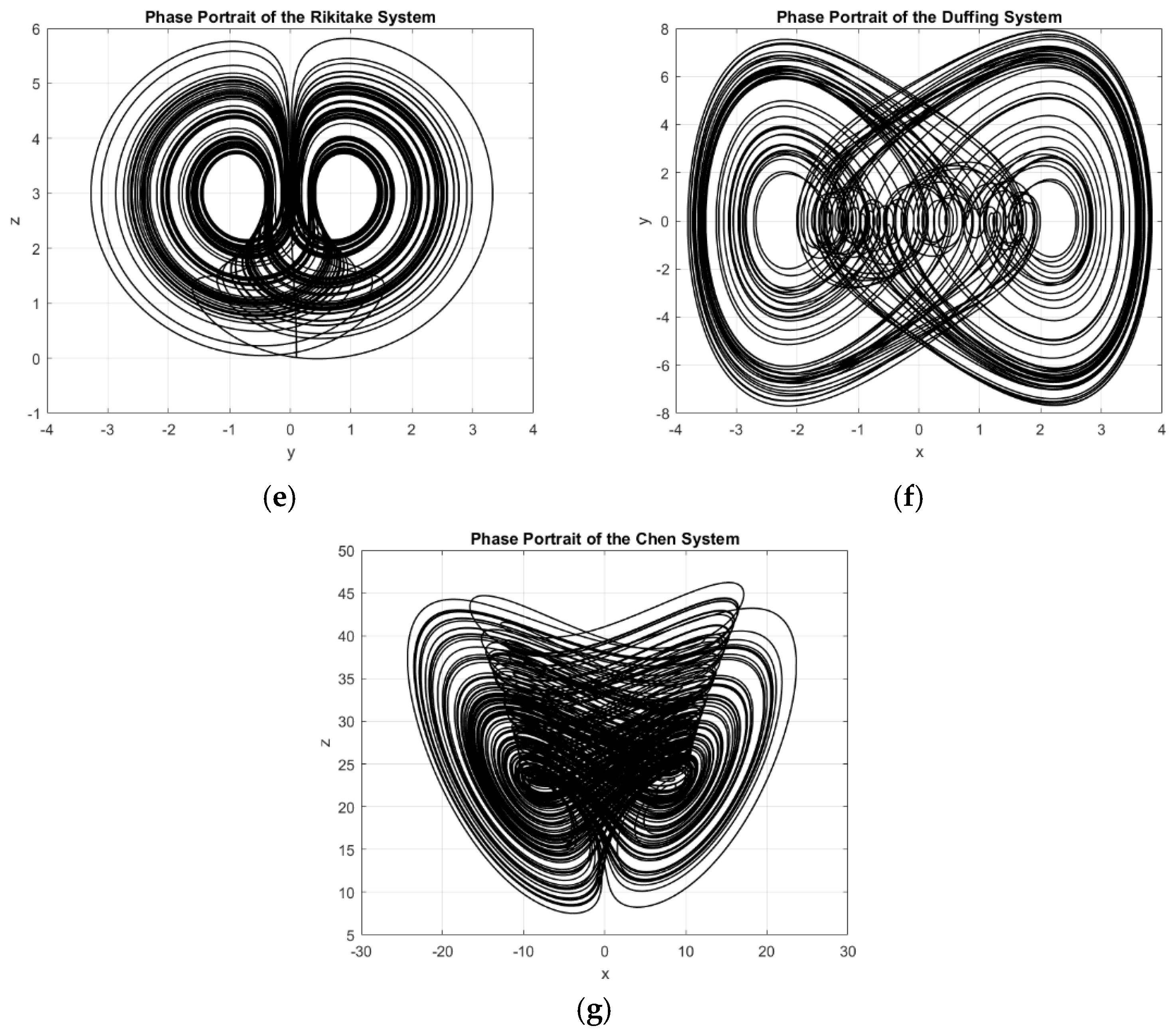
2.2.5. Rikitake Chaotic System
2.2.6. Duffing Chaotic System
2.2.7. Chen Chaotic System
2.3. NIST Tests
3. A Novel Optimization Algorithm (CHGSO)
| Algorithm 1 Pseudo-code of CHGSO algorithm [9] |
| 1: Chaotically initialization (i = 1, 2,… N), number of gas types i, , , , , and . Equations (19) and (20) 2: Divide the population agents into number of gas types (cluster) with the same Henry’s constant value (). 3: Evaluate each cluster . 4: Get the best gas in each cluster, and the best search agent . 5: while < maximum number of iterations do 6: for each search agent do 7: Chaotically update the positions of all search agents using Equation (21) 8: end for 9: Update Henry’s constant of each gas type using Equation (7) 10: Update solubility of each gas using Equation (8) 11: Rank and chaotically select number of worst agents using Equation (22). 12: Chaotically update the position of the worst agents using Equation (23). 13: Update the best gas , and the best search agent . 14: end while 15: t = t + 1 16: return |
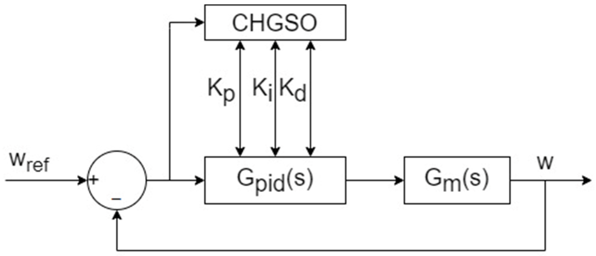
4. Optimization of PID Parameters for Speed Control of DC Motor with Proposed CHGSO Method
4.1. Results
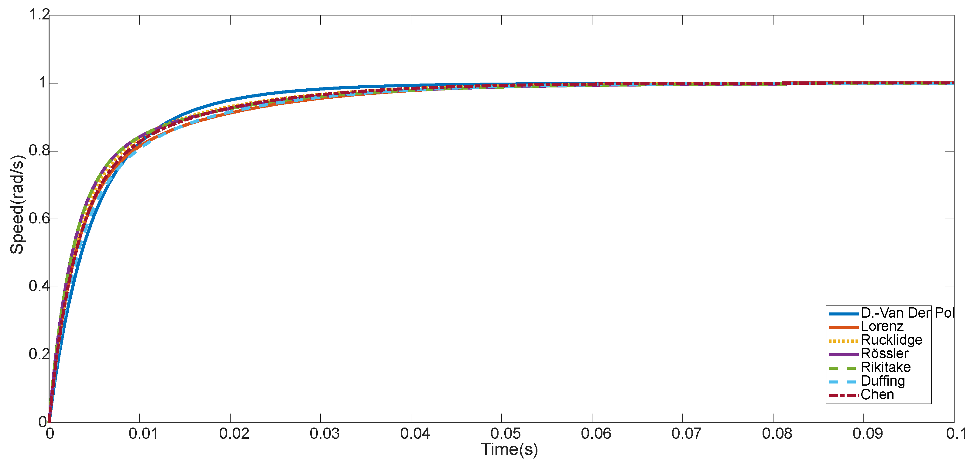
4.1.1. Simulation Results
4.1.2. Experimental Results
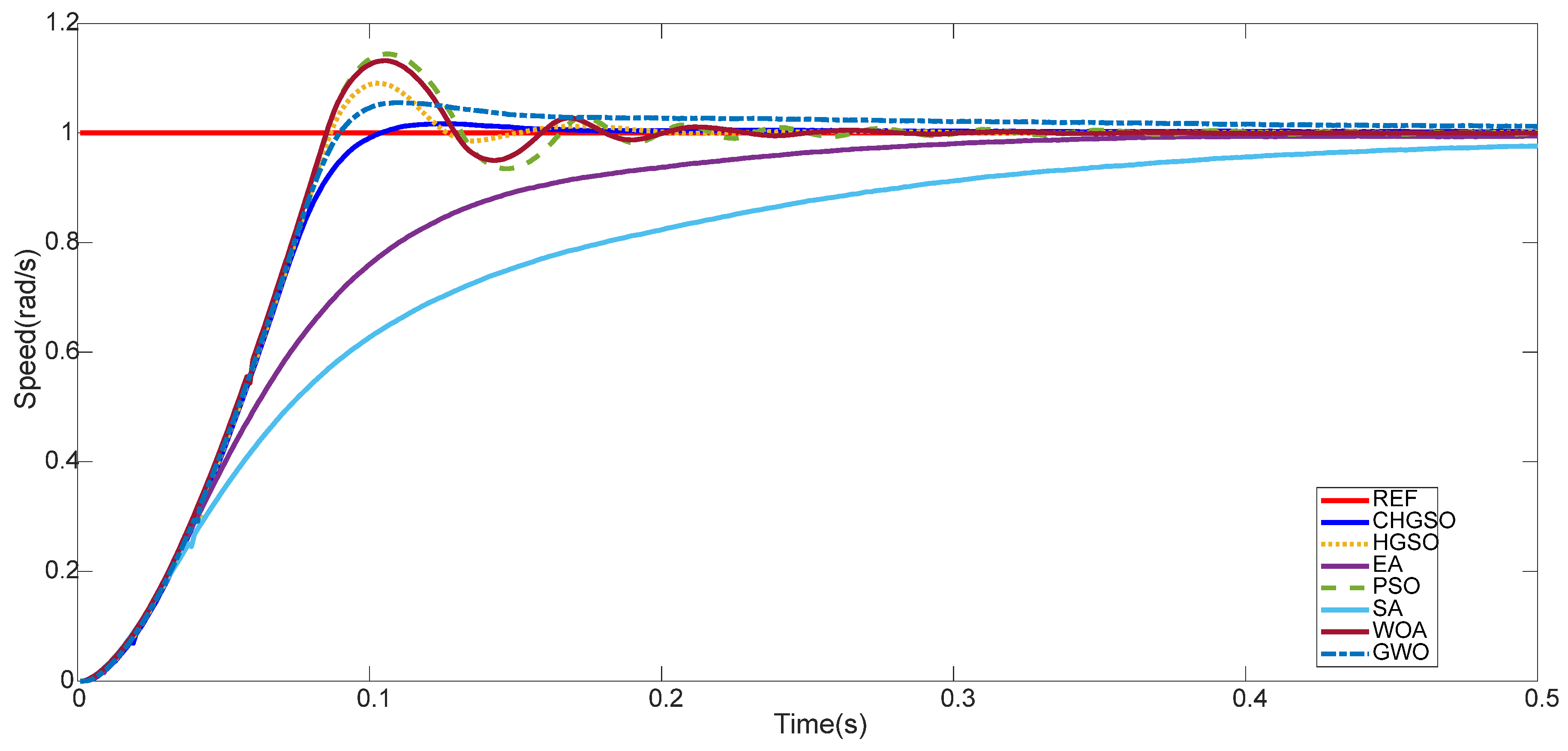
Unit Step Response of Unloaded DC Motor
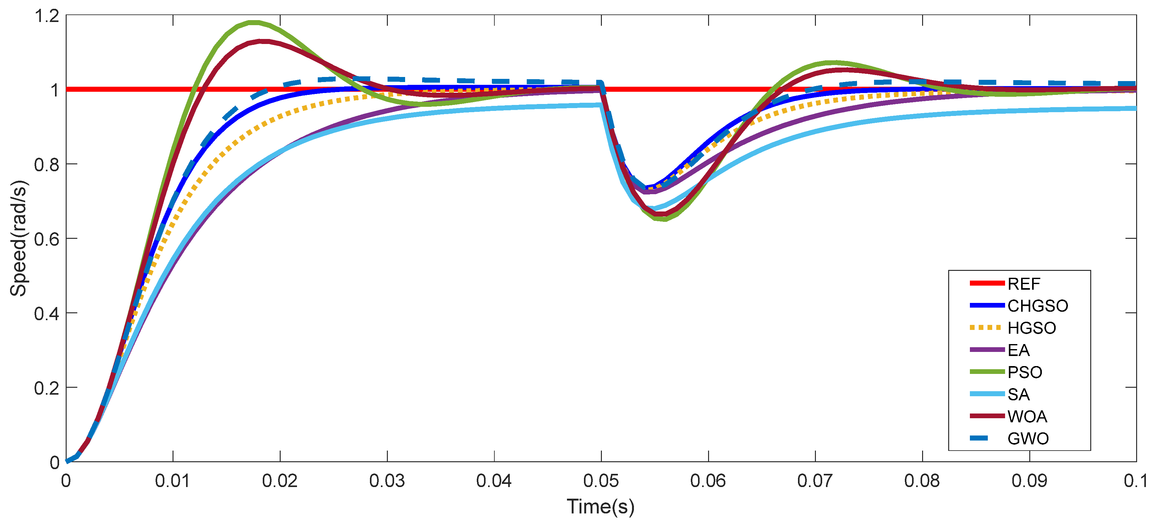
Unit Step Response of Under Load DC Motor
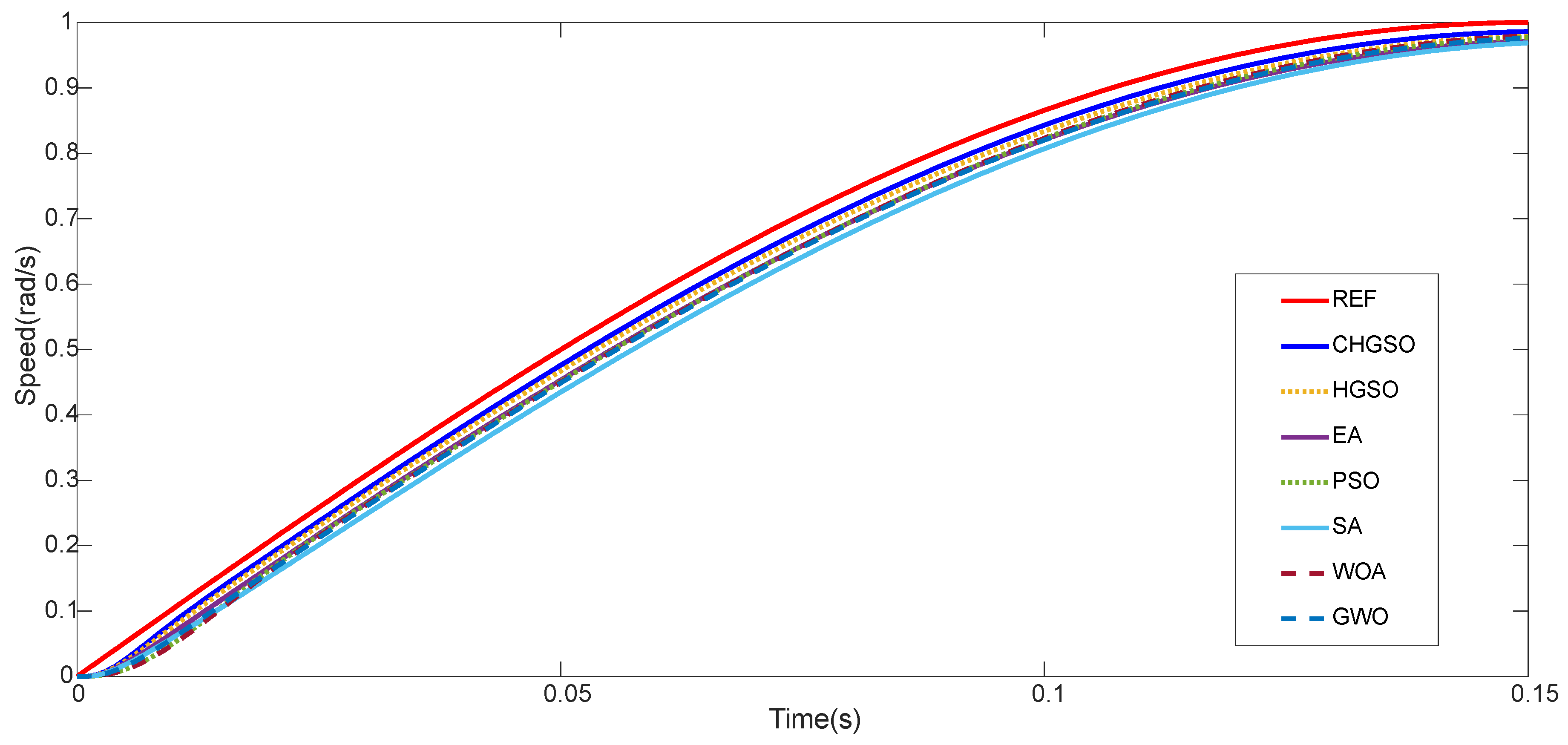
Parabolic Input Response of Unloaded DC Motor
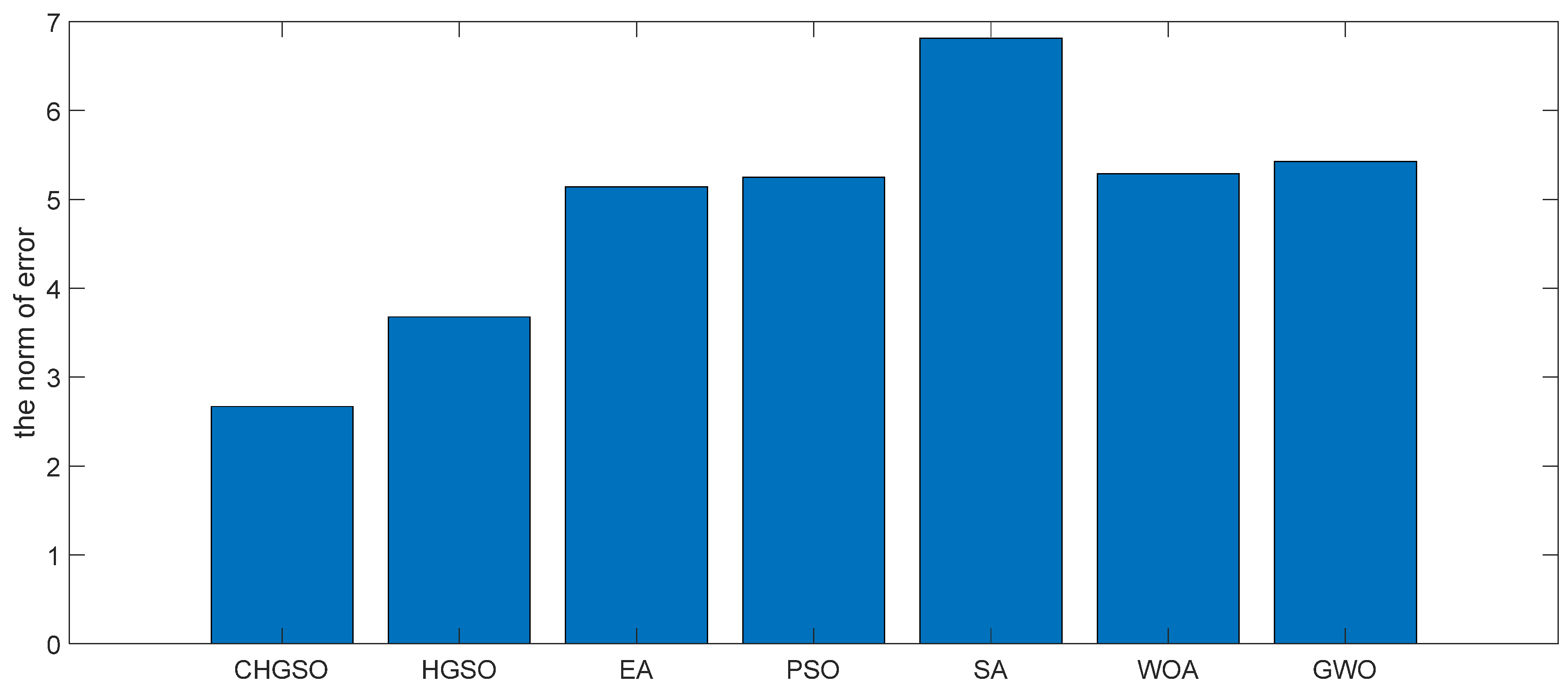
Parabolic Input Response of Under Load DC Motor
5. Conclusions
Author Contributions
Funding
Data Availability Statement
Conflicts of Interest
Appendix A

| No | Function | Name | Dim | R | Fmin |
|---|---|---|---|---|---|
| F1 | Chung Reynolds | 30 | [−100,100] | 0 | |
| F2 | Sphere | 30 | [−5.12,5.12] | 0 | |
| F3 | Powell singular 1 | 30 | [−4,5] | 0 | |
| F4 | Powell singular 2 | 30 | [−4,5] | 0 | |
| F5 | Powell Sum | 30 | [−1,1] | 0 | |
| F6 | Schwefel 2.20 | 30 | [−100,100] | 0 | |
| F7 | Schwefel 2.21 | 30 | [−100,100] | 0 | |
| F8 | Schwefel 2.22 | 30 | [−100,100] | 0 | |
| F9 | Schwefel 2.23 | 30 | [−10,10] | 0 | |
| F10 | Step 1 | 30 | [−100,100] | 0 | |
| F11 | Sum Squares | 30 | [−10,10] | 0 | |
| F12 | Ackley | 30 | [−35,35] | 0 | |
| F13 | Alpine | 30 | [−10,10] | 0 | |
| F14 | Brown | 30 | [−1,4] | 0 | |
| F15 | Cigar | 30 | [−100,100] | 0 | |
| F16 | Exponential | 30 | [−1,1] | −1 | |
| F17 | Griewank | 30 | [−600,600] | 0 | |
| F18 | Mishra 1 | 30 | [0,1] | 2 | |
| F19 | Mishra 1 | 30 | [0,1] | 2 | |
| F20 | Mishra 11 | 30 | [0,10] | 0 | |
| F21 | Quartic | 30 | [−1.28,1.28] | 0 | |
| F22 | Rastring | 30 | [−5.12,5.12] | 0 | |
| F23 | Schwefel 2.25 | 30 | [0,10] | 0 | |
| F24 | Xin−She Yang 2 | 30 | [−2π, 2π] | 0 | |
| F25 | Xin−She Yang 3 | 30 | [−20, 20] | 0 | |
| F26 | Zakharov | 30 | [−5,10] | 0 | |
| F27 | Ackley 2 | 2 | [−32,32] | −200 | |
| F28 | Bartels Conn | 2 | [−500,500] | 1 | |
| F29 | Bohachevsky 1 | 2 | [−100,100] | 0 | |
| F30 | Bohachevsky 2 | 2 | [−100,100] | 0 | |
| F31 | Bohachevsky 3 | 2 | [−100,100] | 0 | |
| F32 | Camel−Three Hump | 2 | [−5,5] | 0 | |
| F33 | Chichinadze | 2 | [−30,30] | −43.3159 | |
| F34 | Cross−in−Tray | 2 | [−10,10] | −2.06261218 | |
| F35 | ScCrossLegTable | 2 | [−10,10] | −1 | |
| F36 | Egg Crate | 2 | [−5,5] | 0 | |
| F37 | Hartman | 6 | [0,1] | −3.32236 | |
| F38 | Matyas | 2 | [−10,10] | 0 | |
| F39 | Periodic | 2 | [−10,10] | 0.9 | |
| F40 | Rump | 2 | [−500,500] | 0 | |
| F41 | Rotated Ellipse | 2 | [−500,500] | 0 | |
| F42 | Sawtoothxy | 2 | [−20,20] | 0 | |
| F43 | Scahffer1 | 2 | [−100,100] | 0 | |
| F44 | Scahffer6 | 2 | [−100,100] | 0 | |
| F45 | Stenger | 2 | [−1,4] | 0 | |
| F46 | Trecanni | 2 | [−5,5] | 0 | |
| F47 | Venter | 2 | [−50,50] | −400 |
References
- Wang, Z.; Luo, Q.; Chen, H.; Zhao, J.; Yao, L.; Zhang, J.; Chu, F. A high−accuracy intelligent fault diagnosis method for aero−engine bearings with limited samples. Comput. Ind. 2024, 159, 104099. [Google Scholar] [CrossRef]
- Alanazi, A.; Alanazi, M.; Nowdeh, S.A.; Abdelaziz, A.Y.; El−Shahat, A. An optimal sizing framework for autonomous photovoltaic/hydrokinetic/hydrogen energy system considering cost, reliability and forced outage rate using horse herd optimization. Energy Rep. 2022, 8, 7154–7175. [Google Scholar] [CrossRef]
- Zhang, Z.; Fu, Y.; Gao, K.; Pan, Q.; Huang, M. A learning−driven multi−objective cooperative artificial bee colony algorithm for distributed flexible job shop scheduling problems with preventive maintenance and transportation operations. Comput. Ind. Eng. 2024, 196, 110484. [Google Scholar] [CrossRef]
- Nowdeh, S.A.; Davoudkhani, I.F.; Moghaddam, M.H.; Najmi, E.S.; Abdelaziz, A.Y.; Ahmadi, A.; Gandoman, F.H. Fuzzy multi−objective placement of renewable energy sources in distribution system with objective of loss reduction and reliability improvement using a novel hybrid method. Appl. Soft Comput. 2019, 77, 761–779. [Google Scholar] [CrossRef]
- Jahannoush, M.; Nowdeh, S.A. Optimal designing and management of a stand−alone hybrid energy system using meta−heuristic improved sine–cosine algorithm for Recreational Center, case study for Iran country. Appl. Soft Comput. 2020, 96, 106611. [Google Scholar] [CrossRef]
- Fu, Y.; Wang, Y.; Gao, K.; Suganthan, P.N.; Huang, M. Integrated scheduling of multi−constraint open shop and vehicle routing: Mathematical model and learning−driven brain storm optimization algorithm. Appl. Soft Comput. 2024, 163, 111943. [Google Scholar] [CrossRef]
- Fu, Y.; Zhou, M.; Guo, X.; Qi, L.; Gao, K.; Albeshri, A. Multiobjective Scheduling of Energy−Efficient Stochastic Hybrid Open Shop With Brain Storm Optimization and Simulation Evaluation. IEEE Trans. Syst. Man Cybern. Syst. 2024, 54, 4260–4272. [Google Scholar] [CrossRef]
- Fu, Y.; Gao, K.; Wang, L.; Huang, M.; Liang, Y.C.; Dong, H. Scheduling stochastic distributed flexible job shops using an multi−objective evolutionary algorithm with simulation evaluation. Int. J. Prod. Res. 2024, 62, 1–18. [Google Scholar] [CrossRef]
- Hashim, F.A.; Houssein, E.H.; Mabrouk, M.S.; Al−Atabany, W.; Mirjalili, S. Henry gas solubility optimization: A novel physics−based algorithm. Future Gener. Comput. Syst. 2019, 101, 646–667. [Google Scholar] [CrossRef]
- Mirza, A.F.; Mansoor, M.; Ling, Q. A novel MPPT technique based on Henry gas solubility optimization. Energy Convers. Manag. 2020, 225, 113409. [Google Scholar] [CrossRef]
- Neggaz, N.; Houssein, E.H.; Hussain, K. An efficient henry gas solubility optimization for feature selection. Expert Syst. Appl. 2020, 152, 113364. [Google Scholar] [CrossRef]
- Ekinci, S.; İzci, D.; Hekimoğlu, B. Implementing the Henry gas solubility optimization algorithm for optimal power system stabilizer design. Electrica 2021, 21, 250–258. [Google Scholar] [CrossRef]
- Mousakazemi, S.M.H. Henry gas solubility optimization for control of a nuclear reactor: A case study. Nucl. Eng. Technol. 2022, 54, 940–947. [Google Scholar] [CrossRef]
- Yıldız, B.S.; Pholdee, N.; Panagant, N.; Bureerat, S.; Yildiz, A.R.; Sait, S.M. A novel chaotic Henry gas solubility optimization algorithm for solving real−world engineering problems. Eng. Comput. 2022, 38, 871–883. [Google Scholar] [CrossRef]
- Agarwal, R.; Shekhawat, N.S.; Luhach, A.K. Automated classification of soil images using chaotic Henry’s gas solubility optimization: Smart agricultural system. Microprocess. Microsyst. 2021, in press. [Google Scholar] [CrossRef]
- Karasu, S.; Altan, A. Crude oil time series prediction model based on LSTM network with chaotic Henry gas solubility optimization. Energy 2022, 242, 122964. [Google Scholar] [CrossRef]
- Mohammadi, D.; Abd Elaziz, M.; Moghdani, R.; Demir, E.; Mirjalili, S. Quantum Henry gas solubility optimization algorithm for global optimization. Eng. Comput. 2022, 38, 2329–2348. [Google Scholar] [CrossRef]
- Chang, W.D. PID control for chaotic synchronization using particle swarm optimization. Chaos 2009, 39, 910–917. [Google Scholar] [CrossRef]
- Rastogi, A.; Tiwari, P. Optimal tuning of fractional order PID controller for DC motor speed control using particle swarm optimization. Int. J. Soft Comput. Eng. 2013, 3, 150–157. [Google Scholar]
- Iruthayarajan, M.W.; Baskar, S. Evolutionary algorithms based design of multivariable PID controller. Expert Syst. Appl. 2009, 36, 9159–9167. [Google Scholar] [CrossRef]
- Hung, M.H.; Shu, L.S.; Ho, S.J.; Hwang, S.F.; Ho, S.Y. A novel intelligent multiobjective simulated annealing algorithm for designing robust PID controllers. Syst. Man Cybern. Part A Syst. Humans 2008, 38, 319–330. [Google Scholar] [CrossRef]
- Pareek, S.; Kishnani, M.; Gupta, R. Application of artificial bee colony optimization for optimal PID tuning. In Proceedings of the 2014 International Conference on Advances in Engineering & Technology Research (ICAETR−2014), Unnao, India, 1–2 August 2014; pp. 1–5. [Google Scholar] [CrossRef]
- El−Telbany, M.E. Tuning PID controller for DC motor: An artificial bees optimization approach. Int. J. Comput. Appl. 2013, 77, 18–21. [Google Scholar] [CrossRef]
- Liao, W.; Hu, Y.; Wang, H. Optimization of PID control for DC motor based on artificial bee colony algorithm. In Proceedings of the 2014 International Conference on Advanced Mechatronic Systems, Kumamoto, Japan, 10–12 August 2014; pp. 23–27. [Google Scholar] [CrossRef]
- Achanta, R.K.; Pamula, V.K. DC motor speed control using PID controller tuned by jaya optimization algorithm. In Proceedings of the 2017 IEEE International Conference on Power, Control, Signals and Instrumentation Engineering (ICPCSI), Chennai, India, 21–22 September 2017; pp. 983–987. [Google Scholar] [CrossRef]
- Khalilpour, M.; Razmjooy, N.; Hosseini, H.; Moallem, P. Optimal control of DC motor using invasive weed optimization (IWO) algorithm. In Proceedings of the Majlesi Conference on Electrical Engineering, Majlesi New Town, Isfahan, Iran, 25 August 2011. [Google Scholar]
- Aziz, M.S.I.; Nawawi, S.W.; Sudin, S.; Wahab, N.A.; Faramarzi, M.; Yusof, M.A.M. Gravitational search algorithm optimization for PID controller tuning in waste−water treatment process. J. Teknol. 2015, 73, 103–109. [Google Scholar] [CrossRef]
- Izci, D.; Ekinci, S.; Demirören, A.; Hedley, J. HHO algorithm based PID controller design for aircraft pitch angle control system. In Proceedings of the 2020 International Congress on Human−Computer Interaction, Optimization and Robotic Applications (HORA), Ankara, Turkey, 26–28 June 2020; pp. 1–6. [Google Scholar] [CrossRef]
- Elbayomy, K.M.; Zongxia, J.; Huaqing, Z. PID controller optimization by GA and its performances on the electro−hydraulic servo control system. Chin. J. Aeronaut. 2008, 21, 378–384. [Google Scholar] [CrossRef]
- Zahir, A.M.; Alhady, S.S.N.; Wahab, A.A.A.; Ahmad, M.F. Objective functions modification of GA optimized PID controller for brushed DC motor. Int. J. Electr. Comput. Eng. 2020, 10, 2426. [Google Scholar] [CrossRef]
- Loucif, F.; Kechida, S.; Sebbagh, A. Whale optimizer algorithm to tune PID controller for the trajectory tracking control of robot manipulator. J. Braz. Soc. Mech. Sci. Eng. 2020, 42, 1. [Google Scholar] [CrossRef]
- Awrejcewicz, J.; Mrozowski, J. Bifurcations and chaos of a particular van der Pol−duffing oscillator. J. Sound Vib. 1989, 132, 89–100. [Google Scholar] [CrossRef]
- Lazzús, J.A.; Rivera, M.; López−Caraballo, C.H. Parameter estimation of Lorenz chaotic system using a hybrid swarm intelligence algorithm. Phys. Lett. A 2016, 380, 1164–1171. [Google Scholar] [CrossRef]
- Kocamaz, U.E.; Uyaroğlu, Y. Controlling Rucklidge chaotic system with a single controller using linear feedback and passive control methods. Nonlinear Dyn. 2014, 75, 63–72. [Google Scholar] [CrossRef]
- Rafikov, M.; Balthazar, J.M. On an optimal control design for Rössler system. Phys. Lett. A 2004, 333, 241–245. [Google Scholar] [CrossRef]
- Khan, A.; Trikha, P. Compound difference anti−synchronization between chaotic systems of integer and fractional order. SN Appl. Sci. 2019, 1, 1–13. [Google Scholar] [CrossRef]
- Ueda, Y. Randomly transitional phenomena in the system governed by Duffing’s equation. J. Stat. Phys. 1979, 20, 181–196. [Google Scholar] [CrossRef]
- Wang, J.; Zhou, B.; Zhou, S. An improved cuckoo search optimization algorithm for the problem of chaotic systems parameter estimation. Comput. Intell. Neurosci. 2016, 2016, 1–8. [Google Scholar] [CrossRef]
- Bassham, L.E., III; Rukhin, A.L.; Soto, J.; Nechvatal, J.R.; Smid, M.E.; Barker, E.B.; Vo, S. A Statistical Test Suite for Random and Pseudorandom Number Generators for Cryptographic Applications; National Institute of Standards & Technology: Gaithersburg, MD, USA, 2010. [Google Scholar]
- Jenkinson, O. Ergodic optimization in dynamical systems. Ergod. Theory Dyn. Syst. 2019, 39, 2593–2618. [Google Scholar] [CrossRef]
- Shi, Y.; Eberhart, R.C. A modified particle swarm optimizer. In Proceedings of the IEEE International Conference on Evolutionary Computation, Anchorage, AK, USA, 4–9 May 1998; pp. 69–73. [Google Scholar]
- Mirjalili, S.; Lewis, A. The whale optimization algorithm. Adv. Eng. Softw. 2016, 95, 51–67. [Google Scholar] [CrossRef]
- Van Laarhoven, P.J.; Aarts, E.H.; van Laarhoven, P.J.; Aarts, E.H. Simulated Annealing; Springer: Berlin/Heidelberg, Germany, 1987; pp. 7–15. [Google Scholar]
- Beyer, H.G.; Schwefel, H.P. Evolution strategies–a comprehensive introduction. Nat. Comput. 2002, 1, 3–52. [Google Scholar] [CrossRef]
- Mirjalili, S.; Mirjalili, S.M.; Lewis, A. Grey wolf optimizer. Adv. Eng. Softw. 2014, 69, 46–61. [Google Scholar] [CrossRef]


| Duffing-Van Der Pol | Lorenz | Rössler | Rikitake | Duffing | Chen | Rucklidge | |
|---|---|---|---|---|---|---|---|
| Frequency (monobit) test | Passed | Passed | Passed | Passed | Passed | Passed | Passed |
| Block frequency test | Passed | Passed | Passed | Passed | Passed | Passed | Passed |
| Cumulative sum test | Passed | Passed | Passed | Passed | Passed | Passed | Passed |
| Runs test | Passed | Passed | Passed | Passed | Passed | Passed | Passed |
| Longest run test | Passed | Passed | Passed | Passed | Passed | Passed | Passed |
| Binary matrix rank test | Passed | Passed | Passed | Passed | Passed | Passed | Passed |
| Discrete Fourier transform test | Passed | Passed | Passed | Passed | Passed | Passed | Passed |
| Non overlapping templates test | Passed | Passed | Passed | Passed | Passed | Failed | Failed |
| Overlapping templates test | Passed | Passed | Passed | Passed | Passed | Passed | Passed |
| Maurer’s universal statistical test | Passed | Passed | Passed | Passed | Passed | Passed | Passed |
| Approximate entropy test | Passed | Passed | Passed | Passed | Passed | Passed | Passed |
| Random excursions test | Passed | Passed | Passed | Passed | Passed | Passed | Passed |
| Random excursions variant test | Passed | Passed | Passed | Passed | Passed | Passed | Passed |
| Serial test | Passed | Passed | Passed | Passed | Passed | Passed | Passed |
| Linear complexity test | Passed | Passed | Passed | Passed | Passed | Passed | Passed |
| CHGSO (proposed method) | Number of iterations: 200 Number of gas particles: 30 Number of clusters: 5 M1 = 0.1, M2 = 0.2, L1 = 0.005, l2 = 100, l3 = 0.01, a, b, k = 1, e = 0.05 |
| HGSO | Number of iterations: 200 Number of gas particles: 30 Number of clusters: 5 M1 = 0.1, M2 = 0.2, L1 = 0.005, l2 = 100, l3 = 0.01, a, b, k = 1, e = 0.05 |
| QHGSO | Number of iterations: 200 Number of gas particles: 30 Number of clusters: N/A M1 = 0.1, M2 = 0.2, L1 = 0.005, l2 = 100, l3 = 0.01, a, b, k = 1, e = 0.05 |
| PSO | Number of iterations: 200 Number of swarm: 30 C1 = 2.1, C2 = 2.1 |
| EA | Number of iterations: 200 Number of parents: 20 Number of children: 4 |
| GWO | Number of iterations: 200 Number of wolves: 30 |
| SA | Number of iterations: 200 Number of materials: 30 Cooling rate: 0.98 |
| WOA | Number of iterations: 200 Number of whales: 30 |
| Fmin | CHGSO | HGSO | QHGSO | PSO | EA | GWO | SA | WOA | ||
|---|---|---|---|---|---|---|---|---|---|---|
| F1 | 0.00 × 100 | MEAN | 0.00 × 100 | 4.13 × 10−158 | 0.00 × 100 | 7.62 × 101 | 4.35 × 10⁹ | 1.26 × 10⁻¹⁶ | 2.00×10⁹ | 9.28 × 10−43 |
| STD | 0.00 × 100 | 8.13 × 10−159 | 0.00 × 100 | 1.31 × 10² | 9.81 × 10⁸ | 3.87 × 10⁻¹⁶ | 3.79×10⁸ | 3.39 × 10−42 | ||
| F2 | 0.00 × 100 | MEAN | 0.00 × 100 | 1.60 × 10−81 | 0.00 × 100 | 8.18 × 100 | 1.51 × 10⁻³ | 2.64 × 10⁻¹¹ | 1.22×10² | 1.51 × 10⁻²⁴ |
| STD | 0.00 × 100 | 1.12 × 10−80 | 0.00 × 100 | 5.71 × 100 | 9.07 × 10⁻⁴ | 3.62 × 10⁻¹¹ | 1.07×101 | 7.03 × 10⁻²⁴ | ||
| F3 | 0.00 × 100 | MEAN | 0.00 × 100 | 7.72 × 10−80 | 0.00 × 100 | 5.74 × 10⁴ | 1.10 × 10² | 2.06 × 10⁻² | 5.96×10⁴ | 1.92 × 10⁻²⁴ |
| STD | 0.00 × 100 | 5.37 × 10−79 | 0.00 × 100 | 6.40 × 10⁴ | 6.17 × 101 | 3.4 × 10⁻² | 3.72×10⁴ | 1.21 × 10⁻²³ | ||
| F4 | 0.00 × 100 | MEAN | 0.00 × 100 | 1.03 × 10−79 | 0.00 × 100 | 7.61 × 10⁴ | 8.21 × 10⁻¹ | 2.01 × 10⁻⁷ | 1.50×10⁻¹ | 4.39 × 10⁻²⁴ |
| STD | 0.00 × 100 | 4.35 × 10−79 | 0.00 × 100 | 1.04 × 10⁵ | 5.96 × 10⁻¹ | 2.76 × 10⁻⁷ | 6.10×10⁻² | 2.93 × 10⁻²³ | ||
| F5 | 0.00 × 100 | MEAN | 0.00 × 100 | 1.87 × 10−125 | 0.00 × 100 | 5.00 × 10¹⁵ | 3.45 × 10⁻⁶ | 4.02 × 10−37 | 9.05×10³ | 2.16 × 10−36 |
| STD | 0.00 × 100 | 1.09 × 10−124 | 0.00 × 100 | 3.11 × 10¹⁶ | 1.48 × 10⁻⁶ | 1.69 × 10−37 | 1.34×10³ | 1.03 × 10⁻³⁵ | ||
| F6 | 0.00 × 100 | MEAN | 0.00 × 100 | 6.82 × 10−41 | 0.00 × 100 | 5.38 × 100 | 9.28 × 100 | 5.52 × 10⁻⁵ | 9.25×10² | 1.94 × 10⁻¹⁶ |
| STD | 0.00 × 100 | 3.40 × 10−40 | 0.00 × 100 | 2.14 × 100 | 5.21 × 100 | 2.98 × 10⁻⁵ | 5.36×101 | 4.61 × 10⁻¹⁶ | ||
| F7 | 0.00 × 100 | MEAN | 0.00 × 100 | 5.43 × 10−40 | 0.00 × 100 | 8.47 × 100 | 2.17 × 101 | 3.08 × 10⁻² | 7.48×101 | 6.07 × 101 |
| STD | 0.00 × 100 | 2.75 × 10−39 | 0.00 × 100 | 1.49 × 100 | 8.44 × 100 | 2.01 × 10⁻² | 2.48×100 | 2.78 × 101 | ||
| F8 | 0.00 × 100 | MEAN | 0.00 × 100 | 8.82 × 10−41 | 0.00 × 100 | 1.29 × 10² | 6.09 × 1028 | 8.71 × 10⁻⁵ | 1.50×1037 | 1.35 × 10⁻¹⁶ |
| STD | 0.00 × 100 | 3.91 × 10−40 | 0.00 × 100 | 1.87 × 10² | 3.37 × 1029 | 4.77 × 10⁻⁵ | 3.47×1037 | 4.05 × 10⁻¹⁶ | ||
| F9 | 0.00 × 100 | MEAN | 0.00 × 100 | 0.00 × 100 | 0.00 × 100 | 6.95 × 10⁷ | 1.19 × 10⁹ | 4.61 × 10⁻³⁰ | 1.66×10⁹ | 3.70 × 10−43 |
| STD | 0.00 × 100 | 0.00 × 100 | 0.00 × 100 | 1.28 × 10⁸ | 8.54 × 10⁸ | 1.92 × 10⁻²⁹ | 6.23×10⁸ | 2.60 × 10−42 | ||
| F10 | 0.00 × 100 | MEAN | 0.00 × 100 | −1.79 × 10³ | 0.00 × 100 | −3.00 × 10³ | −2.96 × 10³ | −2.77 × 10³ | −2.09×10³ | −3.00 × 10³ |
| STD | 0.00 × 100 | 2.21 × 10² | 0.00 × 100 | 4.80 × 10⁻¹ | 3.55 × 101 | 1.48 × 10² | 5.02×101 | 0.00 × 100 | ||
| F11 | 0.00 × 100 | MEAN | 0.00 × 100 | 1.89 × 10−77 | 0.00 × 100 | 8.48 × 101 | 2.94 × 100 | 9.47 × 10⁻¹⁰ | 6.04×10³ | 2.65 × 10⁻²³ |
| STD | 0.00 × 100 | 1.28 × 10−76 | 0.00 × 100 | 7.17 × 101 | 2.56 × 100 | 1.24 × 10⁻⁹ | 6.11×10² | 8.28 × 10⁻²³ | ||
| F12 | 0.00 × 100 | MEAN | 8.88 × 10⁻¹⁶ | 8.88 × 10⁻¹⁶ | 8.70 × 100 | 2.03 × 101 | 1.41 × 101 | 1.98 × 10⁻⁵ | 2.03×101 | 8.61 × 10⁻¹³ |
| STD | 2.06 × 10⁻³¹ | 8.96 × 10⁻³¹ | 6.12 × 100 | 3.31 × 100 | 8.19 × 100 | 7.83 × 10⁻⁶ | 1.73×10⁻¹ | 1.93 × 10⁻¹² | ||
| F13 | 0.00 × 100 | MEAN | 0.00 × 100 | 9.43 × 10−43 | 8.65 × 10⁻¹ | 4.80 × 101 | 4.11 × 100 | 4.17 × 10⁻³ | 4.61×101 | 5.10 × 10⁻¹ |
| STD | 4.13 × 10−139 | 4.44 × 10−42 | 2.31 × 100 | 3.10 × 101 | 2.02 × 100 | 1.76 × 10⁻³ | 2.97×100 | 3.61 × 100 | ||
| F14 | 0.00 × 100 | MEAN | 0.00 × 100 | 1.51 × 10−81 | 7.17 × 10² | 1.56 × 10⁻⁹ | 1.94 × 10⁻³ | 1.97 × 10⁻¹¹ | 6.81×101 | 6.56 × 10⁻²⁶ |
| STD | 0.00 × 100 | 9.48 × 10−81 | 1.90 × 10³ | 1.07 × 10⁻⁹ | 1.90 × 10⁻³ | 2.97 × 10⁻¹¹ | 1.44×101 | 2.06 × 10⁻²⁵ | ||
| F15 | 0.00 × 100 | MEAN | 0.00 × 100 | 2.62 × 10−73 | 9.98 × 10⁻¹ | 4.49 × 10⁶ | 6.58 × 10¹⁰ | 5.26 × 10⁻³ | 4.29×10¹⁰ | 5.28 × 10⁻¹⁵ |
| STD | 0.00 × 100 | 1.56 × 10−72 | −9.98 × 10⁻¹ | 2.61 × 10⁶ | 6.74 × 10⁹ | 4.84 × 10⁻³ | 3.76×10⁹ | 3.53 × 10⁻¹⁴ | ||
| F16 | −1.00 × 100 | MEAN | −1.00 × 100 | −1.00 × 100 | 1.48 × 100 | −1.00 × 100 | −1.00 × 100 | −1.00 × 100 | −1.03×10⁻¹ | −1.00 × 100 |
| STD | 0.00 × 100 | 0.00 × 100 | 1.49 × 100 | 0.00 × 100 | 2.25 × 10⁻⁵ | 0.00 × 100 | 1.26×10⁻² | 0.00 × 100 | ||
| F17 | 0.00 × 100 | MEAN | 0.00 × 100 | 0.00 × 100 | 1.61 × 101 | 3.66 × 10⁻¹ | 9.15 × 10⁻¹ | 1.18 × 10⁻² | 3.99×10² | 7.20 × 10⁻³ |
| STD | 0.00 × 100 | 0.00 × 100 | 1.36 × 101 | 2.29 × 10⁻¹ | 1.28 × 10⁻¹ | 1.50 × 10⁻² | 3.75×101 | 5.09 × 10⁻² | ||
| F18 | 2.00 × 100 | MEAN | 2.00 × 100 | 1.89 × 101 | 4.35 × 100 | −1.54 × 10⁶ | 1.11 × 10⁷ | 8.10 × 100 | 3.80×10¹⁰ | 2.00 × 100 |
| STD | 0.00 × 100 | 8.87 × 101 | 1.78 × 101 | 8.96 × 10⁶ | 6.72 × 10⁷ | 1.39 × 101 | 5.58×10¹⁰ | 0.00 × 100 | ||
| F19 | 2.00 × 100 | MEAN | 2.00 × 100 | 4.84 × 101 | 7.35 × 10⁻¹⁹ | −6.49 × 10⁶ | 3.89 × 10⁶ | 2.30 × 101 | 7.79×10¹⁰ | 2.00 × 100 |
| STD | 0.00 × 100 | 3.03 × 10² | 4.08 × 10⁻¹⁷ | 4.58 × 10⁷ | 2.56 × 10⁷ | 3.85 × 101 | 1.54×10¹¹ | 0.00 × 100 | ||
| F20 | 0.00 × 100 | MEAN | 0.00 × 100 | 0.00 × 100 | 4.16 × 10⁻¹ | 2.89 × 10⁻⁵ | 9.01 × 10⁻¹² | 5.38 × 10⁻⁸ | 1.37×10⁻¹ | 0.00 × 100 |
| STD | 0.00 × 100 | 0.00 × 100 | 2.56 × 10⁻¹ | 9.79 × 10⁻⁵ | 9.31 × 10⁻¹² | 4.00 × 10⁻⁸ | 2.80×10⁻² | 0.00 × 100 | ||
| F21 | 0.00 × 100 | MEAN | 6.57 × 10⁻⁶ | 3.01 × 10⁻⁴ | 6.56 × 101 | 1.71 × 10³ | 3.03 × 10⁻¹ | 7.10 × 10⁻³ | 5.53×101 | 1.18 × 10⁻² |
| STD | 1.63 × 10⁻⁵ | 2.79 × 10⁻⁴ | 4.64 × 101 | 1.42 × 10³ | 1.16 × 10⁻¹ | 3.61 × 10⁻³ | 7.56×100 | 1.28 × 10⁻² | ||
| F22 | 0.00 × 100 | MEAN | 0.00 × 100 | 0.00 × 100 | 2.69 × 10² | 2.20 × 10² | 1.08 × 10² | 1.36 × 101 | 3.58×10² | 2.55 × 100 |
| STD | 0.00 × 100 | 0.00 × 100 | 1.95 × 10² | 4.79 × 101 | 2.35 × 101 | 1.08 × 101 | 1.65×101 | 1.78 × 101 | ||
| F23 | 0.00 × 100 | MEAN | 5.14 × 10⁻¹ | 1.61 × 101 | 3.27 × 10⁻⁹ | 2.20 × 10² | 8.74 × 10⁻² | 5.15 × 100 | 1.06×10⁴ | 1.61 × 101 |
| STD | 4.17 × 100 | 2.32 × 100 | 1.03 × 10⁻⁹ | 4.79 × 101 | 5.83 × 10⁻² | 1.93 × 100 | 1.96×10³ | 6.44 × 100 | ||
| F24 | 0.00 × 100 | MEAN | 4.17 × 10⁻¹² | 3.15 × 10⁻¹¹ | 1.94 × 10⁻⁸ | 2.91 × 10⁻⁴ | 1.91 × 10⁻¹¹ | 1.61 × 10⁻⁷ | 1.48×10⁻⁵ | 5.72 × 10⁻¹² |
| STD | 1.07 × 10⁻¹¹ | 6.19 × 10⁻¹³ | 1.94 × 10⁻⁸ | 3.78 × 10⁻⁴ | 1.22 × 10⁻¹¹ | 5.58 × 10⁻⁷ | 1.34×10⁻⁵ | 3.25 × 10⁻¹² | ||
| F25 | 0.00 × 100 | MEAN | 4.34 × 10−236 | 4.34 × 10−232 | 2.43 × 10² | 0.00 × 100 | 1.07 × 10−97 | 1.27 × 10−103 | 1.72×10−53 | −1.40 × 10⁻¹ |
| STD | 3.89 × 10⁻¹ | 0.00 × 100 | 9.38 × 101 | 0.00 × 100 | 7.60 × 10−97 | 8.97 × 10−103 | 8.26×10−53 | 3.51 × 10⁻¹ | ||
| F26 | 0.00 × 100 | MEAN | 0.00 × 100 | 1.49 × 10−75 | 9.38 × 101 | 1.15 × 10⁹ | 2.94 × 10¹⁰ | 2.90 × 10⁻⁹ | 3.86×10⁸ | 1.02 × 10⁻²¹ |
| STD | 0.00 × 100 | 1.06 × 10−74 | −2.00 × 10² | 2.10 × 10⁹ | 3.49 × 10¹⁰ | 4.12 × 10⁻⁹ | 1.39×10⁸ | 4.66 × 10⁻²¹ | ||
| F27 | −2.00 × 10² | MEAN | −2.00 × 10² | −2.00 × 10² | −2.00 × 10² | −2.00 × 10² | −2.00 × 10² | −2.00 × 10² | −1.98×10² | −2.00 × 10² |
| STD | 0.00 × 100 | 0.00 × 100 | 0.00 × 100 | 0.00 × 100 | 0.00 × 100 | 0.00 × 100 | 9.13×10⁻¹ | 0.00 × 100 | ||
| F28 | 1.00 × 100 | MEAN | 1.00 × 100 | 1.00 × 100 | 1.00 × 100 | 1.00 × 100 | 1.00 × 100 | 1.00 × 100 | 8.40×101 | 1.00 × 100 |
| STD | 0.00 × 100 | 0.00 × 100 | 0.00 × 100 | 0.00 × 100 | 7.99 × 10⁻⁶ | 0.00 × 100 | 6.57×101 | 0.00 × 100 | ||
| F29 | 0.00 × 100 | MEAN | 0.00 × 100 | 0.00 × 100 | 0.00 × 100 | 0.00 × 100 | 8.88 × 10⁻¹⁸ | 0.00 × 100 | 4.25×100 | 4.44 × 10⁻¹⁸ |
| STD | 0.00 × 100 | 0.00 × 100 | 0.00 × 100 | 0.00 × 100 | 6.28 × 10⁻¹⁷ | 0.00 × 100 | 3.43×100 | 3.14 × 10⁻¹⁷ | ||
| F30 | 0.00 × 100 | MEAN | 1.80 × 10⁻¹ | 1.80 × 10⁻¹ | 1.80 × 10⁻¹ | 1.80 × 10⁻¹ | 1.80 × 10⁻¹ | 1.80 × 10⁻¹ | 4.93×100 | 1.92 × 10⁻¹ |
| STD | 2.90 × 10⁻¹⁷ | 1.12 × 10⁻¹⁶ | 0.00 × 100 | 1.12 × 10⁻¹⁶ | 1.12 × 10⁻¹⁶ | 1.12 × 10⁻¹⁶ | 3.72×100 | 4.61 × 10⁻² | ||
| F31 | 0.00 × 100 | MEAN | 0.00 × 100 | 0.00 × 100 | 0.00 × 100 | 7.77 × 10⁻¹⁸ | 0.00 × 100 | 0.00 × 100 | 2.93×100 | 2.05 × 10⁻⁴ |
| STD | 0.00 × 100 | 0.00 × 100 | 0.00 × 100 | 2.25 × 10⁻¹⁷ | 0.00 × 100 | 0.00 × 100 | 2.67×100 | 5.25 × 10⁻⁴ | ||
| F32 | 0.00 × 100 | MEAN | 0.00 × 100 | 3.79 × 10−110 | 0.00 × 100 | 9.42 × 10⁻³² | 4.01 × 10⁻²¹ | 2.53 × 10−74 | 1.25×10⁻² | 3.09 × 10⁻²⁸ |
| STD | 0.00 × 100 | 2.68 × 10−109 | 0.00 × 100 | 5.05 × 10⁻³¹ | 6.57 × 10⁻²¹ | 1.66 × 10−73 | 1.13×10⁻² | 1.93 × 10⁻²⁷ | ||
| F33 | −4.33 × 101 | MEAN | −4.35 × 101 | −4.29 × 101 | −4.26 × 101 | −4.27 × 101 | −4.27 × 101 | −4.27 × 101 | −4.26×101 | −4.25 × 101 |
| STD | 5.02 × 10⁻² | 3.38 × 10⁻² | 1.54 × 10⁻¹ | 2.26 × 10⁻¹ | 2.17 × 10⁻¹ | 2.10 × 10⁻¹ | 1.17×10⁻¹ | 1.18 × 10⁻¹ | ||
| F34 | −2.06 × 100 | MEAN | −2.10 × 100 | −2.11 × 100 | −2.06 × 100 | −2.11 × 100 | −2.11 × 100 | −2.11 × 100 | −2.10×100 | −2.11 × 100 |
| STD | 4.00 × 10⁻⁴ | 3.14 × 10⁻⁷ | 1.17 × 10⁻⁷ | 8.97 × 10⁻¹⁶ | 8.97 × 10⁻¹⁶ | 8.97 × 10⁻¹⁶ | 1.06×10⁻³ | 2.81 × 10⁻⁶ | ||
| F35 | −1.00 × 100 | MEAN | −1.00 × 100 | −7.40 × 10⁻² | 6.55 × 10⁴ | −3.29 × 10⁻¹ | −1.92 × 10⁻² | −2.17 × 10⁻⁴ | −1.75×10⁻⁴ | −6.84 × 10⁻³ |
| STD | 4.52 × 10⁻¹ | 2.38 × 10⁻¹ | 0.00 × 100 | 3.14 × 10⁻¹ | 3.63 × 10⁻³ | 5.12 × 10⁻⁵ | 2.16×10⁻⁵ | 4.46 × 10⁻² | ||
| F36 | 0.00 × 100 | MEAN | 0.00 × 100 | 4.45 × 10−111 | 0.00 × 100 | 1.24 × 10⁻³⁰ | 1.90 × 10⁻¹ | 6.00 × 10−78 | 1.86×10⁻¹ | 5.50 × 10−37 |
| STD | 0.00 × 100 | 2.40 × 10−110 | 0.00 × 100 | 8.44 × 10⁻³⁰ | 1.34 × 100 | 4.24 × 10−77 | 1.88×10⁻¹ | 3.59 × 10−36 | ||
| F37 | −3.32 × 100 | MEAN | −2.81 × 100 | −3.01 × 100 | −2.33 × 100 | −1.33 × 10⁻² | −3.26 × 100 | −3.25 × 100 | −2.97×100 | −3.11 × 100 |
| STD | 2.67 × 10⁻¹ | 8.62 × 10⁻² | 3.79 × 10⁻¹ | 6.56 × 10⁻² | 6.03 × 10⁻² | 8.72 × 10⁻² | 1.16×10⁻¹ | 2.45 × 10⁻¹ | ||
| F38 | 0.00 × 100 | MEAN | 0.00 × 100 | 3.88 × 10−111 | 0.00 × 100 | 5.39 × 10⁻³³ | 2.44 × 10⁻²¹ | 6.65 × 10−82 | 5.40×10⁻³ | 2.67 × 10−42 |
| STD | 0.00 × 100 | 2.33 × 10−110 | 0.00 × 100 | 2.54 × 10⁻³² | 3.98 × 10⁻²¹ | 4.51 × 10−81 | 4.56×10⁻³ | 1.70 × 10−41 | ||
| F39 | 9.00 × 10⁻¹ | MEAN | 9.00 × 10⁻¹ | 9.00 × 10⁻¹ | 9.00 × 10⁻¹ | 9.90 × 10⁻¹ | 9.80 × 10⁻¹ | 9.32 × 10⁻¹ | 9.29×10⁻¹ | 9.28 × 10⁻¹ |
| STD | 2.32 × 10⁻¹⁶ | 8.97 × 10⁻¹⁶ | 4.52 × 10⁻¹⁶ | 3.03 × 10⁻² | 4.04 × 10⁻² | 4.72 × 10⁻² | 2.75×10⁻² | 4.54 × 10⁻² | ||
| F40 | 0.00 × 100 | MEAN | 0.00 × 100 | −1.90 × 1034 | 0.00 × 100 | −1.93 × 10²¹ | −1.85 × 10¹⁷ | −1.25 × 1069 | 1.93×10⁶ | −8.10 × 1069 |
| STD | 0.00 × 100 | 1.08 × 1035 | 0.00 × 100 | 7.16 × 10²¹ | 5.46 × 10¹⁷ | 5.45 × 1069 | 9.58×10⁶ | 5.43 × 1070 | ||
| F41 | 0.00 × 100 | MEAN | 0.00 × 100 | 1.84 × 10−107 | 0.00 × 100 | 1.31 × 10⁻³⁰ | 6.73 × 10⁻¹⁷ | 2.99 × 10−65 | 4.29×101 | 6.05 × 10−52 |
| STD | 0.00 × 100 | 1.18 × 10−106 | 0.00 × 100 | 6.25 × 10⁻³⁰ | 2.03 × 10⁻¹⁶ | 2.05 × 10−64 | 4.98×101 | 4.28 × 10−51 | ||
| F42 | 0.00 × 100 | MEAN | 0.00 × 100 | 7.33 × 10−110 | 0.00 × 100 | 4.59 × 10⁻³¹ | 5.33 × 10⁻²⁰ | 7.34 × 10−74 | 1.59×10⁻¹ | 4.98 × 10⁻²⁵ |
| STD | 0.00 × 100 | 3.62 × 10−109 | 0.00 × 100 | 3.21 × 10⁻³⁰ | 1.10 × 10⁻¹⁹ | 5.04 × 10−73 | 1.48×10⁻¹ | 3.45 × 10⁻²⁴ | ||
| F43 | 0.00 × 100 | MEAN | 0.00 × 100 | 0.00 × 100 | 0.00 × 100 | 0.00 × 100 | 3.39 × 10⁻¹ | 0.00 × 100 | 7.61×10⁻² | 1.57 × 10⁻⁴ |
| STD | 0.00 × 100 | 0.00 × 100 | 0.00 × 100 | 0.00 × 100 | 2.17 × 10⁻¹ | 0.00 × 100 | 7.75×10⁻² | 4.75 × 10⁻⁴ | ||
| F44 | 0.00 × 100 | MEAN | 0.00 × 100 | 0.00 × 100 | 0.00 × 100 | 5.24 × 10⁻³ | 4.42 × 10⁻¹ | 1.93 × 10⁻² | 9.03×10⁻² | 2.18 × 10⁻² |
| STD | 0.00 × 100 | 0.00 × 100 | 0.00 × 100 | 1.43 × 10⁻² | 1.21 × 10⁻¹ | 2.18 × 10⁻² | 7.74×10⁻² | 2.21 × 10⁻² | ||
| F45 | 0.00 × 100 | MEAN | 0.00 × 100 | 2.49 × 10⁻¹³ | 0.00 × 100 | 2.80 × 10⁻⁷ | 1.10 × 10⁻⁸ | 6.44 × 10⁻⁹ | 3.11×10⁻⁴ | 4.95 × 10⁻¹² |
| STD | 0.00 × 100 | 1.44 × 10⁻¹² | 0.00 × 100 | 6.68 × 10⁻⁷ | 4.21 × 10⁻⁸ | 9.10 × 10⁻⁹ | 4.16×10⁻⁴ | 1.65 × 10⁻¹¹ | ||
| F46 | 0.00 × 100 | MEAN | 0.00 × 100 | 3.60 × 10−109 | 0.00 × 100 | −1.88 × 10⁻¹⁵ | −1.78 × 10⁻¹⁵ | 2.00 × 10⁻⁶ | 3.73×10⁻³ | 1.32 × 10⁻⁵ |
| STD | 0.00 × 100 | 1.80 × 10−108 | 0.00 × 100 | 1.77 × 10⁻¹⁵ | 1.79 × 10⁻¹⁵ | 5.65 × 10⁻⁶ | 3.27×10⁻³ | 4.04 × 10⁻⁵ | ||
| F47 | −4.00 × 10² | MEAN | −4.00 × 10² | −4.00 × 10² | −4.00 × 10² | −4.00 × 10² | −3.78 × 10² | −4.00 × 10² | −3.86×10² | −4.00 × 10² |
| STD | 0.00 × 100 | 0.00 × 100 | 0.00 × 100 | 0.00 × 100 | 6.05 × 101 | 0.00 × 100 | 1.45×101 | 0.00 × 100 |
| CHGSO_1 | Number of iterations: 100 Number of gas particles: 50 Number of clusters: 5 M1 = 0.1, M2 = 0.2, L1 = 0.005, l2 = 100, l3 = 0.01, a, b, k = 1, e = 0.05 |
| CHGSO_2 | Number of iterations: 50 Number of gas particles: 50 Number of clusters: 5 M1 = 0.1, M2 = 0.2, L1 = 0.005, l2 = 100, l3 = 0.01, a, b, k = 1, e = 0.05 |
| CHGSO_3 | Number of iterations: 100 Number of gas particles: 30 Number of clusters: 5 M1 = 0.1, M2 = 0.2, L1 = 0.005, l2 = 100, l3 = 0.01, a, b, k = 1, e = 0.05 |
| CHGSO_4 | Number of iterations: 50 Number of gas particles: 30 Number of clusters: 5 M1 = 0.1, M2 = 0.2, L1 = 0.005, l2 = 100, l3 = 0.01, a, b, k = 1, e = 0.05 |
| CHGSO_5 | Number of iterations: 100 Number of gas particles: 50 Number of clusters: 10 M1 = 0.1, M2 = 0.2, L1 = 0.005, l2 = 100, l3 = 0.01, a, b, k = 1, e = 0.05 |
| CHGSO_6 | Number of iterations: 50 Number of gas particles: 50 Number of clusters: 10 M1 = 0.1, M2 = 0.2, L1 = 0.005, l2 = 100, l3 = 0.01, a, b, k = 1, e = 0.05 |
| CHGSO_7 | Number of iterations: 100 Number of gas particles: 30 Number of clusters: 10 M1 = 0.1, M2 = 0.2, L1 = 0.005, l2 = 100, l3 = 0.01, a, b, k = 1, e = 0.05 |
| CHGSO_8 | Number of iterations: 50 Number of gas particles: 30 Number of clusters: 10 M1 = 0.1, M2 = 0.2, L1 = 0.005, l2 = 100, l3 = 0.01, a, b, k = 1, e = 0.05 |
| Fmin | CHGSO_1 | CHGSO_2 | CHGSO_3 | CHGSO_4 | CHGSO_5 | CHGSO_6 | CHGSO_7 | CHGSO_8 | ||
|---|---|---|---|---|---|---|---|---|---|---|
| F1 | 0.00 × 100 | MEAN | 1.68 × 10−118 | 3.50 × 10−58 | 6.31 × 10−108 | 2.47 × 10−53 | 1.18 × 10−114 | 1.27 × 10−53 | 2.18 × 10−103 | 9.94 × 10−51 |
| STD | 8.18 × 10⁻³¹ | 8.29 × 10⁻¹⁷ | 2.33 × 10⁻²⁷ | 8.85 × 10⁻¹⁴ | 1.11 × 10⁻²⁷ | 6.83 × 10⁻¹⁴ | 4.74 × 10⁻²⁴ | 9.85 × 10⁻¹² | ||
| F2 | 0.00 × 100 | MEAN | 1.14 × 10−60 | 8.66 × 10⁻³¹ | 6.82 × 10−60 | 6.51 × 10⁻²⁹ | 4.51 × 10−59 | 5.34 × 10⁻³⁰ | 1.83 × 10−56 | 3.33 × 10⁻²⁹ |
| STD | 5.76 × 10⁻¹⁷ | 1.58 × 10⁻⁹ | 6.62 × 10⁻¹⁵ | 3.70 × 10⁻⁹ | 3.81 × 10⁻¹⁴ | 1.41 × 10⁻⁸ | 1.15 × 10⁻¹³ | 3.91 × 10⁻⁸ | ||
| F3 | 0.00 × 100 | MEAN | 2.94 × 10−62 | 5.40 × 10⁻³⁰ | 1.99 × 10−59 | 2.29 × 10⁻³⁰ | 1.51 × 10−59 | 2.95 × 10⁻²⁹ | 1.69 × 10−56 | 3.25 × 10⁻²⁸ |
| STD | 5.87 × 10⁻¹⁷ | 3.21 × 10⁻¹¹ | 9.86 × 10⁻¹⁸ | 4.65 × 10⁻¹⁰ | 4.65 × 10⁻¹⁵ | 1.84 × 10⁻¹⁰ | 4.54 × 10⁻¹⁴ | 1.26 × 10⁻⁸ | ||
| F4 | 0.00 × 100 | MEAN | 5.22 × 10−60 | 2.92 × 10⁻²⁹ | 2.08 × 10−56 | 1.54 × 10−47 | 1.80 × 10−58 | 1.14 × 10⁻²⁸ | 5.95 × 10−54 | 1.23 × 10⁻²⁶ |
| STD | 4.25 × 10⁻¹⁵ | 3.63 × 10⁻⁹ | 5.72 × 10⁻¹⁵ | 6.28 × 10⁻⁹ | 1.57 × 10⁻¹⁴ | 3.48 × 10⁻¹⁰ | 1.62 × 10⁻¹³ | 1.07 × 10⁻⁷ | ||
| F5 | 0.00 × 100 | MEAN | 5.50 × 10−136 | 1.51 × 10−71 | 5.42 × 10−141 | 4.77 × 10−65 | 3.28 × 10−126 | 1.29 × 10−65 | 1.43 × 10−142 | 2.01 × 10−64 |
| STD | 7.85 × 10⁻³¹ | 4.38 × 10⁻²² | 4.38 × 10⁻³⁰ | 1.72 × 10⁻⁸ | 6.86 × 10⁻²⁸ | 2.27 × 10⁻²⁰ | 4.46 × 10⁻²⁹ | 7.54 × 10⁻¹⁶ | ||
| F6 | 0.00 × 100 | MEAN | 5.78 × 10⁻³⁰ | 2.11 × 10⁻¹⁴ | 1.40 × 10⁻²⁷ | 9.41 × 10⁻¹⁴ | 8.35 × 10⁻²⁸ | 2.30 × 10⁻¹³ | 2.76 × 10⁻²⁶ | 4.92 × 10⁻¹³ |
| STD | 9.44 × 10⁻⁹ | 1.49 × 10⁻⁴ | 1.66 × 10−08 | 1.49 × 10⁻⁴ | 1.86 × 10⁻⁸ | 1.64 × 10⁻⁴ | 1.10 × 10⁻⁶ | 1.48 × 10⁻³ | ||
| F7 | 0.00 × 100 | MEAN | 1.60 × 10⁻²⁹ | 1.03 × 10⁻¹⁴ | 3.17 × 10⁻²⁷ | 2.62 × 10⁻¹⁴ | 2.69 × 10⁻²⁹ | 4.72 × 10⁻¹⁴ | 1.12 × 10⁻²⁶ | 2.22 × 10⁻¹³ |
| STD | 2.92 × 10⁻⁹ | 7.53 × 10⁻⁶ | 7.68 × 10⁻⁸ | 2.75 × 10⁻⁴ | 2.91 × 10⁻⁸ | 1.05 × 10⁻⁴ | 3.23 × 10⁻⁷ | 9.12 × 10⁻⁴ | ||
| F8 | 0.00 × 100 | MEAN | 5.12 × 10⁻³⁰ | 1.46 × 10⁻¹⁴ | 3.63 × 10⁻²⁸ | 4.98 × 10−85 | 1.82 × 10⁻²⁷ | 1.09 × 10⁻¹³ | 2.92 × 10⁻²⁶ | 7.06 × 10⁻¹³ |
| STD | 6.77 × 10⁻⁸ | 5.79 × 10⁻⁵ | 8.36 × 10⁻⁸ | 6.73 × 10⁻⁴ | 1.79 × 10⁻⁶ | 1.36 × 10⁻³ | 2.04 × 10⁻⁶ | 2.15 × 10⁻³ | ||
| F9 | 0.00 × 100 | MEAN | 1.21 × 10−298 | 2.10 × 10−153 | 4.02 × 10−295 | −3.00 × 10³ | 1.67 × 10−297 | 1.48 × 10−142 | 1.46 × 10−262 | 3.65 × 10−138 |
| STD | 1.55 × 10−75 | 5.67 × 10−43 | 1.76 × 10−70 | 8.66 × 10² | 2.32 × 10−64 | 2.64 × 10−38 | 6.98 × 10−63 | 8.81 × 10⁻³⁵ | ||
| F10 | 0.00 × 100 | MEAN | −3.00 × 10³ | −3.00 × 10³ | −3.00 × 10³ | −3.00 × 10³ | −3.00 × 10⁻³ | −3.00 × 10³ | −3.00 × 10³ | −3.00 × 10⁻³ |
| STD | 1.58 × 10² | 2.85 × 10² | 2.96 × 10² | 8.74 × 10² | 6.22 × 101 | 3.28 × 10² | 3.83 × 10² | 3.86 × 10² | ||
| F11 | 0.00 × 100 | MEAN | 2.83 × 10−60 | 6.91 × 10⁻³⁰ | 3.36 × 10−57 | 1.10 × 10⁻²⁶ | 5.92 × 10−59 | 2.15 × 10⁻²⁷ | 8.95 × 10−56 | 4.27 × 10⁻²⁶ |
| STD | 4.32 × 10⁻¹⁷ | 2.89 × 10⁻⁹ | 7.13 × 10⁻¹⁴ | 5.16 × 10⁻⁸ | 4.93 × 10⁻¹⁴ | 9.64 × 10⁻⁸ | 4.55 × 10⁻¹⁴ | 5.53 × 10⁻⁷ | ||
| F12 | 0.00 × 100 | MEAN | 8.88 × 10⁻¹⁶ | 4.44 × 10⁻¹⁵ | 8.88 × 10⁻¹⁶ | 7.99 × 10⁻¹⁵ | 8.88 × 10⁻¹⁶ | 7.99 × 10⁻¹⁵ | 8.88 × 10⁻¹⁶ | 4.44 × 10⁻¹⁵ |
| STD | 1.08 × 10⁻⁸ | 9.70 × 10⁻⁶ | 2.65 × 10⁻⁹ | 9.58 × 10⁻⁶ | 8.07 × 10⁻⁸ | 2.19 × 10⁻⁵ | 4.10 × 10⁻⁸ | 2.99 × 10⁻⁵ | ||
| F13 | 0.00 × 100 | MEAN | 3.83 × 10⁻³¹ | 6.79 × 10⁻¹⁶ | 6.69 × 10⁻³³ | 2.17 × 10⁻¹⁵ | 7.72 × 10⁻³¹ | 2.85 × 10⁻¹⁵ | 1.27 × 10⁻²⁸ | 2.10 × 10⁻¹⁵ |
| STD | 1.25 × 10−09 | 4.64 × 10−06 | 4.80 × 10⁻⁸ | 5.11 × 10⁻⁵ | 6.25 × 10⁻⁹ | 1.36 × 10⁻⁵ | 1.28 × 10⁻⁷ | 3.36 × 10⁻⁵ | ||
| F14 | 0.00 × 100 | MEAN | 1.71 × 10−61 | 5.47 × 10⁻³² | 8.58 × 10−63 | 8.16 × 10⁻²⁹ | 1.56 × 10−61 | 1.04 × 10⁻³⁰ | 2.66 × 10−56 | 2.67 × 10⁻²⁷ |
| STD | 1.07 × 10⁻¹⁵ | 9.19 × 10⁻¹⁰ | 9.57 × 10⁻¹⁷ | 9.97 × 10⁻¹⁰ | 2.29 × 10⁻¹⁵ | 2.49 × 10⁻⁸ | 6.64 × 10⁻¹⁴ | 6.49 × 10⁻⁹ | ||
| F15 | 0.00 × 100 | MEAN | 7.52 × 10−55 | 6.71 × 10⁻²⁵ | 1.47 × 10−49 | 7.43 × 10⁻²¹ | 5.18 × 10−51 | 6.56 × 10⁻²² | 4.41 × 10−47 | 5.63 × 10⁻²¹ |
| STD | 3.54 × 10⁻¹³ | 4.54 × 10⁻⁵ | 1.70 × 10⁻¹⁰ | 2.90 × 10⁻¹⁸ | 6.45 × 10⁻⁹ | 1.43 × 10⁻² | 1.82 × 10⁻⁹ | 7.95 × 10⁻² | ||
| F16 | −1.00 × 100 | MEAN | −1.00 × 100 | −1.00 × 100 | −1.00 × 100 | −1.00 × 100 | −1.00 × 100 | −1.00 × 100 | −1.00 × 100 | −1.00 × 100 |
| STD | 0.00 × 100 | 0.00 × 100 | 0.00 × 100 | 2.89 × 10⁻¹ | 0.00 × 100 | 0.00 × 100 | 0.00 × 100 | 0.00 × 100 | ||
| F17 | 0.00 × 100 | MEAN | 0.00 × 100 | 0.00 × 100 | 0.00 × 100 | 0.00 × 100 | 0.00 × 100 | 0.00 × 100 | 0.00 × 100 | 0.00 × 100 |
| STD | 1.02 × 10⁻¹⁴ | 2.21 × 10⁻⁸ | 4.96 × 10⁻¹³ | 5.77 × 10⁻¹ | 2.64 × 10⁻¹³ | 2.79 × 10⁻⁷ | 5.47 × 10⁻¹⁴ | 1.72 × 10⁻⁶ | ||
| F18 | 2.00 × 100 | MEAN | 2.00 × 100 | 2.00 × 100 | 2.00 × 100 | 2.00 × 100 | 2.00 × 100 | 2.00 × 100 | 2.00 × 100 | 2.00 × 100 |
| STD | 0.00 × 100 | 0.00 × 100 | 0.00 × 100 | 0.00 × 100 | 0.00 × 100 | 0.00 × 100 | 0.00 × 100 | 0.00 × 100 | ||
| F19 | 2.00 × 100 | MEAN | 2.00 × 100 | 2.00 × 100 | 2.00 × 100 | 0.00 × 100 | 2.00 × 100 | 2.00 × 100 | 2.00 × 100 | 2.00 × 100 |
| STD | 0.00 × 100 | 0.00 × 100 | 0.00 × 100 | 5.77 × 10⁻¹ | 0.00 × 100 | 0.00 × 100 | 0.00 × 100 | 0.00 × 100 | ||
| F20 | 0.00 × 100 | MEAN | 0.00 × 100 | 0.00 × 100 | 0.00 × 100 | 0.00 × 100 | 0.00 × 100 | 0.00 × 100 | 0.00 × 100 | 0.00 × 100 |
| STD | 0.00 × 100 | 0.00 × 100 | 0.00 × 100 | 1.10 × 10⁻⁴ | 0.00 × 100 | 0.00 × 100 | 0.00 × 100 | 0.00 × 100 | ||
| F21 | 0.00 × 100 | MEAN | 3.81 × 10⁻⁵ | 4.87 × 10⁻⁵ | 5.12 × 10⁻⁵ | 0.00 × 100 | 7.12 × 10⁻⁵ | 7.11 × 10⁻⁵ | 5.20 × 10⁻⁵ | 2.19 × 10⁻⁴ |
| STD | 2.08 × 10⁻⁴ | 1.48 × 10⁻³ | 6.81 × 10⁻⁴ | 6.57 × 10⁻⁴ | 3.28 × 10⁻⁴ | 7.67 × 10⁻⁴ | 4.95 × 10⁻⁴ | 1.41 × 10⁻³ | ||
| F22 | 0.00 × 100 | MEAN | 0.00 × 100 | 0.00 × 100 | 0.00 × 100 | 0.00 × 100 | 0.00 × 100 | 0.00 × 100 | 0.00 × 100 | 0.00 × 100 |
| STD | 0.00 × 100 | 6.12 × 10⁻⁹ | 1.15 × 10⁻¹³ | 3.63 × 100 | 2.13 × 10⁻¹³ | 4.61 × 10⁻⁷ | 1.90 × 10⁻¹¹ | 3.05 × 10⁻⁶ | ||
| F23 | 0.00 × 100 | MEAN | 6.62 × 10⁻¹ | 8.53 × 10⁻¹ | 3.88 × 10⁻¹ | 2.45 × 10⁻¹¹ | 6.04 × 10⁻¹ | 6.05 × 10⁻¹ | 1.34 × 100 | 1.34 × 100 |
| STD | 4.90 × 100 | 5.03 × 100 | 5.10 × 100 | 5.64 × 100 | 4.14 × 100 | 4.26 × 100 | 4.42 × 100 | 4.45 × 100 | ||
| F24 | 0.00 × 100 | MEAN | 4.17 × 10⁻¹² | 4.17 × 10⁻¹² | 5.92 × 10⁻¹² | 4.34 × 10−232 | 4.22 × 10⁻¹² | 4.22 × 10⁻¹² | 4.35 × 10⁻¹² | 4.35 × 10⁻¹² |
| STD | 1.32 × 10⁻¹¹ | 5.53 × 10⁻¹¹ | 1.16 × 10⁻¹¹ | 1.21 × 10⁻¹¹ | 1.53 × 10⁻¹¹ | 1.22 × 10⁻⁸ | 3.86 × 10⁻⁸ | 3.93 × 10⁻⁸ | ||
| F25 | 0.00 × 100 | MEAN | 4.34 × 10−232 | 4.34 × 10−232 | 4.34 × 10−232 | 4.34 × 10−232 | 4.34 × 10−232 | 4.34 × 10−232 | 4.34 × 10−232 | 4.34 × 10−232 |
| STD | 0.00 × 100 | 0.00 × 100 | 0.00 × 100 | 2.60 × 10⁻¹⁵ | 0.00 × 100 | 0.00 × 100 | 0.00 × 100 | 0.00 × 100 | ||
| F26 | 0.00 × 100 | MEAN | 1.89 × 10−62 | 2.70 × 10⁻³⁰ | 9.20 × 10−60 | −2.00 × 10² | 6.15 × 10−60 | 6.83 × 10⁻²⁹ | 5.17 × 10−54 | 8.69 × 10⁻²⁷ |
| STD | 5.30 × 10⁻¹⁶ | 1.85 × 10⁻¹⁰ | 7.45 × 10⁻¹⁵ | 5.77 × 101 | 4.03 × 10⁻¹⁶ | 4.14 × 10⁻¹⁰ | 5.04 × 10⁻¹⁴ | 6.72 × 10⁻⁹ | ||
| F27 | −2.00 × 10² | MEAN | −2.00 × 10² | −2.00 × 10⁻² | −2.00 × 10² | −2.0 × 10² | −2.00 × 10² | −2.00 × 10² | −2.00 × 10² | −2.00 × 10² |
| STD | 0.00 × 100 | 0.00 × 100 | 0.00 × 100 | 5.80 × 101 | 0.00 × 100 | 2.89 × 10⁻⁵ | 0.00 × 100 | 2.89 × 10⁻⁵ | ||
| F28 | 1.00 × 100 | MEAN | 1.00 × 100 | 1.00 × 100 | 1.00 × 100 | 0.00 × 100 | 1.00 × 100 | 1.00 × 100 | 1.00 × 100 | 1.00 × 100 |
| STD | 0.00 × 100 | 0.00 × 100 | 0.00 × 100 | 2.89 × 10⁻¹ | 0.00 × 100 | 8.66 × 10⁻⁷ | 0.00 × 100 | 2.89 × 10⁻⁷ | ||
| F29 | 0.00 × 100 | MEAN | 0.00 × 100 | 0.00 × 100 | 0.00 × 100 | 0.00 × 100 | 0.00 × 100 | 0.00 × 100 | 0.00 × 100 | 0.00 × 100 |
| STD | 0.00 × 100 | 2.93 × 10⁻¹² | 3.20 × 10⁻¹⁷ | 5.20 × 10⁻² | 0.00 × 100 | 2.30 × 10⁻¹¹ | 1.67 × 10⁻¹⁵ | 1.80 × 10⁻¹⁰ | ||
| F30 | 0.00 × 100 | MEAN | 1.80 × 10⁻¹ | 1.80 × 10⁻¹ | 1.80 × 10⁻¹ | 0.00 × 100 | 1.80 × 10⁻¹ | 1.80 × 10⁻¹ | 1.80 × 10⁻¹ | 1.80 × 10⁻¹ |
| STD | 2.90 × 10⁻¹⁷ | 2.90 × 10⁻¹⁷ | 2.90 × 10⁻¹⁷ | 5.20 × 10⁻² | 2.90 × 10⁻¹⁷ | 2.90 × 10⁻¹⁷ | 2.90 × 10⁻¹⁷ | 2.90 × 10⁻¹⁷ | ||
| F31 | 0.00 × 100 | MEAN | 0.00 × 100 | 0.00 × 100 | 0.00 × 100 | 0.00 × 100 | 0.00 × 100 | 0.00 × 100 | 0.00 × 100 | 0.00 × 100 |
| STD | 0.00 × 100 | 3.30 × 10⁻¹² | 1.60 × 10⁻¹⁷ | 3.07 × 10⁻¹⁰ | 0.00 × 100 | 5.89 × 10⁻¹⁰ | 2.68 × 10⁻¹⁵ | 6.02 × 10⁻¹⁰ | ||
| F32 | 0.00 × 100 | MEAN | 9.57 × 10−154 | 1.09 × 10−78 | 7.22 × 10−131 | −4.20 × 101 | 8.85 × 10−110 | 8.87 × 10−57 | 1.51 × 10−105 | 4.71 × 10−52 |
| STD | 7.36 × 10⁻²⁷ | 1.54 × 10⁻¹⁴ | 1.18 × 10⁻²¹ | 1.21 × 101 | 3.61 × 10⁻²² | 5.25 × 10⁻¹² | 3.98 × 10⁻¹⁸ | 2.64 × 10⁻¹² | ||
| F33 | −4.33 × 101 | MEAN | −4.25 × 101 | −4.25 × 101 | −4.25 × 101 | −4.25 × 101 | −4.25 × 101 | −4.25 × 101 | −4.25 × 101 | −4.25 × 101 |
| STD | 2.02 × 10⁻¹ | 1.65 × 10⁻¹ | 8.95 × 10⁻¹ | 1.15 × 101 | 2.98 × 10⁻¹ | 5.53 × 10⁻¹ | 1.83 × 100 | 1.82 × 100 | ||
| F34 | −2.06 × 100 | MEAN | −2.11 × 100 | −2.11 × 100 | −2.11 × 100 | −2.11 × 100 | −2.11 × 100 | −2.11 × 100 | −2.11 × 100 | −2.11 × 100 |
| STD | 6.91 × 10⁻⁴ | 1.03 × 10⁻³ | 1.38 × 10⁻² | 6.04 × 10⁻¹ | 6.99 × 10⁻⁴ | 1.55 × 10⁻³ | 3.48 × 10⁻³ | 4.20 × 10⁻³ | ||
| F35 | −1.00 × 100 | MEAN | −1.15 × 10⁻² | −9.01 × 10⁻³ | −9.94 × 10⁻¹ | −1.30 × 10⁻² | −2.54 × 10⁻⁴ | −1.65 × 10⁻⁴ | −1.00 × 100 | −2.48 × 10⁻² |
| STD | 3.90 × 10⁻³ | 2.55 × 10⁻³ | 3.87 × 10⁻¹ | 5.00 × 10⁻³ | 3.62 × 10⁻⁵ | 1.63 × 10⁻⁵ | 3.86 × 10⁻¹ | 9.54 × 10⁻³ | ||
| F36 | 0.00 × 100 | MEAN | 1.60 × 10−138 | 3.77 × 10−68 | 1.05 × 10−104 | −2.35 × 100 | 9.41 × 10−107 | 6.89 × 10−54 | 9.50 × 10−109 | 3.73 × 10−51 |
| STD | 5.77 × 10⁻²⁷ | 3.09 × 10⁻¹⁴ | 6.43 × 10⁻¹⁹ | 6.79 × 10⁻¹ | 1.38 × 10⁻²¹ | 7.88 × 10⁻¹² | 2.64 × 10⁻¹⁸ | 7.33 × 10⁻¹³ | ||
| F37 | −3.32 × 100 | MEAN | −2.66 × 100 | −2.52 × 100 | −2.63 × 100 | −2.58 × 100 | −2.59 × 100 | −2.59 × 100 | −2.49 × 100 | −2.33 × 100 |
| STD | 3.00 × 10⁻¹ | 2.73 × 10⁻¹ | 2.90 × 10⁻¹ | 6.71 × 10⁻¹ | 2.88 × 10⁻¹ | 3.05 × 10⁻¹ | 2.37 × 10⁻¹ | 2.06 × 10⁻¹ | ||
| F38 | 0.00 × 100 | MEAN | 2.24 × 10−139 | 3.06 × 10−70 | 9.83 × 10−112 | 1.84 × 10−56 | 3.23 × 10−110 | 9.51 × 10−57 | 6.56 × 10−111 | 3.14 × 10−52 |
| STD | 5.50 × 10⁻²⁶ | 2.54 × 10⁻¹³ | 6.57 × 10⁻²¹ | 2.60 × 10⁻¹ | 2.61 × 10⁻²⁴ | 1.28 × 10⁻¹² | 1.46 × 10⁻¹⁸ | 2.65 × 10⁻¹³ | ||
| F39 | 9.00 × 10⁻¹ | MEAN | 9.00 × 10⁻¹ | 9.00 × 10⁻¹ | 9.00 × 10⁻¹ | −3.37 × 10³ | 9.00 × 10⁻¹ | 9.00 × 10⁻¹ | 9.00 × 10⁻¹ | 9.00 × 10⁻¹ |
| STD | 2.32 × 10⁻¹⁶ | 2.32 × 10⁻¹⁶ | 2.32 × 10⁻¹⁶ | 9.74 × 10² | 2.32 × 10⁻¹⁶ | 2.32 × 10⁻¹⁶ | 2.32 × 10⁻¹⁶ | 2.32 × 10⁻¹⁶ | ||
| F40 | 0.00 × 100 | MEAN | −1.39 × 10⁷ | −1.94 × 10⁵ | −4.41 × 10⁶ | −1.87 × 10⁵ | −1.92 × 10⁵ | −2.42 × 10⁴ | −2.23 × 10⁵ | −6.54 × 10⁴ |
| STD | 4.00 × 10⁶ | 5.52 × 10⁴ | 1.27 × 10⁶ | 6.08 × 10⁴ | 7.12 × 10⁴ | 8.24 × 10³ | 7.91 × 10⁴ | 1.87 × 10⁴ | ||
| F41 | 0.00 × 100 | MEAN | 1.94 × 10−131 | 5.56 × 10−68 | 3.53 × 10−104 | 3.82 × 10−47 | 1.13 × 10−106 | 2.52 × 10−50 | 3.95 × 10−107 | 3.32 × 10−45 |
| STD | 5.02 × 10⁻²⁴ | 1.24 × 10⁻¹² | 1.07 × 10⁻¹⁸ | 3.12 × 10⁻¹¹ | 7.49 × 10⁻²⁰ | 1.78 × 10⁻¹¹ | 1.08 × 10⁻¹⁵ | 5.46 × 10⁻¹⁰ | ||
| F42 | 0.00 × 100 | MEAN | 2.60 × 10−139 | 5.67 × 10−68 | 1.93 × 10−108 | 0.00 × 100 | 9.50 × 10110 | 1.87 × 10−53 | 8.12 × 10−113 | 5.64 × 10−52 |
| STD | 5.65 × 10⁻²⁵ | 2.86 × 10⁻¹³ | 4.54 × 10⁻²¹ | 7.86 × 10⁻¹⁴ | 9.55 × 10⁻²² | 7.16 × 10⁻¹³ | 1.15 × 10⁻¹⁷ | 4.75 × 10⁻¹² | ||
| F43 | 0.00 × 100 | MEAN | 0.00 × 100 | 0.00 × 100 | 0.00 × 100 | 0.00 × 100 | 0.00 × 100 | 0.00 × 100 | 0.00 × 100 | 0.00 × 100 |
| STD | 0.00 × 100 | 0.00 × 100 | 0.00 × 100 | 0.00 × 100 | 0.00 × 100 | 0.00 × 100 | 0.00 × 100 | 0.00 × 100 | ||
| F44 | 0.00 × 100 | MEAN | 0.00 × 100 | 0.00 × 100 | 0.00 × 100 | 0.00 × 100 | 0.00 × 100 | 0.00 × 100 | 0.00 × 100 | 0.00 × 100 |
| STD | 0.00 × 100 | 8.23 × 10⁻⁸ | 1.26 × 10⁻² | 6.98 × 10⁻⁵ | 6.41 × 10⁻¹⁷ | 1.39 × 10⁻⁸ | 3.77 × 10⁻¹¹ | 1.30 × 10⁻⁷ | ||
| F45 | 0.00 × 100 | MEAN | 1.13 × 10−102 | 1.75 × 10−47 | 3.39 × 10−43 | 4.85 × 10−41 | 8.97 × 10−38 | 9.94 × 10⁻³¹ | 8.84 × 10⁻³⁴ | 1.70 × 10⁻²⁶ |
| STD | 2.72 × 10⁻¹⁶ | 1.43 × 10⁻¹³ | 3.49 × 10⁻¹⁴ | 2.12 × 10⁻¹⁴ | 1.45 × 10⁻¹⁸ | 9.71 × 10⁻¹⁵ | 1.98 × 10⁻¹⁴ | 9.87 × 10⁻¹³ | ||
| F46 | 0.00 × 100 | MEAN | 2.01 × 10−147 | 1.17 × 10−79 | 3.29 × 10−109 | 5.83 × 10−54 | 2.67 × 10−110 | 1.42 × 10−56 | 3.44 × 10−115 | 1.12 × 10−54 |
| STD | 1.21 × 10⁻²⁵ | 2.74 × 10⁻¹³ | 6.83 × 10⁻²² | 3.12 × 10⁻¹⁴ | 1.36 × 10⁻²¹ | 3.52 × 10⁻¹³ | 5.24 × 10⁻¹⁸ | 3.19 × 10⁻¹² | ||
| F47 | −4.00 × 10² | MEAN | −4.00 × 10² | −4.00 × 10² | −4.00 × 10² | −4.00 × 10² | −4.00 × 10² | −4.00 × 10² | −4.00 × 10² | −4.00 × 10² |
| STD | 0.00 × 100 | 0.00 × 100 | 0.00 × 100 | 0.00 × 100 | 0.00 × 100 | 0.00 × 100 | 0.00 × 100 | 0.00 × 100 |
| Kp | Ki | Kd | Fitness | Optimization Time(s) | |
|---|---|---|---|---|---|
| Duffing−VanDerPol | 11.88994 | 196.9933 | 0.078988 | 0.000040 | 90.17311 |
| Rucklidge | 12.35782 | 196.81 | 0.106938 | 0.000056 | 88.16251 |
| Chen | 11.74649 | 192.8399 | 0.101465 | 0.000060 | 85.78418 |
| Duffing | 10.81011 | 173.7897 | 0.094326 | 0.000069 | 86.83223 |
| Rössler | 12.52376 | 191.5878 | 0.117096 | 0.000075 | 86.21741 |
| Rikitake | 12.52376 | 191.5878 | 0.117096 | 0.000075 | 86.9942 |
| Lorenz | 10.96456 | 179.5598 | 0.103868 | 0.000079 | 89.74064 |
| CHGSO | Number of iterations: 50 Number of gas particles: 50 Number of clusters: 5 M1 = 0.1, M2 = 0.2 L1 = 0.005, l2 = 100, l3 = 0.01 a, b, k = 1, e = 0.05 Global boundaries = [0–200] |
| HGSO | Number of iterations: 50 Number of gas particles: 50 Number of clusters: 5 M1 = 0.1, M2 = 0.2 L1 = 0.005, l2 = 100, l3 = 0.01 a, b, k = 1, e = 0.05 Global boundaries = [0–200] |
| PSO | Number of iterations: 50 Number of swarm: 50 C1 = 2.1 C2 = 2.1 Global boundaries = [0–200] |
| WOA | Number of iterations: 50 Number of whales: 50 Global boundaries = [0–200] |
| EA | Number of iterations: 50 Number of parents: 20 Number of children: 4 Global boundaries = [0–200] |
| SA | Number of iterations: 50 Number of materials: 50 Cooling rate: 0.98 Global boundaries = [0–200] |
| GWO | Number of iterations: 50 Number of wolves: 50 Global boundaries = [0–200] |
| MIN_Fitness | MAX_Fitness | Mean_Fitness | Optimization Time (s) | |
|---|---|---|---|---|
| CHGSO | 0.000040 | 0.000043 | 0.000041 | 90.17311 |
| HGSO | 0.000039 | 0.000059 | 0.000049 | 103.72647 |
| GWO | 0.000052 | 0.000097 | 0.000075 | 944.2524 |
| PSO | 0.000028 | 0.000273 | 0.000093 | 286.7835 |
| WOA | 0.000026 | 0.000109 | 0.000101 | 357.4827 |
| EA | 0.000105 | 0.000589 | 0.000198 | 1369.41 |
| SA | 0.000116 | 0.000545 | 0.000310 | 911.7728 |
| Overshoot (%) | Settling Time (s) | Rise Time (s) | |
|---|---|---|---|
| CHGSO−PID | 0 | 0.035 | 0.014 |
| HGSO−PID | 0 | 0.040 | 0.016 |
| EA−PID | 0.3 | 0.047 | 0.028 |
| PSO−PID | 15 | 0.053 | 0.012 |
| SA−PID | 0 | 0.099 | 0.033 |
| WOA−PID | 10.2 | 0.046 | 0.014 |
| GWO−PID | 3.3 | 0.17 | 0.020 |
Disclaimer/Publisher’s Note: The statements, opinions and data contained in all publications are solely those of the individual author(s) and contributor(s) and not of MDPI and/or the editor(s). MDPI and/or the editor(s) disclaim responsibility for any injury to people or property resulting from any ideas, methods, instructions or products referred to in the content. |
© 2024 by the authors. Licensee MDPI, Basel, Switzerland. This article is an open access article distributed under the terms and conditions of the Creative Commons Attribution (CC BY) license (https://creativecommons.org/licenses/by/4.0/).
Share and Cite
Sarıkaya, M.S.; Hamida El Naser, Y.; Kaçar, S.; Yazıcı, İ.; Derdiyok, A. Chaotic-Based Improved Henry Gas Solubility Optimization Algorithm: Application to Electric Motor Control. Symmetry 2024, 16, 1435. https://doi.org/10.3390/sym16111435
Sarıkaya MS, Hamida El Naser Y, Kaçar S, Yazıcı İ, Derdiyok A. Chaotic-Based Improved Henry Gas Solubility Optimization Algorithm: Application to Electric Motor Control. Symmetry. 2024; 16(11):1435. https://doi.org/10.3390/sym16111435
Chicago/Turabian StyleSarıkaya, Muhammed Salih, Yusuf Hamida El Naser, Sezgin Kaçar, İrfan Yazıcı, and Adnan Derdiyok. 2024. "Chaotic-Based Improved Henry Gas Solubility Optimization Algorithm: Application to Electric Motor Control" Symmetry 16, no. 11: 1435. https://doi.org/10.3390/sym16111435
APA StyleSarıkaya, M. S., Hamida El Naser, Y., Kaçar, S., Yazıcı, İ., & Derdiyok, A. (2024). Chaotic-Based Improved Henry Gas Solubility Optimization Algorithm: Application to Electric Motor Control. Symmetry, 16(11), 1435. https://doi.org/10.3390/sym16111435