A General Mollification Regularization Method to Solve a Cauchy Problem for the Multi-Dimensional Modified Helmholtz Equation

Abstract

This paper considers a Cauchy problem for the multi-dimensional modified Helmholtz equation with inhomogeneous Dirichlet and Neumann data. The Cauchy problem is severely ill-posed, and a general mollification method is introduced to solve the problem. Both the a priori and a posteriori choice strategies of the regularization parameter are proposed, and error estimations of the corresponding regularization solutions are also presented. Finally, two numerical examples are introduced to show the effectiveness of the general mollification regularization method.

1. Introduction

This paper aims to solve the Cauchy problem for a multi-dimensional modified Helmholtz equation with inhomogeneous Dirichlet and Neumann data:

$$\left\{\begin{array}{c}\Delta w(x,\mathbf{y})-k^{2}w(x,\mathbf{y})=0,0<x\le 1,\mathbf{y}\in {\mathbb{R}}^n,\hfill \\ w(0,\mathbf{y})=f(\mathbf{y}),\mathbf{y}\in {\mathbb{R}}^n,\hfill \\ w_x(0,\mathbf{y})=g(\mathbf{y}),\mathbf{y}\in {\mathbb{R}}^n,\hfill \end{array}\right.$$

(1)

where $\Delta ={\displaystyle \frac{{\partial }^2}{\partial x^2}}+{\sum }_{i=1}^n{\displaystyle \frac{{\partial }^2}{\partial y_i^2}}$ is an $n+1$-dimensional Laplace operator, $w_x$ is the partial derivative with respect to x, $k>0$ is the wave number, and the domain of y has symmetry. More precisely, the Cauchy problem is used to determine the solution $w(x,\mathbf{y})$ from conditions $f(\mathbf{y})$ and $g(\mathbf{y})$ given in (1).

The modified Helmholtz equation appears in many fields of science and engineering, such as microwave tomography, ground-penetrating radar [1], the Debye–Huckel theory, the implicit marching scheme for heat equation [2], the gravity gradient, the intensity of electrostatic field [3], etc. The Cauchy problem for the modified Helmholtz equation is ill-posed, i.e., the solution does not depend continuously on the boundary data [4]. Many regularization methods have been proposed to construct stable solutions for this Cauchy problem, such as the Tikhonov regularization method [5], the conjugate gradient method [6], the truncation method [7], the iteration method [8,9], the mollification method [10,11], the adaptive Runge–Kutta method [12], etc. Among these methods, the mollification method aims at constructing stable solutions by mollifying the disturbed conditions in (1). It has been widely used to solve the Cauchy problem for elliptic equations [13] and other ill-posed problems, e.g., the inverse heat conduction problem [14], the edge detection problem [15], the inverse source problem of diffusion equations [16], etc. In the mollification method, the choice of the kernel function plays an important role in theoretical analysis and numerical implementation. The common kernel functions include the Dirichlet kernel, the Poussin kernel, the Gaussian kernel, the Weierstrass kernel, and so on [13].

The mollification method with the Dirichlet kernel was used to solve the Cauchy problem for the (modified) Helmholtz equation in [4,10,17]. In [10], the regularization parameter was chosen by an a priori strategy, and the optimal convergence rate of the regularization solution was shown to be $O({\delta }^{1-x})$, where $\delta$ is the noise level of the given data. In [18], the a posteriori parameter choice strategy for the Dirichlet kernel was proposed based on Morozov’s discrepancy principle. The convergence rate of the regularization solution was the same as the one given in [10]. The Cauchy problem for the (modified) Helmholtz equation was solved by the mollification method with the Poussin kernel in [11,19]. In [11], the optimal convergence rate of the regularization solution was $O({\delta }^{{\displaystyle \frac{1-x}{2}}})$ for the a priori parameter choice strategy. In [20], the mollification method with Gaussian kernel was proposed, and the optimal convergence rate of the regularization solution with an a priori parameter choice strategy was $O({\displaystyle \frac{1}{ln\frac{1}{\delta }}})$. Based on the above work, we give a general framework of the mollification method to solve the Cauchy problem for the modified Helmholtz equation. All the above three kernel functions are included in this framework. Both the a priori and a posteriori choice strategies of the regularization parameter are considered, and error estimations of regularization solutions are also introduced.

The rest of the paper is organized as follows. In Section 2, the ill-posedness of the Cauchy problem for the modified Helmholtz equation is analyzed. The general conditions that the kernel function should satisfy are given in Section 3. In Section 4, both the a priori and a posteriori choice strategies of the regularization parameter are considered, and error estimations of regularization solutions are also discussed. In Section 5, two numerical examples are introduced to show the numerical validity of the proposed method. Finally, the conclusion is given in Section 6.

2. Ill-Posedness Analysis of the Cauchy Problem

We assume that $f^{\delta }(\mathbf{y})$ and $g^{\delta }(\mathbf{y})$ are the measured data satisfying

$$\parallel f^{\delta }-f\parallel \le \delta ,\parallel g^{\delta }-g\parallel \le \delta ,$$

(2)

where $\parallel ·\parallel$ denotes the $L^2$-norm, and $\delta >0$ represents the noise level. The ill-posedness of the Cauchy problem (1) can be explained in the frequency domain. The Fourier transform of $f(\mathbf{y})$ is as follows:

$$\begin{array}{c}\widehat{f}(\xi ):={\displaystyle \frac{1}{{(2\pi )}^{\frac{n}{2}}}}{\int }_{\begin{array}{c}{\mathbb{R}}^n\end{array}}{e}^{-i\xi \mathbf{y}}f(\mathbf{y})d\mathbf{y},\xi \in {\mathbb{R}}^n,\hfill \end{array}$$

and the inverse Fourier transform of $\widehat{f}(\xi )$ is

$$\begin{array}{c}f(\mathbf{y}):={\displaystyle \frac{1}{{(2\pi )}^{\frac{n}{2}}}}{\int }_{\begin{array}{c}{\mathbb{R}}^n\end{array}}{e}^{i\xi \mathbf{y}}\widehat{f}(\xi )d\xi ,\mathbf{y}\in {\mathbb{R}}^n.\hfill \end{array}$$

In order to simplify the analysis of problem (1), we decompose it into two problems [10]:

$$\left\{\begin{array}{c}\Delta u(x,\mathbf{y})-k^{2}u(x,\mathbf{y})=0,0<x\le 1,\mathbf{y}\in {\mathbb{R}}^n,\hfill \\ u(0,\mathbf{y})=f(\mathbf{y}),\mathbf{y}\in {\mathbb{R}}^n,\hfill \\ u_x(0,\mathbf{y})=0,\mathbf{y}\in {\mathbb{R}}^n,\hfill \end{array}\right.$$

(3)

and

$$\left\{\begin{array}{c}\Delta v(x,\mathbf{y})-k^{2}v(x,\mathbf{y})=0,0<x\le 1,\mathbf{y}\in {\mathbb{R}}^n,\hfill \\ v(0,\mathbf{y})=0,\mathbf{y}\in {\mathbb{R}}^n,\hfill \\ v_x(0,\mathbf{y})=g(\mathbf{y}),\mathbf{y}\in {\mathbb{R}}^n.\hfill \end{array}\right.$$

(4)

Therefore, the solution of problem (1) is $w(x,\mathbf{y})=u(x,\mathbf{y})+v(x,\mathbf{y})$. Applying the Fourier transform to problems (3) and (4) for the variable $\mathbf{y}\in {\mathbb{R}}^n$, we can obtain the following two problems in the frequency domain:

$$\left\{\begin{array}{c}{\widehat{u}}_{xx}(x,\xi )+{(i\xi )}^2\widehat{u}(x,\xi )-k^2\widehat{u}(x,\xi )=0,0<x\le 1,\xi \in {\mathbb{R}}^n,\hfill \\ \widehat{u}(0,\xi )=\widehat{f}(\xi ),\xi \in {\mathbb{R}}^n,\hfill \\ {\widehat{u}}_x(0,\xi )=0,\xi \in {\mathbb{R}}^n,\hfill \end{array}\right.$$

(5)

and

$$\left\{\begin{array}{c}{\widehat{v}}_{xx}(x,\xi )+{(i\xi )}^2\widehat{v}(x,\xi )-k^2\widehat{v}(x,\xi )=0,0<x\le 1,\xi \in {\mathbb{R}}^n,\hfill \\ \widehat{v}(0,\xi )=0,\xi \in {\mathbb{R}}^n,\hfill \\ {\widehat{v}}_x(0,\xi )=\widehat{g}(\xi ),\xi \in {\mathbb{R}}^n.\hfill \end{array}\right.$$

(6)

The solutions of problems (5) and (6) are

$$\begin{array}{c}\widehat{u}(x,\xi )=cosh(x\sqrt{{\xi }^2+k^2})\widehat{f}(\xi )\hfill \end{array}$$

and

$$\begin{array}{c}\widehat{v}(x,\xi )={\displaystyle \frac{sinh(x\sqrt{{\xi }^2+k^2})}{\sqrt{{\xi }^2+k^2}}}\widehat{g}(\xi )\hfill \end{array},$$

respectively. Therefore, the solutions of (3) and (4) are

$$\begin{array}{c}u(x,\mathbf{y})={\displaystyle \frac{1}{{(2\pi )}^{\frac{n}{2}}}}{\int }_{{\mathbb{R}}^n}{e}^{i\xi \mathbf{y}}cosh(x\sqrt{{\xi }^2+k^2})\widehat{f}(\xi )d\xi \hfill \end{array}$$

and

$$\begin{array}{c}v(x,\mathbf{y})={\displaystyle \frac{1}{{(2\pi )}^{\frac{n}{2}}}}{\int }_{{\mathbb{R}}^n}{e}^{i\xi \mathbf{y}}{\displaystyle \frac{sinh(x\sqrt{{\xi }^2+k^2})}{\sqrt{{\xi }^2+k^2}}}\widehat{g}(\xi )d\xi \hfill \end{array},$$

respectively.

The unbounded functions $cosh(x\sqrt{{\xi }^2+k^2})$ and ${\displaystyle \frac{sinh(x\sqrt{{\xi }^2+k^2})}{\sqrt{{\xi }^2+k^2}}}$ increase rapidly with exponential order as $\xi \to \infty$ [10]. Therefore, the exact data $\widehat{f}(\xi )$ and $\widehat{g}(\xi )$ must decay sharply when $u(x,·)\in L^2({\mathbb{R}}^n)$ and $v(x,·)\in L^2({\mathbb{R}}^n)$. In fact, the measured data ${\widehat{f}}^{\delta }(\xi )$ and ${\widehat{g}}^{\delta }(\xi )$ do not possess such a decay property. Thus, the high-frequency components in the noise can be magnified by the unbounded functions; this leads to the ill-posedness of the Cauchy problem (1). To overcome this ill-posedness, we introduce a general framework of the mollification method in this paper.

First, we define the convolution operator as

$$\begin{array}{c}\hfill J_{\mu }f(x):=(Q_{\mu }\ast f)(x)={\int }_{{\mathbb{R}}^n}{Q}_{\mu }(t)f(x-t)dt={\int }_{{\mathbb{R}}^n}{Q}_{\mu }(x-t)f(t)dt\end{array}.$$

The convolution theorem shows that

$$\begin{array}{c}\hfill (\widehat{J_{\mu }f})(\xi )={(\sqrt{2}\pi )}^n{\widehat{Q}}_{\mu }(\xi )\widehat{f}(\xi )\end{array}.$$

Second, we use the convolution data $J_{\mu }{f}^{\delta }(\mathbf{y})$ and $J_{\mu }{g}^{\delta }(\mathbf{y})$ instead of $f^{\delta }(\mathbf{y})$ and $g^{\delta }(\mathbf{y})$ to solve problems (3) and (4). Then, the regularization solutions $u^{\mu ,\delta }(x,\mathbf{y})$ and $v^{\mu ,\delta }(x,\mathbf{y})$ satisfy

$$\left\{\begin{array}{c}\Delta u^{\mu ,\delta }(x,\mathbf{y})-k^2{u}^{\mu ,\delta }(x,\mathbf{y})=0,0<x\le 1,\mathbf{y}\in {\mathbb{R}}^n,\hfill \\ u^{\mu ,\delta }(0,\mathbf{y})=J_{\mu }{f}^{\delta }(\mathbf{y}),\mathbf{y}\in {\mathbb{R}}^n,\hfill \\ {(u^{\mu ,\delta })}_x(0,\mathbf{y})=0,\mathbf{y}\in {\mathbb{R}}^n\hfill \end{array}\right.$$

(7)

and

$$\left\{\begin{array}{c}\Delta v^{\mu ,\delta }(x,\mathbf{y})-k^2{v}^{\mu ,\delta }(x,\mathbf{y})=0,0<x\le 1,\mathbf{y}\in {\mathbb{R}}^n,\hfill \\ v^{\mu ,\delta }(0,\mathbf{y})=0,\mathbf{y}\in {\mathbb{R}}^n,\hfill \\ {(v^{\mu ,\delta })}_x(0,\mathbf{y})=J_{\mu }{g}^{\delta }(\mathbf{y}),\mathbf{y}\in {\mathbb{R}}^n.\hfill \end{array}\right.$$

(8)

Solving (7) and (8) in frequency domain by Fourier transform yields

$$\begin{array}{c}{\widehat{u}}^{\mu ,\delta }(x,\xi )={\widehat{P}}_{\mu }(\xi )cosh(x\sqrt{{\xi }^2+k^2}){\widehat{f}}^{\delta }(\xi )\hfill \end{array}$$

(9)

and

$$\begin{array}{c}{\widehat{v}}^{\mu ,\delta }(x,\xi )={\widehat{P}}_{\mu }(\xi ){\displaystyle \frac{sinh(x\sqrt{{\xi }^2+k^2})}{\sqrt{{\xi }^2+k^2}}}{\widehat{g}}^{\delta }(\xi ),\hfill \end{array}$$

(10)

where ${\widehat{P}}_{\mu }(\xi )={(\sqrt{2}\pi )}^n{\widehat{Q}}_{\mu }(\xi )$ is the convolution kernel function. Then, it has

$$\begin{array}{c}{u}^{\mu ,\delta }(x,\mathbf{y})={\displaystyle \frac{1}{{(2\pi )}^{\frac{n}{2}}}}{\int }_{{\mathbb{R}}^n}{e}^{i\xi \mathbf{y}}{\widehat{P}}_{\mu }(\xi )cosh(x\sqrt{{\xi }^2+k^2}){\widehat{f}}^{\delta }(\xi )d\xi \hfill \end{array}$$

and

$$\begin{array}{c}{v}^{\mu ,\delta }(x,\mathbf{y})={\displaystyle \frac{1}{{(2\pi )}^{\frac{n}{2}}}}{\int }_{{\mathbb{R}}^n}{e}^{i\xi \mathbf{y}}{\widehat{P}}_{\mu }(\xi ){\displaystyle \frac{sinh(x\sqrt{{\xi }^2+k^2})}{\sqrt{{\xi }^2+k^2}}}{\widehat{g}}^{\delta }(\xi )d\xi .\hfill \end{array}$$

3. General Framework of the Convolution Kernel Function

We give some general conditions that the convolution kernel function ${\widehat{P}}_{\mu }(\xi )$ should satisfy in this section.

Definition 1.

The function ${\widehat{P}}_{\mu }(\xi ),\xi \in {\mathbb{R}}^n,0<\mu <1$ is called the regularization convolution kernel function if it satisfies three conditions:

(1)

$0\le {\widehat{P}}_{\mu }(\xi )\le 1$;

(2)

$|1-{\widehat{P}}_{\mu }(\xi )|\le b{\mu }^2{\xi }^2$, where $b>0$ is a constant;

(3)

$|{\widehat{P}}_{\mu }(\xi )|e^{x|\xi |}\le e^{{\displaystyle \frac{cx}{{\mu }^2}}}$, where $0<c\le 2$ is a constant.

In Definition 1, $\mu$ is the regularization parameter. Many kernel functions satisfy the above definition, and three cases are given as follows.

Case 1: The kernel function is ${\widehat{P}}_{\mu }(\xi )=e^{-{\displaystyle \frac{{\mu }^2{\xi }^2}{4}}}$; it is the Fourier transform of the Gaussian kernel function $P_{\mu }(x)={\displaystyle \frac{1}{\mu }}{e}^{-{\displaystyle \frac{x^2}{4{\mu }^2}}}$.

Case 2: The kernel function is

$${\widehat{P}}_{\mu }(\xi )=\left\{\begin{array}{cc}1,\hfill & |\xi |<{\displaystyle \frac{1}{\mu }},\hfill \\ 2-\mu \xi ,\hfill & {\displaystyle \frac{1}{\mu }}\le |\xi |\le {\displaystyle \frac{2}{\mu }},\hfill \\ 0,\hfill & |\xi |>{\displaystyle \frac{2}{\mu }};\hfill \end{array}\right.$$

it is the Fourier transform of the Poussin kernel function

$$P_{\mu }(x)={\displaystyle \frac{{sin}^2(\mu x)-{sin}^2(\mu x/2)}{\mu {sin}^2(x/2)}}.$$

Case 3: The kernel function is ${\widehat{P}}_{\mu }(\xi )={\chi }_{\left[-{\displaystyle \frac{1}{\mu }},{\displaystyle \frac{1}{\mu }}\right]}(\xi )$; it is the Fourier transform of the Dirichlet kernel function $P_{\mu }(x)={\displaystyle \frac{1}{x}}sin\left({\displaystyle \frac{x}{\mu }}\right)$.

Proof. 

Condition (1) obviously holds in all three cases. We only prove conditions (2) and (3) in the following.

In case 1, condition (2) holds with $b={\displaystyle \frac{1}{4}}$ since $|1-{\widehat{P}}_{\mu }(\xi )|=|1-e^{{\displaystyle \frac{-{\mu }^2{\xi }^2}{4}}}|\le {\displaystyle \frac{{\mu }^2{\xi }^2}{4}}$. Condition (3) holds with $c=1$ since

$$\begin{array}{c}\hfill |{\widehat{P}}_{\mu }(\xi )e^{x|\xi |}|=e^{x|\xi |-{\displaystyle \frac{{\mu }^2{\xi }^2}{4}}}\le e^{{\left[x|\xi |-{\displaystyle \frac{{\mu }^2{\xi }^2}{4}}\right]}_{|\xi |={\displaystyle \frac{2x}{{\mu }^2}}}}=e^{{\displaystyle \frac{x^2}{{\mu }^2}}}\le e^{{\displaystyle \frac{x}{{\mu }^2}}}.\end{array}$$

In case 2, condition (2) holds with $b=1$. When $|\xi |<{\displaystyle \frac{1}{\mu }}$, it has

$$\begin{array}{c}\hfill |{\widehat{P}}_{\mu }(\xi )e^{x|\xi |}|=e^{x|\xi |}\le e^{{\displaystyle \frac{x}{\mu }}}\le e^{{\displaystyle \frac{x}{{\mu }^2}}}.\end{array}$$

When ${\displaystyle \frac{1}{\mu }}\le |\xi |\le {\displaystyle \frac{2}{\mu }}$, it has $0\le 2-\mu |\xi |\le 1$. Then,

$$\begin{array}{c}\hfill |{\widehat{P}}_{\mu }(\xi )e^{x|\xi |}|=|2-\mu \xi |e^{x|\xi |}\le e^{{\displaystyle \frac{2x}{\mu }}}\le e^{{\displaystyle \frac{2x}{{\mu }^2}}}.\end{array}$$

When $|\xi |>{\displaystyle \frac{2}{\mu }}$, it has ${\widehat{P}}_{\mu }(\xi )e^{x|\xi |}=0$. Therefore, condition (3) holds with $c=2$.

In case 3, condition (2) holds with $b=1$. When $\mu \left|\xi \right|\le 1$, it has

$$\begin{array}{c}\hfill \left|{\widehat{P}}_{\mu }(\xi )e^{x|\xi |}\right|=e^{x|\xi |}\le e^{{\displaystyle \frac{x}{\mu }}}\le e^{{\displaystyle \frac{x}{{\mu }^2}}}.\end{array}$$

When $\mu \left|\xi \right|>1$, it has ${\widehat{P}}_{\mu }(\xi )e^{x|\xi |}=0$. Therefore, condition (3) holds with $c=1$. □

4. Parameter Choice Strategies and Error Estimations

We first present some auxiliary results given in [11].

Lemma 1.

When $0<x\le 1$, the following inequalities hold.

(1)

$cosh(x\sqrt{{\xi }^2+k^2})\le e^{x\sqrt{{|\xi |}^2+k^2}}$;

(2)

${\displaystyle \frac{sinh(x\sqrt{{\xi }^2+k^2})}{\sqrt{{\xi }^2+k^2}}}\le e^{x\sqrt{{|\xi |}^2+k^2}}$;

(3)

${\displaystyle \frac{sinh(x\sqrt{{\xi }^2+k^2})}{\sqrt{{\xi }^2+k^2}}}\le cosh(x\sqrt{{\xi }^2+k^2})$;

(4)

${\displaystyle \frac{cosh(x\sqrt{{\xi }^2+k^2})}{cosh(\sqrt{{\xi }^2+k^2})}}\le 2e^{-(1-x)\sqrt{{|\xi |}^2+k^2}}$;

(5)

${\displaystyle \frac{sinh(x\sqrt{{\xi }^2+k^2})}{sinh(\sqrt{{\xi }^2+k^2})}}\le e^{-(1-x)\sqrt{{|\xi |}^2+k^2}}$.

4.1. A priori Parameter Choice Strategies and Error Estimations

We first consider the case of $0<x<1$ in this subsection. We need to give some a priori assumptions of $u(1,·)$ and $v(1,·)$, i.e.,

$$\begin{array}{c}\parallel u(1,·)\parallel \le E,\parallel v(1,·)\parallel \le E,\hfill \end{array}$$

(11)

where $E>0$ is a constant.

Theorem 1.

Let ${\widehat{P}}_{\mu }(\xi )$ be a regularization convolution kernel function satisfying Definition 1, where $w(x,\mathbf{y})$ is the exact solution of (1) when $0<x<1$, and $w^{\mu ,\delta }(x,\mathbf{y})=u^{\mu ,\delta }(x,\mathbf{y})+v^{\mu ,\delta }(x,\mathbf{y})$ is the regularization solution. Assume that conditions (2) and (11) hold. Then, we obtain

$$\parallel w(x,·)-w^{\mu ,\delta }(x,·)\parallel \le {\displaystyle \frac{12bE}{{(1-x)}^2{e}^2}}{\mu }^2+2\delta e^{xk}{e}^{{\displaystyle \frac{cx}{{\mu }^2}}}.$$

Proof. 

By the Parseval’s identity and the triangle inequality, we have

$$\begin{array}{cc}\hfill \parallel u(x,·)-u^{\mu ,\delta }(x,·)\parallel =& \parallel \widehat{u}(x,·)-{\widehat{u}}^{\mu ,\delta }(x,·)\parallel \hfill \\ \hfill \le & \parallel \widehat{u}(x,·)-{\widehat{u}}^{\mu ,0}(x,·)\parallel +\parallel {\widehat{u}}^{\mu ,0}(x,·)-{\widehat{u}}^{\mu ,\delta }(x,·)\parallel \hfill \\ \hfill =& \parallel (1-{\widehat{P}}_{\mu }(\xi ))cosh(x\sqrt{{\xi }^2+k^2})\widehat{f}(\xi )\parallel \hfill \\ & +\parallel {\widehat{P}}_{\mu }(\xi )cosh(x\sqrt{{\xi }^2+k^2})(\widehat{f}(\xi )-{\widehat{f}}^{\delta }(\xi ))\parallel \hfill \\ \hfill \le & \parallel \left(1-{\widehat{P}}_{\mu }(\xi )\right){\displaystyle \frac{cosh(x\sqrt{{\xi }^2+k^2})}{cosh(\sqrt{{\xi }^2+k^2})}}\widehat{u}(1,\xi )\parallel \hfill \\ & +\underset{\begin{array}{c}\xi \in {\mathbb{R}}^n\end{array}}{sup}|{\widehat{P}}_{\mu }(\xi )cosh(x\sqrt{{\xi }^2+k^2})|\delta \hfill \\ \hfill \le & \underset{\begin{array}{c}\xi \in {\mathbb{R}}^n\end{array}}{sup}|\left(1-{\widehat{P}}_{\mu }(\xi )\right){\displaystyle \frac{cosh(x\sqrt{{\xi }^2+k^2})}{cosh(\sqrt{{\xi }^2+k^2})}}|E+\underset{\begin{array}{c}\xi \in {\mathbb{R}}^n\end{array}}{sup}|{\widehat{P}}_{\mu }(\xi )e^{x(|\xi |+k)}|\delta \hfill \\ \hfill \le & \underset{\begin{array}{c}\xi \in {\mathbb{R}}^n\end{array}}{sup}|2b{\mu }^2{\xi }^2{e}^{-(1-x)|\xi |}|E+\underset{\begin{array}{c}\xi \in {\mathbb{R}}^n\end{array}}{sup}|{\widehat{P}}_{\mu }(\xi )e^{x|\xi |}|e^{xk}\delta \hfill \\ \hfill \le & 2bE{\mu }^2\underset{\begin{array}{c}\xi \in {\mathbb{R}}^n\end{array}}{sup}|{\xi }^2{e}^{-(1-x)|\xi |}|+\delta e^{xk}{e}^{{\displaystyle \frac{cx}{{\mu }^2}}}.\hfill \end{array}$$

It is easy to show that

$$\underset{\begin{array}{c}\xi \in {\mathbb{R}}^n\end{array}}{sup}|{\xi }^2{e}^{-(1-x)|\xi |}|={\displaystyle \frac{4}{{(1-x)}^2{e}^2}},$$

and then

$$\begin{array}{c}\parallel u(x,·)-u^{\mu ,\delta }(x,·)\parallel \le {\displaystyle \frac{8bE}{{(1-x)}^2{e}^2}}{\mu }^2+\delta e^{xk}{e}^{{\displaystyle \frac{cx}{{\mu }^2}}}.\hfill \end{array}$$

Similarly, we have

$$\begin{array}{cc}\hfill \parallel v(x,·)-v^{\mu ,\delta }(x,·)\parallel =& \parallel \widehat{v}(x,·)-{\widehat{v}}^{\mu ,\delta }(x,·)\parallel \hfill \\ \hfill \le & \parallel \widehat{v}(x,·)-{\widehat{v}}^{\mu ,0}(x,·)\parallel +\parallel {\widehat{v}}^{\mu ,0}(x,·)-{\widehat{v}}^{\mu ,\delta }(x,·)\parallel \hfill \\ \hfill =& \parallel (1-{\widehat{P}}_{\mu }(\xi )){\displaystyle \frac{sinh(x\sqrt{{\xi }^2+k^2})}{\sqrt{{\xi }^2+k^2}}}\widehat{g}(\xi )\parallel \hfill \\ & +\parallel {\widehat{P}}_{\mu }(\xi ){\displaystyle \frac{sinh(x\sqrt{{\xi }^2+k^2})}{\sqrt{{\xi }^2+k^2}}}(\widehat{g}(\xi )-{\widehat{g}}^{\delta }(\xi ))\parallel \hfill \\ \hfill \le & \parallel \left(1-{\widehat{P}}_{\mu }(\xi )\right){\displaystyle \frac{sinh(x\sqrt{{\xi }^2+k^2})}{sinh(\sqrt{{\xi }^2+k^2})}}\widehat{v}(1,\xi )\parallel \hfill \\ & +\underset{\begin{array}{c}\xi \in {\mathbb{R}}^n\end{array}}{sup}|{\widehat{P}}_{\mu }(\xi ){\displaystyle \frac{sinh(x\sqrt{{\xi }^2+k^2})}{\sqrt{{\xi }^2+k^2}}}|\delta \hfill \\ \hfill \le & \underset{\begin{array}{c}\xi \in {\mathbb{R}}^n\end{array}}{sup}|b{\mu }^2{\xi }^2{e}^{-(1-x)|\xi |}|E+\underset{\begin{array}{c}\xi \in {\mathbb{R}}^n\end{array}}{sup}|{\widehat{P}}_{\mu }(\xi )e^{x|\xi |}|e^{xk}\delta \hfill \\ \hfill \le & bE{\mu }^2\underset{\begin{array}{c}\xi \in {\mathbb{R}}^n\end{array}}{sup}|{\xi }^2{e}^{-(1-x)|\xi |}|+\delta e^{xk}{e}^{{\displaystyle \frac{cx}{{\mu }^2}}}\hfill \\ \hfill \le & {\displaystyle \frac{4bE}{{(1-x)}^2{e}^2}}{\mu }^2+\delta e^{xk}{e}^{{\displaystyle \frac{cx}{{\mu }^2}}}.\hfill \end{array}$$

Hence, we have

$$\begin{array}{cc}\hfill \parallel w(x,·)-w^{\mu ,\delta }(x,·)\parallel & \le \parallel u(x,·)-u^{\mu ,\delta }(x,·)\parallel +\parallel v(x,·)-v^{\mu ,\delta }(x,·)\parallel \hfill \\ & \le {\displaystyle \frac{12bE}{{(1-x)}^2{e}^2}}{\mu }^2+2\delta e^{xk}{e}^{{\displaystyle \frac{cx}{{\mu }^2}}}.\hfill \end{array}$$

Based on the error estimation of the regularization solution given in Theorem 1, we can obtain the a priori choice strategy of $\mu =\mu (\delta )$. □

Corollary 1.

Assume that the conditions of Theorem 1 hold. If we take $\mu =\sqrt{{\displaystyle \frac{2}{ln\frac{E}{\delta }}}}$, then it holds

$$\parallel w(x,·)-w^{\mu ,\delta }(x,·)\parallel \le {\displaystyle \frac{1}{ln\frac{E}{\delta }}}({\displaystyle \frac{24bE}{{(1-x)}^2{e}^2}}+o(1)),\delta \to 0.$$

Next, we consider the case of $x=1$. We need to give some a- riori assumptions of $u(1,·)$ and $v(1,·)$ that are stronger than the case of $0<x<1$, i.e.,

$$\begin{array}{c}{\parallel u(1,·)\parallel }_p\le E_p,{\parallel v(1,·)\parallel }_p\le E_p.\hfill \end{array}$$

(12)

Here, $E_p>0$ is a constant, and ${\parallel ·\parallel }_p$ denotes the $H^p$-norm in the Sobolev space

$$H^p({\mathbb{R}}^n):=\{f\in L^2({\mathbb{R}}^n){|\parallel f\parallel }_p<\infty \},$$

where

$${\parallel f\parallel }_p={\left({\int }_{\begin{array}{c}{\mathbb{R}}^n\end{array}}{(1+{\xi }^2)}^p{|\widehat{f}(\xi )|}^{2}d\xi \right)}^{{\displaystyle \frac{1}{2}}}.$$

Theorem 2.

Let ${\widehat{P}}_{\mu }(\xi )$ be a regularization convolution kernel function satisfying Definition 1, where $w(1,\mathbf{y})$ is the exact solution of (1) when $x=1$, and $w^{\mu ,\delta }(1,\mathbf{y})=u^{\mu ,\delta }(1,\mathbf{y})+v^{\mu ,\delta }(1,\mathbf{y})$ is the regularization solution. Assume that conditions (2) and (12) hold. Then, we obtain

$$\parallel w(1,·)-w^{\mu ,\delta }(1,·)\parallel \le 2E_p{b}^{{\displaystyle \frac{p}{p+2}}}{\mu }^{{\displaystyle \frac{2p}{p+2}}}+2\delta e^k{e}^{{\displaystyle \frac{c}{{\mu }^2}}}.$$

Proof. 

By the Parseval’s identity and the triangle inequality, we have

$$\begin{array}{cc}\hfill \parallel u(1,·)-u^{\mu ,\delta }(1,·)\parallel =& \parallel \widehat{u}(1,·)-{\widehat{u}}^{\mu ,\delta }(1,·)\parallel \hfill \\ \hfill \le & \parallel \widehat{u}(1,·)-{\widehat{u}}^{\mu ,0}(1,·)\parallel +\parallel {\widehat{u}}^{\mu ,0}(1,·)-{\widehat{u}}^{\mu ,\delta }(1,·)\parallel \hfill \\ \hfill =& \parallel (1-{\widehat{P}}_{\mu }(\xi ))cosh(\sqrt{{\xi }^2+k^2})\widehat{f}(\xi )\parallel \hfill \\ & +\parallel {\widehat{P}}_{\mu }(\xi )cosh(\sqrt{{\xi }^2+k^2})(\widehat{f}(\xi )-{\widehat{f}}^{\delta }(\xi ))\parallel \hfill \\ \hfill \le & \parallel \left(1-{\widehat{P}}_{\mu }(\xi )\right){(1+{\xi }^2)}^{-{\displaystyle \frac{p}{2}}}{(1+{\xi }^2)}^{{\displaystyle \frac{p}{2}}}\widehat{u}(1,\xi )\parallel \hfill \\ & +\underset{\begin{array}{c}\xi \in {\mathbb{R}}^n\end{array}}{sup}|{\widehat{P}}_{\mu }(\xi )cosh(\sqrt{{\xi }^2+k^2})|\delta \hfill \\ \hfill \le & E_p\underset{\begin{array}{c}\xi \in {\mathbb{R}}^n\end{array}}{sup}|\left(1-{\widehat{P}}_{\mu }(\xi )\right){(1+{\xi }^2)}^{-{\displaystyle \frac{p}{2}}}|+\delta e^k{e}^{{\displaystyle \frac{c}{{\mu }^2}}}.\hfill \end{array}$$

Let $A(\xi ):=\left(1-{\widehat{P}}_{\mu }(\xi )\right){(1+{\xi }^2)}^{-{\displaystyle \frac{p}{2}}}$ and ${\xi }_0>0$. When $|\xi |>{\xi }_0$, one can get

$$|A(\xi )|=|\left(1-{\widehat{P}}_{\mu }(\xi )\right){(1+{\xi }^2)}^{-{\displaystyle \frac{p}{2}}}|<{\displaystyle \frac{1}{{|\xi |}^p}}<{\displaystyle \frac{1}{{\xi }_0^p}},$$

and when $|\xi |\le {\xi }_0$, one can get

$$|A(\xi )|\le b{\mu }^2{\xi }^2\le b{\mu }^2{\xi }_0^2.$$

When ${\displaystyle \frac{1}{{\xi }_0^p}}=b{\mu }^2{\xi }_0^2$, it has ${\xi }_0={({\displaystyle \frac{1}{b{\mu }^2}})}^{{\displaystyle \frac{1}{p+2}}}$; then,

$$\begin{array}{c}|A(\xi )|\le b{\mu }^2{({\displaystyle \frac{1}{b{\mu }^2}})}^{{\displaystyle \frac{2}{p+2}}}=b^{{\displaystyle \frac{p}{p+2}}}{\mu }^{{\displaystyle \frac{2p}{p+2}}}.\hfill \end{array}$$

Hence, we have

$$\begin{array}{c}\parallel u(1,·)-u^{\mu ,\delta }(1,·)\parallel \le E_p{b}^{{\displaystyle \frac{p}{p+2}}}{\mu }^{{\displaystyle \frac{2p}{p+2}}}+\delta e^k{e}^{{\displaystyle \frac{c}{{\mu }^2}}}.\hfill \end{array}$$

Similarly, we have

$$\begin{array}{cc}\hfill \parallel v(1,·)-v^{\mu ,\delta }(1,·)\parallel =& \parallel \widehat{v}(1,·)-{\widehat{v}}^{\mu ,\delta }(1,·)\parallel \hfill \\ \hfill \le & \parallel \widehat{v}(1,·)-{\widehat{v}}^{\mu ,0}(1,·)\parallel +\parallel {\widehat{v}}^{\mu ,0}(1,·)-{\widehat{v}}^{\mu ,\delta }(1,·)\parallel \hfill \\ \hfill =& \parallel (1-{\widehat{P}}_{\mu }(\xi )){\displaystyle \frac{sinh(\sqrt{{\xi }^2+k^2})}{\sqrt{{\xi }^2+k^2}}}\widehat{g}(\xi )\parallel \hfill \\ & +\parallel {\widehat{P}}_{\mu }(\xi ){\displaystyle \frac{sinh(\sqrt{{\xi }^2+k^2})}{\sqrt{{\xi }^2+k^2}}}(\widehat{g}(\xi )-{\widehat{g}}^{\delta }(\xi ))\parallel \hfill \\ \hfill \le & \parallel \left(1-{\widehat{P}}_{\mu }(\xi )\right){(1+{\xi }^2)}^{-{\displaystyle \frac{p}{2}}}{(1+{\xi }^2)}^{{\displaystyle \frac{p}{2}}}\widehat{v}(1,\xi )\parallel \hfill \\ & +\underset{\begin{array}{c}\xi \in {\mathbb{R}}^n\end{array}}{sup}|{\widehat{P}}_{\mu }(\xi ){\displaystyle \frac{sinh(\sqrt{{\xi }^2+k^2})}{\sqrt{{\xi }^2+k^2}}}|\delta \hfill \\ \hfill \le & E_p\underset{\begin{array}{c}\xi \in {\mathbb{R}}^n\end{array}}{sup}|\left(1-{\widehat{P}}_{\mu }(\xi )\right){(1+{\xi }^2)}^{-{\displaystyle \frac{p}{2}}}|+\delta e^k{e}^{{\displaystyle \frac{c}{{\mu }^2}}}\hfill \\ \hfill \le & E_p{b}^{{\displaystyle \frac{p}{p+2}}}{\mu }^{{\displaystyle \frac{2p}{p+2}}}+\delta e^k{e}^{{\displaystyle \frac{c}{{\mu }^2}}}.\hfill \end{array}$$

Hence, we have

$$\begin{array}{cc}\hfill \parallel w(1,·)-w^{\mu ,\delta }(1,·)\parallel & \le \parallel u(1,·)-u^{\mu ,\delta }(1,·)\parallel +\parallel v(1,·)-v^{\mu ,\delta }(1,·)\parallel \hfill \\ & \le 2E_p{b}^{{\displaystyle \frac{p}{p+2}}}{\mu }^{{\displaystyle \frac{2p}{p+2}}}+2\delta e^k{e}^{{\displaystyle \frac{c}{{\mu }^2}}}.\hfill \end{array}$$

Based on the error estimation of the regularization solution given in Theorem 2, we can obtain the a priori choice strategy of $\mu =\mu (\delta )$. □

Corollary 2.

Assume that conditions of Theorem 2 hold. If we take $\mu =\sqrt{{\displaystyle \frac{2}{ln\frac{E_p}{\delta }}}}$, then it holds

$$\parallel w(1,·)-w^{\mu ,\delta }(1,·)\parallel \le {({\displaystyle \frac{1}{ln\frac{E_p}{\delta }}})}^{{\displaystyle \frac{p}{p+2}}}(2E_p{(2b)}^{{\displaystyle \frac{p}{p+2}}}+o(1)),\delta \to 0.$$

4.2. A posteriori Parameter Choice Strategies and Error Estimations

Theorems 1 and 2 show that the a priori choice strategy of the regularization parameter $\mu =\mu (\delta )$ relies on the a priori assumptions of $u(1,·)$ and $v(1,·)$. These assumptions are usually unknown in practice; therefore, the a posteriori parameter choice strategy should be considered. We consider the a posteriori choice strategy based on Morozov’s discrepancy principle [21] in this subsection. The regularization parameters ${\mu }_1={\mu }_1(\delta )$ and ${\mu }_2={\mu }_2(\delta )$ are determined by

$$\begin{array}{c}\hfill d_1(\mu ):=\parallel {\widehat{P}}_{\mu }(\xi ){\widehat{f}}^{\delta }(\xi )-{\widehat{f}}^{\delta }(\xi )\parallel =\delta +{\tau }_1{(ln{\displaystyle \frac{{\tau }_2}{\delta }})}^{-1}\end{array}$$

(13)

and

$$\begin{array}{c}\hfill d_2(\mu ):=\parallel {\widehat{P}}_{\mu }(\xi ){\widehat{g}}^{\delta }(\xi )-{\widehat{g}}^{\delta }(\xi )\parallel =\delta +{\tau }_1{(ln{\displaystyle \frac{{\tau }_2}{\delta }})}^{-1}\end{array},$$

(14)

respectively. Here, ${\tau }_1$ and ${\tau }_2$ satisfy $0<{\tau }_1{(ln{\displaystyle \frac{{\tau }_2}{\delta }})}^{-1}<min\{\parallel f^{\delta }\parallel ,\parallel g^{\delta }\parallel \}-\delta$. To ensure the solvability of Equations (13) and (14), we need the following Lemma.

Lemma 2.

For given $\delta >0$, $d_1(\mu )$ and $d_2(\mu )$ satisfy the following properties:

(a)

$d_1(\mu )$ and $d_2(\mu )$ are continuous functions;

(b)

$\underset{\mu \to 0^{+}}{lim}{d}_1(\mu )=\underset{\mu \to 0^{+}}{lim}{d}_2(\mu )=0$;

(c)

$\underset{\mu \to +\infty }{lim}{d}_1(\mu )=\parallel {\widehat{f}}_{\delta }\parallel$ and $\underset{\mu \to +\infty }{lim}{d}_2(\mu )=\parallel {\widehat{g}}_{\delta }\parallel$;

(d)

$d_1(\mu )$ and $d_2(\mu )$ are strictly increasing functions.

The proof of Lemma 2 is very easy and omitted here.

Lemma 3.

Let ${\mu }_1$ and ${\mu }_2$ be solutions of (13) and (14), respectively. Then, we obtain

$$\begin{array}{c}\hfill \parallel {\widehat{P}}_{{\mu }_1}(\xi ){\widehat{f}}^{\delta }(\xi )-\widehat{f}(\xi )\parallel \le 2\delta +{\tau }_1{(ln{\displaystyle \frac{{\tau }_2}{\delta }})}^{-1},\parallel {\widehat{P}}_{{\mu }_2}(\xi ){\widehat{g}}^{\delta }(\xi )-\widehat{g}(\xi )\parallel \le 2\delta +{\tau }_1{(ln{\displaystyle \frac{{\tau }_2}{\delta }})}^{-1}.\end{array}$$

Proof. 

By the triangle inequality, we have

$$\begin{array}{cc}\hfill \parallel {\widehat{P}}_{{\mu }_1}(\xi ){\widehat{f}}^{\delta }(\xi )-\widehat{f}(\xi )\parallel & =\parallel {\widehat{P}}_{{\mu }_1}(\xi ){\widehat{f}}^{\delta }(\xi )-{\widehat{f}}^{\delta }(\xi )+{\widehat{f}}^{\delta }(\xi )-\widehat{f}(\xi )\parallel \hfill \\ & \le \parallel {\widehat{P}}_{{\mu }_1}(\xi ){\widehat{f}}^{\delta }(\xi )-{\widehat{f}}^{\delta }(\xi )\parallel +\delta \hfill \\ & \le 2\delta +{\tau }_1{(ln{\displaystyle \frac{{\tau }_2}{\delta }})}^{-1}.\hfill \end{array}$$

Similarly, one can get

$$\begin{array}{c}\hfill \parallel {\widehat{P}}_{{\mu }_2}(\xi ){\widehat{g}}^{\delta }(\xi )-\widehat{g}(\xi )\parallel \le 2\delta +{\tau }_1{(ln{\displaystyle \frac{{\tau }_2}{\delta }})}^{-1}.\end{array}$$

□

Lemma 4.

Let ${\mu }_1$ and ${\mu }_2$ be solutions of (13) and (14), respectively. Then, we obtain

$$\begin{array}{c}\hfill {\displaystyle \frac{1}{{\mu }_1^2}}\le {\displaystyle \frac{2bE}{{\tau }_1}}ln{\displaystyle \frac{{\tau }_2}{\delta }},{\displaystyle \frac{1}{{\mu }_2^2}}\le {\displaystyle \frac{4bE}{{\tau }_1}}ln{\displaystyle \frac{{\tau }_2}{\delta }}.\end{array}$$

Proof. 

By the triangle inequality, we have

$$\begin{array}{cc}\hfill \delta +{\tau }_1{(ln{\displaystyle \frac{{\tau }_2}{\delta }})}^{-1}& =\parallel (1-{\widehat{P}}_{{\mu }_1}(\xi )){\widehat{f}}^{\delta }(\xi )\parallel \hfill \\ & \le \parallel (1-{\widehat{P}}_{{\mu }_1}(\xi ))({\widehat{f}}^{\delta }(\xi )-\widehat{f}(\xi ))\parallel +\parallel (1-{\widehat{P}}_{{\mu }_1}(\xi ))\widehat{f}(\xi )\parallel \hfill \\ & \le \delta +\parallel (1-{\widehat{P}}_{{\mu }_1}(\xi )){\displaystyle \frac{\widehat{u}(1,\xi )}{cosh\sqrt{{\xi }^2+k^2}}}\parallel \hfill \\ & \le \delta +2E\underset{\begin{array}{c}\xi \in {\mathbb{R}}^n\end{array}}{sup}{\displaystyle \frac{b{\mu }_1^2{\xi }^2}{e^{|\xi |}}}\hfill \\ & \le \delta +2bE{\mu }_1^2.\hfill \end{array}$$

Then,

$$\begin{array}{c}\hfill {\displaystyle \frac{1}{{\mu }_1^2}}\le {\displaystyle \frac{2bE}{{\tau }_1}}ln{\displaystyle \frac{{\tau }_2}{\delta }}.\end{array}$$

Similarly, one can get

$$\begin{array}{cc}\hfill \delta +{\tau }_1{(ln{\displaystyle \frac{{\tau }_2}{\delta }})}^{-1}& =\parallel (1-{\widehat{P}}_{{\mu }_2}(\xi )){\widehat{g}}^{\delta }(\xi )\parallel \hfill \\ & \le \parallel (1-{\widehat{P}}_{{\mu }_2}(\xi ))({\widehat{g}}^{\delta }(\xi )-\widehat{g}(\xi ))\parallel +\parallel (1-{\widehat{P}}_{{\mu }_2}(\xi ))\widehat{g}(\xi )\parallel \hfill \\ & \le \delta +\parallel (1-{\widehat{P}}_{{\mu }_2}(\xi )){\displaystyle \frac{\widehat{v}(1,\xi )\sqrt{{\xi }^2+k^2}}{sinh\sqrt{{\xi }^2+k^2}}}\parallel \hfill \\ & \le \delta +2bE{\mu }_2^2\underset{\begin{array}{c}\xi \in {\mathbb{R}}^n\end{array}}{sup}{\displaystyle \frac{{(\sqrt{{\xi }^2+k^2})}^3{e}^{\sqrt{{\xi }^2+k^2}}}{e^{2\sqrt{{\xi }^2+k^2}}-1}}\hfill \\ & \le \delta +4bE{\mu }_2^2,\hfill \end{array}$$

and

$$\begin{array}{c}\hfill {\displaystyle \frac{1}{{\mu }_2^2}}\le {\displaystyle \frac{4bE}{{\tau }_1}}ln{\displaystyle \frac{{\tau }_2}{\delta }}.\end{array}$$

□

Theorem 3.

Let ${\widehat{P}}_{\mu }(\xi )$ be a regularization convolution kernel function satisfying Definition 1, where $w(x,\mathbf{y})$ is the exact solution of (1) when $0<x<1$, and $w^{\mu ,\delta }(x,\mathbf{y})=u^{{\mu }_1,\delta }(x,\mathbf{y})+v^{{\mu }_2,\delta }(x,\mathbf{y})$ is the regularization solution, where ${\mu }_1$ and ${\mu }_2$ are solutions of (13) and (14), respectively. Assume that conditions (2) and (11) hold, ${\tau }_1$ and ${\tau }_2$ satisfy

$$\begin{array}{c}\hfill {\tau }_1\ge 4bcE,{\tau }_2>\delta e^{{\displaystyle \frac{{\tau }_1}{min\left\{\parallel f^{\delta }\parallel ,\parallel g^{\delta }\parallel \right\}-\delta }}}.\end{array}$$

Then, we obtain

$$\begin{array}{c}\hfill \parallel w(x,·)-w^{\mu ,\delta }(x,·)\parallel \le 2{({\displaystyle \frac{1}{ln\frac{{\tau }_2}{\delta }}})}^{1-x}{({\tau }_1+o(1))}^{1-x}{(2E+o(1))}^x.\end{array}$$

Proof. 

By Parseval’s identity, the Holder inequality, and Lemmas 3 and 4, we have

$$\begin{array}{cc}\hfill \parallel u(x,·)-u^{{\mu }_1,\delta }(x,·)\parallel & =\parallel \widehat{u}(x,·)-{\widehat{u}}^{{\mu }_1,\delta }(x,·)\parallel \hfill \\ & =\parallel cosh(x\sqrt{{\xi }^2+k^2})\widehat{f}(\xi )-{\widehat{P}}_{{\mu }_1}(\xi )cosh(x\sqrt{{\xi }^2+k^2}){\widehat{f}}^{\delta }(\xi )\parallel \hfill \\ & =\parallel cosh(x\sqrt{{\xi }^2+k^2})(\widehat{f}(\xi )-{\widehat{P}}_{{\mu }_1}(\xi ){\widehat{f}}^{\delta }(\xi ))\parallel \hfill \\ & \le \parallel ({\widehat{P}}_{{\mu }_1}(\xi ){\widehat{f}}^{\delta }(\xi )-\widehat{f}(\xi )){\parallel }^{1-x}{\parallel ({\widehat{P}}_{{\mu }_1}(\xi ){\widehat{f}}^{\delta }(\xi )-\widehat{f}(\xi )){(cosh(x\sqrt{{\xi }^2+k^2}))}^{{\displaystyle \frac{1}{x}}}\parallel }^x\hfill \\ & \le {(2\delta +{\tau }_1{(ln{\displaystyle \frac{{\tau }_2}{\delta }})}^{-1})}^{1-x}(\parallel {\widehat{P}}_{{\mu }_1}(\xi )({\widehat{f}}^{\delta }(\xi )-\widehat{f}(\xi )){(cosh(x\sqrt{{\xi }^2+k^2}))}^{{\displaystyle \frac{1}{x}}}\parallel \hfill \\ & +\parallel (1-{\widehat{P}}_{{\mu }_1}(\xi ))\widehat{f}(\xi ){(cosh(x\sqrt{{\xi }^2+k^2}))}^{{\displaystyle \frac{1}{x}}}{\parallel )}^x\hfill \\ & \le {(2\delta +{\tau }_1{(ln{\displaystyle \frac{{\tau }_2}{\delta }})}^{-1})}^{1-x}(\underset{\begin{array}{c}\xi \in {\mathbb{R}}^n\end{array}}{sup}|{\widehat{P}}_{{\mu }_1}(\xi )e^{\sqrt{{\xi }^2+k^2}}|\delta \hfill \\ & +\parallel (1-{\widehat{P}}_{{\mu }_1}(\xi ))e^{\sqrt{{\xi }^2+k^2}}{\displaystyle \frac{\widehat{u}(1,·)}{cosh\sqrt{{\xi }^2+k^2}}}{\parallel )}^x\hfill \\ & \le {(2\delta +{\tau }_1{(ln{\displaystyle \frac{{\tau }_2}{\delta }})}^{-1})}^{1-x}(e^k\delta \underset{\begin{array}{c}\xi \in {\mathbb{R}}^n\end{array}}{sup}|{\widehat{P}}_{{\mu }_1}(\xi )e^{|\xi |}|+2E\underset{\begin{array}{c}\xi \in {\mathbb{R}}^n\end{array}}{sup}|1-{\widehat{P}}_{{\mu }_1}(\xi ){|)}^x\hfill \\ & \le {(2\delta +{\tau }_1{(ln{\displaystyle \frac{{\tau }_2}{\delta }})}^{-1})}^{1-x}{(e^k\delta e^{{\displaystyle \frac{c}{{\mu }_1^2}}}+2E)}^x\hfill \\ & \le {(2\delta +{\tau }_1{(ln{\displaystyle \frac{{\tau }_2}{\delta }})}^{-1})}^{1-x}{(e^k\delta e^{{\displaystyle \frac{2bcE}{{\tau }_1}}ln{\displaystyle \frac{{\tau }_2}{\delta }}}+2E)}^x\hfill \\ & ={(2\delta +{\tau }_1{(ln{\displaystyle \frac{{\tau }_2}{\delta }})}^{-1})}^{1-x}{(e^k{\tau }_2^{{\displaystyle \frac{2bcE}{{\tau }_1}}}{\delta }^{1-{\displaystyle \frac{2bcE}{{\tau }_1}}}+2E)}^x\hfill \\ & ={({\displaystyle \frac{1}{ln\frac{{\tau }_2}{\delta }}})}^{1-x}{({\tau }_1+o(1))}^{1-x}{(2E+o(1))}^x.\hfill \end{array}$$

Similarly, one can get

$$\begin{array}{cc}\hfill \parallel v(x,·)-v^{{\mu }_2,\delta }(x,·)\parallel & =\parallel \widehat{v}(x,·)-{\widehat{v}}^{{\mu }_2,\delta }(x,·)\parallel \hfill \\ & =\parallel {\displaystyle \frac{sinh(x\sqrt{{\xi }^2+k^2})}{\sqrt{{\xi }^2+k^2}}}(\widehat{g}(\xi )-{\widehat{P}}_{{\mu }_2}(\xi ){\widehat{g}}^{\delta }(\xi ))\parallel \hfill \\ & \le \parallel cosh(x\sqrt{{\xi }^2+k^2})(\widehat{g}(\xi )-{\widehat{P}}_{{\mu }_2}(\xi ){\widehat{g}}^{\delta }(\xi ))\parallel \hfill \\ & \le \parallel ({\widehat{P}}_{{\mu }_2}(\xi ){\widehat{g}}^{\delta }(\xi )-\widehat{g}(\xi )){\parallel }^{1-x}{\parallel ({\widehat{P}}_{{\mu }_2}(\xi ){\widehat{g}}^{\delta }(\xi )-\widehat{g}(\xi )){(cosh(x\sqrt{{\xi }^2+k^2}))}^{{\displaystyle \frac{1}{x}}}\parallel }^x\hfill \\ & ={(2\delta +{\tau }_1{(ln{\displaystyle \frac{{\tau }_2}{\delta }})}^{-1})}^{1-x}{(e^k{\tau }_2^{{\displaystyle \frac{4bcE}{{\tau }_1}}}{\delta }^{1-{\displaystyle \frac{4bcE}{{\tau }_1}}}+2E)}^x\hfill \\ & \le {({\displaystyle \frac{1}{ln\frac{{\tau }_2}{\delta }}})}^{1-x}{({\tau }_1+o(1))}^{1-x}{(2E+o(1))}^x.\hfill \end{array}$$

Hence, the regularization solution $w^{\mu ,\delta }(x,\mathbf{y})=u^{{\mu }_1,\delta }(x,\mathbf{y})+v^{{\mu }_2,\delta }(x,\mathbf{y})$ satisfies

$$\begin{array}{c}\hfill \parallel w(x,·)-w^{\mu ,\delta }(x,·)\parallel \le 2{({\displaystyle \frac{1}{ln\frac{{\tau }_2}{\delta }}})}^{1-x}{({\tau }_1+o(1))}^{1-x}{(2E+o(1))}^x.\end{array}$$

□

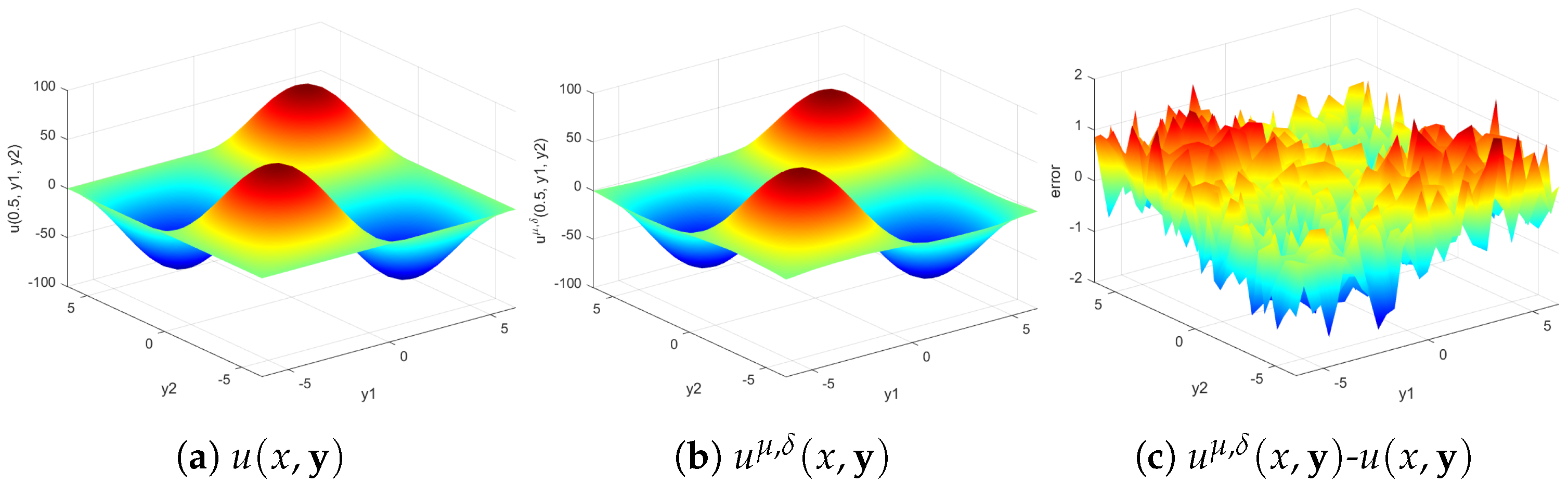
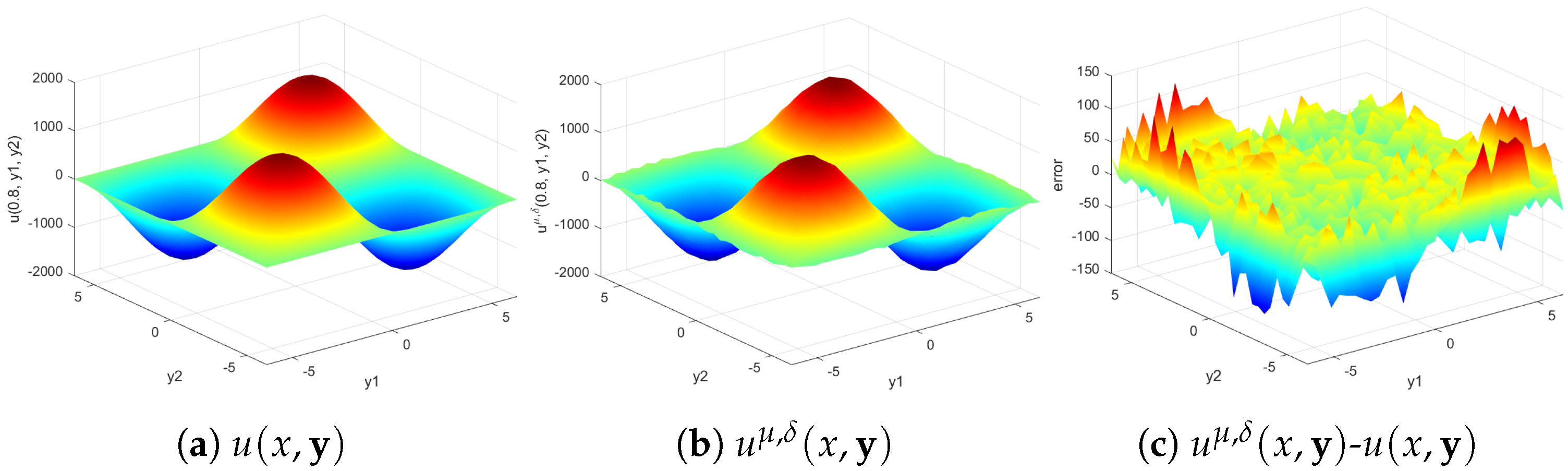
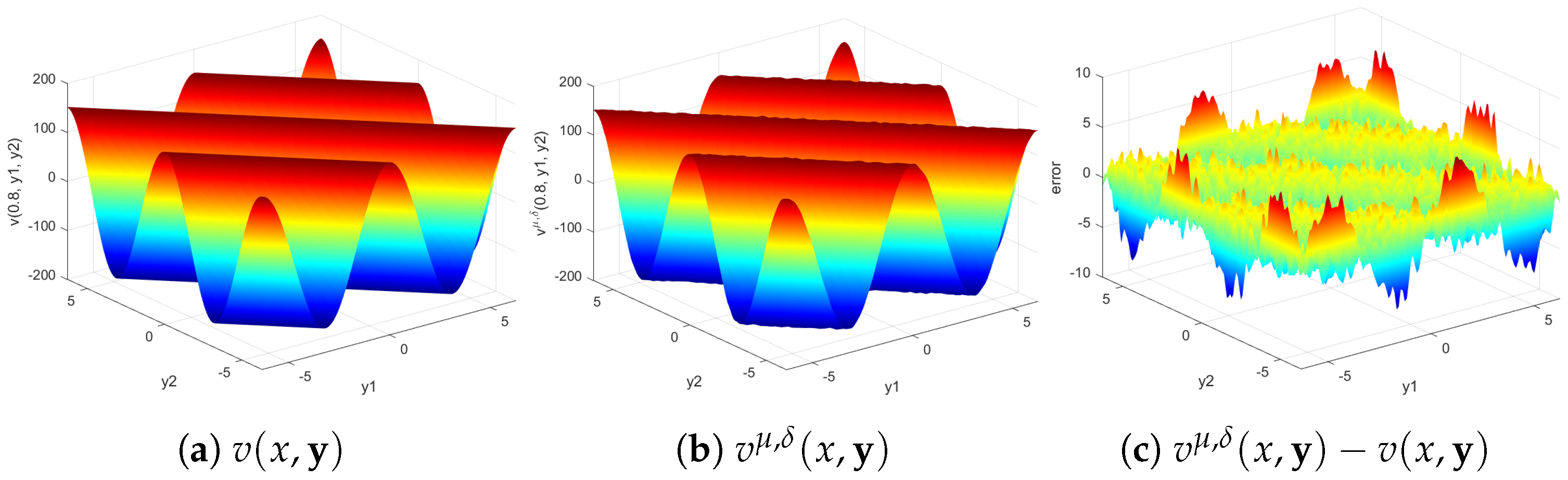
5. Numerical Experiments

In this section, we show the numerical validity of the proposed method by two numerical examples. The numerical experiments are carried out using MATLAB R2016b. The steps are as follows: first, we give the exact solution $u(x,\mathbf{y})$ or $v(x,\mathbf{y})$ and get the exact boundary data $f(\mathbf{y})=u(0,\mathbf{y})$ or $g(\mathbf{y})=v_x(0,\mathbf{y})$; second, we simulate the measured data $f^{\delta }(\mathbf{y})$ or $g^{\delta }(\mathbf{y})$ by adding random noise to $f(\mathbf{y})$ or $g(\mathbf{y})$; third, we get the regularization solution $u^{\mu ,\delta }(x,\mathbf{y})$ by (13) or $v^{\mu ,\delta }(x,\mathbf{y})$ by (14).

Considering the case of $n=2$, we set the domain of $\mathbf{y}$ as $[-2\pi ,2\pi ]\times [-2\pi ,2\pi ]$. The measured data $f(\mathbf{y})$ and $g(\mathbf{y})$ are generated by

$$\begin{array}{c}\hfill f^{\delta }=f+ϵ(2randn(size(f)-1))\end{array},$$

where

$$\begin{array}{c}\hfill f={(f_{ij})}_{n\times n}={(f(y_i,y_j))}_{n\times n},y_i=-2\pi +{\displaystyle \frac{4\pi (i-1)}{n-1}},i=1,2,\cdots ,n,\end{array}$$

and the function “$randn(·)$” generates arrays of random data with a mean of 0 and variance of ${\sigma }^2=1$. The error level is

$$\delta =\parallel f^{\delta }-f\parallel ={\displaystyle \frac{4\pi }{n}}\sqrt{\sum _{i,j=1}^n{(f_{ij}^{\delta }-f_{ij})}^2}.$$

The relative error of the regularization solution $u^{\mu ,\delta }$ is

$$\begin{array}{c}\hfill rel(u^{\mu ,\delta })={\displaystyle \frac{\parallel u^{\mu ,\delta }(x,·)-u(x,·)\parallel }{\parallel u(x,·)\parallel }}.\end{array}$$

We always take $n=129$ in the numerical experiments. The a posteriori regularization parameter $\mu =\mu (\delta )$ is determined by (13) or (14) using the bisection method.

Example 1.

Let the exact solution of (3) be

$$u(x,\mathbf{y})=u(x,y_1,y_2)=sin{\displaystyle \frac{y_1}{2}}sin{\displaystyle \frac{y_2}{2}}cosh(x\sqrt{k^2+{\displaystyle \frac{1}{2}}}),$$

where k is the wave number. Then, we have

$$f(\mathbf{y})=u(0,\mathbf{y})=sin{\displaystyle \frac{y_1}{2}}sin{\displaystyle \frac{y_2}{2}}.$$

Table 1. The relative errors of the regularization solution $rel(u^{\mu ,\delta })$ with the Gaussian kernel function at $x=0.2$ for different $ϵ$ and k.

$\mathit{ϵ}$		$0.1$	$0.01$	$0.001$	$0.0001$
$apriori$	$k=1$	$0.233680$	$0.159344$	$0.117272$	$0.070912$
	$k=10$	$0.234835$	$0.159938$	$0.117797$	$0.071367$
	$k=100$	$0.235930$	$0.160133$	$0.117868$	$0.071860$
$aposteriori$	$k=1$	$0.112525$	$0.079810$	$0.031275$	$0.017466$
	$k=10$	$0.113050$	$0.080876$	$0.032780$	$0.017826$
	$k=100$	$0.113058$	$0.080909$	$0.034385$	$0.018324$

,

Table 2. The relative errors of the regularization solution $rel(u^{\mu ,\delta })$ with the Dirichlet kernel function at $x=0.2$ for different $ϵ$ and k.

$\mathit{ϵ}$		$0.1$	$0.01$	$0.001$	$0.0001$
$apriori$	$k=1$	$0.268808$	$0.199017$	$0.129024$	$0.085737$
	$k=10$	$0.271318$	$0.199420$	$0.129214$	$0.091286$
	$k=100$	$0.273179$	$0.199462$	$0.129992$	$0.091387$
$aposteriori$	$k=1$	$0.123046$	$0.085015$	$0.059284$	$0.024477$
	$k=10$	$0.127065$	$0.085118$	$0.059289$	$0.022827$
	$k=100$	$0.127246$	$0.085211$	$0.059296$	$0.022905$

and

Table 3. The relative errors of the regularization solution $rel(u^{\mu ,\delta })$ with the Poussin kernel function at $x=0.2$ for different $ϵ$ and k.

$\mathit{ϵ}$		$0.1$	$0.01$	$0.001$	$0.0001$
$apriori$	$k=1$	$0.259040$	$0.183093$	$0.125741$	$0.085630$
	$k=10$	$0.272195$	$0.183271$	$0.125906$	$0.087056$
	$k=100$	$0.281887$	$0.184352$	$0.126475$	$0.087284$
$aposteriori$	$k=1$	$0.113688$	$0.083249$	$0.039925$	$0.019824$
	$k=10$	$0.117872$	$0.083636$	$0.041173$	$0.022638$
	$k=100$	$0.119315$	$0.083901$	$0.042274$	$0.022715$

show the relative errors of the regularization solution $rel(u^{\mu ,\delta })$ at $x=0.2$ for different $ϵ$ and k when the regularization parameter is chosen by the a priori and a posteriori strategies. We take the regularization convolution kernel function $\widehat{P}(\xi )$ as the Gaussian kernel, the Dirichlet kernel, and the Poussin kernel function, respectively.

Table 1, Table 2 and Table 3 show the following four facts:

(1)

The regularization solution $u^{\mu ,\delta }(x,\mathbf{y})$ is stable for both the a priori and a posteriori parameter choice strategy;

(2)

The results of the regularization solution $u^{\mu ,\delta }(x,\mathbf{y})$ are still well for high wave number k;

(3)

The results of the a posteriori choice strategy are better than those of the a priori choice strategy;

(4)

The Gaussian kernel function has a slight advantage over the other two kernel functions.

Therefore, the a posteriori parameter choice strategy and the Gaussian kernel function are used in the following experiments. When $ϵ=0.01$ and $k=100$, the exact solution $u(x,\mathbf{y})$, the regularization solution $u^{\mu ,\delta }(x,\mathbf{y})$, and the error $u^{\mu ,\delta }(x,\mathbf{y})-u(x,\mathbf{y})$ at $x=0.2$, $x=0.5$, and $x=0.8$ are given in Figure 1, Figure 2 and Figure 3, respectively. Figure 1, Figure 2 and Figure 3 show that the regularization solution $u^{\mu ,\delta }(x,\mathbf{y})$ can approximate the exact solution $u(x,\mathbf{y})$ well, and the approximation effect of $u^{\mu ,\delta }(x,\mathbf{y})$ is better for smaller x.

Example 2.

Let the exact solution of (4) be

$$v(x,\mathbf{y})=v(x,y_1,y_2)=cos(y_1+y_2){\displaystyle \frac{sinh(x\sqrt{k^2+1/2})}{\sqrt{k^2+1/2}}},$$

where k is the wave number. Then, we have

$$g(\mathbf{y})=v_x(0,\mathbf{y})=cos(y_1+y_2).$$

Table 4. The relative errors of the regularization solution $rel(v^{\mu ,\delta })$ with the Gaussian kernel function at $x=0.2$ for different $ϵ$ and k.

$\mathit{ϵ}$		$0.1$	$0.01$	$0.001$	$0.0001$
$apriori$	$k=1$	$0.346058$	$0.080304$	$0.042824$	$0.033628$
	$k=10$	$0.349183$	$0.082115$	$0.044944$	$0.035809$
	$k=100$	$0.351843$	$0.088390$	$0.052139$	$0.043055$
$aposteriori$	$k=1$	$0.117750$	$0.068838$	$0.035348$	$0.011900$
	$k=10$	$0.120404$	$0.071982$	$0.036363$	$0.013695$
	$k=100$	$0.126416$	$0.077805$	$0.044492$	$0.017960$

,

Table 5. The relative errors of the regularization solution $rel(v^{\mu ,\delta })$ with the Dirichlet kernel function at $x=0.2$ for different $ϵ$ and k.

$\mathit{ϵ}$		$0.1$	$0.01$	$0.001$	$0.0001$
$apriori$	$k=1$	$0.855277$	$0.128594$	$0.086578$	$0.071735$
	$k=10$	$0.855221$	$0.129458$	$0.085031$	$0.071980$
	$k=100$	$0.855772$	$0.129776$	$0.086976$	$0.072002$
$aposteriori$	$k=1$	$0.124472$	$0.086636$	$0.055169$	$0.017641$
	$k=10$	$0.127957$	$0.084905$	$0.061391$	$0.022857$
	$k=100$	$0.129509$	$0.088039$	$0.063265$	$0.025268$

and

Table 6. The relative errors of the regularization solution $rel(v^{\mu ,\delta })$ with the Poussin kernel function at $x=0.2$ for different $ϵ$ and k.

$\mathit{ϵ}$		$0.1$	$0.01$	$0.001$	$0.0001$
$apriori$	$k=1$	$0.741338$	$0.124538$	$0.052405$	$0.047151$
	$k=10$	$0.744302$	$0.126333$	$0.052473$	$0.047907$
	$k=100$	$0.744574$	$0.127423$	$0.052592$	$0.048278$
$aposteriori$	$k=1$	$0.123952$	$0.084619$	$0.051950$	$0.017559$
	$k=10$	$0.126644$	$0.086460$	$0.053411$	$0.018083$
	$k=100$	$0.129783$	$0.090114$	$0.059655$	$0.022334$

show the relative errors of the regularization solution $rel(v^{\mu ,\delta })$ at $x=0.2$ for different $ϵ$ and k. We take the regularization convolution kernel function ${\widehat{P}}_{\mu }(\xi )$ as the Gaussian kernel, the Dirichlet kernel, and the Poussin kernel function, respectively.

The results given in Table 4, Table 5 and Table 6 are similar to those of Table 1, Table 2 and Table 3; therefore, the a posteriori parameter choice strategy and the Gaussian kernel function are used next. When $ϵ=0.01$ and $k=100$, the exact solution $v(x,\mathbf{y})$, the regularization solution $v^{\mu ,\delta }(x,\mathbf{y})$, and the error $v^{\mu ,\delta }(x,\mathbf{y})-v(x,\mathbf{y})$ at $x=0.2$, $x=0.5$, and $x=0.8$ are given in Figure 4, Figure 5 and Figure 6, respectively. The results are similar to those of Example 1.

6. Discussion

Numerical experiments show that the regularization solution is stable for both the a priori and a posteriori parameter choice strategies. Compared with the a priori choice strategy, the results of the a posteriori choice strategy are better. The numerical results show that the Gaussian kernel function is superior to the Dirichlet and the Poussin kernel function. The graphs given in Examples 1 and 2 show that the approximation effect of the regularization solution is better for smaller $x\in (0,1)$.

7. Conclusions

In this paper, we propose a general framework of the mollification regularization method to solve the Cauchy problem for a multi-dimensional modified Helmholtz equation. The common conditions that the regularization convolution kernel function should satisfy are summarized. Many kernel functions satisfy these conditions, such as the Dirichlet kernel, the Poussion kernel, the Gaussian kernel, and so on. Considering the a priori choice strategy of the regularization parameter, we give the convergence rate of the regularization solution when $0<x<1$ and $x=1$, respectively. A new a posteriori choice strategy of the regularization parameter based on Morozov’s discrepancy principle is introduced, and the convergence rate of the regularization solution is also given when $0<x<1$. Numerical experiments show that the a posteriori parameter choice strategy is better than the a priori strategy, and the Gaussian kernel function has a slight advantage over the other kernel functions.

For future research, we plan to continue our research on the a posteriori choice strategy of the regularization parameter and apply the general mollification regularization method to solve other ill-posed problems, e.g., the inverse heat conduction problem, the edge detection problem, the inverse source problem of diffusion equations, etc.

References

1. Nguyen, H.T.; Tran, Q.V.; Nguyen, V.T. Some remarks on a modified Helmholtz equation with inhomogeneous source. Appl. Math. Model. 2013, 37, 793–814. [Google Scholar] [CrossRef]
2. Cheng, H.W.; Huang, J.F.; Leiterman, T.J. An adaptive fast solver for the modified Helmholtz equation in two dimensions. J. Comput. Phys. 2006, 211, 616–637. [Google Scholar] [CrossRef]
3. Manoussakis, G. A new modified Helmholtz equation for the expression of the gravity gradient and the intensity of an electrostatic field in spherical harmonics. Mathematics 2023, 11, 4326. [Google Scholar] [CrossRef]
4. Reginska, T.; Reginski, K. Approximate solution of a Cauchy problem for the Helmholtz equation. Inverse Probl. 2006, 22, 975–989. [Google Scholar] [CrossRef]
5. Xiong, X.T.; Shi, W.X.; Fan, X.Y. Two numerical methods for a Cauchy problem for modified Helmholtz equation. Appl. Math. Model. 2011, 35, 4951–4964. [Google Scholar] [CrossRef]
6. Marin, L.; Elliott, L.; Heggs, P.J.; Ingham, D.B.; Lesnic, D.; Wen, X. Conjugate gradient-boundary element solution to the Cauchy problem for Helmholtz-type equations. Comput. Mech. 2003, 31, 367–377. [Google Scholar] [CrossRef]
7. Qin, H.H.; Wei, T. Quasi-reversibility and truncation methods to solve a Cauchy problem of the modified Helmholtz equation. Math. Comput. Simulat. 2009, 80, 352–366. [Google Scholar] [CrossRef]
8. Cheng, H.; Zhu, P.; Gao, J. A regularization method for the cauchy problem of the modified Helmholtz equation. Math. Meth. Appl. Sci. 2015, 38, 3711–3719. [Google Scholar] [CrossRef]
9. Chen, Y.G.; Yang, F.; Ding, Q. The Landweber iterative regularization method for solving the Cauchy problem of the modified Helmholtz equation. Symmetry 2022, 14, 1209. [Google Scholar] [CrossRef]
10. Fu, C.L.; Feng, X.L.; Qian, Z. The Fourier regularization for solving the Cauchy problem for the Helmholtz equation. Appl. Numer. Math. 2009, 59, 2625–2640. [Google Scholar] [CrossRef]
11. He, S.Q.; Feng, X.F. A regularization method to solve a Cauchy problem for the two-dimensional modified Helmholtz equation. Mathematics 2019, 7, 360. [Google Scholar] [CrossRef]
12. Jday, F.; Omri, H. Adaptive Runge-Kutta regularization for a Cauchy problem of a modified Helmholtz equation. J. Inverse Ill-Posed Probl. 2023, 31, 351–374. [Google Scholar] [CrossRef]
13. Hao, D.N. A mollification method for ill-posed problems. Numer. Math. 1994, 68, 469–506. [Google Scholar]
14. Murio, D.A. The Mollification Method and the Numerical Solution of Ill-Posed Problems; Wiley-Interscience Publication: New York, NY, USA, 1993. [Google Scholar]
15. Basu, M. Gaussian-based edge-detection methods—A survey. IEEE Trans Syst. Man Cybern. C 2002, 32, 252–260. [Google Scholar] [CrossRef]
16. Yang, F.; Fu, C.L. A mollification regularization method for the inverse spatial-dependent heat source problem. J. Comput. Appl. Math. 2014, 255, 555–567. [Google Scholar] [CrossRef]
17. He, S.Q.; Feng, X.F. A mollification regularization method with the Dirichlet Kernel for two Cauchy problems of three-dimensional Helmholtz equation. Int. J. Comput. Math. 2020, 97, 2320–2336. [Google Scholar] [CrossRef]
18. Fu, C.L.; Ma, Y.J.; Zhang, Y.X.; Yang, F. A a posteriori regularization for the Cauchy problem for the Helmholtz equation with inhomogeneous Neumann data. Appl. Math. Model. 2015, 39, 4103–4120. [Google Scholar] [CrossRef]
19. He, S.Q.; Di, C.N.; Yang, L. The mollification method based on a modified operator to the ill-posed problem for 3D Helmholtz equation with mixed boundary. Appl. Numer. Math. 2021, 160, 422–435. [Google Scholar] [CrossRef]
20. Li, Z.P.; Xu, C.; Lan, M.; Qian, Z. A mollification method for a Cauchy problem for the Helmholtz equation. Int. J. Comput. Math. 2018, 95, 2256–2268. [Google Scholar] [CrossRef]
21. Kirsch, A. An Introduction to the Mathematical Theory of Inverse Problems, 2nd ed.; Springer: New York, NY, USA, 2011. [Google Scholar]
Figure 1. The exact solution u ( x , y ) , the regularization solution u μ , δ ( x , y ) , and the absolute value of the error u μ , δ ( x , y ) u ( x , y ) at x = 0.2 when ϵ = 0.01 and k = 100 .
Symmetry 16 01549 g001
Figure 2. The exact solution u ( x , y ) , the regularization solution u μ , δ ( x , y ) , and the error u μ , δ ( x , y ) u ( x , y ) at x = 0.5 when ϵ = 0.01 and k = 100 .
Symmetry 16 01549 g002
Figure 3. The exact solution u ( x , y ) , the regularization solution u μ , δ ( x , y ) , and the error u μ , δ ( x , y ) u ( x , y ) at x = 0.8 when ϵ = 0.01 and k = 100 .
Symmetry 16 01549 g003
Figure 4. The exact solution v ( x , y ) , the regularization solution v μ , δ ( x , y ) , and the error v μ , δ ( x , y ) v ( x , y ) at x = 0.2 when ϵ = 0.01 and k = 100 .
Symmetry 16 01549 g004
Figure 5. The exact solution v ( x , y ) , the regularization solution v μ , δ ( x , y ) , and the error v μ , δ ( x , y ) v ( x , y ) at x = 0.5 when ϵ = 0.01 and k = 100 .
Symmetry 16 01549 g005
Figure 6. The exact solution v ( x , y ) , the regularization solution v μ , δ ( x , y ) , and the error v μ , δ ( x , y ) v ( x , y ) at x = 0.8 when ϵ = 0.01 and k = 100 .
Symmetry 16 01549 g006