Gain-Scheduled Energy-to-Peak Approach for Vehicle Sideslip Angle Filtering

Abstract

The ongoing development of gain-scheduled filters is motivated by the estimation of the sideslip angle of ground vehicles. The present work proposes an approach based on finite-frequency specifications and an energy-to-peak (E2P) index for designing linear parameter-varying (LPV) filters. After reporting a new theoretical result, analysis and synthesis conditions are proposed for gain-scheduled and robust filters. Their properties are tested and illustrated using a simulated ground vehicle system via a comparative study, highlighting the advantages of the proposed approach.

1. Introduction

In emergency circumstances, the stability of vehicles depends on the control system receiving accurate information on the sideslip angle and yaw rate [1,2]. In particular, while sideslip angle estimation is critical, it is not currently measurable using an affordable physical sensor [3]. To address this, researchers are proposing algorithms to estimate the sideslip angle from other physical sensor-based measurements. For instance, Ref. [4] has proposed a sideslip angle estimation method for autonomous vehicles, whereas in [5], an $H_{\infty }$ estimator for the sideslip angle of an electric ground vehicle was investigated via finite-frequency (FF) specification using a polytopic solution set. Recently, Ref. [6] studied the robust $H_{\infty }$ filter design issue via a Takagi–Sugeno model with sensor failure using data dropouts and dynamic quantization.

It is worth mentioning that the vehicle wheel steering angle, which is the main input to the LPV lateral dynamics model, operates in the low-frequency domain. Thus, filters designed taking minimization in the entire-frequency EF (full-frequency) domain into account may not be adequate in practice. Therefore, the use of finite-frequency methodologies, such as FF $H_{\infty }$ filtering, has been explored in various contexts, including polytopic systems [7] and Takagi–Sugeno (TS) fuzzy systems [8] via the generalized Kalman–Yakubovic–Popov lemma [9]. The methodologies discussed here are specifically designed to mitigate the inherent conservatism linked to the incorporation of weighting matrices. These approaches have been applied to various problem domains, notably in the context of $H_{\infty }$ gain-scheduled control for continuous linear parameter-varying (LPV) systems, as elucidated in the context of FF domains in [3,10].

However, when the filtering error is limited in magnitude, the energy-to-peak (E2P) filtering, also known as generalized $H_2$ filtering [11] or $L_2-L_{\infty }$ filtering, has been shown to be the most adequate solution [12]. In this context, Ref. [13] developed E2P performance for continuous-time systems, focusing on minimizing the peak value of the estimation error for all potential disturbances with bounded energy [11]. In the case of vehicle system design, several works [14] have focused on resilient E2P filter design, where E2P estimations are frequently used as a measure of performance; see, for example, Ref. [15], in which E2P was used to design controllers that improved lateral dynamics, or the recent publication [16] that demonstrated the importance of E2P for mitigation of disturbances in car suspension systems. Despite these works, E2P approaches in the context of sideslip angle are not well-studied and are limited to [17], where the E2P Luenberger observer has been proposed. On the other hand, gain-scheduled systems-based approaches have been demonstrating good performance in vehicles; see, for instance, Refs. [15,18] for controller design and [19] for filter design. Nevertheless, except for T–S fuzzy systems, in which the unknown membership method is applied [20], an E2P gain-scheduled FF filter design for linear parameter-varying (LPV) systems has not been studied, motivating the research presented in this paper.

Gain-scheduled energy-to-peak (E2P) filtering for ground vehicle sideslip angle estimation was investigated in this study. Our objective was to determine the E2P FF conditions under which the desired filter exists and the filtering error system satisfies the specified E2P performance index. The aim of the proposed approach is to minimize the energy-to-peak value, as this measure of performance [21] has been demonstrated to be the most adequate in related practical problems. As an example, Ref. [22] has successfully demonstrated this method’s application to a data transmission problem. Based on Finsler’s lemma, free-weighting matrices (slacks) are introduced to generate additional free dimensions in the solution space. The result is more general than the previous results in the literature and contains norm-bounded uncertainty conditions. Finsler’s lemma was selected to solve this problem, as it has repeatedly been shown to be useful in deriving novel stability results that are computationally feasible in practical problems; see, for example, Ref. [23], in which the lemma was applied to data-driven control design, including when the noisy data, and [24], in which it was applied to a fault-detection problem of electrical systems. A gain-scheduled FF filter parameter design is proposed using a suitable form of the introduced free-weighting matrices, which leads to a new filter design with fewer conservative conditions. The simulation section demonstrates the proposed approach for estimating the sideslip angle of ground vehicles. Finally, a comparison is made to show the superiority of the proposed approach when compared with others. It is pointed out that the results in this paper were validated via simulations, as vehicle dynamics simulations have been extensively validated (see, for instance, Refs. [25,26] and references therein) and shown to reduce costs and development times for new designs and technologies [26].

To summarize, the main contributions of this study are as follows:

• The sideslip angle filtering problem is solved using a novel approach.
• New results for energy-to-peak optimization of LPV systems are provided, focusing on low frequencies.
• These results include new stability conditions for LPV systems in low frequencies.

Notation: The identity matrix of dimension s is denoted by $I_s$. Positive (negative) definite matrices are denoted by $P>0$ $(P<0)$. ∗ is a symmetric term of a square symmetric matrix. The null space of $\vartheta$ is ${\vartheta }^{\perp }$ (i.e., $\vartheta$ ${\vartheta }^{\perp }$ = 0). For a matrix R, $Tr\left(R\right)$ is its trace, $R^T$ its conjugate transpose and $\mathrm{Sym}\left(R\right)=R+R^T$. Time-varying elements $\rho \left(t\right)$ are shortened to ${\rho }_t$.

2. Problem Statement and Preliminaries

2.1. Lateral Dynamics Model

Vehicle dynamics have been extensively studied in the literature in order to develop mathematical models (see, for instance, Refs. [27,28] and references therein). To simplify the presentation of the results, the lateral dynamics of the vehicle are condensed here as a two-degree-of-freedom model following Figure 1. A mathematical model is then proposed, which is simplified as much as possible with the objective of presenting the general methodology in a clear way. It is pointed out that the approach presented may be applied to more detailed models, such as those in [27] and references therein.

The notation considered for the lateral dynamics is schematized in Figure 1: the vehicle’s overall mass is denoted by m; $I_z$ represents its moment of inertia around the yaw axis, passing through the center of gravity (CG); and the front axis is positioned $l_f$ distance away from the CG, while the rear axis is positioned $l_r$ distance away from it. It is assumed that $V=[v_x,v_y]$ is the vector of vehicle speed, where $v_x$ and $v_y$ are the longitudinal and lateral speeds, respectively. The variables and nominal parameters of the model are listed in

Table 1. Main vehicle variables with nominal values used for the validation.

Symbol	Variable	Units
$\varpi \left(t\right)$	Yaw rate	rad/s
$\beta \left(t\right)$	Sideslip angle	rad
$\theta \left(t\right)$	Wheel steering angle	rad
$m$	Vehicle mass	880 Kg
$I_z$	Yaw inertia moment	728 Kg.m2
$c_r$	Rear-wheel cornering stiffness	15,000 N/rad
$c_f$	Front-wheel cornering stiffness	15,000 N/rad
$l_f$	Distance from front axis to $\mathrm{CG}$	0.808 m
$l_r$	Distance from rear axis to $\mathrm{CG}$	1.082 m

.

The following tire cornering stiffness model in [17] with uncertainties is used since the relationship between the lateral force and the wheel slip angle are complex due to non-linearities in the lateral tire model:

$$\left\{\begin{array}{c}\left(c_f+\Delta c_f{\mathbb{R}}_t\right)={\widehat{c}}_f,\hfill \\ \left(c_r+\Delta c_r{\mathbb{R}}_t\right)={\widehat{c}}_r,\hfill \end{array}\right.$$

(1)

where the tire cornering stiffness values are ${\widehat{c}}_r$ and ${\widehat{c}}_f$, with their nominal values being $c_r$ and $c_f$, respectively. $|{\mathbb{R}}_t|\le 1$ condenses the uncertainty, with bounds $\Delta c_r$ and $\Delta c_f$, which are determined in advance.

Considering that the longitudinal velocity fluctuates within the range of ${\underline{v}}_x$ and ${\overline{v}}_x$, and utilizing the aforementioned symbols to denote the sideslip angle and yaw motion of the vehicle, the filtering methodology employed in this investigation is rooted in the lateral dynamics of the vehicle. This consideration implies that the lateral dynamics of the vehicle model can be cast as an LPV system. Our challenge is how to deal with the conservatism and the computational load. For this purpose, the velocity $v_x$ is assumed to belong to $[{\underline{v}}_x,{\overline{v}}_x]$, with $0<{\underline{v}}_x<{\overline{v}}_x$ known bounds. Then, ${\displaystyle \frac{1}{v_x}}$ varies within the range $[{\displaystyle \frac{1}{{\overline{v}}_x}},{\displaystyle \frac{1}{{\underline{v}}_x}}]$, and the variable ${\displaystyle \frac{1}{v_x^2}}$ is within the range $[{\displaystyle \frac{1}{{\overline{v}}_x^2}},{\displaystyle \frac{1}{{\underline{v}}_x^2}}]$. However, as the varying parameters are velocity-related—that is, they are not independently variant—some methods are proposed to shrink the polytope to reduce the condition conservatism. A straightforward method is to employ a rectangular polytope to cover all the possible choices for the parameter pair $({\displaystyle \frac{1}{v}},{\displaystyle \frac{1}{v^2}})$. However, the method would increase the conservatism as the rectangular polytope would cover many unreachable areas. To address this, a triangular polytope is used in the current work to describe the parameter pair, following [3,17].

Following the modeling in [5], the two-degree-of-freedom model above may be represented as the following LPV state-space model:

$$\left\{\begin{array}{c}{\dot{\chi }}_t=\mathbb{A}\left({\delta }_t\right){\chi }_t+\mathbb{B}\left({\delta }_t\right){\theta }_t,\hfill \\ {\mathrm{y}}_t=\mathbb{C}{\chi }_t,\hfill \\ {\mathrm{z}}_t=\mathbb{L}{\chi }_t.\hfill \end{array}\right.$$

(2)

where ${\chi }_t={\left[\begin{array}{cc}{\beta }^T\hfill & {\varpi }^T\hfill \end{array}\right]}^T\in {\Re }^n$ is the state; ${\mathrm{z}}_t\in {\Re }^q$ is the output to be estimated, ${\mathrm{y}}_t\in {\Re }^p$ is the measured output; and ${\theta }_t\in {\Re }^m$ is the wheel steering angle, considered as a bounded perturbation in ${\mathcal{L}}_2$$[0,+\infty )$. It is assumed that the system matrices (parameter dependents and constants) are given by

$$\begin{array}{cc}& \mathbb{A}\left({\delta }_t\right)=\overline{\mathbb{A}}\left({\delta }_t\right)+{\mathbb{F}}_{\mathbb{A}}\left({\delta }_t\right){\mathbb{M}}_t{\mathbb{E}}_{\mathbb{A}}=\sum _{i=1}^3{\delta }_i\left({\overline{\mathbb{A}}}_i+{\mathbb{F}}_{\mathbb{A}i}{\mathbb{M}}_t{\mathbb{E}}_{\mathbb{A}}\right),{\mathbb{M}}_t=\left[\begin{array}{cc}{\mathbb{R}}_t& 0\\ 0& {\mathbb{R}}_t\end{array}\right]\hfill \\ & \mathbb{B}\left({\delta }_t\right)=\overline{\mathbb{B}}\left({\delta }_t\right)+{\mathbb{F}}_{\mathbb{B}}\left({\delta }_t\right){\mathbb{M}}_t{\mathbb{E}}_{\mathbb{B}}=\sum _{i=1}^3{\delta }_i\left({\overline{\mathbb{B}}}_i+{\mathbb{F}}_{\mathbb{B}i}{\mathbb{M}}_t{\mathbb{E}}_{\mathbb{B}}\right),{\mathbb{E}}_{\mathbb{A}}=I,{\mathbb{E}}_{\mathbb{B}}=\left[\begin{array}{c}1\hfill \\ 1\hfill \end{array}\right]\hfill \end{array}$$

$$\begin{array}{cc}& {\overline{\mathbb{A}}}_1=\left[\begin{array}{cc}{\displaystyle \frac{-c_f-c_r}{m{\overline{v}}_x}}& {\displaystyle \frac{l_r{c}_r-l_f{c}_f}{m{\overline{v}}_x^2}}-1\\ {\displaystyle \frac{l_r{c}_r-l_f{c}_f}{I_z}}& {\displaystyle \frac{-l_f^2{c}_f-l_r^2{c}_r}{I_z{\overline{v}}_x}}\end{array}\right],{\overline{\mathbb{A}}}_2=\left[\begin{array}{cc}{\displaystyle \frac{-c_f-c_r}{m}}\times {\displaystyle \frac{{\overline{v}}_x+{\underline{v}}_x}{2{\overline{v}}_x{\underline{v}}_x}}& {\displaystyle \frac{l_r{c}_r-l_f{c}_f}{m{\overline{v}}_x{\underline{v}}_x}}-1\\ {\displaystyle \frac{l_r{c}_r-l_f{c}_f}{I_z}}& {\displaystyle \frac{-l_f^2{c}_f-l_r^2{c}_r}{I_z}}\times {\displaystyle \frac{{\overline{v}}_x+{\underline{v}}_x}{2{\overline{v}}_x{\underline{v}}_x}}\end{array}\right],\hfill \\ & {\overline{\mathbb{A}}}_3=\left[\begin{array}{cc}{\displaystyle \frac{-c_f-c_r}{m{\underline{v}}_x}}& {\displaystyle \frac{l_r{c}_r-l_f{c}_f}{m{\underline{v}}_x^2}}-1\\ {\displaystyle \frac{l_r{c}_r-l_f{c}_f}{I_z}}& {\displaystyle \frac{-l_f^2{c}_f-l_r^2{c}_r}{I_z{\underline{v}}_x}}\end{array}\right]{\overline{\mathbb{B}}}_1=\left[\begin{array}{c}{\displaystyle \frac{c_f}{m{\overline{v}}_x}}\\ {\displaystyle \frac{l_f{c}_f}{I_z}}\end{array}\right],{\overline{\mathbb{B}}}_2=\left[\begin{array}{c}{\displaystyle \frac{c_f}{m}}\times {\displaystyle \frac{{\overline{v}}_x+{\underline{v}}_x}{2{\overline{v}}_x{\underline{v}}_x}}\\ {\displaystyle \frac{l_f{c}_f}{I_z}}\end{array}\right],{\overline{\mathbb{B}}}_3=\left[\begin{array}{c}{\displaystyle \frac{c_f}{m{\underline{v}}_x}}\\ {\displaystyle \frac{l_f{c}_f}{I_z}}\end{array}\right]\hfill \end{array}$$

$$\begin{array}{cc}& \mathbb{L}=\left[\begin{array}{cc}1\hfill & 0\hfill \end{array}\right],\mathbb{C}=\left[\begin{array}{cc}0\hfill & 1\hfill \end{array}\right]\hfill \end{array}$$

$$\begin{array}{cc}& {\mathbb{F}}_{\mathbb{A}1}=\left[\begin{array}{cc}{\displaystyle \frac{-\Delta c_f-\Delta c_r}{m{\overline{v}}_x}}& {\displaystyle \frac{l_r\Delta c_r-l_f\Delta c_f}{m{\overline{v}}_x^2}}\\ {\displaystyle \frac{l_r\Delta c_r-l_f\Delta c_f}{I_z}}& {\displaystyle \frac{-l_f^2\Delta c_f-l_r^2\Delta c_r}{I_z{\overline{v}}_x}}\end{array}\right],{\mathbb{F}}_{\mathbb{A}2}=\left[\begin{array}{cc}{\displaystyle \frac{-\Delta c_f-\Delta c_r}{m}}\times {\displaystyle \frac{{\overline{v}}_x+{\underline{v}}_x}{2{\overline{v}}_x{\underline{v}}_x}}& {\displaystyle \frac{l_r\Delta c_r-l_f\Delta c_f}{m{\overline{v}}_x{\underline{v}}_x}}\\ {\displaystyle \frac{l_r\Delta c_r-l_f\Delta c_f}{I_z}}& {\displaystyle \frac{-l_f^2\Delta c_f-l_r^2\Delta c_r}{I_z}}\times {\displaystyle \frac{{\overline{v}}_x+{\underline{v}}_x}{2{\overline{v}}_x{\underline{v}}_x}}\end{array}\right],\hfill \\ & {\mathbb{F}}_{\mathbb{A}3}=\left[\begin{array}{cc}{\displaystyle \frac{-\Delta c_f-\Delta c_r}{m{\underline{v}}_x}}& {\displaystyle \frac{l_r\Delta c_r-l_f\Delta c_f}{m{\underline{v}}_x^2}}\\ {\displaystyle \frac{l_r\Delta c_r-l_f\Delta c_f}{I_z}}& {\displaystyle \frac{-l_f^2\Delta c_f-l_r^2\Delta c_r}{I_z{\underline{v}}_x}}\end{array}\right],{\mathbb{F}}_{\mathbb{B}1}=\left[\begin{array}{cc}{\displaystyle \frac{\Delta c_f}{m{\overline{v}}_x}}& 0\\ 0& {\displaystyle \frac{l_f\Delta c_f}{I_z}}\end{array}\right],\hfill \\ & {\mathbb{F}}_{\mathbb{B}2}=\left[\begin{array}{cc}{\displaystyle \frac{\Delta c_f}{m}}\times {\displaystyle \frac{{\overline{v}}_x+{\underline{v}}_x}{2{\overline{v}}_x{\underline{v}}_x}}& 0\\ 0& {\displaystyle \frac{l_f\Delta c_f}{I_z}}\end{array}\right],{\mathbb{F}}_{\mathbb{B}3}=\left[\begin{array}{cc}{\displaystyle \frac{\Delta c_f}{m{\underline{v}}_x}}& 0\\ 0& {\displaystyle \frac{-l_f\Delta c_f}{I_z}}\end{array}\right].\hfill \end{array}$$

Moreover, let us define ${\delta }_t$ as a time-varying parameter vector of dimension S, representing the LPV parameter and belonging to a simplex unit:

$$\Omega =\{\beta \in {\Re }^S:\sum _{i=1}^S{\beta }_i=1;{\beta }_i\ge 0,i=1,\dots ,S\}$$

(3)

These parameters are bounded by known rates of variations: $|\dot{{\delta }_i}|\le {\overline{\delta }}_i$, $(i=1,\dots ,S)$. Then, we can build a convex set (polytope) to which $\dot{{\delta }_i}$ belongs [29], described by the following:

$${\Omega }_d=\{\dot{\delta }\in {\Re }^S:\sum _{i=1}^S\dot{{\delta }_i}=0;|\dot{{\delta }_i}|\le {\overline{\delta }}_i,i=1,\dots ,S\}$$

(4)

Consequently, the system matrices with compatible dimensions can be represented by the following:

$$\left[\begin{array}{cc}\mathbb{A}\left({\delta }_t\right)& \mathbb{B}\left({\delta }_t\right)\end{array}\right]=\sum _{i=1}^S{\delta }_{i_t}\left[\begin{array}{cc}{\mathbb{A}}_i& {\mathbb{B}}_i\end{array}\right],{\delta }_t\in \Omega .\mathrm{with} S=3$$

(5)

The assumptions used to derive this model are now summarized:

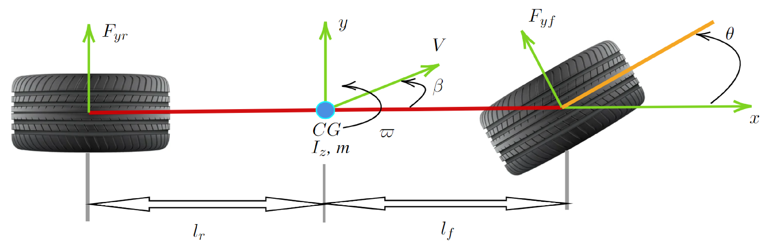
• The lateral dynamics of the vehicle correspond to the two-degree-of-freedom system presented in Figure 1.
• The two-degree-of-freedom lateral dynamics can be represented by the LPV model in Equation (2).
• The tire cornering stiffness may be represented by the model in Equation (1), with uncertain parameters.

2.2. Objectives of the Filter

The goal of the proposed filter is to estimate the value of the sideslip angle, considering that the yaw rate is measured. The dynamics of the proposed filter are as follows:

$$\left\{\begin{array}{c}{\dot{\widehat{\chi }}}_t={\mathbb{A}}_f\left({\delta }_t\right){\widehat{\chi }}_t+{\mathbb{B}}_f\left({\delta }_t\right){\mathrm{y}}_t\hfill \\ {\widehat{\mathrm{z}}}_t={\mathbb{C}}_f\left({\delta }_t\right){\widehat{\chi }}_t\hfill \end{array}\right.$$

(6)

where ${\widehat{\chi }}_t\in {\Re }^{n_f}$ is the filter state (full-order filter $n_f$ = n); ${\widehat{\mathrm{z}}}_t\in {\Re }^q$ is the estimate of ${\mathrm{z}}_t$; and ${\mathbb{A}}_f\left({\delta }_t\right)$, ${\mathbb{B}}_f\left({\delta }_t\right)$ and ${\mathbb{C}}_f\left({\delta }_t\right)$ are matrices of appropriate dimensions, which are obtained in the design section.

Next, the estimation error is defined to be ${\zeta }_t={\mathrm{z}}_t-{\widehat{\mathrm{z}}}_t$, so the augmented filtering system is as follows:

$$\left\{\begin{array}{c}{\dot{\eta }}_t={\mathbb{A}}_e\left({\delta }_t\right){\eta }_t+{\mathbb{B}}_e\left({\delta }_t\right){\theta }_t\hfill \\ {\zeta }_t={\mathbb{C}}_e\left({\delta }_t\right){\eta }_t\hfill \end{array}\right.$$

(7)

such that ${\eta }_t={\left[{\chi }_t^T{\widehat{\chi }}_t^T\right]}^T$, and the corresponding matrices are as follows:

$${\mathbb{A}}_e\left({\delta }_t\right)={\tilde{\mathbb{A}}}_e\left({\delta }_t\right)+{\mathbb{A}}_{\Delta e}\left({\delta }_t\right),{\mathbb{B}}_e\left({\delta }_t\right)={\tilde{\mathbb{B}}}_e\left({\delta }_t\right)+{\mathbb{B}}_{\Delta e}\left({\delta }_t\right),\mathrm{and}{\mathbb{C}}_e\left({\delta }_t\right)=\left[\begin{array}{cc}\mathbb{L}\left({\delta }_t\right)& -{\mathbb{C}}_f\left({\delta }_t\right)\end{array}\right],$$

with:

$${\tilde{\mathbb{A}}}_e\left({\delta }_t\right)=\left[\begin{array}{cc}\overline{\mathbb{A}}\left({\delta }_t\right)& 0\\ {\mathbb{B}}_f\left({\delta }_t\right)\mathbb{C}& {\mathbb{A}}_f\left({\delta }_t\right)\end{array}\right],{\mathbb{A}}_{\Delta e}\left({\delta }_t\right)=\left[\begin{array}{c}{\mathbb{F}}_{\mathbb{A}}\left({\delta }_t\right)\\ 0\end{array}\right]{\mathbb{M}}_t\left[{\mathbb{E}}_{\mathbb{A}}0\right]={\overline{\mathbb{F}}}_{\mathbb{A}}\left({\delta }_t\right){\mathbb{M}}_t{\overline{\mathbb{E}}}_{\mathbb{A},}$$

$${\tilde{\mathbb{B}}}_e\left({\delta }_t\right)=\left[\begin{array}{c}\overline{\mathbb{B}}\left({\delta }_t\right)\\ 0\end{array}\right],{\mathbb{B}}_{\Delta e}\left({\delta }_t\right)=\left[\begin{array}{c}{\mathbb{F}}_{\mathbb{B}}\left({\delta }_t\right)\\ 0\end{array}\right]{\mathbb{M}}_t{\mathbb{E}}_{\mathbb{B}}={\overline{\mathbb{F}}}_{\mathbb{B}}\left({\delta }_t\right){\mathbb{M}}_t{\mathbb{E}}_{\mathbb{B}}.$$

Objective: The goal is the conception of a full-order filter (6) such that

• The augmented filtering system (7) is asymptotically stable when ${\theta }_t$ = 0.
• The augmented filtering system (7) fulfills an $L_2-L_{\infty }$ performance condition. For a given $\gamma$ > 0, the inequality (8) is fulfilled (under zero initial conditions):

$${\parallel {\zeta }_t\parallel }_{\infty }^2\le {\gamma }^2{\parallel {\theta }_t\parallel }_2^2$$

(8)

for any nonzero ${\theta }_t\in {\mathcal{L}}_2[0,+\infty )$, such that the following finite-frequency inequality is guaranteed [20,30]:

$${\int }_0^{\infty }{\dot{\eta }}_t{\dot{\eta }}_t^{T}dt\le {\omega }_{\mathit{l}}^2{\int }_0^{\infty }{\eta }_t{\eta }_t^{T}dt$$

(9)

for the low-frequency $\mathit{LF}$ interval $\left|\omega \right|\le {\omega }_{\mathit{l}}$.

2.3. Preliminaries

To develop the main results that are presented in the next section, the following results are needed:

Lemma 1

([31]). (Finsler’s lemma) Let $\Xi \in {\Re }^n$, ${\rm Y}\in {\Re }^{n\times n}$ and $\vartheta \in {\Re }^{m\times n}$ such that $rank\left(\vartheta \right)$ < n. The following statements are equivalent:

1.

${\Xi }^T{\rm Y}\Xi$ < 0, $\forall \vartheta \Xi =0$, $\Xi \ne 0$.

2.

${\vartheta }^{{\perp }^T}{\rm Y}{\vartheta }^{\perp }$ < 0.

3.

$\exists \alpha \in \Re$: ${\rm Y}-\alpha {\vartheta }^T\vartheta$ < 0.

4.

$\exists \nabla \in {\Re }^{n\times m}$: ${\rm Y}+\nabla \vartheta +{\vartheta }^T{\nabla }^T$ < 0.

Lemma 2

([32]). $\Im ={\Im }^T$$\in R^{n\times n},\mathbb{U}\in R^{n\times g},\mathbb{Y}\in R^{h\times n}$ are known matrices, verifying the following inequality:

$$\Im +\mathbb{U}\Lambda \mathbb{Y}+{(\mathbb{U}\Lambda \mathbb{Y})}^T<0$$

which is applicable to all Λ-spaces satisfying $\Lambda {\Lambda }^T\le I$ if and only if there exists a scalar $\widehat{ϵ}>0$ such that

$$\Im +{\widehat{ϵ}}^{-1}\mathbb{U}{\mathbb{U}}^T+\widehat{ϵ}{\mathbb{Y}}^T\mathbb{Y}<0$$

Additionally, the following lemma states a new sufficient condition for the stability of the $L_2-L_{\infty }$ LPV filtering system (7) in various frequency ranges.

Lemma 3.

The augmented filtering system (7) is asymptotically stable, with a $L_2-L_{\infty }$ finite-frequency prescribed level γ, if there exist symmetric matrices $P\left({\delta }_t\right)$ and $N\left({\delta }_t\right)\ge 0$ satisfying the following:

$${\left[\begin{array}{cc}{\mathbb{A}}_e\left({\delta }_t\right)& {\mathbb{B}}_e\left({\delta }_t\right)\\ I& 0\end{array}\right]}^T\Pi \left[\begin{array}{cc}{\mathbb{A}}_e\left({\delta }_t\right)& {\mathbb{B}}_e\left({\delta }_t\right)\\ I& 0\end{array}\right]+\left[\begin{array}{cc}0& 0\\ 0& -{\gamma }^{2}I\end{array}\right]<0$$

(10)

$$\left[\begin{array}{cc}P\left({\delta }_t\right)& {\mathbb{C}}_e^T\left({\delta }_t\right)\\ {\mathbb{C}}_e\left({\delta }_t\right)& I\end{array}\right]>0$$

(11)

with Π = $\left[\begin{array}{cc}-N\left({\delta }_t\right)& P\left({\delta }_t\right)\\ P\left({\delta }_t\right)& \dot{P}\left({\delta }_t\right)+{\omega }_l^{2}N\left({\delta }_t\right)\end{array}\right]$ corresponding to a low-frequency range.

Proof. 

This proof deals only with the LF case. Let us pre- and post-multiply (10) with $\left[{\eta }_t^T{\theta }_t^T\right]$ and its transpose, respectively; the following is obtained:

$$\begin{array}{c}\hfill 2{\dot{\eta }}_t^{T}P\left({\delta }_t\right){\eta }_t+{\eta }_t^T\dot{P}\left({\delta }_t\right){\eta }_t-{\gamma }^2{\theta }_t^T{\theta }_t-Tr(N\left({\delta }_t\right){\dot{\eta }}_t{\dot{\eta }}_t^T-{\omega }_l^{2}N\left({\delta }_t\right){\eta }_t{\eta }_t^T)\\ \hfill =2{\dot{\eta }}_t^{T}P\left({\delta }_t\right){\eta }_t+{\eta }_t^T\dot{P}\left({\delta }_t\right){\eta }_t-{\gamma }^2{\theta }_t^T{\theta }_t+Tr\left(N\left({\delta }_t\right)(-{\dot{\eta }}_t{\dot{\eta }}_t^T+{\omega }_l^2{\eta }_t{\eta }_t^T)\right)<0\end{array}$$

(12)

Then, under zero initial conditions, integrating (12) from 0 to $\mu$ gives the following:

$${\eta }_t^{T}P\left({\delta }_t\right){\eta }_t-{\gamma }^2{\int }_0^{\mu }{\theta }_t^T{\theta }_{t}dt<-Tr\left(N\left({\delta }_t\right)\overline{R}\right)$$

with

$$\begin{array}{c}\hfill \overline{R}={\int }_0^{\mu }(-{\dot{\eta }}_t{\dot{\eta }}_t^T+{\omega }_l^2{\eta }_t{\eta }_t^T)dt\ge {\int }_0^{\infty }(-{\dot{\eta }}_t{\dot{\eta }}_t^T+{\omega }_l^2{\eta }_t{\eta }_t^T)dt\end{array}$$

It can be verified that $\overline{R}$ is positive by considering the inequality in (9) as an upper bound of $-\overline{R}$; therefore, $\overline{R}$ is positive semi-definite. Since $N\left({\delta }_t\right)>0$, the term $Tr\left(N\left({\delta }_t\right)\overline{R}\right)$ is non-negative whenever (9) is satisfied. Thus,

$$-Tr\left(N\left({\delta }_t\right)\overline{R}\right)\le 0\Rightarrow {\eta }_t^{T}P\left({\delta }_t\right){\eta }_t\le {\gamma }^2{\int }_0^{\mu }{\theta }_t^T{\theta }_{t}dt$$

Using the Schur complement, (11) is equivalent to

$${\mathbb{C}}_e^T\left({\delta }_t\right){\mathbb{C}}_e\left({\delta }_t\right)<P\left({\delta }_t\right)$$

Then, they together yield that for all $t>0$

$${\eta }_t^T{\mathbb{C}}_e^T\left({\delta }_t\right){\mathbb{C}}_e\left({\delta }_t\right){\eta }_t\le {\eta }_t^{T}P\left({\delta }_t\right){\eta }_t\le {\gamma }^2{\int }_0^{\mu }{\theta }_t^T{\theta }_{t}dt$$

By taking the supreme over $t>0$,

$$\parallel {\zeta }_t{\parallel }_{\infty }^2\le {\gamma }^2{\parallel {\theta }_t\parallel }_2^2$$

where ${\theta }_t\in {\mathcal{L}}_2[0,+\infty )$ such that

$${\int }_0^{\infty }{\dot{\eta }}_t{\dot{\eta }}_t^{T}dt\le {\omega }_{\mathit{l}}^2{\int }_0^{\infty }{\eta }_t{\eta }_t^{T}dt$$

This completes the proof for the LF case. □

Remark 1.

In Lemma 3, the matrix derivative $\dot{P}\left({\delta }_t\right)$ is introduced to include parameter varying aspects. By assuming that the matrix $P\left({\delta }_t\right)$ has an affine dependency on the time-varying parameter ${\delta }_t$ belonging to the simplex unit Ω in (3), such that $P\left({\delta }_t\right)={\sum }_{i=1}^S{\delta }_{i_t}{P}_i$, the time derivative matrix is given by the following relation:

$$\dot{P}\left({\delta }_t\right)=\sum _{i=1}^S{\dot{\delta }}_{i_t}{P}_i,{\dot{\delta }}_{i_t}\in {\Omega }_d$$

If we consider the lack of information about ${\dot{\delta }}_{i_t}$, then the Lyapunov matrix $P\left({\delta }_t\right)$ is constant—namely, $P\left({\delta }_t\right)=P$—which allows for the derivation of a finite set of LMIs.

3. The Strategy of the FF ${\mathit{L}}_{\mathbf{2}}-{\mathit{L}}_{\infty }$ LPV Filtering

In the domain of control systems and signal processing, the utilization of finite frequency $L_2-L_{\infty }$ LPV filtering could be considered as an innovative approach. This strategy aims to design filters that effectively balance the trade-off between $L_2$ and $L_{\infty }$ norms while considering variations in system parameters across a specified frequency range. Basically, it seeks to optimize filter performance by addressing both the energy ($L_2$ norm) and worst-case ($L_{\infty }$ norm) of signals within a dynamic system. This technique is particularly valuable in vehicle applications where robustness and performance are critical, making it a pivotal tool in modern control and signal processing engineering.

3.1. Analysis Conditions for a FF $L_2-L_{\infty }$ LPV Filtering

The augmented LPV filtering system shown in (7) can achieve asymptotic stability according to the sufficient condition provided by the following theorem. This requirement considers that the LPV filter system shown in (6) is asymptotically stable to guarantee the asymptotic stability of the augmented system in (7).

Theorem 1.

Consider the LPV system given in (2) for a known asymptotically stable LPV filter system in (6) and $L_2-L_{\infty }$ prescribed performance level γ in (8). The augmented LPV filtering system (7) is asymptotically stable, with a $L_2-L_{\infty }$ finite-frequency prescribed level γ, if there exist symmetric matrices $P\left({\delta }_t\right)$, $N\left({\delta }_t\right)$ > 0, free weighting matrices $J\left({\delta }_t\right)$, $M\left({\delta }_t\right)$ and $K\left({\delta }_t\right)$ and scalars ${\widehat{ϵ}}_1>0$, ${\widehat{ϵ}}_2>0$ satisfying:

$$\left[\begin{array}{ccccc}\left(\begin{array}{cc}\Pi & 0\\ 0& -{\gamma }^{2}I\end{array}\right)+\mathit{Sym}\{\nabla \Sigma \}& {\mathbb{U}}_1& {\widehat{ϵ}}_1{\mathbb{Y}}_1^T& {\mathbb{U}}_2& {\widehat{ϵ}}_2{\mathbb{Y}}_2^T\\ *& -{\widehat{ϵ}}_{1}I& 0& 0& 0\\ *& *& -{\widehat{ϵ}}_{1}I& 0& 0\\ *& *& *& -{\widehat{ϵ}}_{2}I& 0\\ *& *& *& *& -{\widehat{ϵ}}_{2}I\end{array}\right]<0$$

(13)

$$\left[\begin{array}{cc}P\left({\delta }_t\right)& {\mathbb{C}}_e^T\left({\delta }_t\right)\\ {\mathbb{C}}_e\left({\delta }_t\right)& I\end{array}\right]>0$$

(14)

with Π is given in Lemma 3 for a low-frequency range, and the other elements are listed below:

• ∇ = ${\left[\begin{array}{ccc}{J}^T\left({\delta }_t\right)& M^T\left({\delta }_t\right)& K^T\left({\delta }_t\right)\end{array}\right]}^T$,
• Σ = $\left[\begin{array}{ccc}I& -{\tilde{\mathbb{A}}}_e\left({\delta }_t\right)& -{\tilde{\mathbb{B}}}_e\left({\delta }_t\right)\end{array}\right]$,
• ${\mathbb{U}}_1$ = ${\left[\begin{array}{ccc}-{\overline{\mathbb{F}}}_{\mathbb{A}}^T\left({\delta }_t\right)J^T\left({\delta }_t\right)& -{\overline{\mathbb{F}}}_{\mathbb{A}}^T\left({\delta }_t\right)M^T\left({\delta }_t\right)& -{\overline{\mathbb{F}}}_{\mathbb{A}}^T\left({\delta }_t\right)K^T\left({\delta }_t\right)\end{array}\right]}^T$,
• ${\mathbb{U}}_2$ = ${\left[\begin{array}{ccc}-{\overline{\mathbb{F}}}_{\mathbb{B}}^T\left({\delta }_t\right)J^T\left({\delta }_t\right)& -{\overline{\mathbb{B}}}_{\mathbb{A}}^T\left({\delta }_t\right)M^T\left({\delta }_t\right)& -{\overline{\mathbb{B}}}_{\mathbb{A}}^T\left({\delta }_t\right)K^T\left({\delta }_t\right)\end{array}\right]}^T$,
• ${\mathbb{Y}}_1$ = $\left[\begin{array}{ccc}0& {\overline{\mathbb{E}}}_{\mathbb{A}}& 0\end{array}\right]$, ${\mathbb{Y}}_2$ = $\left[\begin{array}{ccc}0& 0& {\overline{\mathbb{E}}}_{\mathbb{B}}\end{array}\right]$.

Proof. 

The proof of the Theorem above is based on the results given in Lemma 3. For this purpose, we use pre- and post-multiply inequality condition (10) from Lemma 3 by $\left[{\eta }_t^T{\theta }_t^T\right]$ = ${\Gamma }_t^T{\left[\begin{array}{ccc}0& I& 0\\ 0& 0& I\end{array}\right]}^T$ and its corresponding transpose, respectively. We obtain that

$${\Gamma }_t^T\left[\begin{array}{cc}\Pi & 0\\ 0& -{\gamma }^{2}I\end{array}\right]{\Gamma }_t<0\mathrm{with}{\Gamma }_t={\left[{\dot{\eta }}_t^T{\eta }_t^T{\theta }_t^T\right]}^T$$

(15)

Note that the inequality above is the first condition of Finsler from Lemma 1. Then, it is possible to easily verify the second condition, $\vartheta {\Gamma }_t=0$, that is equivalent to the following:

$${\vartheta }_{\perp }^T\left[\begin{array}{cc}\Pi & 0\\ 0& -{\gamma }^{2}I\end{array}\right]{\vartheta }_{\perp }<0$$

which is the same result presented previously in Lemma 3, where $\vartheta =\left[\begin{array}{ccc}I& -{\mathbb{A}}_e\left({\delta }_t\right)& -{\mathbb{B}}_e\left({\delta }_t\right)\end{array}\right]$ with ${\vartheta }_{\perp }$ is the orthogonal complement of $\vartheta$. Considering $\vartheta$ above, the fourth condition of the Lemma 1 is also verified using the following terms:

$${\rm Y}=\left[\begin{array}{cc}\Pi & 0\\ 0& -{\gamma }^{2}I\end{array}\right],\nabla ={\left[\begin{array}{ccc}{J}^T\left({\delta }_t\right)& M^T\left({\delta }_t\right)& K^T\left({\delta }_t\right)\end{array}\right]}^T,$$

After that, substituting the elements above and after some calculation, the fourth condition of Finsler’s lemma given in Lemma 1 can be presented as follows:

$$\left(\begin{array}{cc}\Pi & 0\\ 0& -{\gamma }^{2}I\end{array}\right)+\mathrm{Sym}\{\nabla \Sigma \}+\mathrm{Sym}({\mathbb{U}}_1{\mathbb{M}}_t{\mathbb{Y}}_1+{\mathbb{U}}_2{\mathbb{M}}_t{\mathbb{Y}}_2)<0$$

Then, applying Lemma 2 twice, the above inequality is applicable to all ${\mathbb{M}}_t$-spaces satisfying ${\mathbb{M}}_t{\mathbb{M}}_t^T\le I$ if and only if there exists scalars ${\widehat{ϵ}}_1,{\widehat{ϵ}}_2>0$ such that the following inequality is held:

$$\left(\begin{array}{cc}\Pi & 0\\ 0& -{\gamma }^{2}I\end{array}\right)+\mathrm{Sym}\{\nabla \Sigma \}+{\widehat{ϵ}}_1^{-1}{\mathbb{U}}_1{\mathbb{U}}_1^T+{\widehat{ϵ}}_1{\mathbb{Y}}_1^T{\mathbb{Y}}_1+{\widehat{ϵ}}_2^{-1}{\mathbb{U}}_2{\mathbb{U}}_2^T+{\widehat{ϵ}}_2^{-1}{\mathbb{Y}}_2^T{\mathbb{Y}}_2<0$$

Finally, applying the Schur complement twice leads to the inequality (13) from Theorem 1, completing the proof as one can see that if (13) is satisfied, then conditions of Lemma 3 are also satisfied. □

Remark 2.

In the Theorem above, the use of Finsler’s lemma makes it possible to introduce free constraints on the introduced slacks. Degrees of freedom were added through this lemma, which facilitates the separation of Lyapunov and systems matrices; hence, a reduction in conservatism is expected using Theorem 1.

Remark 3.

If $N\left({\delta }_t\right)$ = 0 and $P\left({\delta }_t\right)=P$$(\dot{{\delta }_t}=0)$, then the result in Theorem 1 makes it possible to tackle the entire frequency (EF) filter analysis for the polytopic case. This leads to the results presented in [12]. Thus, the result presented here is more general than the study of the gain-scheduled energy-to-peak filtering of LPV systems.

Remark 4.

To highlight the novelty and enhancements achieved using the proposed approach, an analytic comparison based on the number of decision variables $NDV$ could be done with $H_{\infty }$ filtering problem of sideslip angle presented in [7]. The comparison is based on the results, as the methodologies of estimation are different. This allows us to declare that there is a lack of research investigating the $L_2-L_{\infty }$ filtering problem for LPV systems using the Finite-Frequency approach, especially when dealing with vehicle problems.

To illustrate these enhancements,

Table 2. Comparison of the number of decision variables (NDV) (N is the number of states and $N_z$ is the number of outputs of the augmented system.

Method	$\mathit{NDV}$
[7]	$13N^2+N(N+1)+N_z^2+N\times N_z$
Theorem 1	$4N^2+{\displaystyle \frac{N(N+1)}{2}}$

provides an analytic comparison with [7] between the number of decision variables needed for the estimation of sideslip angle.

It is clear, from Table 2, that the proposed approach is much better numerically, in terms of the number of decision variables: for instance, if $\mathit{N}=4$, the approach in [7] would require 233 decision variables, whereas the proposed approach would require only 74. This significantly reduces the computational time.

3.2. LPV $L_2-L_{\infty }$ Filter Synthesis Conditions

The synthesis conditions for LPV $L_2-L_{\infty }$ filters involve finding a set of filter parameters that satisfy $L_2$ − $L_{\infty }$ performance constraints. This synthesis process typically requires a deep understanding of the system’s dynamics and parameter variations. The filter’s parameters, which strike an optimal balance between performance and robustness, are determined using powerful mathematical tools and optimization approaches.

Theorem 2.

The LPV filtering system in (7) is asymptotically stable, with a finite-frequency $L_2-L_{\infty }$ prescribed performance level γ in (8), if there exist symmetric matrices $N_{11}\left({\delta }_t\right)$ > 0, $N_{22}\left({\delta }_t\right)$ > 0, $P_{11}\left({\delta }_t\right)$, $P_{22}\left({\delta }_t\right)$ and matrices $P_{12}\left({\delta }_t\right)$, $N_{12}\left({\delta }_t\right)$, free weighting matrices $J_{11}\left({\delta }_t\right)$ $J_{21}\left({\delta }_t\right)$, $M_{11}\left({\delta }_t\right)$, $M_{21}\left({\delta }_t\right)$, $K_{11}\left({\delta }_t\right)$, $U\left({\delta }_t\right)$, ${\overline{\mathbb{A}}}_F\left({\delta }_t\right)$, ${\overline{\mathbb{B}}}_F\left({\delta }_t\right)$, ${\overline{\mathbb{C}}}_F\left({\delta }_t\right)$ and scalars ${\widehat{ϵ}}_1>0$, ${\widehat{ϵ}}_2>0$, such that conditions (16) and (17) are feasible for all ${\delta }_t\in \Omega$ and ${\dot{\delta }}_t\in {\Omega }_d$, satisfying the following inequalities:

$${\tilde{\Gamma }}_1\left({\delta }_t\right)=\left[\begin{array}{ccccccccc}{\tilde{\nabla }}_{11}& {\tilde{\nabla }}_{12}& {\tilde{\nabla }}_{13}& {\tilde{\nabla }}_{14}& {\tilde{\nabla }}_{15}& {\tilde{\nabla }}_{16}& 0& {\tilde{\nabla }}_{18}& 0\\ *& {\tilde{\nabla }}_{22}& {\tilde{\nabla }}_{23}& {\tilde{\nabla }}_{24}& {\tilde{\nabla }}_{25}& {\tilde{\nabla }}_{26}& 0& {\tilde{\nabla }}_{28}& 0\\ *& *& {\tilde{\nabla }}_{33}& {\tilde{\nabla }}_{34}& {\tilde{\nabla }}_{35}& {\tilde{\nabla }}_{36}& {\widehat{ϵ}}_1{\mathbb{E}}_{\mathbb{A}}^T& {\tilde{\nabla }}_{38}& 0\\ *& *& *& {\tilde{\nabla }}_{44}& {\tilde{\nabla }}_{45}& {\tilde{\nabla }}_{46}& 0& {\tilde{\nabla }}_{48}& 0\\ *& *& *& *& {\tilde{\nabla }}_{55}& {\tilde{\nabla }}_{56}& 0& {\tilde{\nabla }}_{58}& {\widehat{ϵ}}_2{\mathbb{E}}_{\mathbb{B}}^T\\ *& *& *& *& *& -{\widehat{ϵ}}_{1}I& 0& 0& 0\\ *& *& *& *& *& *& -{\widehat{ϵ}}_{1}I& 0& 0\\ *& *& *& *& *& *& *& -{\widehat{ϵ}}_{2}I& \\ *& *& *& *& *& *& *& *& -{\widehat{ϵ}}_{2}I\end{array}\right]<0$$

(16)

$${\tilde{\Gamma }}_2\left({\delta }_t\right)=\left[\begin{array}{ccc}{P}_{11}\left({\delta }_t\right)& P_{12}\left({\delta }_t\right)& {\mathbb{L}}^T\left({\delta }_t\right)\\ P_{12}^T\left({\delta }_t\right)& P_{22}\left({\delta }_t\right)& -{\overline{\mathbb{C}}}_F^T\left({\delta }_t\right)\\ \mathbb{L}\left({\delta }_t\right)& -{\overline{\mathbb{C}}}_F\left({\delta }_t\right)& I\end{array}\right]>0$$

(17)

• ${\tilde{\nabla }}_{11}=-N_{11}\left({\delta }_t\right)+\mathit{Sym}\left(J_{11}\left({\delta }_t\right)\right)$; ${\tilde{\nabla }}_{12}=-N_{12}\left({\delta }_t\right)+U\left({\delta }_t\right)+J_{21}^T\left({\delta }_t\right)$;
• ${\tilde{\nabla }}_{13}=P_{11}\left({\delta }_t\right)-J_{11}\left({\delta }_t\right)\mathbb{A}\left({\delta }_t\right)-{\overline{\mathbb{B}}}_F\left({\delta }_t\right)\mathbb{C}\left({\delta }_t\right)+M_{11}^T\left({\delta }_t\right)$; ${\tilde{\nabla }}_{14}=P_{12}\left({\delta }_t\right)-{\overline{\mathbb{A}}}_F\left({\delta }_t\right)+M_{21}^T\left({\delta }_t\right)$;
• ${\tilde{\nabla }}_{15}=-J_{11}\left({\delta }_t\right)\mathbb{B}\left({\delta }_t\right)-{\overline{\mathbb{B}}}_F\left({\delta }_t\right)\mathbb{D}\left({\delta }_t\right)+K_{11}^T\left({\delta }_t\right)$; ${\tilde{\nabla }}_{16}=-J_{11}\left({\delta }_t\right){\mathbb{F}}_{\mathbb{A}}\left({\delta }_t\right)$;
• ${\tilde{\nabla }}_{18}=-J_{11}\left({\delta }_t\right){\mathbb{F}}_{\mathbb{B}}\left({\delta }_t\right)$;
• ${\tilde{\nabla }}_{22}=-N_{22}\left({\delta }_t\right)+\mathit{Sym}\left(U\left({\delta }_t\right)\right)$; ${\tilde{\nabla }}_{23}=P_{12}^T\left({\delta }_t\right)-J_{21}\left({\delta }_t\right)\mathbb{A}\left({\delta }_t\right)-{\overline{\mathbb{B}}}_F\left({\delta }_t\right)\mathbb{C}\left({\delta }_t\right)+U^T\left({\delta }_t\right)$;
• ${\tilde{\nabla }}_{24}=P_{22}\left({\delta }_t\right)-{\overline{\mathbb{A}}}_F\left({\delta }_t\right)+U^T\left({\delta }_t\right)$; ${\tilde{\nabla }}_{25}=-J_{21}\left({\delta }_t\right)\mathbb{B}\left({\delta }_t\right)-{\overline{\mathbb{B}}}_F\left({\delta }_t\right)\mathbb{D}\left({\delta }_t\right)+G^T{U}^T\left({\delta }_t\right)$;
• ${\tilde{\nabla }}_{26}=-J_{21}\left({\delta }_t\right){\mathbb{F}}_{\mathbb{A}}\left({\delta }_t\right)$; ${\tilde{\nabla }}_{28}=-J_{21}\left({\delta }_t\right){\mathbb{F}}_{\mathbb{B}}\left({\delta }_t\right)$
• ${\tilde{\nabla }}_{33}={\omega }_l^2{N}_{11}\left({\delta }_t\right)-\mathit{Sym}\left(M_{11}\left({\delta }_t\right)\mathbb{A}\left({\delta }_t\right)\right)-\mathit{Sym}\left({\overline{\mathbb{B}}}_F\left({\delta }_t\right)\mathbb{C}\left({\delta }_t\right)\right)+{\dot{P}}_{11}\left({\delta }_t\right)$;
• ${\tilde{\nabla }}_{34}={\omega }_l^2{N}_{12}\left({\delta }_t\right)-{\overline{\mathbb{A}}}_F\left({\delta }_t\right)-{\mathbb{A}}^T\left({\delta }_t\right)M_{21}^T\left({\delta }_t\right)-{\mathbb{C}}^T\left({\delta }_t\right){\overline{\mathbb{B}}}_F^T\left({\delta }_t\right)+{\dot{P}}_{12}\left({\delta }_t\right)$;
• ${\tilde{\nabla }}_{35}=-M_{11}\left({\delta }_t\right)\mathbb{B}\left({\delta }_t\right)-{\overline{\mathbb{B}}}_F\left({\delta }_t\right)\mathbb{D}\left({\delta }_t\right)-{\mathbb{A}}^T\left({\delta }_t\right)K_{11}^T\left({\delta }_t\right)-{\mathbb{C}}^T\left({\delta }_t\right){\overline{\mathbb{B}}}_F^T\left({\delta }_t\right)G^T$;
• ${\tilde{\nabla }}_{36}=-M_{11}\left({\delta }_t\right){\mathbb{F}}_{\mathbb{A}}\left({\delta }_t\right)$; ${\tilde{\nabla }}_{38}=-M_{11}\left({\delta }_t\right){\mathbb{F}}_{\mathbb{B}}\left({\delta }_t\right)$;
• ${\tilde{\nabla }}_{44}={\omega }_l^2{N}_{22}\left({\delta }_t\right)-\mathit{Sym}\left({\overline{\mathbb{A}}}_F\left({\delta }_t\right)\right)+{\dot{P}}_{22}\left({\delta }_t\right)$;
• ${\tilde{\nabla }}_{45}=-M_{21}\left({\delta }_t\right)\mathbb{B}\left({\delta }_t\right)-{\overline{\mathbb{B}}}_F\left({\delta }_t\right)\mathbb{D}\left({\delta }_t\right)-{\overline{\mathbb{A}}}_F^T\left({\delta }_t\right)G^T$;
• ${\tilde{\nabla }}_{46}=-M_{21}\left({\delta }_t\right){\mathbb{F}}_{\mathbb{A}}\left({\delta }_t\right)$  ${\tilde{\nabla }}_{48}=-M_{21}\left({\delta }_t\right){\mathbb{F}}_{\mathbb{B}}\left({\delta }_t\right)$
• ${\tilde{\nabla }}_{55}=-{\gamma }^{2}I-\mathit{Sym}\left(K_{11}\left({\delta }_t\right)\mathbb{B}\left({\delta }_t\right)\right)-\mathit{Sym}\left(G{\overline{\mathbb{B}}}_F\left({\delta }_t\right)\mathbb{D}\left({\delta }_t\right)\right)$;
• ${\tilde{\nabla }}_{56}=-K_{11}\left({\delta }_t\right){\mathbb{F}}_{\mathbb{A}}\left({\delta }_t\right)$; ${\tilde{\nabla }}_{58}=-K_{11}\left({\delta }_t\right){\mathbb{F}}_{\mathbb{B}}\left({\delta }_t\right)$;

The scheduled filter gain design is given by the following:

$$\left[\begin{array}{cc}{\mathbb{A}}_f\left({\delta }_t\right)& {\mathbb{B}}_f\left({\delta }_t\right)\\ {\mathbb{C}}_f\left({\delta }_t\right)& -\end{array}\right]=\left[\begin{array}{cc}{U}^{-1}\left({\delta }_t\right){\overline{\mathbb{A}}}_F\left({\delta }_t\right)& U{\left({\delta }_t\right)}^{-1}{\overline{\mathbb{B}}}_F\left({\delta }_t\right)\\ {\overline{\mathbb{C}}}_F\left({\delta }_t\right)& -\end{array}\right]$$

(18)

Proof. 

Based on Theorem 1, we consider ${\mathbb{A}}_e\left({\delta }_t\right)$, ${\mathbb{B}}_e\left({\delta }_t\right)$, and ${\mathbb{C}}_e\left({\delta }_t\right)$ in (7) and the following Lyapunov matrices:

$$P\left({\delta }_t\right)=\left[\begin{array}{cc}{P}_{11}\left({\delta }_t\right)& P_{12}\left({\delta }_t\right)\\ P_{12}^T\left({\delta }_t\right)& P_{22}\left({\delta }_t\right)\end{array}\right],N\left({\delta }_t\right)=\left[\begin{array}{cc}{N}_{11}\left({\delta }_t\right)& N_{12}\left({\delta }_t\right)\\ N_{12}^T\left({\delta }_t\right)& N_{22}\left({\delta }_t\right)\end{array}\right]>0,$$

and free-weighting matrices:

$$J\left({\delta }_t\right)=\left[\begin{array}{cc}{J}_{11}\left({\delta }_t\right)& U\left({\delta }_t\right)\\ J_{21}^T\left({\delta }_t\right)& U\left({\delta }_t\right)\end{array}\right],M\left({\delta }_t\right)=\left[\begin{array}{cc}{M}_{11}\left({\delta }_t\right)& U\left({\delta }_t\right)\\ M_{21}^T\left({\delta }_t\right)& U\left({\delta }_t\right)\end{array}\right],\mathrm{and}K\left({\delta }_t\right)=\left[\begin{array}{cc}{K}_{11}\left({\delta }_t\right)& GU\left({\delta }_t\right)\end{array}\right].$$

Then, by substituting all these matrices with their appropriate forms in (13), the following linearization transformation is obtained:

$$\left[\begin{array}{cc}{\overline{\mathbb{A}}}_F\left({\delta }_t\right)& {\overline{\mathbb{B}}}_F\left({\delta }_t\right)\\ {\overline{\mathbb{C}}}_F\left({\delta }_t\right)& -\end{array}\right]=\left[\begin{array}{cc}U\left({\delta }_t\right){\mathbb{A}}_f\left({\delta }_t\right)& U\left({\delta }_t\right){\mathbb{B}}_f\left({\delta }_t\right)\\ \hspace{1em}{\mathbb{C}}_f\left({\delta }_t\right)\hspace{1em}& -\end{array}\right]$$

(19)

where the non-singular matrix $U\left({\delta }_t\right)$ is guaranteed from the symmetric element ${\tilde{\nabla }}_{22}$ subject to condition (16). Based on the steps above, the inequality in (16) is held.

On the other hand, condition (17) is obtained by substituting the elements in inequality (14) provided in Theorem 1. Thus, these proofs are omitted. □

Remark 5.

The constant matrix $G\in R^{m\times n}$ facilitates the introduction of free-weighting elements by adapting matrix sizes. Let us define this adaptation matrix:

$$G=\left\{\begin{array}{cc}\left[\begin{array}{cc}{I}_m& 0_{m\times (n-m)}\end{array}\right]& ifm<n.\\ \left[\begin{array}{c}{I}_n\\ 0_{(m-n)\times n}\end{array}\right]& ifm\ge n.\end{array}\right.$$

Remark 6.

The results given in Theorem 2 allow us to consider an LPV framework for $L_2$ − $L_{\infty }$ filtering over finite-frequency ranges (low-frequency case). The linearization methodology used to extract the gain-scheduled filter parameters is an extension of that in [33]. Furthermore, slack variables are involved via Finsler’s lemma with a specific form that simplifies the calculation and reduces conservatism in terms of $L_2-L_{\infty }$ performances for different frequency ranges. In this study, the choice to not include some scalar variables was made for this purpose and to reduce the computational burden. Otherwise, this method can enhance the results in terms of $L_2$ − $L_{\infty }$ minimization by using some computational algorithms such as fminsearch from the MATLAB optimization toolbox or by using some iterative methods such as that used in the work given in [34]. Furthermore, the fminsearch tool has been used in several works, such as the filtering problem design proposed in [33].

Now, in order to ensure that our results in Theorem 2 are solvable through the MATLAB LMItoolbox, we provide the following corollary, which presents an affine representation of the obtained results. One can observe that the result provided by Theorem 2 can be solved using other methodologies that have been discussed in the literature. Some of our previous works have used Yalmip [35] and SeDumi [36] as solvers to deal with the homogeneous polynomial extension when treating static output control and filtering problems in [33,34], respectively. Consequently, the main reason for choosing the affine representation here was to reduce the computational burden that can be generated when using polynomial representation.

Corollary 1.

The LPV filtering system in (7) is asymptotically stable, with a finite-frequency $L_2-L_{\infty }$ prescribed performance level γ in (8) if there exist symmetric matrices $N_{11i}$ > 0, $N_{22i}$ > 0, $P_{11i}$, $P_{22i}$; matrices $P_{12i}$ and $N_{12i}$; free weighting matrices $J_{11i}$ $J_{21i}$, $M_{11i}$, $M_{21i}$, $K_{11i}$, $U_i$, ${\overline{\mathbb{A}}}_{Fi}$, ${\overline{\mathbb{B}}}_{Fi}$ and ${\overline{\mathbb{C}}}_{Fi}$ and scalars ${\widehat{ϵ}}_1>0$ and ${\widehat{ϵ}}_2>0$, such that conditions (16) and (17) are feasible for all ${\delta }_t\in \Omega$ and ${\dot{\delta }}_t\in {\Omega }_d$, satisfying the following inequalities:

$$\begin{array}{cc}{\tilde{\Gamma }}_{1ii}<0& i=1,\dots ,S\end{array}$$

(20)

$$\begin{array}{cc}{\tilde{\Gamma }}_{1ij}+{\tilde{\Gamma }}_{1ji}<0& 1\le i<j\le S\end{array}$$

(21)

$$\begin{array}{cc}{\tilde{\Gamma }}_{2i}<0& i=1,\dots ,S\end{array}$$

(22)

The scheduled filter gain design is given by the following:

$$\left[\begin{array}{cc}{\mathbb{A}}_f\left({\delta }_{it}\right)& {\mathbb{B}}_f\left({\delta }_{it}\right)\\ {\mathbb{C}}_f\left({\delta }_{it}\right)& -\end{array}\right]=\left[\begin{array}{cc}U{\left({\delta }_{it}\right)}^{-1}{\overline{\mathbb{A}}}_F\left({\delta }_{it}\right)& U{\left({\delta }_{it}\right)}^{-1}{\overline{\mathbb{B}}}_F\left({\delta }_{it}\right)\\ {\overline{\mathbb{C}}}_F\left({\delta }_{it}\right)& -\end{array}\right]$$

(23)

Proof. 

Considering that the system matrices and the decision variables in Theorem 2 are affine functions of the uncertainties, conditions (16) and (17) can be transformed into finite-dimensional convex problems via the following transformation:

$$\begin{array}{c}\hfill {\tilde{\Gamma }}_1\left({\delta }_t\right)=\sum _{i=1}^S\sum _{j=1}^S{\delta }_{i_t}{\tilde{\Gamma }}_{1ij}=\sum _{i=1}^S{\delta }_{i_t}^2{\tilde{\Gamma }}_{1ii}+\sum _{i=1}^{S-1}\sum _{j=i+1}^S{\delta }_{i_t}{\delta }_{j_t}({\tilde{\Gamma }}_{1ij}+{\tilde{\Gamma }}_{1ji})\end{array}$$

(24)

The same process can be applied to the inequality in (17) using ${\tilde{\Gamma }}_2\left({\delta }_t\right)$. Consequently, one can observe that if (20) and (21) are held, then (24) is also satisfied. The same methodology can be used with conditions (22) and (17) based on the representation given in (3) and (4), completing the proof. □

Hence, the conditions in Theorem 2 assume that the time-varying parameter ${\delta }_t$ is measured or estimated online, generating scheduled filter parameters. As an alternative, for instance, for applications when a scheduled filter is too complex to be realizable, the following corollary provides a robust filter design over FF intervals with no time-varying parameters.

Corollary 2.

The filtering error system in (7) is robustly asymptotically stable, with a finite-frequency $L_2-L_{\infty }$ prescribed performance level γ in (8), if there exist symmetric matrices $N_{11}\left({\delta }_t\right)$ > 0, $N_{22}\left({\delta }_t\right)$ > 0, $P_{11}\left({\delta }_t\right)$, $P_{22}\left({\delta }_t\right)$, matrices $P_{12}\left({\delta }_t\right)$, $N_{12}\left({\delta }_t\right)$, free weighting matrices $J_{11}\left({\delta }_t\right)$, $J_{21}\left({\delta }_t\right)$, $M_{11}\left({\delta }_t\right)$, $M_{21}\left({\delta }_t\right)$, $K_{11}\left({\delta }_t\right)$ independent matrices U, ${\overline{\mathbb{A}}}_F$, ${\overline{\mathbb{B}}}_F$, ${\overline{\mathbb{C}}}_F$, and scalars ${\widehat{ϵ}}_1>0$, ${\widehat{ϵ}}_2>0$, such that conditions (16) and (17) are feasible for all ${\delta }_t\in \Omega$; thus, there exists a stable FF robust filter design

$$\left[\begin{array}{cc}{\mathbb{A}}_f& {\mathbb{B}}_f\\ {\mathbb{C}}_f& -\end{array}\right]=\left[\begin{array}{cc}{U}^{-1}{\overline{\mathbb{A}}}_F& U^{-1}{\overline{\mathbb{B}}}_F\\ {\overline{\mathbb{C}}}_F& -\end{array}\right]$$

(25)

that ensures an $L_2-L_{\infty }$ prescribed performance level γ over finite-frequency interval for the filtering system in (7).

Remark 7.

The condition outlined in Corollary 2 assumes that the filter parameters remain unchanged, with no fluctuations in ${\delta }_t$. This effectively suggests that the rate of change in ${\delta }_t$, denoted as ${\dot{\delta }}_t$, is zero. Additionally, it is worth noting that the matrix U is not affected by the coefficient ${\delta }_t$. This property simplifies the design analysis, making it more straightforward and manageable.

Moreover, the main objective behind proposing Corollary 2 is to show the superiority of the gain-scheduled filter (GSF) design proposed in Corollary 1 compared to the robust filter (RF) design provided by Corollary 2. In summary, the difference between both can be given via the following points:

• A robust filter focuses on maintaining the performance despite system uncertainties and model inaccuracies, handling worst-case disturbances.
• A gain-scheduled filter dynamically adjusts its gain parameters based on the system’s operating conditions, making it effective for systems with predictable changes in dynamics.

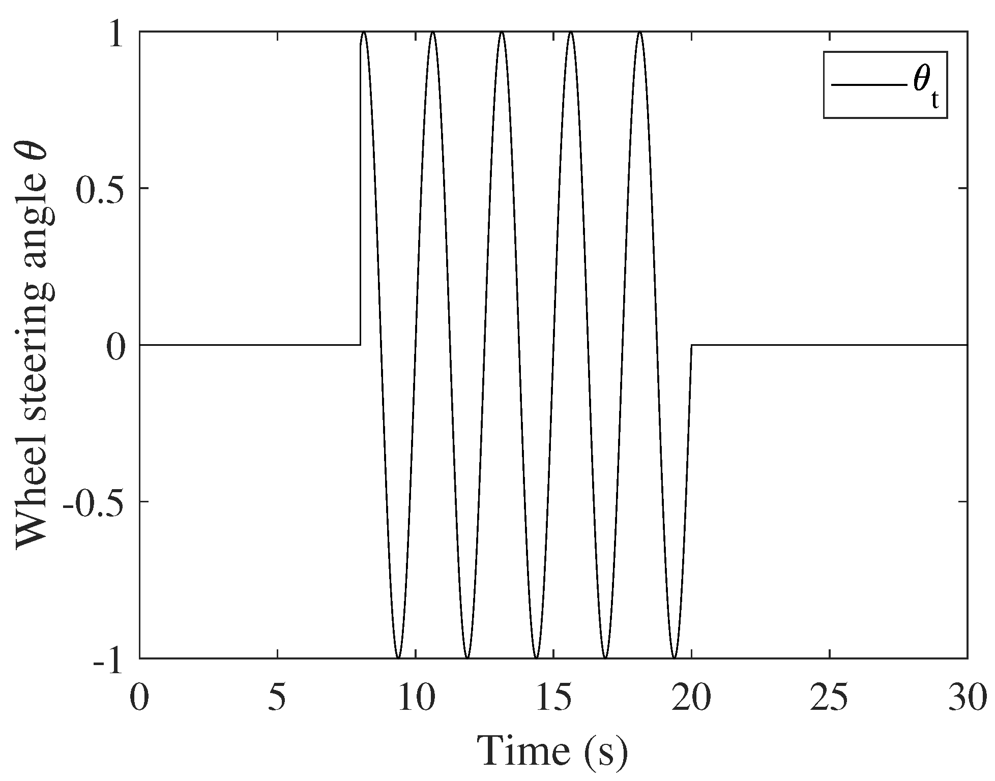
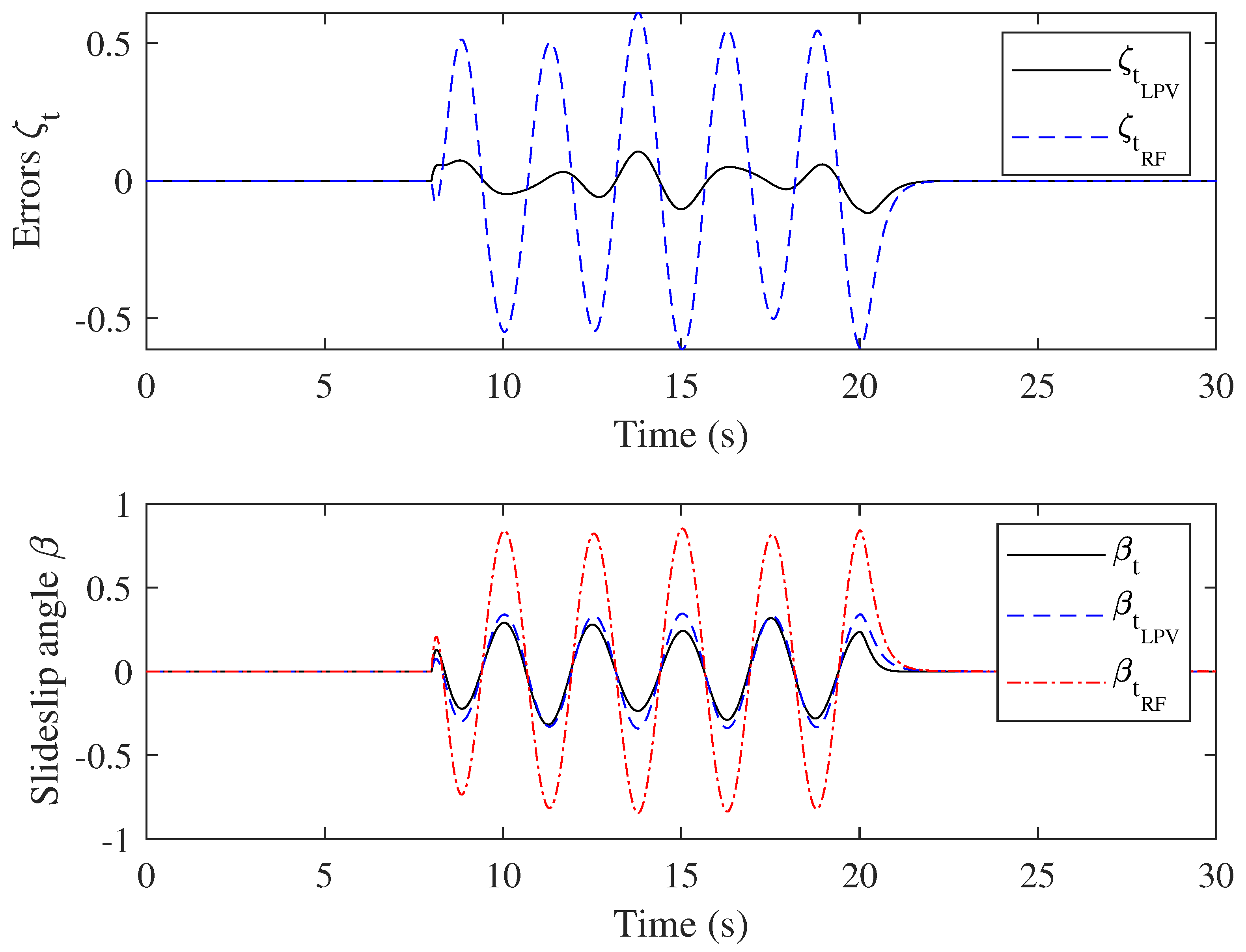
4. Simulation Examples

To demonstrate the benefits of the finite-frequency technique, particularly a low-frequency case for the E2P LPV filter design problem to estimate the vehicle sideslip angle, the minimum value of $\gamma$ for several low-frequency ranges was calculated, with the MATLAB LMI toolbox R2019a for the corresponding LPV filter matrices. The discussion focuses on comparing gain-scheduled and robust filter approaches in terms of E2P performance and examining the enhanced vehicle sideslip angle estimations in a low-frequency range. Since the results proposed in Corollary 1 and Corollary 2 provide solutions for the low-frequency (LF) interval, this simulation section concentrates on a low-frequency range filtering design for the vehicle sideslip angle estimation problem, which is an interesting application in ground vehicle systems.

In the simulations, $\Delta c_f$, $\Delta c_r$, and $v_x$ are defined by the following known ranges:

• $-0.4\le \Delta c_f\le 0.4$;
• $-0.4\le \Delta c_r\le 0.4$;
• $5\le$$v_x$$\le 30$$(\mathrm{m}/\mathrm{s})$.

By considering the defined interval of $v_x$ above, we obtained the results presented in

Table 3. $L_2-L_{\infty }$ computational performance results in terms of $\gamma$.

$\overline{\mathit{\delta }}$		0.1	1
$\omega \le$ 0.1	GSF	0.3982	0.8051
	RF	0.8620	1.7248
$\omega \le$ 1	GSF	0.9254	1.3608
	RF	1.6374	2.1607
$\omega \le$ 0.8$\pi$	GSF	1.8152	3.2889
	RF	2.1251	3.4080
$\omega \le$ 10	GSF	2.0771	3.5376
	RF	2.6645	4.8216
EF	GSF	2.0782	3.5415
	RF	2.7669	5.0071

, which provides the minimum values of $\gamma$ for various LF ranges, such that $\Delta c_f=0.1c_f$ and $\Delta c_r=0.1c_r$.

In Table 3, the effectiveness of the proposed method is demonstrated in terms of energy-to-peak minimization. Significant improvement can be observed in the obtained $L_2-L_{\infty }$ indices for the gain-scheduled filter (GSF) method provided by Corollary 1 compared to the robust filter (RF) approach presented by Corollary 2. This fact is highlighted in Remark 7, which provides an analysis point of view of the approach.

Moreover, the use of the FF method leads to better results in contrast to the EF (entire-frequency) method, and LPV filters provide better results than the robust filter design in terms of $L_2-L_{\infty }$ performance. Furthermore, the choice to study $L_2-L_{\infty }$ performance relies on treating the peak value of the signal, which can also depend on the fact that LPV filters vary, and the robust one is a constant parameter. Consequently, these results highlight the effectiveness of the LPV approach in reducing conservatism by including the same number of slack variables in contrast to the robust filter design approach.

Now, we consider the case of $\omega \le 0.8\pi$ to deal with another aspect of performance, which is the dynamic of $\overline{\delta }$. It is known that $\overline{\delta }$ represents the variation rate of the parameter $\delta$ such that the greater the $\overline{\delta }$, the greater and faster the variation in $\delta$. This can lead to an infeasible solution in terms of LMI conditions. To highlight this point, we provide the following table based on a comparative study considering $\gamma$ and a feasibility test (feasible or infeasible) of the RF and GSF approaches:

As a consequence,

Table 4. $\gamma$ index and feasibility test based on $\overline{\delta }$ rate variation (Inf: infeasible).

$\overline{\mathit{\delta }}$	0.1	1	1.38	1.39	1.49	1.5
GSF	1.8152	2.2889	6.30	6.41	8.1942	Inf
RF	2.1251	3.4080	7.3702	Inf	Inf	Inf

confirms the superiority of the GSF method compared to the RF one. This is shown first via the obtained values of $\gamma$ in both Table 3 and Table 4 and secondly based on the feasibility test of the proposed LMIs such that the GSF method is still feasible for larger values of $\overline{\delta }$. Moreover, the feasibility test highlights the robustness of the GSF in contrast to the RF method against fast variation in the LPV parameter $\delta$.

Let us move now to another point of performance. Dynamic simulations are now presented to show the effectiveness of estimating the sideslip angle. For this reason, the following filter parameters are used, corresponding to the frequency range $\omega \le 0.8\pi$:

• Gain-scheduled filter (GSF) parameters in (23) for $\overline{\delta }=1$:
  ${\mathbb{A}}_{f1}$ = $\left[\begin{array}{cc}-1.0430& -150.9255\\ 6.4580& -630.1210\end{array}\right]$, ${\mathbb{B}}_{f1}$ = $\left[\begin{array}{c}-149.9683\\ -630.1682\end{array}\right]$,
  ${\mathbb{C}}_{f1}$ = $\left[\begin{array}{cc}-0.8702& 0.0197\end{array}\right]$, $U_1$ = $\left[\begin{array}{cc}-0.3307& 0.0793\\ -0.0467& -0.0157\end{array}\right]$
  ${\mathbb{A}}_{f2}$ = $\left[\begin{array}{cc}-2.6200& -9.2789\\ 1.7396& -413.8975\end{array}\right]$, ${\mathbb{B}}_{f2}$ = $\left[\begin{array}{c}-8.8840\\ -413.0237\end{array}\right]$,
  ${\mathbb{C}}_{f2}$ = $\left[\begin{array}{cc}-0.8821& 0.0210\end{array}\right]$, $U_2$ = $\left[\begin{array}{cc}-0.3681& 0.0083\\ -0.0258& -0.0671\end{array}\right]$
  ${\mathbb{A}}_{f3}$ = $\left[\begin{array}{cc}-3.2785& 3.7480\\ 0.5131& -257.6864\end{array}\right]$, ${\mathbb{B}}_{f3}$ = $\left[\begin{array}{c}3.6574\\ -256.8073\end{array}\right]$,
  ${\mathbb{C}}_{f3}$ = $\left[\begin{array}{cc}-0.8882& 0.0245\end{array}\right]$, $U_3$ = $\left[\begin{array}{cc}-0.2526& -0.0035\\ -0.0022& -0.1089\end{array}\right]$
• Robust filter (RF) parameters in (25) for $\overline{\delta }=1$:
  ${\mathbb{A}}_f$ = ${10}^3\times \left[\begin{array}{cc}-0.0011& -0.4850\\ 0.0065& -1.7914\end{array}\right]$, ${\mathbb{B}}_f$ = ${10}^3\times \left[\begin{array}{c}-0.4841\\ -1.7915\end{array}\right]$, ${\mathbb{C}}_f$ = $\left[\begin{array}{cc}-0.8444& 0.0221\end{array}\right]$, U = $\left[\begin{array}{cc}-0.2733& 0.0740\\ 0.0302& -0.0240\end{array}\right]$

It is pointed out that the wheel steering angle in this application is only relevant at low frequencies, so the $L_2-L_{\infty }$ LPV filter tuned for the whole frequency range might not be adequate, as considering only low-frequencies may improve performance in this range. Thus, designing the $L_2-L_{\infty }$ LPV filter with the optimization for the LF range is suitable in this application. Therefore, dynamics were studied for low frequencies to illustrate the theoretical results.

As the filter aims to attenuate the effect of the wheel steering angle in the estimation error, some simulation results are now presented for the variations in the wheel steering angle (${\theta }_t$) presented in Figure 2.

Figure 3 presents the evolution of the estimation error ${\zeta }_t$ of the augmented systems and the corresponding output signals ${\mathrm{z}}_t$ and ${\widehat{\mathrm{z}}}_t$ for these variations in the steering angle.

Consequently, Figure 3 shows that the error signal goes to 0 in a steady state using LPV and robust filters. Furthermore, the obtained error signals ${\zeta }_{t_{LPV}}$ using the gain-scheduled filter are better than those obtained with the robust filter ${\zeta }_{t_{RF}}$. Figure 3 compares the estimations of the sideslip angle ${\beta }_t$ using the proposed LPV filter ${\beta }_{t_{LPV}}$ and by the robust filter ${\beta }_{t_{RF}}$. It can be seen that both filters provide adequate estimations of the sideslip angle, but the gain-scheduled LPV filter provides more accurate estimations.

Recall that Table 2 presents some comparisons of computational burden: for the example at hand ($N=2$, $N_z=1$), the developed approach only requires 19 decision variables, ensuring an extremely quick convergence. This is compared with 61 variables for the approach in [7]. Moreover, Table 4 presents a comparison between the RF and GSF, based on the derivative of $\rho$, showing that the proposed GSF method is feasible against larger variations in $\rho$.

We evaluated the accuracy of the proposed estimation method by quantifying the difference between estimated and actual values. For this reason, to ensure that estimations are as close as possible to desired values, we used the RMSE (root mean squared error) and MSE (mean squared error) metrics such that

$$MS{E}_{{\zeta }_{t_{LPV}}}=\sum _{i_1=1}^{n_1}{\displaystyle \frac{{\zeta }_{t_{LPV}}^2}{n_1}}$$

$$MS{E}_{{\zeta }_{t_{RF}}}=\sum _{i_1=1}^{n_1}{\displaystyle \frac{{\zeta }_{t_{Rf}}^2}{n_1}}$$

and

$$RMS{E}_{{\zeta }_{t_{LPV}}}=\sqrt{(}MS{E}_{{\zeta }_{t_{LPV}}})$$

$$RMS{E}_{{\zeta }_{t_{RF}}}=\sqrt{(}MS{E}_{{\zeta }_{t_{RF}}})$$

such that, in this case, $n_1=30$

The obtained results based on these metrics are listed in

Table 5. MSE and RMSE metrics of both methods, the GSF and RF.

	RMSE	MSE
GSF	0.1847	0.4298
RF	9.6868	3.1124

.

Based on Table 5 concerning the MSE and RMSE, as is well-known, this metric indicates overall model performance by averaging these squared errors and penalizes larger errors more heavily due to the squaring of residuals. One can see that the GSF provides smaller SME than the RF method. This fact has many interpretations to show up such as the following:

A smaller MSE means a closer estimation of the desired value. This means that the estimated dynamic related to $MS{E}_{{\zeta }_{t_{LPV}}}$ performs significantly better than the RF method related to $MS{E}_{{\zeta }_{t_{RF}}}$. On the other hand, the RF method has an average squared error that is about 7.24 times larger than that of the GSF method. This indicates that the first method makes larger prediction errors on average compared to the first method. This means that the GSF approach is more accurate and reliable for estimating the desired values. Otherwise, the RF method may either be poorly calibrated, underperforming, or inherently less suited for this kind of issue.

Moreover, based on the RMSE factor that represents the average magnitude of estimation errors, a smaller RMSE, which in this case is related to the GSF method ($RMS{E}_{{\zeta }_{t_{LPV}}}=0.1847$), suggests that this method is much more accurate than the second method ($RMS{E}_{{\zeta }_{t_{RF}}}$ = $9.6868$), as it has smaller estimation errors. This indicates that the second method performs far worse in terms of estimation accuracy.

All of the provided metrics above highlight the effectiveness of the LPV approach concerning both the estimation of the sideslip angle and the rejection of perturbations represented by the $L_2-L_{\infty }$ index.

In summary, it has been shown that the proposed LPV $L_2-L_{\infty }$ filtering approach is a valuable filtering technique for sideslip angle estimation, achieving better results than robust filtering.

5. Conclusions

The issue of estimating a ground vehicle’s sideslip angle has prompted the design of gain-scheduled E2P filters that optimize a performance indicator in finite-frequency ranges. From an uncertain LPV model of the sideslip angle, conditions for asymptotic stability were presented using an FF formulation. Slack matrices provide extra degrees of freedom, reducing the E2P index. The FF technique was merged with the LPV filter design methodology with gain-scheduled filter parameters obtained from a set of LMIs. Simulations demonstrate the effectiveness of the LPV approach in comparison to the robust filtering method, especially in terms of the minimization of error peak values. The proposed results improve upon previous results in filtering for vehicles, such as those presented in [16] and the references therein, as they are based on gain-scheduling, which allows them to adapt to the inherent system nonlinearities. Moreover, this study focused on optimizing the low-frequencies region, which is relevant in practice. This work provides a starting point for future works involving cyber-attack filtering for LPV systems.

References

1. Lenzo, B.; Zanchetta, M.; Sorniotti, A.; Gruber, P.; De Nijs, W. Yaw rate and sideslip angle control through single input single output direct yaw moment control. IEEE Trans. Control. Syst. Technol. 2020, 29, 124–139. [Google Scholar] [CrossRef]
2. Zheng, B.; Anwar, S. Yaw stability control of a steer-by-wire equipped vehicle via active front wheel steering. Mechatronics 2009, 19, 799–804. [Google Scholar] [CrossRef]
3. Zhang, H.; Wang, R.; Wang, J. Sideslip angle estimation of an electric ground vehicle via finite-frequency H approach. In Robust Gain-Scheduled Estimation and Control of Electrified Vehicles via LPV Technique; Springer: Berlin/Heidelberg, Germany, 2023; pp. 75–95. [Google Scholar]
4. Liu, C.; Yao, J. Sideslip Angle Estimation for Lateral Vehicle Control with Delayed Output Measurements. In Proceedings of the 2022 International Conference on Advanced Robotics and Mechatronics (ICARM), Guilin, China, 9–11 July 2022; IEEE: Piscataway, NJ, USA, 2022; pp. 866–869. [Google Scholar]
5. Zhang, H.; Zhang, G.; Wang, J. Sideslip Angle Estimation of an Electric Ground Vehicle via Finite-Frequency H Approach. IEEE Trans. Transp. Electrif. 2015, 2, 200–209. [Google Scholar] [CrossRef]
6. Chang, X.H.; Liu, Y. Robust H Filtering for Vehicle Sideslip Angle With Quantization and Data Dropouts. IEEE Trans. Veh. Technol. 2020, 69, 10435–10445. [Google Scholar] [CrossRef]
7. Hellani, D.E.; Hajjaji, A.E.; Ceschi, R.; Aitouche, A. Sideslip Angle Estimation of Ground Vehicles in a Finite Frequency Domain Through H Approach. In Proceedings of the 2018 26th Mediterranean Conference on Control and Automation (MED), Zadar, Croatia, 19–22 June 2018; IEEE: Piscataway, NJ, USA, 2018; pp. 1–9. [Google Scholar]
8. El Hellani, D.; El Hajjaji, A.; Ceschi, R. Finite frequency H filter design for TS fuzzy systems: New approach. Signal Process. 2018, 143, 191–199. [Google Scholar] [CrossRef]
9. Iwasaki, T.; Hara, S. Generalized KYP Lemma: Unified frequency domain inequalities with design applications. IEEE Trans. Autom. Control 2005, 50, 41–59. [Google Scholar] [CrossRef]
10. Frezzatto, L.; Oliveira, R.C.; Peres, P.L. L2-gain filter design for continuous-time LPV systems in finite frequency domain. IFAC-PapersOnLine 2018, 51, 161–166. [Google Scholar] [CrossRef]
11. Gao, H.; Li, X. Robust Filtering for Uncertain Systems; Springer: Berlin/Heidelberg, Germany, 2016. [Google Scholar]
12. Zhang, H.; Mehr, A.S.; Shi, Y. Improved robust energy-to-peak filtering for uncertain linear systems. Signal Process. 2010, 90, 2667–2675. [Google Scholar] [CrossRef]
13. Wilson, D.A. Convolution and Hankel operator norms for linear systems. IEEE Trans. Autom. Control 1989, 34, 94–97. [Google Scholar] [CrossRef]
14. Gyurkovics, É.; Takács, T. Robust energy-to-peak filter design for a class of unstable polytopic systems with a macroeconomic application. Appl. Math. Comput. 2021, 420, 126729. [Google Scholar] [CrossRef]
15. Zhang, H.; Wang, J. Robust gain-scheduling control of vehicle lateral dynamics through AFS/DYC. In Modeling, Dynamics and Control of Electrified Vehicles; Elsevier: Amsterdam, The Netherlands, 2018; pp. 339–368. [Google Scholar]
16. Liao, S. Robust H filtering and time-varying delay compensation for car suspension systems: A comprehensive approach to reduced disturbance and enhanced estimation. Multiscale Multidiscip. Model. Exp. Des. 2024, 7, 2343–2357. [Google Scholar] [CrossRef]
17. Zhang, H.; Huang, X.; Wang, J.; Karimi, H.R. Robust energy-to-peak sideslip angle estimation with applications to ground vehicles. Mechatronics 2015, 30, 338–347. [Google Scholar] [CrossRef]
18. Cao, X.; Xu, T.; Tian, Y.; Ji, X. Gain-scheduling LPV synthesis H robust lateral motion control for path following of autonomous vehicle via coordination of steering and braking. Veh. Syst. Dyn. 2023, 61, 968–991. [Google Scholar] [CrossRef]
19. Aslam, M.S.; Bilal, H.; Anjum, Z. Gain-scheduled filter design with different time delays for TS fuzzy systems. Trans. Inst. Meas. Control 2024, 01423312241274009. [Google Scholar] [CrossRef]
20. Li, X.J.; Yang, G.H. Finite Frequency L2L Filtering of TS Fuzzy Systems With Unknown Membership Functions. IEEE Trans. Syst. Man Cybern. Syst. 2016, 47, 1884–1897. [Google Scholar] [CrossRef]
21. Todorov, M.G. A New Approach to the Energy-to-Peak Performance Analysis of Continuous-Time Markov Jump Linear Systems. IEEE Control Syst. Lett. 2024, 8, 1024–1029. [Google Scholar] [CrossRef]
22. Yu, H.; Hu, J.; Song, B.; Liu, H.; Yi, X. Resilient energy-to-peak filtering for linear parameter-varying systems under random access protocol. Int. J. Syst. Sci. 2022, 53, 2421–2436. [Google Scholar] [CrossRef]
23. van Waarde, H.J.; Camlibel, M.K. A matrix Finsler’s lemma with applications to data-driven control. In Proceedings of the 2021 60th IEEE Conference on Decision and Control (CDC), Austin, TX, USA, 13–17 December 2021; IEEE: Piscataway, NJ, USA, 2021; pp. 5777–5782. [Google Scholar]
24. Hu, J.; Chen, W.; Wu, Z.; Chen, D.; Yi, X. Design of protocol-based finite-time memory fault detection scheme with circuit system application. IEEE Trans. Syst. Man Cybern. Syst. 2024, 54, 3110–3123. [Google Scholar] [CrossRef]
25. Lozia, Z. Vehicle dynamics and motion simulation versus experiment. SAE Trans. 1998, 107, 344–360. [Google Scholar]
26. Kutluay, E.; Winner, H. Validation of vehicle dynamics simulation models—A review. Veh. Syst. Dyn. 2014, 52, 186–200. [Google Scholar] [CrossRef]
27. Kim, J. Effect of vehicle model on the estimation of lateral vehicle dynamics. Int. J. Automot. Technol. 2010, 11, 331–337. [Google Scholar] [CrossRef]
28. Das, S.; Shrudhanidhi. Vehicle Dynamics Modelling: Lateral and Longitudinal. In Proceedings of the 2021 8th International Conference on Signal Processing and Integrated Networks (SPIN), Noida, India, 26–27 August 2021; pp. 407–412. [Google Scholar] [CrossRef]
29. Geromel, J.C.; Colaneri, P. Robust stability of time varying polytopic systems. Syst. Contro. Lett. 2006, 55, 81–85. [Google Scholar] [CrossRef]
30. Iwasaki, T.; Hara, S.; Fradkov, A.L. Time domain interpretations of frequency domain inequalities on (semi) finite ranges. Syst. Control Lett. 2005, 54, 681–691. [Google Scholar] [CrossRef]
31. de Oliveira, M.C.; Skelton, R.E. Stability tests for constrained linear systems. In Perspectives in Robust Control; Springer: Berlin/Heidelberg, Germany, 2001; pp. 241–257. [Google Scholar]
32. Khargonekar, P.P.; Petersen, I.R.; Zhou, K. Robust stabilization of uncertain linear systems: Quadratic stabilizability and H control theory. IEEE Trans. Autom. Control 1990, 35, 356–361. [Google Scholar] [CrossRef]
33. Zoulagh, T.; El Haiek, B.; Hmamed, A.; El Hajjaji, A. Homogenous polynomial H filtering for uncertain discrete-time systems: A descriptor approach. Int. J. Adapt. Control Signal Process. 2018, 32, 378–389. [Google Scholar] [CrossRef]
34. El Haiek, B.; Zoulagh, T.; Hmamed, A.; El Adel, E.M. Polynomial static output feedback H control for continuous-time linear systems via descriptor approach. Int. J. Innov. Comput. Inf. Control 2017, 13, 941–952. [Google Scholar]
35. Lofberg, J. YALMIP: A toolbox for modeling and optimization in MATLAB. In Proceedings of the 2004 IEEE international conference on robotics and automation (IEEE Cat. No. 04CH37508), New Orleans, LA, USA, 26 April–1 May 2004; IEEE: Piscataway, NJ, USA, 2004; pp. 284–289. [Google Scholar]
36. Sturm, J.F. Using SeDuMi 1.02, a MATLAB toolbox for optimization over symmetric cones. Optim. Methods Softw. 1999, 11, 625–653. [Google Scholar] [CrossRef]
Figure 1. Schema of the simplified lateral dynamics model.
Symmetry 16 01627 g001
Figure 2. Evolution of the wheel steering angle θ used in the simulations to test the response to variations in this angle.
Symmetry 16 01627 g002
Figure 3. Comparison of the estimation errors ζ t and the sideslip angles β obtained using the proposed LPV and a robust filter to demonstrate the better performance of the proposed LPV filter.
Symmetry 16 01627 g003