Robustness Analysis of Exponential Synchronization in Complex Dynamic Networks with Deviating Argumentsand Parameter Uncertainties

Abstract

In the paper, we study the robust synchronization of complex dynamic networks (CDNs) with deviating arguments and parameter uncertainties via self-feedback control, the model involves both advanced and delayed arguments. In addition, based on the Gronwall inequality and inequality techniques, we derive upper bounds on the length of the arguments and the magnitude of the parameters, when the parameters and arguments of CDNs are below the upper bounds, the CDNs continue to exhibit exponential synchronization. In comparison to linear matrix inequalities and Lyapunov’s method in the existing literature, we obtain elaborate bounds. Finally, Several simple examples can demonstrate the effectiveness of the results.

1. Introduction

Complex dynamic networks (CDNs) are neural networks with a complex structure composed of many nodes coupled with edges, and each node is a basic element of CDNs. Consequently, the entire networks exhibit different dynamic behaviors than isolated nodes. CDN models have been widely used to describe many natural and artificial systems, such as the internet networks, power grids, neural networks and biological networks [1,2,3,4,5,6,7,8].

In fact, synchronization is a common phenomenon in nature. For example, the clustering activity of bees in the forest can be considered as a synchronized behavior. In recent years, the synchronization problem of CDNs has become an emerging research field and attracted substantial attentions [9,10,11,12]. In order to achieve synchronization of CDNs, many scholars have proposed many control schemes, such as pinning control, impulsive control and event-triggered control [13,14,15,16].

The above investigations concentrate on the synchronization or stability analysis of delayed CDNs. In the fields of economics, biology, and physics, the past and future events serve as references for current decision-making. Therefore, it is significant to discuss models involving delay and advanced alternating differential equations. CDNs with deviating arguments (DAs) are considered to be the unification of delayed and advanced systems. In addition, it is also the combination of continuous and discrete system [17,18,19,20,21]. By substituting the time delays of CDNs with DAs, the system will have more sophisticated structure and widespread applications. Hence, it is significant and meaningful to investigate the robust synchronization of CDNs with DAs. In [18], the Mittag-Leffler stability of fractional-order neural networks with generalized piecewise constant arguments is investigated. The impulsive control strategy is employed to achieve synchronization of CDNs with DAs in [19]. In [20], the robust stability of fuzzy cellular neural networks with DAs is investigated by designing suitable controllers.

On the one hand, the coupling weights between CDNs depend on the resistance and capacitance values, due to the variation of charge flow in the systems, the resistance and capacitance of the systems will also evolve. On the other hand, neural networks exhibit parameter uncertainty due to modeling uncertainty, which makes it challenging to describe the system with constant parameters [22,23,24,25]. Consequently, the parameter uncertainties (PUs) of the connection weights are inevitable. Models of CDNs with arguments and uncertainties can lead to chaotic, oscillatory, and instability, and how much argument length and parameter magnitude can cause the systems to unsynchronized systems, the subject rarely discussed in previous literatures.

It is well known that if DAs and PUs exceed the certain thresholds, it will lead to system instability, oscillation or performance degradation. How much longer argument and parameter scales will maintain the exponential synchronization of the system? The main contributions of this paper include the following aspects:

• In the paper, we study the robust synchronization of CDNs with DAs. Compared with systems with ordinary time delays, the system discussed in this paper involves both delayed and advanced coupling, and we employ an unified model to describe the finite speed of signal propagation and to predict the behavior of nodes.
• We introduce upper bounds for the argument length and parameter size in CDNs by employing Gronwall inequalities and inequality techniques.
• Massive complex networks are scale-free, meaning that most nodes are disconnected, but a few have many connections. In addition, the connection matrix in the model of CDNs are all symmetric, i.e., if nodes i and j are connected and disconnected, the adjacency matrix parameters are 0 and 1, respectively. This matrix is described in the model establishment in Section 2 and the simulation in Section 4.

The rest of this paper is arranged as follows. In Section 2, some preliminaries on the model of complex dynamic networks and lemmas are presented. In Section 3, we transform systems with arguments into ordinary systems. Furthermore, upper bounds on the length of the arguments and the magnitude of the parameters were derived utilising Grunwald inequality. Two numerical examples are exhibited to illustrate the effectiveness of the obtained results in Section 4. This paper is concluded and future possible works are given in Section 5.

2. Preliminaries

2.1. Notation

The following are the standard notations used in this article. Let ${\mathbb{R}}^n$ is n-dimensional Euclidean space, $\mathbb{R}$ be the space of real numbers, the superscript T represents the transpose of vector or matrix. ${\mathbb{R}}^{+}$ is the set of positive real number, $\mathbb{N}$ represents integers, $\left|\right|\chi \left(t\right)\left|\right|$ is the norm of vector $\chi \left(t\right)$, where $\chi \left(t\right)\in {\mathbb{R}}^n$ and $\left|\right|\chi \left(t\right)\left|\right|={\sum }_{p=1}^n\left|\chi \left(t\right)\right|$, the norm $\left|\right|A\left|\right|$ of the matrix A is given by $\left|\right|A\left|\right|$, where $A={max}_{1\le q\le n}{\sum }_{p=1}^n\left|a_{pq}\right|$.

The interactions of CDNs can be characterized by graph $\mathbb{G}=(\mathbb{V},E,A)$, where $\mathbb{V}$ are a set of CDNs. $E\in \mathbb{V}\times \mathbb{V}$ represents a series of interaction edges, and A is a coupling matrix.

For two real-valued sequences ${\varrho }_k$, ${\xi }_k$, $k\in \mathbb{N}$. ${\varrho }_k<{\varrho }_{k+1}, {\varrho }_k\le {\xi }_k\le {\varrho }_{k+1}$ for all $k\in \mathbb{N}$ with ${\varrho }_k\to \infty$ as $k\to \infty$.

2.2. Preliminary Preparation

Consider a complex dynamical network with mixed coupling as follow,

$$\begin{array}{cc}\hfill {\dot{x}}_p\left(t\right)=& f\left(x_p\left(t\right)\right)+c\sum _{q=1}^n(a_{pq}+△a_{pq}\left(t\right))x_q\left(t\right)\hfill \\ \hfill & +c\sum _{q=1}^n{b}_{pq}{x}_q\left(\gamma \left(t\right)\right)+{\varpi }_p,\hfill \\ \hfill x_p\left(t_0\right)=& w_0,\hfill \end{array}$$

(1)

where $p=1,\dots ,n$ is the state vector of the ith dynamical node, the nonlinear function $f(·)\in {\mathcal{C}}^1([t_0,+\infty ],\mathbb{R})$ is continuous activation function, ${\varpi }_p$ is control input, c is a coupling strength, the Laplacian matrix $\tilde{A}=\left(a_{ij}\right),\tilde{B}=\left(b_{ij}\right)\in {\mathbb{R}}^{n\times n}$ describes the topological structure of the network with

$$\begin{array}{c}\hfill a_{pp}=-\sum _{q=1}^n{a}_{pq},b_{pp}=-\sum _{q=1}^n{b}_{pq},p\ne q.\end{array}$$

If $(x_p,x_q)\in E$, then $a_{pq}=\pm 1$, otherwise, $a_{pq}=0$. There isn’t self-loops in $\mathbb{G}$, i.e., $a_{pp}=0$. Moreover, $a_{pq}=a_{qp}\ge 0,\forall p,q$. The choice of configuration matrices for complex dynamic networks is related to the direct links between nodes, and the topology of the network may have a certain symmetry.

We always set $\gamma \left(t\right)={\xi }_k$ on $({\varrho }_k,{\varrho }_{k+1}]$, when $t\in (t_k,t_{k+1}]$, if ${\xi }_k>t$, then the coupling is advanced, and if ${\xi }_k<t$, then the coupling is delayed. In this paper, the deviation parameter $\gamma \left(t\right)$ is discontinuous. Consequently, the right-hand side of the CDNs (1) has a discontinuity at the moment ${\varrho }_k,k\in \mathbb{N}$. Therefore, we make the solution function of the equation continuous and continuously differentiable in the interval $({\varrho }_k,{\varrho }_{k+1}]$.

The initial conditions are as follows

$$\begin{array}{c}\hfill x_p\left(t_0\right)=\varphi ,\end{array}$$

where $t_0\in [-\rho ,t_0]$.

Remark 1. 

In [19], the CDNs (1) is demonstrated to have a unique solution $x\left(t\right)$ on the interval $[{\varrho }_k,{\varrho }_{k+1}]$. Moreover, k can take any value on $\mathbb{N}$. Consequently, the solution of system (1) exists on $\mathbb{R}$.

The $s\left(t\right)$ is an arbitrary state, which is also an isolated node of the CDN (1) such that

$$\begin{array}{c}\hfill \dot{s}\left(t\right)=f\left(s\left(t\right)\right).\end{array}$$

(2)

The linear controller is designed as

$$\begin{array}{c}\hfill {\varpi }_p\left(t\right)={\varsigma }_p(x_p\left(t\right)-s\left(t\right)),p=1,\cdots ,n,\end{array}$$

(3)

where ${\varsigma }_p$ is positive constant.

Combining $\left(1\right)$ and $\left(2\right)$, the $e_p\left(t\right)=x_p\left(t\right)-s\left(t\right)$ represents the errors relative to the isolated node, then,

$$\begin{array}{cc}\hfill {\dot{e}}_p\left(t\right)=& f\left(e_p\left(t\right)\right)+c\sum _{q=1}^n(a_{pq}+△a_{pq}\left(t\right))e_q\left(t\right)\hfill \\ \hfill & +c\sum _{q=1}^n{b}_{pq}{e}_q\left(\gamma \left(t\right)\right)+{\varsigma }_p{e}_p\left(t\right),\hfill \end{array}$$

(4)

in which $f\left(e_p\left(t\right)\right)=f\left(x_p\left(t\right)\right)-f\left(s\left(t\right)\right)$, the initial values are as follows

$$\begin{array}{c}\hfill e_p\left(t_0\right)=\phi .\end{array}$$

Then CDNs (4) can be rewritten in a compact matrix form

$$\begin{array}{cc}\hfill & \dot{e}\left(t\right)=F\left(e\left(t\right)\right)+c(A+\widehat{A}\left(t\right))e\left(t\right)+cBe\left(\gamma \left(t\right)\right)+We\left(t\right).\hfill \\ \hfill & e\left(t_0\right)=e_0\hfill \end{array}$$

(5)

$e\left(t\right)={(e_1\left(t\right),\dots ,e_n\left(t\right))}^T$, $e\left(\gamma \left(t\right)\right)={(e_1\left(t\right),\dots ,e_n\left(t\right))}^T$, $F\left(e\left(t\right)\right)={(f\left(e_1\left(t\right)\right),\dots ,f\left(e_n\left(t\right)\right))}^T$, $t_0\in {\mathbb{R}}^{+}$, $e_0$ is the initial condition. $A=I_n⨂\tilde{A}$, $B=I_n⨂\tilde{B}$, $W={\left({\varsigma }_p\right)}_{n\times n}$ is a diagonal matrix, $\widehat{A}\left(t\right)=(△a_{pq}\left(t\right))\in {\mathbb{R}}^{n\times n}$.

In addition, the function f in (4) satisfies the following global Lipschitz condition and $f\left(0\right)=0$.

Assumption 1. 

Assume that there exists a nonnegative constant p, such that

$$\begin{array}{c}\hfill |f\left(v_p\right)-f\left(w_p\right)|\le l_p|v_p-w_p|,\end{array}$$

where the activation function $f_p(p\in 1,2,\dots ,n)$ is global Lipschitz-continuous, $w_p,v_p\in \mathbb{R}$.

The original system with the controller is

$$\begin{array}{cc}\hfill & \dot{z}\left(t\right)=F\left(z\left(t\right)\right)+cAz\left(t\right)+cBz\left(t\right)+We\left(t\right).\hfill \\ \hfill & z\left(t_0\right)=z_0\hfill \end{array}$$

(6)

where $z\left(t\right)={(z_1\left(t\right),\dots ,z_n\left(t\right))}^T$, $e_0$ is the initial condition of (6).

The following lemmas and assumptions will be needed through out the paper:

Definition 1 

([26]). If we have the following inequality,

$$\begin{array}{c}\hfill |x\left(t\right)-s\left(t\right)|\le \theta \left|\phi \right|exp(-\vartheta (t-t_0)),\end{array}$$

where $t>t_0$, φ is initial conditions, $\theta ,\vartheta >0$. Then, the state of system (5) is said to be globally exponentially stable (ESt).

The symmetry of CDNs topology can influence the dynamical behaviour of the networks. For example, the symmetric networks structure may lead to the emergence of group synchronisation phenomena in which nodes in the network exhibit coordinated behaviour. We focus on ESy between nodes of complex networks in this paper.

Assumption 2. 

There exists a positive constant ξ that satisfies ${\varrho }_{k+1}-{\varrho }_k\le \varrho$, for all $k\in \mathbb{N}$.

Assumption 3. 

The parameter uncertainties and bounded, defined by

$$\begin{array}{c}\hfill △a_{pq}\left(t\right)\le M_{pq}^{\left(1\right)},\end{array}$$

where $M_{pq}^{\left(1\right)}>0$.

Assumption 4. 

$h_2\varrho -h_1\varrho (1+h_2\varrho )exp\left\{h_1\varrho \right\}<1$.

Assumption 5. 

$c\varrho \left|B\right|+\varrho \left(c\right(\left|A\right|+|A^{*}\left|\right)+|\overline{K}\left)\right(1+c\varrho \left|B\right|)exp\{\varrho \left(c\right(\left|A\right|+|A^{*}\left|\right)+|\overline{K}\left)\right\}<1$.

Lemma 1 

([27]). Suppose $\vartheta \left(t\right)$, $\theta \left(t\right)$, and $e\left(t\right)$ are continuous real-valued functions, and $\theta \left(t\right)$ is integrable over the interval $I=[t_0,t]$, if $\vartheta \left(t\right)\ge 0$ and $u\left(t\right)$ satisfies

$$\begin{array}{c}\hfill e\left(t\right)\le \theta \left(t\right)+{\int }_{t_0}^t\vartheta \left(s\right)e\left(s\right)ds,\end{array}$$

then,

$$\begin{array}{c}\hfill e\left(t\right)\le \theta \left(t\right)+{\int }_{t_0}^t\theta \left(s\right)\vartheta \left(s\right)exp\left({\int }_s^t\vartheta \left(r\right)dr\right)ds,\end{array}$$

where $t>t_0$.

In addition, if $\theta \left(t\right)$ is non-decreasing, then

$$\begin{array}{c}\hfill e\left(t\right)\le \theta \left(t\right)exp\left({\int }_{t_0}^t\vartheta \left(s\right)ds\right).\end{array}$$

Lemma 2. 

Under Assumption 1, if $e\left(t\right)$ is the solution of system (5), then

$$\begin{array}{c}\hfill \left|e\right(\gamma \left(t\right)\left)\right|\le \lambda \left|e\right(t\left)\right|,\end{array}$$

(7)

holds on $t\in {\mathbb{R}}^{+}$, where $\lambda ={(1-h_2\varrho -h_1\varrho (1+h_2\varrho )exp\left\{h_1\varrho \right\})}^{-1}$, $h_1=\left|L\right|+c\left(\right|A|+|A^{*}\left|\right)+\left|W\right|$, $h_2=c\left|B\right|$, $L={\left(l_p\right)}_{n\times n}$ is a diagonal weight, $A^{*}={sup}_{t\ge t_0}\widehat{A}\left(t\right)$.

Proof. 

For $\gamma \left(t\right)={\xi }_k$, and $t\in \left({\varrho }_k,{\varrho }_{k+1}\right]$,

$$\begin{array}{cc}\hfill e\left(t\right)=& e\left({\xi }_k\right)+{\int }_{{\xi }_k}^{t}F\left(e\left(s\right)\right)+c(A+\widehat{A}\left(s\right))e\left(s\right)\hfill \\ & +cBe\left({\xi }_k\right)+We\left(s\right)ds.\hfill \end{array}$$

For $t\in [{\xi }_k,{\varrho }_{k+1}]$,

$$\begin{array}{cc}\hfill \left|e\right(t\left)\right|\le & |e\left({\xi }_k\right)|+{\int }_{{\xi }_k}^t\left(\right|F\left(e\left(s\right)\right)|+c(\left|A\right|+|\widehat{A}\left(s\right)\left|\right)|e\left(s\right)|\hfill \\ & +c\left|B\right||e\left({\xi }_k\right)|+|W\left|\right|e\left(s\right)\left|\right)ds\hfill \\ \hfill \le & (1+h_2\varrho )|e\left({\xi }_k\right)|+{\int }_{{\xi }_k}^t{h}_1\left|e\left(s\right)\right|ds,\hfill \end{array}$$

where $h_1=\left|L\right|+c\left(\right|A|+|A^{*}\left|\right)+\left|W\right|$, $h_2=c\left|B\right|$. □

According to Lemma 1,

$$\begin{array}{c}\hfill \left|e\left(t\right)\right|\le \left((1+h_2\varrho )|e\left({\xi }_k\right)\right)|exp\left(h_1\varrho \right).\end{array}$$

(8)

By the similar method above,

$$\begin{array}{cc}\hfill \left|e\right({\xi }_k\left)\right|\le & \left|e\left(t\right)\right|+{\int }_{{\xi }_k}^t\left(\right|F\left(e\left(s\right)\right)|+c(\left|A\right|+|\widehat{A}\left(s\right)\left|\right)\left|e\left(s\right)\right|\hfill \\ \hfill & +c\left|B\right||e\left({\xi }_k\right)|+|W\left|\right|e\left(s\right)\left|\right)ds\hfill \\ \hfill \le & \left|e\left(t\right)\right|+h_2\varrho |e\left({\xi }_k\right)|+{\int }_{{\xi }_k}^t{h}_1\left|e\left(s\right)\right|ds\hfill \\ \hfill \le & \left|e\left(t\right)\right|+h_2\varrho \left|e\left({\xi }_k\right)\right|\hfill \\ \hfill & +h_1\varrho \left((1+h_2\varrho )\left|e\left({\xi }_k\right)\right|\right)exp\left(h_1\varrho \right).\hfill \end{array}$$

(9)

From (9), we have

$$\begin{array}{c}\hfill \left(1-h_2\varrho -h_1\varrho (1+h_2\varrho )exp\left\{h_1\varrho \right\}\right)|x\left({\xi }_k\right)|\le |x\left(t\right)|.\end{array}$$

(10)

From Assumption 4,

$$\begin{array}{cc}\hfill \left|z\right({\xi }_k\left)\right|& \le \lambda \left|x\right(t\left)\right|,\hfill \end{array}$$

(11)

where $\lambda =1/(1-h_2\varrho -h_1\varrho (1+h_2\varrho )exp\left\{h_1\varrho \right\})$, for $t\in ({\varrho }_k,{\varrho }_{k+1}]$. By the randomness of t and k, it follows that (11) holds for all $t\in {\mathbb{R}}^{+}$.

Remark 2. 

When considering CDN (1) on the interval $({\varrho }_k,{\varrho }_{k+1}]$, where $k\in \mathbb{N}$, if ${\varrho }_k\le t<{\xi }_k$, CDN (1) behaves as an advanced system. Conversely, if ${\xi }_k<t\le {\varrho }_{k+1}$, CDN (1) behaves as a retarded system. In other words, Equation (1) can alternate between advanced and retarded arguments.

Remark 3. 

By virtue of Lemma 1, we have obtained a method to transform state vector $x\left(\gamma \right(t\left)\right)$ into regular state vector $x\left(t\right)$.

3. Main Results

The CDNs with parameter uncertainty are as follows:

$$\begin{array}{c}\hfill \dot{e}\left(t\right)=F\left(e\left(t\right)\right)+c(A+\widehat{A}\left(t\right))e\left(t\right)+We\left(t\right),\end{array}$$

(12)

where $e\left(t\right)={(e_1\left(t\right),\dots ,e_n\left(t\right))}^T\in {\mathbb{R}}^n$ is the state vector of the nodes, $e_0\in {\mathbb{R}}^n$ is the initial condition, A, $\widehat{A}$, W and $F(·)$ are the same as in Section 2, The activation function $f(·)$ satisfies Assumption 1 and $f\left(0\right)=0$.

The original system is

$$\begin{array}{c}\hfill \dot{z}\left(t\right)=F\left(z\left(t\right)\right)+cAz\left(t\right)+Wz\left(t\right),\end{array}$$

(13)

where $z\left(t\right)={(z_1\left(t\right),\dots ,z_n\left(t\right))}^T\in {\mathbb{R}}^n$ is the state variable without uncertainty.

In order to explore the effect of the PUs on the synchronization of the systems. That is, how large parameter matrices will desynchronize the system. Consequently, we have the following theorem.

Theorem 1. 

The Assumptions 1 and 3 hold. If the CDNs (13) is globally exponentially stability (ESt), $|A^{*}|<min\{\beth ,|M^{\left(1\right)}\left|\right\}$, then CDNs (12) still remains to be globally ESt, the CDNs (1) to isolated node (2) is globally exponential synchronization (ESy), where ℶ is the unique nonnegative solution of the transcendental equation:

$$\begin{array}{c}\hfill {{\rm Y}}_{1}exp\left(2{{\rm Y}}_2\mathbb{T}\right)+\theta exp(-\vartheta \mathbb{T})=1,\end{array}$$

(14)

where ${{\rm Y}}_1=c\left|A^{*}\right|\theta /\vartheta$, ${{\rm Y}}_2=\left|L\right|+c\left(\right|A|+|A^{*}\left|\right)+\left|W\right|$, $M^{\left(1\right)}=\left(M_{pq}^{\left(1\right)}\right)\in {\mathbb{R}}^{n\times n}$, $\mathbb{T}>(ln\theta )/\vartheta$.

Proof. 

Assume $e_0=z_0$, $e_0$ and $z_0$ are (12) and (13) initial conditions, respectively.

$$\begin{array}{cc}\hfill \left|z\right(t)-e(t\left)\right|=& \left|{\int }_{t_0}^t\right((F\left(z\left(s\right)\right)-F\left(e\left(s\right)\right))+c(A+\widehat{A}\left(s\right))(z\left(s\right)\hfill \\ & -e\left(s\right))+W(z\left(s\right)-e\left(s\right)\left)\right)ds|\hfill \\ \hfill \le & {\int }_{t_0}^t\left(\right|F\left(z\left(s\right)\right)-F\left(e\left(s\right)\right)|+c|A\left|\right||z\left(s\right)-e\left(s\right)|\hfill \\ & +|\widehat{A}\left|\right|z\left(s\right)|+|W\left|\right|z\left(s\right)-e\left(s\right)\left|\right)ds.\hfill \end{array}$$

Then, $t_0\le t\le t_0+2\mathbb{T}$,

$$\begin{array}{cc}\hfill \left|z\right(t)-e(t\left)\right|\le & {\int }_{t_0}^t\left(\right|L\left|\right|z\left(s\right)-e\left(s\right)|+c|A\left|\right|z\left(s\right)-e\left(s\right)|\hfill \\ & +c|\widehat{A}\left(s\right)\left|\right|z\left(s\right)-e\left(s\right)|+c|\widehat{A}\left(t\right)\left|z\left(s\right)\right|\hfill \\ & +\left|W\right|\left|z\right(s)-e(s\left)\right|)ds\hfill \\ \hfill \le & {\int }_{t_0}^t\left(\right(\left|L\right|+c\left(\right|A|+|A^{*}\left|\right)+\left|W\right|\left)\right|z\left(s\right)-e\left(s\right)|\hfill \\ & +c|A^{*}\left|\right|z\left(s\right)\left|\right)ds\hfill \end{array}$$

Then, (13) is locally ESt,

$$\begin{array}{cc}\hfill \left|z\right(t)-e(t\left)\right|\le & \left(\right|L|+c(\left|A\right|+|A^{*}\left|\right)+\left|W\right|){\int }_{t_0}^t|z\left(s\right)-e\left(s\right)|ds\hfill \\ & +c|A^{*}\left|\right|z_0|\theta /\vartheta .\hfill \end{array}$$

From the Lemma 1,

$$\begin{array}{c}\hfill |z\left(t\right)-e\left(t\right)|\le {{\rm Y}}_1\left|z_0\right|exp\left(2\mathbb{T}{{\rm Y}}_2\right),\end{array}$$

where ${{\rm Y}}_1=c\left|A^{*}\right|\theta /\vartheta$, ${{\rm Y}}_2=\left|L\right|+c\left(\right|A|+A^{*})+|W|$. □

Due to $z\left(t\right)$ is ESt, on the interval $[t_0+\mathbb{T},t_0+2\mathbb{T}]$,

$$\begin{array}{cc}\hfill \left|e\right(t\left)\right|& \le \left|z\right(t)-e(t\left)\right|+\left|z\right(t\left)\right|\hfill \\ & \le {{\rm Y}}_1|z_0|exp\left(2{{\rm Y}}_2\mathbb{T}\right)+\theta \left|z_0\right|exp(-\vartheta \mathbb{T})\hfill \\ & \le {{\rm Y}}_3\underset{t_0\le t\le t_0+\mathbb{T}}{sup}\left|z\left(t\right)\right|,\hfill \end{array}$$

where ${{\rm Y}}_3={{\rm Y}}_{1}exp\left(2{{\rm Y}}_2\mathbb{T}\right)+\theta exp(-\vartheta \mathbb{T})$. Thus,

$$\begin{array}{c}\hfill {{\rm Y}}_3={{\rm Y}}_{1}exp\left(2{{\rm Y}}_2\mathbb{T}\right)+\theta exp(-\vartheta \mathbb{T})<1.\end{array}$$

For $|A^{*}|<max\{\beth ,|M^{\left(1\right)}\left|\right\}$, $\mathbb{T}>ln\left(\theta \right)/\vartheta$. Let $\psi =-(ln{{\rm Y}}_3)/\mathbb{T}>0$,

$$\begin{array}{c}\hfill \left|z\right(t\left)\right|\le exp(-\psi T)\left|z\right(t\left)\right|.\end{array}$$

(15)

Then, for any positive integer $m=1,2,\cdots$, from the existence and uniqueness of (12), when $t⩾t_0+(m-1)\mathbb{T}$, it holds,

$$\begin{array}{c}\hfill e(t,t_0,e_0)=e(t,t_0+(m-1)\mathbb{T},e(t_0+(m-1)\mathbb{T},t_0,e_0)).\end{array}$$

(16)

From (15) and (16),

$$\begin{array}{cc}\hfill & \underset{t_0+m\mathbb{T}\le t\le t_0+(m+1)\mathbb{T}}{sup}\left|e(t,t_0,e_0)\right|\hfill \\ \hfill & =\underset{t_0+(m-1)\mathbb{T}\le t\le t_0+m\mathbb{T}}{sup}\left|e\right(t,t_0+(m-1)\mathbb{T},\hfill \\ \hfill & z(t_0+(m-1)\mathbb{T},t_0,e_0)\left)\right|\hfill \\ \hfill & \le exp(-\psi T)\underset{t_0+(m-1)\mathbb{T}\le t\le t_0+m\mathbb{T}}{sup}\left|e(t,t_0,e_0)\right|\hfill \\ \hfill & \le exp(-\psi m\mathbb{T})\underset{t_0\le t\le t_0+\mathbb{T}}{sup}\left|e(t,t_0,e_0)\right|\hfill \\ \hfill & =\omega exp(-\psi m\mathbb{T}),\hfill \end{array}$$

(17)

where $\omega ={sup}_{t_0\le t\le t_0+\mathbb{T}}\left|e(t,t_0,e_0)\right|$.

Furthermore, for any $t\ge t_0+\mathbb{T}$, there is a positive integer m such that $t_0+(m-1)\mathbb{T}\le t\le t_0+m\mathbb{T}$,

$$\begin{array}{cc}\hfill \left|y\right(t;t_0,z_0\left)\right|& \le \omega exp(-\psi m\mathbb{T})\hfill \\ \hfill & \le \omega exp(-\psi (t-t_0)+\psi T)\hfill \\ \hfill & \le \omega exp\left(\psi T\right)exp(-\psi (t-t_0)).\hfill \end{array}$$

(18)

Clearly, (17) also holds for $t_0\le t\le t_0+\mathbb{T}$. Therefore, (12) is ESt.

Theorem 2. 

The Assumptions 1–4 hold, the CDNs (6) is globally ESt, then CDN (1) and (2) stil remain to be globally ESy, if $\varrho <\overline{\varrho }$, $|A^{*}|<min\{\beth ,|M^{\left(1\right)}\left|\right\}$, where ϱ is the unique nonnegative root of the transcendental equation:

$$\begin{array}{cc}\hfill & c\left((1+\lambda )\left|B\right|+\beth \right)\theta /\vartheta exp\left\{2\right(\left|L\right|\hfill \\ \hfill & +\left|W\right|+c\left(\right|A|+\beth +\lambda |B\left|\right)\mathbb{T}\left)\right\}+\theta exp\{-\vartheta \mathbb{T}\}=1,\hfill \end{array}$$

(19)

where ℶ os the unique nonnegative root of the transcendental equation:

$$\begin{array}{cc}\hfill & c\left(\right|A^{*}|+|B\left|\right)\theta /\vartheta exp\left\{2\right(\left|L\right|+\left|W\right|+c\left(\right|A|+|A^{*}|+|B\left|\right)\left)\right\}\hfill \\ \hfill & +\theta exp\{-\vartheta \mathbb{T}\}=1,\hfill \end{array}$$

(20)

where $\lambda ={(1-h_2\varrho -h_1\varrho (1+h_2\varrho )exp\left\{h_1\varrho \right\})}^{-1}$, $\mathbb{T}>max\{(ln\theta )/\vartheta ,\overline{\varrho }\}$.

Proof. 

Assume $e_0=z_0$,

$$\begin{array}{cc}\hfill \left|z\right(t)-e(t\left)\right|=& \left|{\int }_{t_0}^t\right((F\left(z\left(s\right)\right)-F\left(e\left(s\right)\right))+cA(z\left(s\right)-e\left(s\right))\hfill \\ & -c\widehat{A}e\left(s\right)+cB(z\left(s\right)-e\left(\gamma \left(s\right)\right))\hfill \\ & +W\left(z\right(s)-e(s\left)\right))ds\hfill \\ \hfill \le & {\int }_{t_0}^t\left(\right(\left|L\right|+c\left(\right|A|+|\widehat{A}\left(s\right)\left|\right)+\left|W\right|\left)\right|z\left(s\right)-e\left(s\right)|\hfill \\ & +c\left(\right|B|+|\widehat{A}\left(s\right)\left)\right|\left|z\left(s\right)\right|+c\left|B\right|\left|e\left(\gamma \left(s\right)\right)\right|)ds\hfill \end{array}$$

According to Lemma 2,

$$\begin{array}{cc}\hfill \left|z\right(t)-e(t\left)\right|\le & {\int }_{t_0}^t\left(\right(\left|L\right|+c\left(\right|A|+|A^{*}|+|W\left|\right)\left)\right|z\left(s\right)-e\left(s\right)|\hfill \\ & +c\left(\right|B|+|A^{*}\left|\right)\left|z\left(s\right)\right|+c\lambda \left|B\right|\left|e\left(s\right)\right|)ds\hfill \\ \hfill \le & {\int }_{t_0}^t\left(\right(\left|L\right|+\left|W\right|+c\left(\right|A|+|A^{*}|+\lambda |B\left|\right)\left)\right|z\left(s\right)-e\left(s\right)|\hfill \\ & +c\left((1+\lambda )\right|B|+|A^{*}\left|\right)\left|z\left(s\right)\right|)ds.\hfill \end{array}$$

Due to the system (6) is ESt, then,

$$\begin{array}{cc}\hfill \left|x\right(t)-e(t\left)\right|\le & {\int }_{t_0}^t\left(\right(\left|L\right|+\left|W\right|+c\left(\right|A|+|A^{*}|+\lambda |B\left|\right)\left)\right|z\left(s\right)-e\left(s\right)|\hfill \\ & +c\left((1+\lambda )\right|B|+|A^{*}\left|\right)|z_0|\theta /\vartheta )ds\hfill \\ \hfill =& {\mathsf{\Phi }}_1{\int }_{t_0}^t|z\left(s\right)-e\left(s\right)|ds+{\mathsf{\Phi }}_2\left|z_0\right|,\hfill \end{array}$$

where ${\mathsf{\Phi }}_1=\left|L\right|+\left|W\right|+c\left(\right|A|+|A^{*}|+\lambda |B\left|\right)$, ${\mathsf{\Phi }}_2=c\left((1+\lambda )\right|B|+|A^{*}\left|\right)\theta /\vartheta$. □

From Lemma 1, one has when $t_0+\mathbb{T}-\varrho \le t\le t_0+2\mathbb{T}$,

$$\begin{array}{c}\hfill |x\left(t\right)-e\left(t\right)|\le {\mathsf{\Phi }}_2\left|z_0\right|exp\left(2{\mathsf{\Phi }}_1\mathbb{T}\right).\end{array}$$

For $t_0-\varrho +\mathbb{T}\le t\le t_0+2\mathbb{T}$,

$$\begin{array}{cc}\hfill \left|e\right(t\left)\right|& =\left|e\right(t)-z(t)+z(t\left)\right|\hfill \\ \hfill & \le \left|z\right(t)-e(t\left)\right|+\left|z\right(t\left)\right|\hfill \\ \hfill & \le {\mathsf{\Phi }}_2|z_0|exp\left\{2{\mathsf{\Phi }}_1\mathbb{T}\right\}+\theta \left|z_0\right|exp\{-\vartheta \mathbb{T}\}\hfill \\ \hfill & \le {\mathsf{\Phi }}_3\underset{t_0-\xi \le t\le t_0-\xi +\mathbb{T}}{sup}\left|x\left(t\right)\right|,\hfill \end{array}$$

(21)

where ${\mathsf{\Phi }}_3={\mathsf{\Phi }}_{2}exp\left\{2{\mathsf{\Phi }}_1\mathbb{T}\right\}+\theta exp\{-\vartheta \mathbb{T}\}$. From (21), we obtain ${\mathsf{\Phi }}_3<1$, when $\varrho <\overline{\varrho }$, $|A^{*}|<\beth$. The result of the following proof is the same as the previous one.

Generally, the nonlinear controllers have a more complicated structure than linear controllers and have more extensive applications, in order to achieve synchronization, in the following we have designed a nonlinear controller,

$$\begin{array}{c}\hfill {\varpi }_p=-f\left(x_p\left(t\right)\right)+f\left(s\left(t\right)\right)+{\kappa }_p(x_p\left(t\right)-s\left(t\right)),\end{array}$$

(22)

where ${\kappa }_p$ is positive constant.

The CDNs (1) with the nonlinear controller (22) is

$$\begin{array}{cc}\hfill {\dot{e}}_p\left(t\right)=& c\sum _{q=1}^n(a_{pq}+△a_{pq}\left(t\right))e_q\left(t\right)\hfill \\ \hfill & +c\sum _{q=1}^n{b}_{pq}{e}_q\left(\gamma \left(t\right)\right)+{\kappa }_{p}e\left(t\right),\hfill \end{array}$$

(23)

where $a_{pq}$, $△a_{pq}\left(t\right)$, $b_{pq}$ and $f(·)$ are as the same as in Section 2, the deviating function $\gamma \left(t\right)={\xi }_k$, if $t\in [{\varrho }_k,{\varrho }_{k+1})$, $k\in \mathbb{N}$. The activation function $f(·)$ satisfies Assumption 1 and $f\left(0\right)=0$.

Then CDNs (23) can be rewritten in a compact matrix form

$$\begin{array}{cc}\hfill & \dot{e}\left(t\right)=c(A+\tilde{A}\left(t\right))e\left(t\right)+cBe\left(\gamma \left(t\right)\right)+\overline{K}e\left(t\right),\hfill \end{array}$$

(24)

where $e\left(t\right)={(e_1\left(t\right),\dots ,e_n\left(t\right))}^T\in {\mathbb{R}}^n$ is the state vector of the nodes, $e_0\in {\mathbb{R}}^n$ is the initial condition, $\overline{K}=\left({\kappa }_p\right)\in {\mathbb{R}}^{n\times n}$ is diagonal weight.

The original system is

$$\begin{array}{c}\hfill \dot{z}\left(t\right)=cAz\left(t\right)+cBz\left(t\right)+\overline{K}z\left(t\right),\end{array}$$

(25)

Lemma 3. 

If Assumptions 1, 2 and 5 establish, The following inequality be derived:

$$\begin{array}{c}\hfill \left|e\right(\gamma \left(t\right)\left)\right|\le \mu \left|e\right(t\left)\right|,\end{array}$$

(26)

where $\mu ={(1-\nu )}^{-1}$, $\mu =c\varrho \left|B\right|+\varrho \left(c\right(\left|A\right|+|A^{*}\left|\right)+|\overline{K}\left)\right(1+c\varrho \left|B\right|)exp\{\varrho \left(c\right(\left|A\right|+|A^{*}\left|\right)+|\overline{K}\left)\right\}$.

Proof. 

For the deviation term $\gamma \left(t\right)={\xi }_k$, ${\varrho }_k\le t\le {\varrho }_{k+1}$,

$$\begin{array}{cc}\hfill \left|e\right(t\left)\right|\le & |e\left({\xi }_k\right)|+{\int }_{{\xi }_k}^t\left(c\right(\left|A\right|+|\widehat{A}\left(s\right)\left|\right)|e\left(s\right)|\hfill \\ & +c\left|B\right||e\left({\xi }_k\right)|+|\overline{K}\left|\right|e\left(s\right)\left|\right)ds\hfill \\ \hfill \le & |e\left({\xi }_k\right)|+{\int }_{{\xi }_k}^t\left(c\left(\right|A|+|A^{*}\left|\right)+|\overline{K}|\right)\left|e\left(s\right)\right|ds\hfill \\ & +{\int }_{{\xi }_k}^{t}c\left|B\right||e\left({\xi }_k\right)|ds\hfill \\ \hfill \le & (1+c\varrho |B\left|\right)|e\left({\xi }_k\right)|+{\int }_{{\xi }_k}^t\left(c\right(\left|A\right|+|A^{*}\left|\right)\hfill \\ & +|\overline{K}\left|\right)\left|e\left(s\right)\right|ds.\hfill \end{array}$$

According to Lemma 1, one has

$$\begin{array}{c}\hfill \left|e\left(t\right)\right|\le \left((1+c\varrho |B\left|\right)|e\left({\xi }_k\right)|\right)exp\left\{\varrho \right(c\left(\right|A|+|A^{*}\left|\right)+|\overline{K}\left|\right)\}.\end{array}$$

Similarly, for ${\varrho }_k\le t\le {\varrho }_{k+1}$,

$$\begin{array}{cc}\hfill \left|e\right({\xi }_k\left)\right|\le & \left|e\left(t\right)\right|+{\int }_{{\xi }_k}^t\left(c\right(\left|A\right|+|\widehat{A}\left(s\right)\left|\right)\left|e\left(s\right)\right|\hfill \\ & +c\left|B\right||e\left({\xi }_k\right)|+|\overline{K}\left|\right|e\left(s\right)\left|\right)ds\hfill \\ \hfill \le & \left|e\left(t\right)\right|+c\varrho \left|B\right||e\left({\xi }_k\right)|+{\int }_{{\xi }_k}^t\left(c\right(\left|A\right|+|A^{*}\left|\right)\hfill \\ & +|\overline{K}\left|\right)\left|e\left(s\right)\right|ds\hfill \\ \hfill \le & \left|e\left(t\right)\right|+c\varrho \left|B\right||e\left({\xi }_k\right)|+\varrho (c\left(\right|A|+|A^{*}\left|\right)+|\overline{K}\left|\right)\hfill \\ & \left(1+c\varrho \left|B\right|\right)|e\left({\xi }_k\right)|exp\{\varrho \left(c\right(\left|A\right|+|A^{*}\left|\right)+|\overline{K}\left|\right)\}\hfill \\ \hfill \le & \left|e\left(t\right)\right|+\nu |e\left({\xi }_k\right)|,\hfill \end{array}$$

where $\nu =c\varrho \left|B\right|+\varrho \left(c\right(\left|A\right|+|A^{*}\left|\right)+|\overline{K}\left)\right(1+c\varrho \left|B\right|)exp\{\varrho \left(c\right(\left|A\right|+|A^{*}\left|\right)+|\overline{K}\left)\right\}$. □

According to Assumption 5,

$$\begin{array}{c}\hfill (1-\nu )|e\left({\xi }_k\right)|\le |e\left(t\right)|.\end{array}$$

Then, for $t\in [{\varrho }_k,{\xi }_{q+1}]$,

$$\begin{array}{cc}\hfill \left|e\right({\xi }_k\left)\right|& \le {(1-\nu )}^{-1}\left|e\left(t\right)\right|=\mu \left|e\left(t\right)\right|.\hfill \end{array}$$

(27)

By the randomicities of t and k, (27) holds for $t\in {\mathbb{R}}^{+}$.

Theorem 3. 

If Assumptions 1–3 hold, the CDN (25) is globally ESt, then the CDN (24) remains to be globally ESt, if $\varrho <\overline{\varrho }$, $|A^{*}|<min\{\beth ,|M^{\left(1\right)}\left|\right\}$, where $\overline{\varrho }$ is the only nonnegative solution of the transcendental equation:

$$\begin{array}{c}\hfill {\Psi }_2\theta /\vartheta exp\left\{2{\Psi }_1\mathbb{T}\right\}+\theta exp\{-\vartheta \mathbb{T}\}=1\end{array}$$

(28)

where ${\Psi }_1=c\left(\right|A|+|A^{*}|+\mu |B\left|\right)+\overline{K},{\Psi }_2=c(1+\mu )\left|B\right|$, $\mathbb{T}>max\{(ln\theta )/\vartheta ,\overline{\varrho }\}$.

Proof. 

From (24) and (25), for $t>t_0$,

$$\begin{array}{cc}\hfill \left|z\right(t)-e(t\left)\right|=& |{\int }_{t_0}^t(cA(z\left(s\right)-e\left(s\right))-c\widehat{A}\left(s\right)e\left(s\right)\hfill \\ & +cB(z\left(s\right)-e\left(\gamma \left(s\right)\right))+\overline{K}(z\left(s\right)-e\left(s\right))\left)ds\right|\hfill \\ \hfill \le & {\int }_{t_0}^t\left(\right(c\left|A\right|+c|A^{*}|+\overline{K}\left)\right|z\left(s\right)-e\left(s\right)|\hfill \\ & +c\left|B\right|\left|z\right(s\left)\right|+c\mu \left|B\right|\left|e\right(s\left)\right|)ds\hfill \\ \hfill \le & {\int }_{t_0}^t\left(\right(c\left(\right|A|+|A^{*}|+\mu |B\left|\right)+\overline{K}\left)\right|z\left(s\right)-e\left(s\right)|\hfill \\ & +c(1+\mu )\left|B\right|\left|z\right(s\left)\right|)ds\hfill \\ \hfill =& {\int }_{t_0}^t{\Psi }_1|e\left(s\right)-e\left(s\right)|+{\Psi }_2{\int }_{t_0}^t\left|e\left(s\right)\right|,\hfill \end{array}$$

where ${\Psi }_1=c\left(\right|A|+|A^{*}|+\mu |B\left|\right)+\overline{K},{\Psi }_2=c(1+\mu )\left|B\right|$. □

Applied Lemma 1, when $t_0+\mathbb{T}-\varrho \le t\le t_0+2\mathbb{T}$,

$$\begin{array}{cc}\hfill \left|z\right(t)-e(t\left)\right|\le & {\Psi }_1{\int }_{t_0}^t|e\left(s\right)-e\left(s\right)|+{\Psi }_2\left|z_0\right|\theta /\vartheta \hfill \\ \hfill \le & {\Psi }_2\theta /\vartheta \left|z_0\right|exp\left\{2{\Psi }_1\mathbb{T}\right\},\hfill \end{array}$$

Then,

$$\begin{array}{cc}\hfill \left|e\right(t\left)\right|& \le \left|z\right(t)-e(t\left)\right|+\left|e\right(t\left)\right|\hfill \\ & \le {\Psi }_2\theta /\vartheta |z_0|exp\left(2{\Psi }_1\mathbb{T}\right)+\theta \left|z_0\right|exp\{-\vartheta \mathbb{T}\}\hfill \\ & \le {\Psi }_3\underset{t_0-\varrho \le t\le t_0+\mathbb{T}}{sup}\left|e\left(t\right)\right|,\hfill \end{array}$$

where ${\Psi }_3={\Psi }_2\theta /\vartheta exp\left\{2{\Psi }_1\mathbb{T}\right\}+\theta exp\{-\vartheta \mathbb{T}\}$.

From (8), we see ${\Psi }_3<1$ when $\varrho <\overline{\varrho }$ and $|A^{*}|<min\{\beth ,|M^{\left(1\right)}\left|\right\}$.

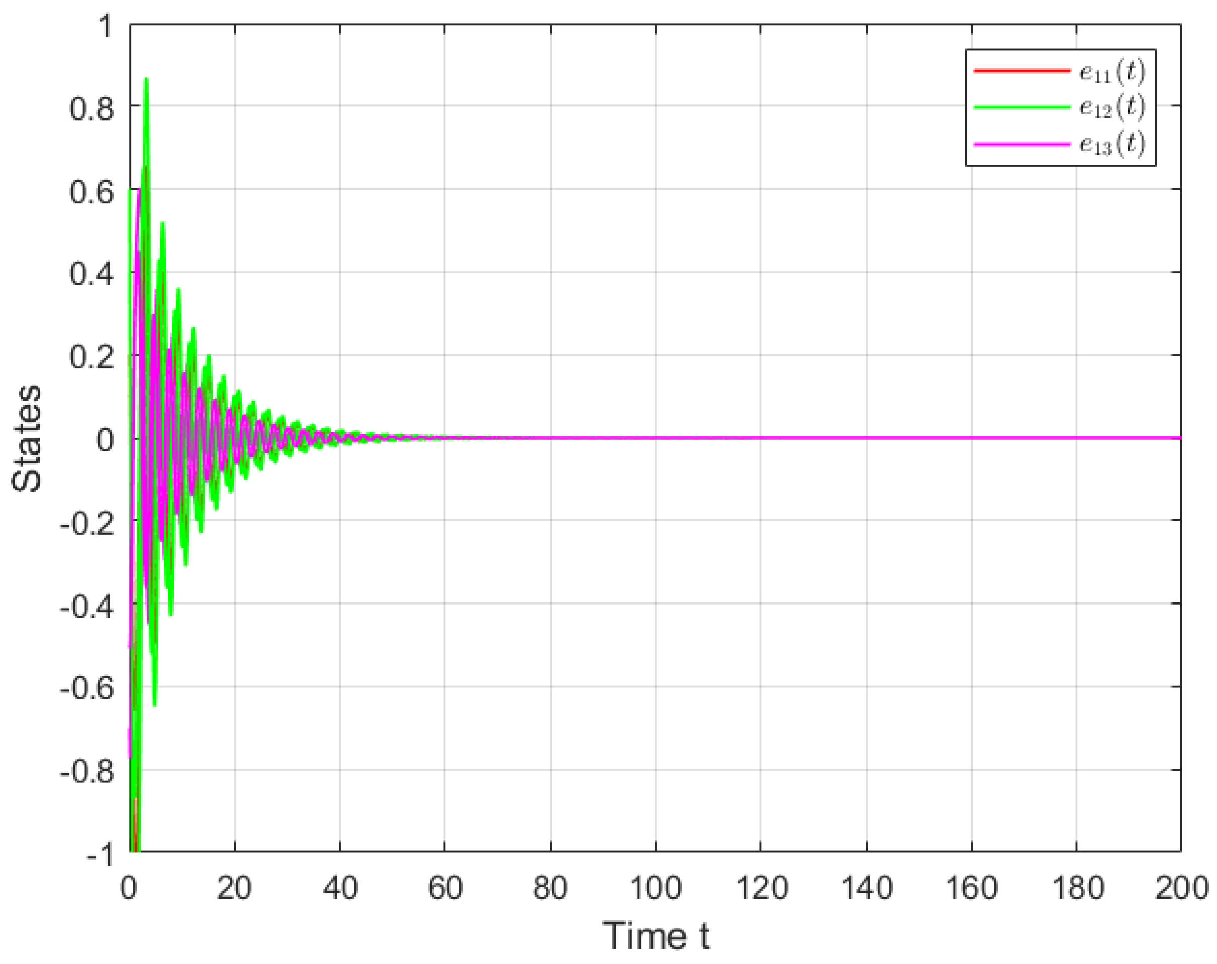
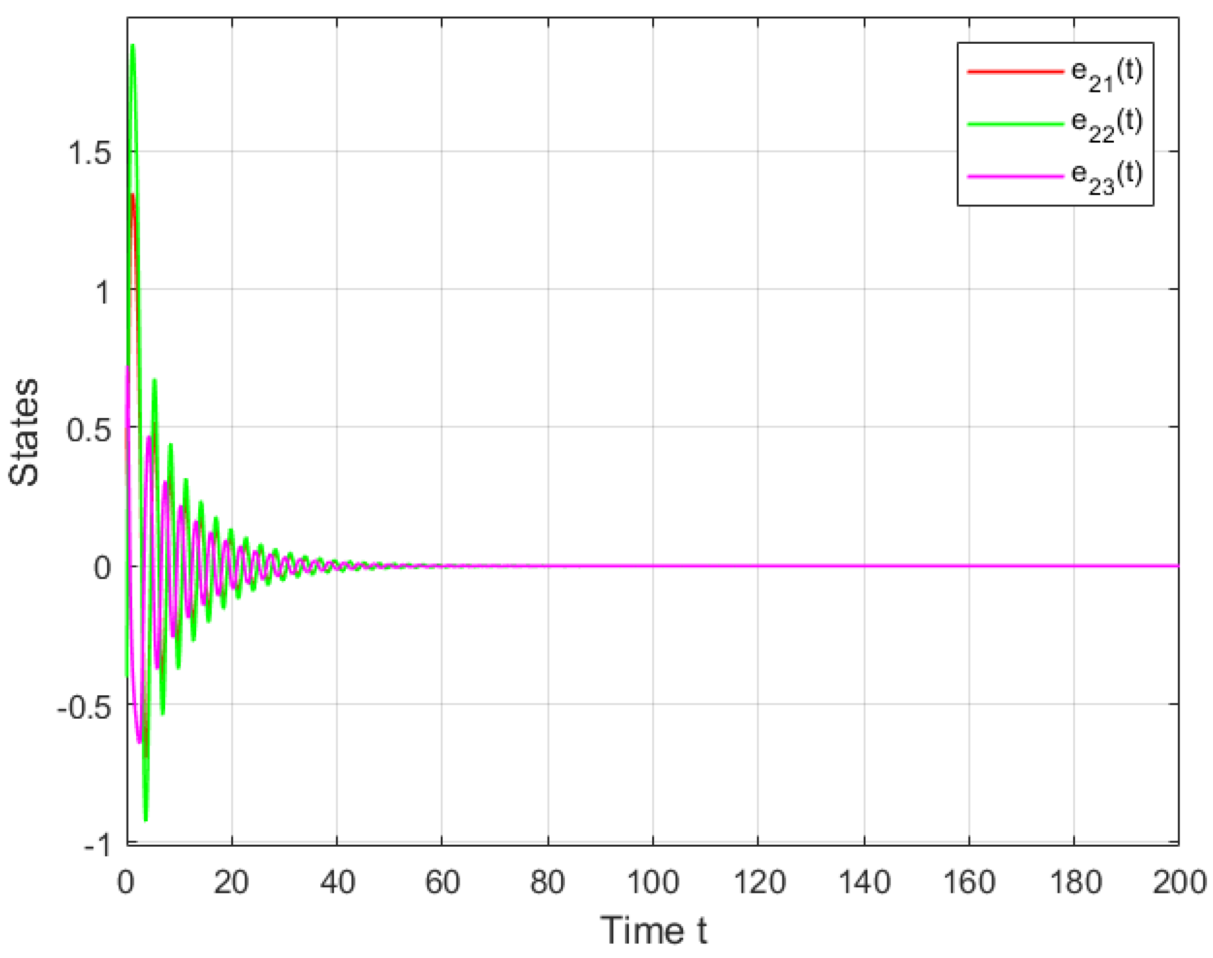
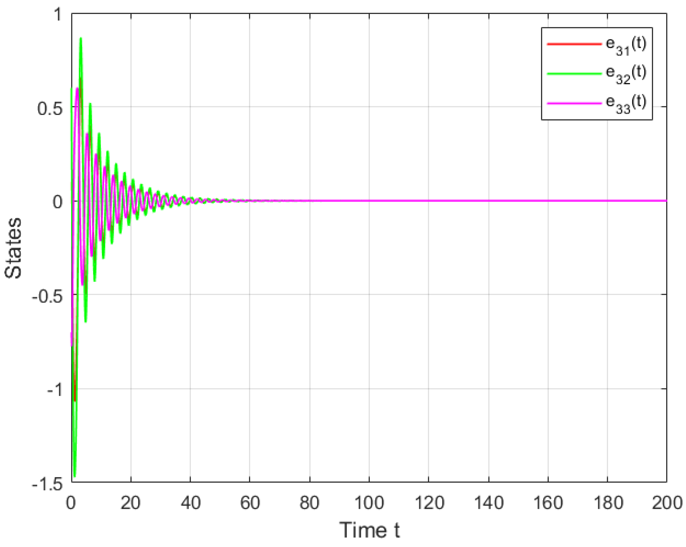
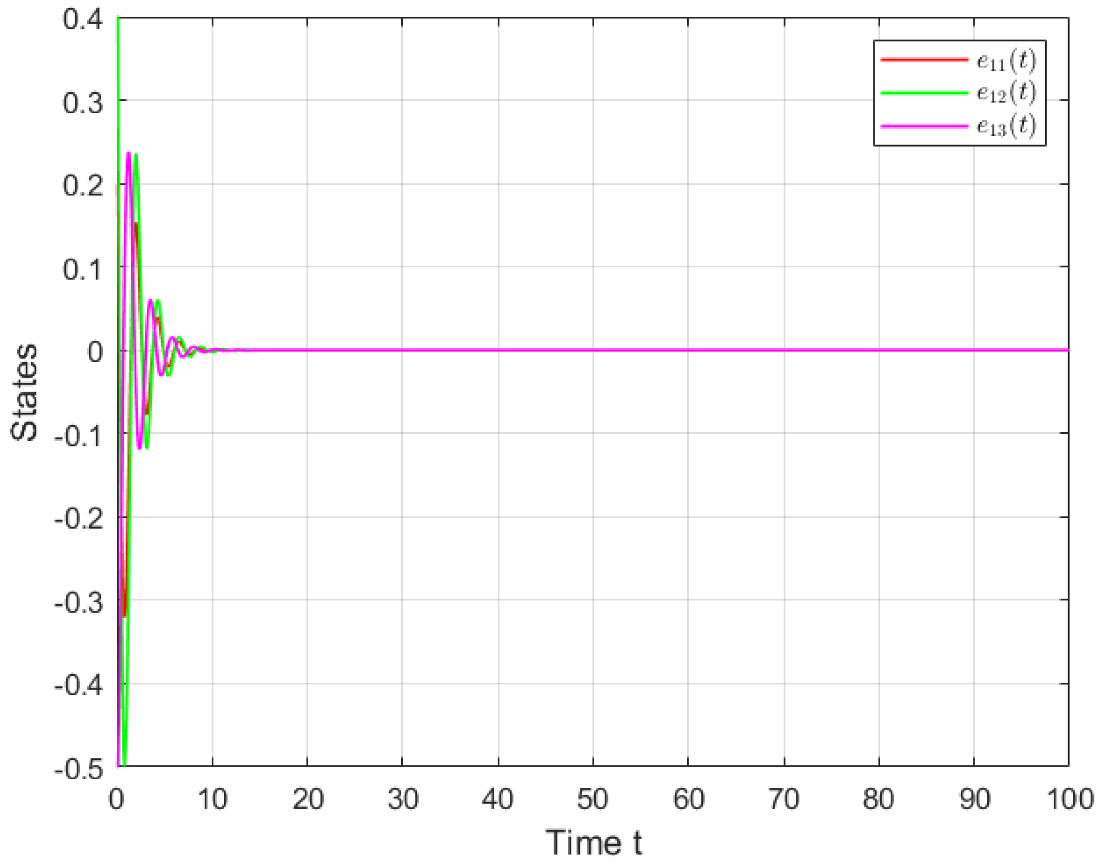
4. Simulations

In this section, two numerical examples are given to illustrate the validity of the theoretical results.

Example 1. 

Consider the following model of CDNs

$$\begin{array}{cc}\hfill {\dot{x}}_p\left(t\right)=& f\left(x_p\left(t\right)\right)+c\sum _{q=1}^3(a_{pq}+△a_{pq}\left(t\right))x_q\left(t\right)+{\varpi }_p\left(t\right).\hfill \end{array}$$

(29)

CDNs (29) is composed of three nodes, $V=1,2,3$. $x_p\left(t\right)={(x_{p1}\left(t\right),x_{p2}\left(t\right),x_{p3}\left(t\right))}^T$. The activation function is as follows

$$\begin{array}{c}\hfill f(x_P\left(t\right),t)=-\widehat{I}{x}_p\left(t\right)+Tg(x_p\left(t\right),t)\end{array}$$

where $x_p\left(t\right)={(x_{p1}\left(t\right),x_{p2}\left(t\right),x_{p3}\left(t\right))}^T\in {\mathbb{R}}^3$.

$$\begin{array}{cc}\hfill g(x_p\left(t\right),t)=& \left(\right(|x_{p1}\left(t\right)+1|-|x_{p1}\left(t\right)-1\left|\right)/2,\left(\right|x_{p2}\left(t\right)+1|\hfill \\ & -|x_{p2}\left(t\right)-1\left|\right)/2,\left(\right|x_{p13}+1|-|x_{p3}{\left(t\right)-1\left|\right)/2)}^T,\hfill \end{array}$$

where

$$T=\left(\begin{array}{ccc}1.25& -3.2& -3.2\\ -3.2& 1.1& -4.4\\ -3.2& 4.4& 1\end{array}\right).$$

The dynamical equation for the isolated node is

$$\begin{array}{c}\hfill \dot{s}\left(t\right)=f\left(s\left(t\right)\right).\end{array}$$

(30)

Let $x_p=x_p\left(t\right)-s\left(t\right)$, $l_p=1$, $\widehat{I}=1$ Then, the error systems as follow,

$$\begin{array}{c}\hfill {\dot{e}}_p\left(t\right)=f\left(e_p\left(t\right)\right)+c\sum _{q=1}^3(a_{pq}+△a_{pq}\left(t\right))e_q\left(t\right)+{\varpi }_p\left(t\right).\\ \end{array}$$

(31)

In order to achieve ESy between the system (29) and (30), the following feedback controller is designed:

$$\begin{array}{c}\hfill {\varpi }_p\left(t\right)={\varsigma }_p(x_p\left(t\right)-s\left(t\right)),\end{array}$$

(32)

where ${\varsigma }_p=1$. Coupling matrix A are defined as

$$A=B=\left(\begin{array}{ccc}-1& 1& 0\\ 1& -1& 0\\ 0& 0& -1\end{array}\right).$$

$$W=\left(\begin{array}{ccc}1& 0& 0\\ 0& 1& 0\\ 0& 0& 1\end{array}\right).$$

The parameters $△a_{pq}\left(t\right)=0.1cos\left(t\right)$, the coupling strength $c=1$ and $M_{pq}^{\left(1\right)}=0.1$.

Let $T=0.4>ln\left(1\right)/0.5=0.1806$, Solving the transcendental Equation (14) results in $\beth =0.031$. When $|A^{*}|=0.01$, the synchronization errors of CDNs (29) and (30) under the controllers are plotted in Figure 1, Figure 2 and Figure 3.

Example 2. 

Consider the following model of CDNs,

$$\begin{array}{cc}\hfill {\dot{x}}_p\left(t\right)=& f\left(x_p\left(t\right)\right)+c\sum _{q=1}^3(a_{pq}+△a_{pq}\left(t\right))x_q\left(t\right)\hfill \\ \hfill & +c\sum _{q=1}^3{b}_{pq}{x}_q\left(\gamma \left(t\right)\right)+{\varpi }_p\left(t\right),\hfill \end{array}$$

(33)

where $x_p\left(t\right)={(x_{p1}\left(t\right),x_{p2}\left(t\right),x_{p3}\left(t\right))}^T$. The dynamical equation for the isolated node is

$$\begin{array}{c}\hfill \dot{s}\left(t\right)=f\left(s\left(t\right)\right).\end{array}$$

(34)

Then, the error systems as follow,

$$\begin{array}{cc}\hfill {\dot{e}}_p\left(t\right)=& f\left(e_p\left(t\right)\right)+c\sum _{q=1}^3(a_{pq}+△a_{pq}\left(t\right))e_q\left(t\right)\hfill \\ \hfill & +c\sum _{q=1}^3{a}_{pq}{e}_q\left(\gamma \left(t\right)\right)+{\varpi }_p\left(t\right),\hfill \end{array}$$

(35)

where $e_p\left(t\right)={(e_{p1}\left(t\right),e_{p2}\left(t\right),e_{p3}\left(t\right))}^T$.

The Parameters are the same as in Example 1. Setting $\gamma \left(t\right)=t_{k-1}+{\varrho }_k/2$ as $t\in \left(t_{k-1},t_k\right]$, $c=0.1$, ${\varrho }_k=0.01$. The number of iteration is set to be $m=150$. According Theorem 2, we obtain that $\overline{\varrho }=0.021$, $\beth =0.074$. Initial states of CDNs (32) are randomly chosen on interval $[-1,1]$. When $|A^{*}|=0.01$, $\left|\varrho \right|=0.01$, Assumption 4 is satisfied, the synchronization errors of CDNs (32) under the controllers are plotted in Figure 4, Figure 5 and Figure 6.

5. Conclusions

In the paper, we investigate the robustness of synchronisation of complex dynamic networks with deviating arguments and parameter uncertainties. Different from conventional linear matrix inequality and Lyapunov theory, this paper makes use of Grunwall’s inequality to derive upper bounds on the lengths of arguments and the size of the parameters. The results of this paper can be further investigated. To begin with, the theory of synchronised robustness of complex networks of integer order can be extended to fractional order. In addition, for right-hand side discontinuous systems such as memristor-based neural networks and neural networks with discontinuous activation functions, synchronisation robustness has been less discussion.

References

- Zhou, J.; Xiang, L.; Liu, Z. Synchronization in complex delayed dynamical networks with impulsive effects. Physica A 2007, 384, 684–692. [Google Scholar] [CrossRef]
- Yu, W.; Chen, G.; Lü, J. On pinning synchronization of complex dynamical networks. Automatica 2009, 45, 429–435. [Google Scholar] [CrossRef]
- Ali, M.S.; Usha, M.; Orman, Z.; Arik, S. Improved result on state estimation for complex dynamical networks with time varying delays and stochastic sampling via sampled-data control. Neural Netw. 2019, 114, 28–37. [Google Scholar]
- Wang, L.; Sun, Y.-X. Robustness of pinning a general complex dynamical network. Phys. Lett. A 2010, 374, 1699–1703. [Google Scholar] [CrossRef]
- Boccaletti, S.; Latora, V.; Moreno, Y.; Chavez, M.; Hwang, D.-U. Complex networks: Structure and dynamics. Phys. Rep. 2023, 424, 175–308. [Google Scholar] [CrossRef]
- Gao, P.; Wang, Y.; Zhao, J.; Zhang, L.; Peng, Y. Links synchronization control for the complex dynamical network. Neurocomputing 2023, 515, 59–67. [Google Scholar] [CrossRef]
- Weng, T.; Chen, X.; Ren, Z.; Xu, J.; Yang, H. Multiple moving agents on complex networks: From intermittent synchronization to complete synchronization. Physica A 2023, 614, 128562. [Google Scholar] [CrossRef]
- Li, Y.; Zhang, J.; Lu, J.; Lou, J. Finite-time synchronization of complex networks with partial communication channels failure. Inf. Sci. 2023, 634, 539–549. [Google Scholar] [CrossRef]
- Li, B. Finite-time synchronization for complex dynamical networks with hybrid coupling and time-varying delay. Nonlinear Dyn. 2014, 76, 1603–1610. [Google Scholar] [CrossRef]
- Wang, J.; Ru, T.; Xia, J.; Wei, Y.; Wang, Z. Finite-time synchronization for complex dynamic networks with semi-markov switching topologies: An h∞ event-triggered control scheme. Appl. Math. Comput. 2019, 356, 235–251. [Google Scholar] [CrossRef]
- Shi, L.; Zhu, H.; Zhong, S.; Zeng, Y.; Cheng, J. Synchronization for time-varying complex networks based on control. J. Comput. Appl. Math. 2016, 301, 178–187. [Google Scholar] [CrossRef]
- Arbi, A.; Cao, J.; Alsaedi, A. Improved synchronization analysis of competitive neural networks with time-varying delays. Nonlinear Anal. Model. 2018, 23, 82–107. [Google Scholar] [CrossRef]
- Liu, X.; Yu, X.; Xi, H. Finite-time synchronization of neutral complex networks with markovian switching based on pinning controller. Neurocomputing 2015, 153, 148–158. [Google Scholar] [CrossRef]
- Xu, Z.; Li, X.; Duan, P. Synchronization of complex networks with time-varying delay of unknown bound via delayed impulsive control. Neural Netw. 2020, 125, 224–232. [Google Scholar] [CrossRef]
- Wu, Y.; Shen, B.; Ahn, C.K.; Li, W. Intermittent dynamic event-triggered control for synchronization of stochastic complex networks. IEEE Trans. Circuits Syst. I Regul. Pap. 2021, 68, 2639–2650. [Google Scholar] [CrossRef]
- Zhu, Q.; Cao, J. Stability analysis of markovian jump stochastic bam neural networks with impulse control and mixed time delays. IEEE Trans. Neural Netw. Learn. Syst. 2012, 23, 467–479. [Google Scholar]
- Akhmet, M.U.; Aruğaslan, D.; Yılmaz, E. Stability analysis of recurrent neural networks with piecewise constant argument of generalized type. Neural Netw. 2010, 23, 805–811. [Google Scholar] [CrossRef] [PubMed]
- Wu, A.; Liu, L.; Huang, T.; Zeng, Z. Mittag-leffler stability of fractional-order neural networks in the presence of generalized piecewise constant arguments. Neural Netw. 2017, 85, 118–127. [Google Scholar] [CrossRef] [PubMed]
- Shen, W.; Zeng, Z.; Wen, S. Synchronization of complex dynamical network with piecewise constant argument of generalized type. Neurocomputing 2016, 173, 671–675. [Google Scholar] [CrossRef]
- Fang, W.; Xie, T.; Li, B. Robustness analysis of fuzzy cellular neural network with deviating argument and stochastic disturbances. IEEE Access 2023, 11, 3717–3728. [Google Scholar]
- Fang, W.; Xie, T.; Li, B. Robustness analysis of bam cellular neural network with deviating arguments of generalized type. Discret. Dyn. Nat. Soc. 2023, 2023, 9570805. [Google Scholar] [CrossRef]
- Zhu, S.; Shen, Y. Robustness analysis for connection weight matrix of global exponential stability recurrent neural networks. Neurocomputing 2013, 101, 370–374. [Google Scholar] [CrossRef]
- Liu, S.; Yu, Y.; Zhang, S. Robust synchronization of memristor-based fractional-order hopfield neural networks with parameter uncertainties. Neural Comput. Appl. 2019, 31, 3533–3542. [Google Scholar] [CrossRef]
- Wong, W.K.; Li, H.; Leung, S. Robust synchronization of fractional-order complex dynamical networks with parametric uncertainties. Commun. Nonlinear Sci. Numer. Simul. 2012, 17, 4877–4890. [Google Scholar] [CrossRef]
- Arbi, A. Robust model predictive control for fractional-order descriptor systems with uncertainty. Fract. Calc. Appl. Anal. 2023, 1–17. [Google Scholar] [CrossRef]
- Zeng, Z.; Wang, J.; Liao, X. Global exponential stability of a general class of recurrent neural networks with time-varying delays. IEEE Trans. Circuits Syst. 2003, 50, 1353–1358. [Google Scholar] [CrossRef]
- Bellman, R. The stability of solutions of linear differential equations. Duke Math. J. 1943, 10, 643–647. [Google Scholar] [CrossRef]
Disclaimer/Publisher’s Note: The statements, opinions and data contained in all publications are solely those of the individual author(s) and contributor(s) and not of MDPI and/or the editor(s). MDPI and/or the editor(s) disclaim responsibility for any injury to people or property resulting from any ideas, methods, instructions or products referred to in the content. |
© 2024 by the authors. Licensee MDPI, Basel, Switzerland. This article is an open access article distributed under the terms and conditions of the Creative Commons Attribution (CC BY) license (https://creativecommons.org/licenses/by/4.0/).
Share and Cite
Xie, T.; Xiong, X. Robustness Analysis of Exponential Synchronization in Complex Dynamic Networks with Deviating Argumentsand Parameter Uncertainties. Symmetry 2024, 16, 158. https://doi.org/10.3390/sym16020158
Xie T, Xiong X. Robustness Analysis of Exponential Synchronization in Complex Dynamic Networks with Deviating Argumentsand Parameter Uncertainties. Symmetry. 2024; 16(2):158. https://doi.org/10.3390/sym16020158
Chicago/Turabian StyleXie, Tao, and Xing Xiong. 2024. "Robustness Analysis of Exponential Synchronization in Complex Dynamic Networks with Deviating Argumentsand Parameter Uncertainties" Symmetry 16, no. 2: 158. https://doi.org/10.3390/sym16020158