A New Test Statistic to Assess the Goodness of Fit of Location-Scale Distribution Based on Progressive Censored Data

Abstract

The problem of examining how well the data fit a supposed distribution is very important, and it must be confirmed prior to any data analysis, because many data analysis methods assume a specific distribution of data. For this purpose, histograms or Q-Q plots are employed for the assessment of data distribution. Additionally, a GoF TstS utilizes distance measurements between the empirical distribution function and the theoretical cumulative distribution function (cdf) to evaluate data distribution. In life-testing or reliability studies, the observed failure time of test units may not be recorded in some situations. The GoF TstSs for completely observed data can no longer be used in progressive type II censored data (PrCsD). In this paper, we suggest a GoF TstSs and new plot method for the GoF test of symmetric and asymmetric location-scale distribution (LoScD) based on PrCsD. The power of the suggested TstSs is estimated through Monte Carlo (MC) simulations, and it is compared with that of the TstSs using the order statistics (OrSt). Furthermore, we analyzed real data examples (symmetric and asymmetric data).

1. Introduction

The problem of examining how well the data fit a supposed distribution is very important, and it must be confirmed prior to any data analysis, because many data analysis methods assume a specific distribution of data. The evaluation of the GoF TstS for a statistical model involves assessing how effectively it aligns with a given set of observations. Measures quantifying GoF typically synthesize the disparities between observed values and those anticipated under the model that is being considered. Usually, histograms or Q-Q plots are employed for the assessment of data distribution. Additionally, a GoF TstS utilizes distance measurements between the empirical distribution function and the theoretical cumulative distribution function (cdf) to evaluate data distribution. In this situation, we reject the null hypothesized distribution if the distance is far in some cases.

In life-testing or reliability studies, the observed failure time of test units may not be recorded in some situations. Furthermore, there are situations wherein the removal of units prior to failure is pre-planned in order to reduce the cost or time associated with testing. Among the censoring methods, progressive Type II censoring schemes (PrCs) have become quite popular in life-testing or reliability studies. The PrCs arises in life-testing or reliability studies as follows. Randomly, $R_1$ surviving test units are removed from the test after observed the 1st failure unit. Moreover, randomly, $R_2$ surviving test units are removed from the test after the observed 2nd failure unit. Finally, all the remaining test units ($R_m=n-R_1-\cdots -R_{m-1}-m$) are removed from the test after the observed mth failure unit. In PrCs, we suppose that integer m and $R=(R_1,R_2,\cdots ,R_m)$ are pre-assigned. Moreover, the ordered observed times for failure units ($X_{1:m:n},\cdots ,X_{m:m:n}$) are referred to as PrCsD (Ref. [1]). Recently, some studies on PrCs were carried out by many authors (Refs. [2,3,4,5,6,7]). Ref. [2] discussed the estimation of reliability in a multi-component stress–strength model for a general class of inverted exponentiated distributions under PrCs. Ref. [3] discussed classical and Bayesian estimation of the inverse Weibull distribution using PrCs. Ref. [4] discussed applying transformer insulation using Weibull extended distribution based on PrCs. Ref. [5] discussed inference on maintenance service policy under step-stress partially accelerated life tests using PrCs. Ref. [6] discussed monitoring the Weibull shape parameter (ShPm) under PrCs in presence of independent competing risks. Ref. [7] discussed the analysis of gamma distribution under PrCs.

The GoF TstSs for completely observed data can no longer be used in PrCsD. For this reason, the GoF test based on PrCsD has received attention from authors (Refs. [8,9,10,11,12,13,14,15,16,17]). Ref. [8] proposed a GoF test for the exponential distribution (ExpD) based on PrCsD using spacings for PrCsD. Ref. [9] proposed approximate GoF tests for LoScD based on PrCsD using empirical distribution function. Ref. [10] proposed GoF tests for LoScD based on PrCsD using spacings for PrCsD. Recently, in Ref. [11], Lee and Lee (2019) proposed a GoF tests and plot method for LoScD based on PrCsD using generalized LrCv. Ref. [12] proposed a GoF test for inverse Rayleigh distribution based on PrCsD using entropy. Ref. [13] proposed a GoF test based on the Gini index of spacings for PrCsD. Ref. [14] proposed a GoF test for ExpD based on general PrScD using spacings for PrCsD. Ref. [15] proposed a GoF test for inverse Weibull distribution based on PrScD using OrSt. Ref. [16] proposed a GoF test for distribution based on type I left censored data. Ref. [17] proposed a GoF test for Rayleigh distribution based on censored data.

While numerous GoF TstS under PrCsD have been proposed in the literature for various distributions, to the best of our knowledge, these tests do not encompass both the TstS and graphical methods. This motivates us to develop new GoF TstS and graphical methods for LoScD for PrCsD. In this paper, therefore, we suggest a GoF TstSs and new graphical method for the GoF test of LoScD based on PrCsD. The rest of this paper is organized as follows. The introduction of the LrCv is presented in Section 2. In Section 3, we propose a GoF TstSs and a new plot method for the GoF test that uses a LrCv. In Section 4, the power of the suggested TstSs is estimated through MC simulations, and it is compared with that of the TstSs proposed by Ref. [10]. In Section 5, we analyze two examples (real data sets). Finally, in Section 6, we present the conclusion.

2. Lorenz Curve

LrCv presents the means to evaluate income disparity between two countries. From the LrCv, Ref. [18] gave terms under which such an LrCv inequality comparison has normative significance. In the case of an increasing and strict concave utility function, Ref. [18] indicates that one prefer a distribution with dominating LrCvs do not cross. Ref. [19] presented an alternative definition of the LrCv in terms of the inverse of continuous variables as well as discrete variables. Let F denote the cdf of income distribution, and the income is assumed to be non-negative. Furthermore, for a given percentile p, let

$$F^{-1}\left(p\right)=\underset{y}{inf}\left\{y\right|F\left(y\right)\ge p\},0\le p\le 1$$

denote the inverse cdf. We suppose throughout that F is a continuous cdf with finite support. Then, the LrCvs corresponding to the distributions with F is defined as

$$L\left(p\right)=\frac{1}{\theta }{\int }_0^{F^{-1}\left(p\right)}ydF\left(y\right),$$

where $\theta$ means the mean of the distribution. Assume that $Y_1,Y_2,\dots ,Y_n$ are positive random variables (RanV) with OrSt $Y_{1:n},Y_{2:n},\dots ,Y_{n:n}$. Then, the sample LrCv (Ref. [20]) is defined by

$$\widehat{L}\left(\frac{i}{n}\right)=\frac{{\sum }_{i=1}^j{Y}_{i:n}}{{\sum }_{i=1}^n{Y}_{i:n}},i=1,2,\dots ,n.$$

Given that the LrCv possesses the property of comparing the degree of wealth distribution between two different distributions, our intention is to utilize it in the development of a goodness-of-fit test statistic.

3. Test Statistics

Let $Y_{1:m:n}<Y_{2:m:n}<\dots <Y_{m:m:n}$ be the PrCsD with PrCs $\mathit{R}=(R_1,R_2,\dots ,R_m)$ from the LoScD. Moreover, let the PrCsD have an LoScD with a probability density function (pdf)

$$f_Y(y;\alpha ,\beta )=\frac{1}{\beta }{f}_X\left(\frac{y-\alpha }{\beta }\right),$$

(1)

where $f_X(·)$ is the known function (Ref. [8]). Furthermore, we assume that location and scale parameters, $\alpha$ and $\beta$, respectively, of $f_Y(y;\alpha ,\beta )$ are unknown and $f_X(·)$ is the standard form of the $f(x;\alpha ,\beta )$. Then, we want to test whether the PrCsD comes from an LoScD with Equation (1), and test the null hypothesis ($H_0$)

$$H_0:F\in F_{\theta }\mathrm{for}\mathrm{some}\theta \in \mathsf{\Theta }=\left\{(\alpha ,\beta )\right|-\infty <\alpha <\infty ,\beta >0\},$$

(2)

where $F=F_Y(Y_{i:m:n};\alpha ,\beta )$ denotes the distribution function (Ref. [8]).

First of all, we introduced GoF TstS based on the distance between OsSt (Ref. [10]). Let ${\nu }_{j:m:n}=U_{j:m:n}-p_{j:m:n}$. Then, ${\nu }_{j:m:n}$ denotes the deviation between the jth OrSt ($U_{j:m:n}$) and its expected value ($p_{j:m:n}=E\left(U_{j:m:n}\right)$) based on the PrCsD. Here,

$$\begin{array}{c}\hfill p_{j:m:n}=1-\prod _{i=m-j+1}^m\left\{\frac{i+R_{m-i+1}+\cdots +R_m}{i+1+R_{m-i+1}+\cdots +R_m}\right\}.\end{array}$$

Then, TstSs based on the deviation between OrSts are obtained as

$$\begin{array}{c}{T}_{m:n}^{\left(1\right)}=\sum _{j=1}^m\frac{{\nu }_{j:m:n}^2}{m},T_{m:n}^{\left(2\right)}=\sum _{j=1}^m\frac{|{\nu }_{j:m:n}|}{m},C_{m:n}^{+}=\underset{i\le j\le m}{max}{\nu }_{j:m:n},\hfill \\ C_{m:n}^{-}=\underset{i\le j\le m}{max}(-{\nu }_{j:m:n}),K_{m:n}=C_{m:n}^{+}+C_{m:n}^{-},C_{m:n}=max(C_{m:n}^{+},C_{m:n}^{-}).\hfill \end{array}$$

(3)

Here, the above TstSs are related to the modified Kolmogorov–Smirnov TstS.

Now, we propose TstSs by using sample LrCv. All LoScD do not have non-negative support. However, the sample LrCv supposed that Y is a non-negative income. Therefore, in order to solve, all values of the ordered PrCsD were subtracted by the value of the 1st ordered PrCsD. Then, each result was added. Furthermore, a sample LrCv cannot show the property of the shape of distribution. Therefore, in order to solve, the result is added from $1-p_{j:m:n}$. Then, the modified sample LrCv is derived as

$$\begin{array}{c}\hfill mLC\left(p_{j:m:n}\right)=\frac{{\sum }_{i=1}^j\left[Y_{i:m:n}-Y_{1:m:n}\right]}{{\sum }_{i=1}^m\left[Y_{i:m:n}-Y_{1:m:n}\right]}-p_{j:m:n}+1,j=1,2,\dots ,m.\end{array}$$

(4)

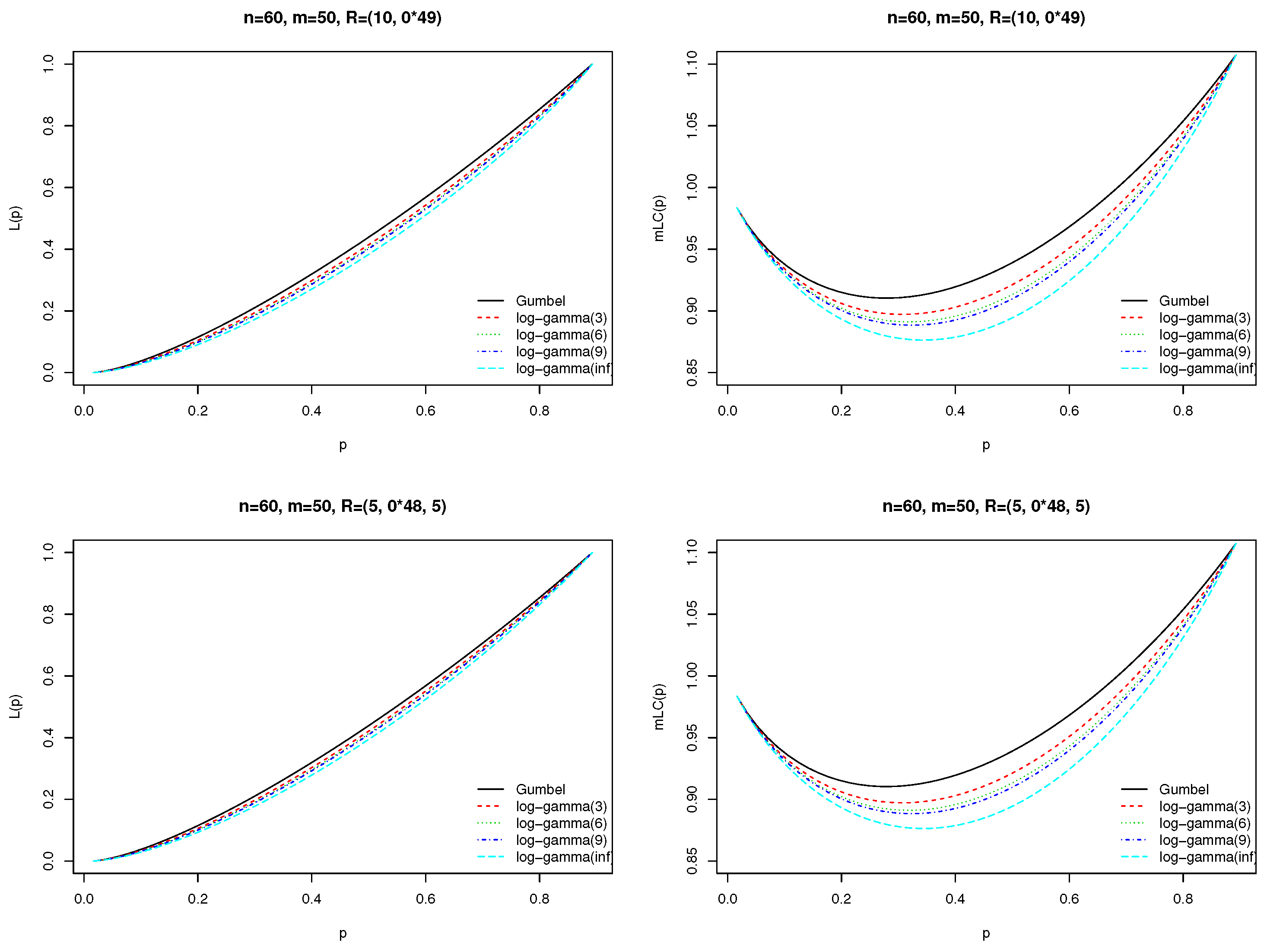
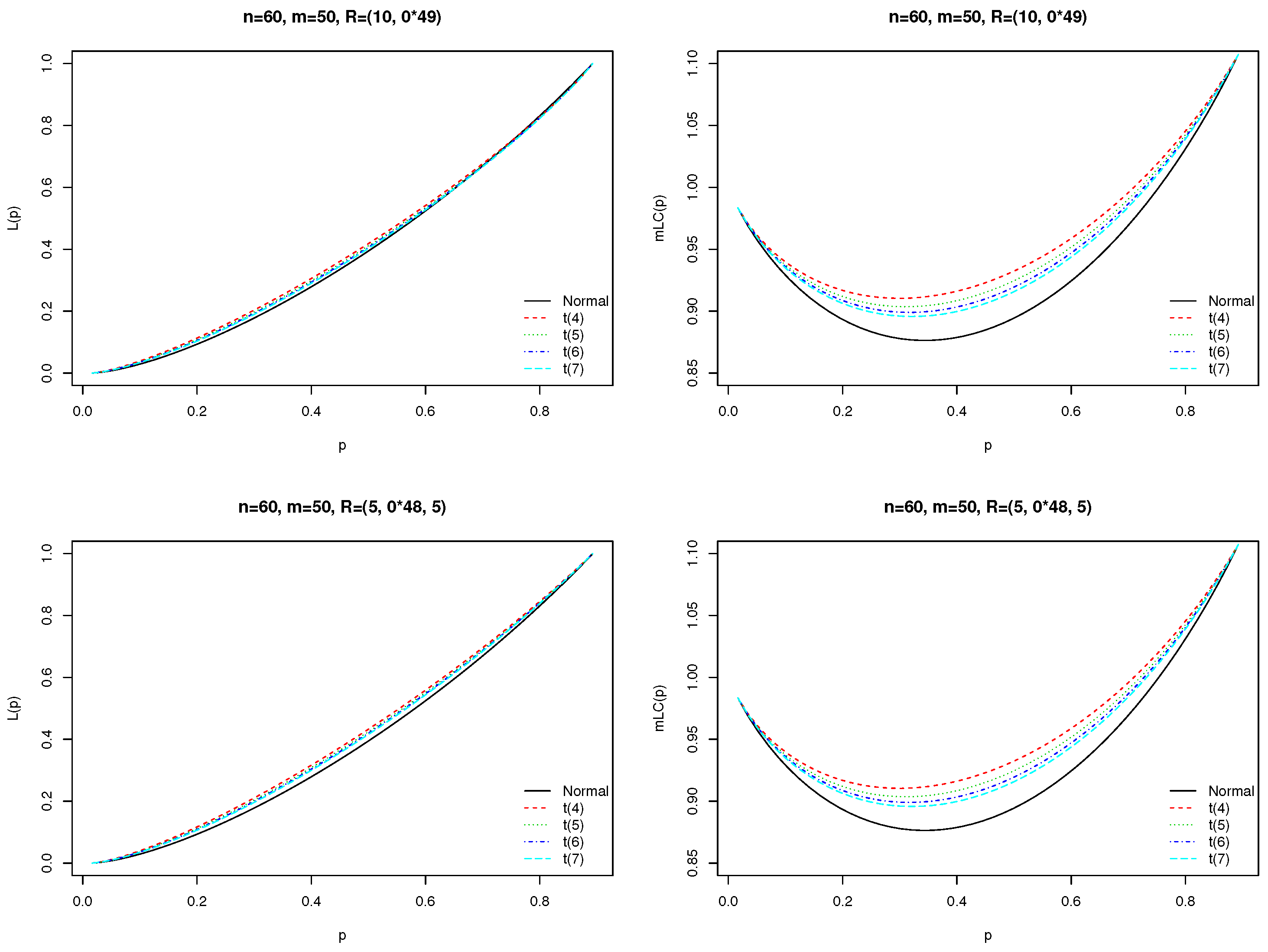
We used the percentile points (%pts) of Gumbel distribution (GumDist), log-gamma distribution (LGamDist) with ShPm 3, 6, 9 and ∞; normal distribution (NormDist); and t distribution (tDist) with 4, 5, 6 and 7 degrees of freedom (DoF) (Figure 1 and Figure 2). As shown in Figure 1 and Figure 2, the modified sample LrCv of LoScDs has a different shape. Here, the modified sample LrCv using the percentile points of LoScD is obtained as

$$\begin{array}{c}\hfill mL{C}_F\left(p_{j:m:n}\right)=\frac{{\sum }_{i=1}^j\left[F_Y^{-1}\left(p_{i:m:n}\right)-F_Y^{-1}\left(p_{1:m:n}\right)\right]}{{\sum }_{i=1}^m\left[F_Y^{-1}\left(p_{i:m:n}\right)-F_Y^{-1}\left(p_{1:m:n}\right)\right]}-p_{j:m:n}+1.\end{array}$$

(5)

Then, the ratio modified sample LrCv using the Equations (4) and (5) is obtained as

$$rLC\left(p_{j:m:n}\right)=\frac{mLC\left(p_{j:m:n}\right)}{mL{C}_F\left(p_{j:m:n}\right)}.$$

(6)

Here, the $rLC\left(p_{j:m:n}\right)$ has the following result.

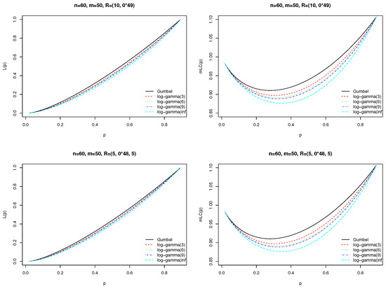
Figure 1. Sample LrCv and modified sample LrCv of GumDist and LGamDist.

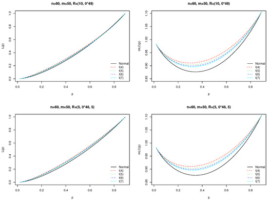
Figure 2. Sample LrCv and modified sample LrCv of NormDist and tDist.

Lemma 1.

$mLC\left(p_{j:m:n}\right)$ and $mL{C}_F\left(p_{j:m:n}\right)$ are a location-scale (LoSc) invariant statistic.

Proof of Lemma 1. 

Let Y be a RanV with a location parameter (LoPm) $\alpha$ and scale parameter (ScPm) $\beta$. Let $X=(Y-\alpha )/\beta$, then $Y=\alpha +\beta X$. The distribution of X does not depend on LoPm $\alpha$ and ScPm $\beta$.

$Y_{i:m:n}-Y_{1:m:n}$ of $mLC\left(p_{j:m:n}\right)$ is

$$\begin{array}{ccc}\hfill Y_{i:m:n}-Y_{1:m:n}& =& (\beta X_{i:m:n}+\alpha )-(\beta X_{1:m:n}+\alpha )\hfill \\ & =& \beta (X_{i:m:n}-X_{1:m:n}).\hfill \end{array}$$

$mLC\left(p_{j:m:n}\right)$ of $rLC\left(p_{j:m:n}\right)$ is

$$\begin{array}{ccc}\hfill mLC\left(p_{j:m:n}\right)& =& \frac{{\sum }_{i=1}^j\left[Y_{i:m:n}-Y_{1:m:n}\right]}{{\sum }_{i=1}^m\left[Y_{i:m:n}-Y_{1:m:n}\right]}-p_{j:m:n}+1\hfill \\ & =& \frac{\beta {\sum }_{i=1}^j\left[X_{i:m:n}-X_{1:m:n}\right]}{\beta {\sum }_{i=1}^m\left[X_{i:m:n}-X_{1:m:n}\right]}-p_{j:m:n}+1\hfill \\ & =& \frac{{\sum }_{i=1}^j\left[X_{i:m:n}-X_{1:m:n}\right]}{{\sum }_{i=1}^m\left[X_{i:m:n}-X_{1:m:n}\right]}-p_{j:m:n}+1.\hfill \end{array}$$

Let $F_Y^{-1}\left(p_{j:m:n}\right)$ have a LoPm $\alpha$ and ScPm $\beta$. If $F_X^{-1}\left(p_{j:m:n}\right)=[F_Y^{-1}\left(p_{j:m:n}\right)-\alpha ]/\beta$, then $F_Y^{-1}\left(p_{j:m:n}\right)=\alpha +\beta F_X^{-1}\left(p_{j:m:n}\right)$. The distribution of $F_X^{-1}\left(p_{j:m:n}\right)$ does not depend on LoPm $\alpha$ and ScPm $\beta$.

$F_Y^{-1}\left(p_{i:m:n}\right)-F_Y^{-1}\left(p_{1:m:n}\right)$ of $mL{C}_F\left(p_{j:m:n}\right)$ is

$$\begin{array}{ccc}\hfill F_Y^{-1}\left(p_{i:m:n}\right)-F_Y^{-1}\left(p_{1:m:n}\right)& =& \left[\beta F_X^{-1}\left(p_{j:m:n}\right)+\alpha \right]-\left[\beta F_X^{-1}\left(p_{1:m:n}\right)+\alpha \right]\hfill \\ & =& \beta \left[F_X^{-1}\left(p_{i:m:n}\right)-F_X^{-1}\left(p_{1:m:n}\right)\right].\hfill \end{array}$$

$mL{C}_F\left(p_{j:m:n}\right)$ of $rLC\left(p_{j:m:n}\right)$ is

$$\begin{array}{ccc}\hfill mL{C}_F\left(p_{j:m:n}\right)& =& \frac{{\sum }_{i=1}^j\left[F_Y^{-1}\left(p_{i:m:n}\right)-F_Y^{-1}\left(p_{1:m:n}\right)\right]}{{\sum }_{i=1}^m\left[F_Y^{-1}\left(p_{i:m:n}\right)-F_Y^{-1}\left(p_{1:m:n}\right)\right]}-p_{j:m:n}+1\hfill \\ & =& \frac{\beta {\sum }_{i=1}^j\left[F_X^{-1}\left(p_{i:m:n}\right)-F_X^{-1}\left(p_{1:m:n}\right)\right]}{\beta {\sum }_{i=1}^m\left[F_X^{-1}\left(p_{i:m:n}\right)-F_X^{-1}\left(p_{1:m:n}\right)\right]}-p_{j:m:n}+1\hfill \\ & =& \frac{{\sum }_{i=1}^j\left[F_X^{-1}\left(p_{i:m:n}\right)-F_X^{-1}\left(p_{1:m:n}\right)\right]}{{\sum }_{i=1}^m\left[F_X^{-1}\left(p_{i:m:n}\right)-F_X^{-1}\left(p_{1:m:n}\right)\right]}-p_{j:m:n}+1.\hfill \end{array}$$

□

Theorem 1.

$rLC\left(p_{j:m:n}\right)$ is a LoSc invariant statistic.

Proof of Theorem 1. 

Theorem 1 is straightforward according to Lemma 1. □

If the data come from an LoScD, we expect all the $rLC\left(p_{j:m:n}\right)$ values to be 1. By applying these properties of $rLC\left(p_{j:m:n}\right)$ to Ref. [10]’s TstSs (Equation (3)), we propose the following TstSs.

$$\begin{array}{c}{L}_{m:n}^{+}=\underset{i\le j\le m}{max}[1-rLC\left(p_{j:m:n}\right)],L_{m:n}^{-}=\underset{i\le j\le m}{max}[-1+rLC\left(p_{j:m:n}\right)],\hfill \\ L_{m:n}^{\left(1\right)}=max(L_{m:n}^{+},L_{m:n}^{-}),L_{m:n}^{\left(2\right)}=L_{m:n}^{+}+L_{m:n}^{-},\hfill \\ L_{m:n}^{\left(3\right)}=\sum _{j=1}^m\frac{{[1-rLC\left(p_{j:m:n}\right)]}^2}{m},L_{m:n}^{\left(4\right)}=\sum _{j=1}^m\frac{|1-rLC(p_{j:m:n}\left)\right|}{m}.\hfill \end{array}$$

(7)

If the data come from an LoScD, we expect $L_{m:n}^{+}$, $L_{m:n}^{-}$, $L_{m:n}^{\left(1\right)}$, $L_{m:n}^{\left(2\right)}$, $L_{m:n}^{\left(3\right)}$ and $L_{m:n}^{\left(4\right)}$ TstSts to be 0. Consequently, large values of $L_{m:n}^{+}$, $L_{m:n}^{-}$, $L_{m:n}^{\left(1\right)}$, $L_{m:n}^{\left(2\right)}$, $L_{m:n}^{\left(3\right)}$ and $L_{m:n}^{\left(4\right)}$ TstSts lead to the rejection of $H_0$ (Equation (2)). Therefore, we reject $H_0$ if $L_{m:n}^{+}$, $L_{m:n}^{-}$, $L_{m:n}^{\left(1\right)}$, $L_{m:n}^{\left(2\right)}$, $L_{m:n}^{\left(3\right)}$ and $L_{m:n}^{\left(4\right)}$ TstSs exceed the corresponding null critical values (CrVal). Since $L_{m:n}^{+}$, $L_{m:n}^{-}$, $L_{m:n}^{\left(1\right)}$, $L_{m:n}^{\left(2\right)}$, $L_{m:n}^{\left(3\right)}$ and $L_{m:n}^{\left(4\right)}$ TstSs have a drawback in that their distribution theory is difficult, the %pts need to be determined through MC simulations because the CrVal are not available explicitly.

Furthermore, using $rLC\left(p_{j:m:n}\right)$, we propose a new plot method for the GoF test. If the data come from an LoScD, we expect all the $rLC\left(p_{j:m:n}\right)$ values to be 1. Therefore, using these property of $rLC\left(p_{j:m:n}\right)$, we would like to propose a new plot method as follows.

$$L-plot\left(p_{j:m:n}\right)=|1-rLC\left(p_{j:m:n}\right)|.$$

(8)

If the data come from an LoScD, the $rLC\left(p_{j:m:n}\right)$ is 1 and $L-plot\left(p_{j:m:n}\right)$ converges with $rLC\left(p_{j:m:n}\right)=0$. Therefore, we are going to test if the data follow the LoScD by using the degree of how much the $L-plot\left(p_{j:m:n}\right)$ is apart from the $rLC\left(p_{j:m:n}\right)=0$.

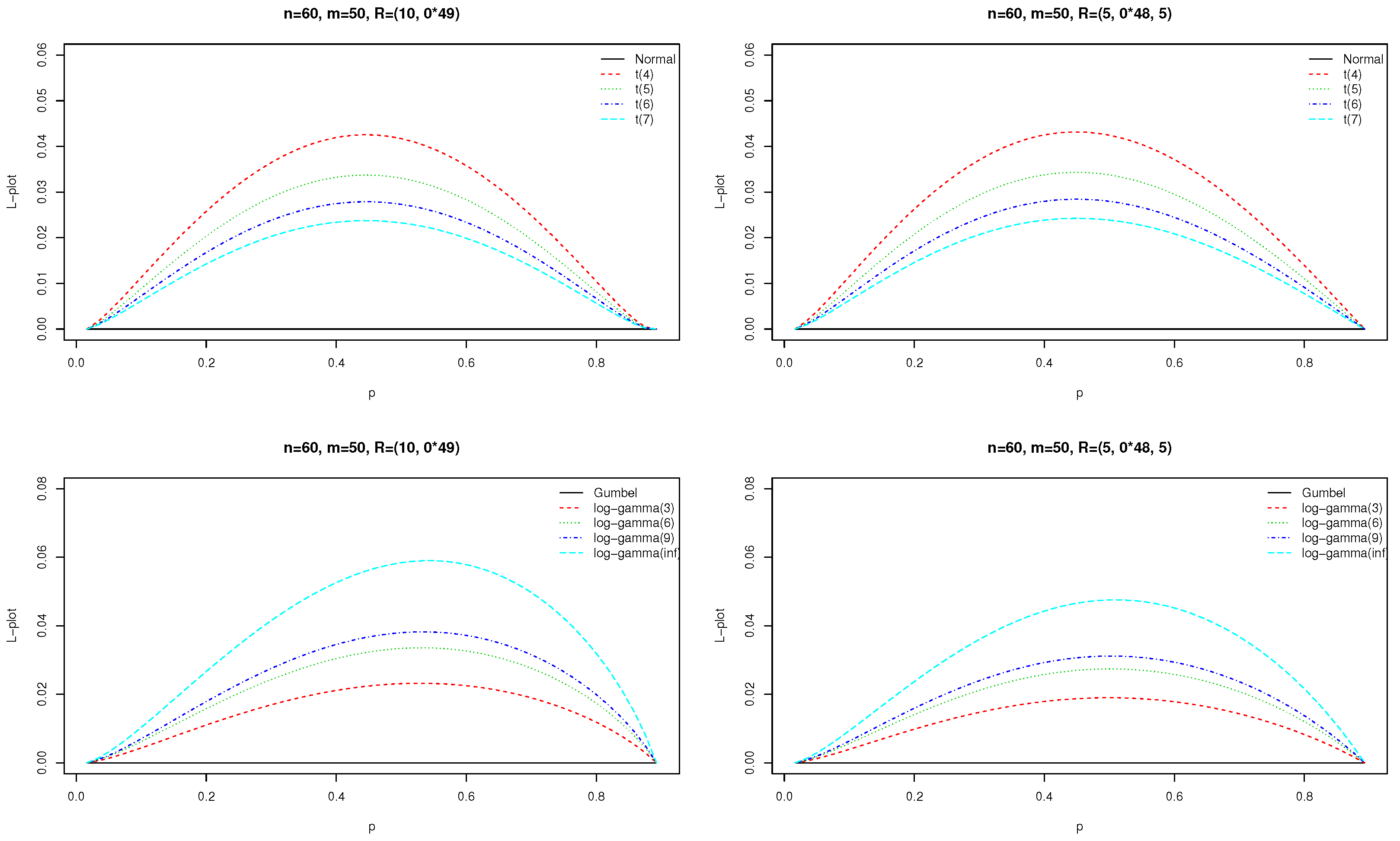
To check the shape of $L-plot\left(p_{j:m:n}\right)$ of various LoScDs, we generate %pts of NormDist; tDist with 4, 5, 6 and 7 DoF; GumDist; and LGamDist with parameter 3, 6, 9 and ∞. Furthermore, we draw the $L-plot\left(p_{j:m:n}\right)$. The results of $L-plot\left(p_{j:m:n}\right)$ for various LoScDs appear in Figure 3. From Figure 3, $L-plot\left(p_{j:m:n}\right)$ converges with the $rLC\left(p_{j:m:n}\right)=0$ at NormDist and GumDist. In tDist and LGamDist, however, $L-plot\left(p_{j:m:n}\right)$ is apart from the x-axis.

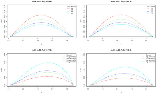
Figure 3. $L-plot\left(p_{j:m:n}\right)$ of various LoScDs.

4. Simulation Result

In this Section, we assess the power of the proposed TstS by comparing the simulated power values with those of Ref. [10]’s TstSs. First of all, we generated 10,000 data for various PrCs (different choices of sample size and PrCs). Here, PrCs were used by Ref. [21].

The proposed TstS is designed to be free of LoSc parameters, ensuring that distributions with these parameters remain unaffected by their specific values. Consequently, the standard distribution serves as the parameter value for the null distribution, ensuring that the power of the test remains consistent irrespective of the parameter value in the null distribution. The alternative distribution, on the other hand, incorporates an ShPm with diverse values to represent a range of distribution shapes.

We consider a NormDist and GumDist as the NuDist. For testing the NormDist, the alternative distribution is considered tDist with 4, 5, 6 and 7 DoF. For testing the GumDist, the alternative distribution is considered LGamDist with ShPm 3, 6, 9 and ∞. All numerical computations are carried out via R 4.3.2 software (Supplementary Materials) utilizing two packages, namely: ‘goftest’ and ‘VGAM’ packages.

When considering the alternative distribution as the distribution from which the data are simulated, the rejection probabilities provide insights into the power of the TstSs. A power value approaching 1 indicates higher test effectiveness. The estimated power are presented in Table 1 and Table 2. The proposed TstSs gained better power as the PrCsD size increased. Table 1 presents the estimated power of the TstSs when the $H_0$ stipulates NormDist and the $H_1$ corresponds to tDist with 4, 5, 6 and 7 DoF. Table 1 shows that the $L_{m:n}^{-}$ TstS possessed better power than Ref. [10]’s TstSs in a number of PrCs (indicated in bold). The $L_{m:n}^{-}$ TstS was found to be better than Ref. [10]’s TstSs in all PrCs. When the data were generated from tDist with 4 DoF, the proposed TstSs gained better power. The $L_{m:n}^{-}$ TstS was always more powerful than the other proposed TstSs. Furthermore, $L_{m:n}^{+}$, $L_{m:n}^{-}$, $L_{m:n}^{\left(1\right)}$, $L_{m:n}^{\left(2\right)}$, $L_{m:n}^{\left(3\right)}$ and $L_{m:n}^{\left(4\right)}$ TstSs were compared with $C_{m:n}^{+}$, $C_{m:n}^{-}$, $C_{m:n}$, $K_{m:n}$, $T_{m:n}^{\left(1\right)}$ and $T_{m:n}^{\left(2\right)}$ TstSs, respectively. As a result, $L_{m:n}^{\left(1\right)}$, $L_{m:n}^{\left(2\right)}$, $L_{m:n}^{\left(3\right)}$ and $L_{m:n}^{\left(4\right)}$ TstSs were found to be better than $C_{m:n}$, $K_{m:n}$, $T_{m:n}^{\left(1\right)}$ and $T_{m:n}^{\left(2\right)}$ TstS in 64, 80, 68 and 68 out of 108 PrCs, respectively.

Table 1. Estimated power values for tDist with 4, 5, 6, and 7 DoF when $H_0$ is the NormDist.

Sch.No.	df	${\mathit{L}}_{\mathit{m}:\mathit{n}}^{+}$	${\mathit{L}}_{\mathit{m}:\mathit{n}}^{-}$	${\mathit{L}}_{\mathit{m}:\mathit{n}}^{\left(1\right)}$	${\mathit{L}}_{\mathit{m}:\mathit{n}}^{\left(2\right)}$	${\mathit{L}}_{\mathit{m}:\mathit{n}}^{\left(3\right)}$	${\mathit{L}}_{\mathit{m}:\mathit{n}}^{\left(4\right)}$	${\mathit{C}}_{\mathit{m}:\mathit{n}}^{+}$	${\mathit{C}}_{\mathit{m}:\mathit{n}}^{-}$	${\mathit{C}}_{\mathit{m}:\mathit{n}}$	${\mathit{K}}_{\mathit{m}:\mathit{n}}$	${\mathit{T}}_{\mathit{m}:\mathit{n}}^{\left(1\right)}$	${\mathit{T}}_{\mathit{m}:\mathit{n}}^{\left(2\right)}$
1	4	0.0458	0.1457	0.0489	0.0495	0.0609	0.0656	0.1186	0.0557	0.1172	0.0746	0.1223	0.1129
	5	0.0449	0.1202	0.0460	0.0460	0.0539	0.0567	0.0990	0.0509	0.0961	0.0622	0.0973	0.0911
	6	0.0443	0.1049	0.0456	0.0460	0.0512	0.0536	0.0877	0.0488	0.0819	0.0557	0.0842	0.0787
	7	0.0441	0.0947	0.0451	0.0454	0.0501	0.0532	0.0789	0.0484	0.0759	0.0514	0.0761	0.0719
2	4	0.0363	0.1399	0.0380	0.0383	0.0542	0.0600	0.1144	0.0357	0.0706	0.0688	0.0725	0.0786
	5	0.0349	0.1180	0.0372	0.0376	0.0491	0.0546	0.0958	0.0338	0.0608	0.0606	0.0606	0.0681
	6	0.0329	0.1046	0.0363	0.0366	0.0472	0.0507	0.0862	0.0309	0.0533	0.0566	0.0563	0.0603
	7	0.0295	0.0961	0.0359	0.0363	0.0470	0.0486	0.0787	0.0287	0.0521	0.0547	0.0547	0.0573
3	4	0.0354	0.1497	0.0363	0.0365	0.0475	0.0552	0.1314	0.0351	0.1017	0.0639	0.0991	0.0987
	5	0.0336	0.1257	0.0350	0.0353	0.0437	0.0483	0.1084	0.0332	0.0848	0.0547	0.0807	0.0826
	6	0.0305	0.1096	0.0325	0.0328	0.0434	0.0456	0.0964	0.0306	0.0753	0.0511	0.0709	0.0718
	7	0.0281	0.0995	0.0321	0.0324	0.0425	0.0452	0.0876	0.0281	0.0695	0.0495	0.0642	0.0657
4	4	0.0523	0.1774	0.0923	0.0953	0.1106	0.1169	0.1294	0.0727	0.1329	0.0982	0.1389	0.1346
	5	0.0478	0.1466	0.0746	0.0764	0.0898	0.0934	0.1051	0.0624	0.1049	0.0778	0.1071	0.1069
	6	0.0464	0.1271	0.0666	0.0668	0.0774	0.0812	0.0911	0.0573	0.0892	0.0651	0.0907	0.0904
	7	0.0455	0.1151	0.0617	0.0624	0.0715	0.0747	0.0814	0.0552	0.0812	0.0601	0.0806	0.0808
5	4	0.0340	0.1844	0.0784	0.0783	0.1083	0.1130	0.1289	0.0343	0.0861	0.0657	0.0870	0.0869
	5	0.0320	0.1530	0.0645	0.0638	0.0859	0.0912	0.1045	0.0323	0.0697	0.0562	0.0721	0.0722
	6	0.0285	0.1327	0.0583	0.0576	0.0745	0.0784	0.0882	0.0287	0.0623	0.0524	0.0637	0.0646
	7	0.0252	0.1176	0.0541	0.0539	0.0688	0.0708	0.0797	0.0260	0.0577	0.0504	0.0591	0.0610
6	4	0.0449	0.1993	0.1064	0.1086	0.1291	0.1346	0.0425	0.1129	0.0823	0.0897	0.0992	0.1059
	5	0.0433	0.1644	0.0838	0.0853	0.1091	0.1110	0.0416	0.0925	0.0686	0.0686	0.0806	0.0839
	6	0.0435	0.1414	0.0712	0.0725	0.0905	0.0959	0.0410	0.0810	0.0628	0.0623	0.0695	0.0728
	7	0.0436	0.1255	0.0667	0.0675	0.0798	0.0838	0.0409	0.0746	0.0591	0.0581	0.0635	0.0657
7	4	0.0565	0.1900	0.1311	0.1358	0.1461	0.1486	0.1267	0.0915	0.1470	0.1132	0.1552	0.1522
	5	0.0519	0.1577	0.1016	0.1039	0.1194	0.1221	0.1036	0.0754	0.1154	0.0841	0.1185	0.1189
	6	0.0501	0.1369	0.0883	0.0892	0.1008	0.1053	0.0898	0.0690	0.0956	0.0693	0.0975	0.0967
	7	0.0483	0.1224	0.0778	0.0788	0.0891	0.0918	0.0821	0.0636	0.0837	0.0621	0.0868	0.0850
8	4	0.0343	0.2086	0.1159	0.1161	0.1414	0.1465	0.1302	0.0388	0.0993	0.0784	0.1030	0.1048
	5	0.0316	0.1702	0.0925	0.0925	0.1150	0.1206	0.1056	0.0372	0.0813	0.0631	0.0822	0.0812
	6	0.0296	0.1474	0.0803	0.0799	0.0981	0.1034	0.0919	0.0364	0.0698	0.0555	0.0721	0.0709
	7	0.0262	0.1302	0.0718	0.0716	0.0867	0.0920	0.0823	0.0355	0.0629	0.0516	0.0643	0.0646
9	4	0.0561	0.1972	0.1492	0.1536	0.1591	0.1613	0.0724	0.1090	0.1059	0.0964	0.1254	0.1306
	5	0.0521	0.1622	0.1193	0.1224	0.1300	0.1333	0.0559	0.0871	0.0840	0.0730	0.0938	0.0988
	6	0.0499	0.1406	0.1020	0.1024	0.1133	0.1157	0.0509	0.0760	0.0724	0.0624	0.0779	0.0819
	7	0.0484	0.1267	0.0911	0.0916	0.1016	0.1042	0.0492	0.0693	0.0653	0.0562	0.0691	0.0709
10	4	0.0364	0.2118	0.0476	0.0468	0.0729	0.0804	0.1772	0.0493	0.1645	0.1153	0.1759	0.1644
	5	0.0357	0.1698	0.0404	0.0407	0.0568	0.0631	0.1393	0.0454	0.1280	0.0853	0.1361	0.1264
	6	0.0338	0.1444	0.0397	0.0399	0.0508	0.0552	0.1186	0.0438	0.1057	0.0723	0.1137	0.1037
	7	0.0336	0.1283	0.0390	0.0387	0.0483	0.0518	0.1026	0.0430	0.0941	0.0638	0.0987	0.0907
11	4	0.0346	0.1740	0.0418	0.0416	0.0705	0.0778	0.1570	0.0327	0.0837	0.0814	0.0916	0.0971
	5	0.0320	0.1440	0.0398	0.0398	0.0590	0.0664	0.1299	0.0303	0.0687	0.0663	0.0725	0.0766
	6	0.0297	0.1248	0.0396	0.0396	0.0534	0.0578	0.1105	0.0269	0.0606	0.0606	0.0640	0.0668
	7	0.0262	0.1113	0.0389	0.0391	0.0502	0.0539	0.0999	0.0231	0.0562	0.0559	0.0592	0.0630
12	4	0.0315	0.2116	0.0651	0.0650	0.0972	0.1075	0.0904	0.0297	0.0627	0.0608	0.0851	0.0986
	5	0.0292	0.1761	0.0528	0.0528	0.0767	0.0842	0.0726	0.0272	0.0518	0.0485	0.0682	0.0768
	6	0.0252	0.1523	0.0478	0.0477	0.0658	0.0721	0.0638	0.0247	0.0479	0.0441	0.0592	0.0674
	7	0.0224	0.1338	0.0463	0.0464	0.0599	0.0646	0.0587	0.0228	0.0464	0.0422	0.0535	0.0603
13	4	0.0372	0.2846	0.1677	0.1771	0.1856	0.1862	0.2108	0.0944	0.2155	0.1804	0.2348	0.2314
	5	0.0368	0.2322	0.1267	0.1309	0.1437	0.1442	0.1636	0.0799	0.1618	0.1310	0.1746	0.1713
	6	0.0366	0.1948	0.1043	0.1074	0.1193	0.1198	0.1361	0.0641	0.1289	0.1013	0.1393	0.1388
	7	0.0365	0.1674	0.0898	0.0921	0.1044	0.1060	0.1167	0.0588	0.1119	0.0846	0.1190	0.1166
14	4	0.0257	0.2599	0.1546	0.1557	0.1794	0.1872	0.2017	0.0278	0.1371	0.1082	0.1467	0.1500
	5	0.0233	0.2087	0.1198	0.1208	0.1387	0.1454	0.1537	0.0254	0.1041	0.0824	0.1068	0.1092
	6	0.0207	0.1782	0.1025	0.1028	0.1169	0.1216	0.1285	0.0212	0.0859	0.0706	0.0859	0.0889
	7	0.0157	0.1531	0.0907	0.0903	0.1038	0.1073	0.1106	0.0185	0.0749	0.0629	0.0752	0.0771
15	4	0.0260	0.3064	0.1961	0.1975	0.2150	0.2209	0.0566	0.1620	0.1074	0.1197	0.1412	0.1549
	5	0.0235	0.2454	0.1455	0.1464	0.1658	0.1717	0.0483	0.1213	0.0811	0.0869	0.1022	0.1154
	6	0.0197	0.2071	0.1197	0.1191	0.1364	0.1409	0.0425	0.0993	0.0682	0.0720	0.0799	0.0920
	7	0.0167	0.1777	0.1045	0.1036	0.1180	0.1217	0.0417	0.0862	0.0603	0.0656	0.0708	0.0790
16	4	0.0410	0.3074	0.2301	0.2478	0.2329	0.2313	0.2024	0.1418	0.2252	0.2166	0.2527	0.2561
	5	0.0378	0.2443	0.1772	0.1852	0.1818	0.1825	0.1490	0.1026	0.1636	0.1507	0.1843	0.1858
	6	0.0366	0.2062	0.1452	0.1492	0.1500	0.1510	0.1215	0.0822	0.1304	0.1154	0.1432	0.1442
	7	0.0360	0.1817	0.1245	0.1272	0.1284	0.1306	0.1051	0.0724	0.1094	0.0942	0.1157	0.1161
17	4	0.0218	0.3294	0.2343	0.2376	0.2538	0.2562	0.2040	0.0367	0.1474	0.1271	0.1622	0.1625
	5	0.0196	0.2636	0.1812	0.1817	0.1985	0.1995	0.1518	0.0327	0.1082	0.0910	0.1169	0.1163
	6	0.0166	0.2191	0.1480	0.1488	0.1637	0.1653	0.1210	0.0322	0.0869	0.0725	0.0946	0.0947
	7	0.0140	0.1892	0.1252	0.1261	0.1382	0.1417	0.1064	0.0322	0.0746	0.0648	0.0799	0.0801
18	4	0.0222	0.3367	0.2406	0.2448	0.2567	0.2586	0.2132	0.0515	0.1690	0.1506	0.1853	0.1855
	5	0.0203	0.2686	0.1863	0.1881	0.1985	0.2007	0.1620	0.0413	0.1242	0.1084	0.1337	0.1353
	6	0.0174	0.2218	0.1525	0.1535	0.1639	0.1668	0.1317	0.0382	0.1012	0.0868	0.1071	0.1089
	7	0.0144	0.1920	0.1285	0.1304	0.1374	0.1417	0.1127	0.0382	0.0873	0.0747	0.0908	0.0932
19	4	0.0307	0.3383	0.1828	0.1937	0.2060	0.2050	0.2659	0.0826	0.2604	0.2198	0.2852	0.2784
	5	0.0286	0.2688	0.1328	0.1383	0.1527	0.1532	0.2050	0.0627	0.1943	0.1592	0.2111	0.2063
	6	0.0279	0.2262	0.1056	0.1080	0.1224	0.1238	0.1654	0.0556	0.1542	0.1208	0.1675	0.1650
	7	0.0274	0.1933	0.0899	0.0914	0.1056	0.1064	0.1413	0.0508	0.1292	0.0996	0.1403	0.1385
20	4	0.0252	0.2622	0.1505	0.1528	0.1761	0.1838	0.2376	0.0248	0.1500	0.1277	0.1689	0.1725
	5	0.0226	0.2127	0.1166	0.1179	0.1352	0.1444	0.1786	0.0217	0.1128	0.0946	0.1215	0.1229
	6	0.0205	0.1796	0.1005	0.1011	0.1140	0.1189	0.1465	0.0180	0.0890	0.0814	0.0959	0.0975
	7	0.0156	0.1568	0.0893	0.0896	0.1029	0.1058	0.1266	0.0135	0.0770	0.0715	0.0812	0.0829
21	4	0.0246	0.2865	0.1640	0.1653	0.1921	0.1971	0.2359	0.0272	0.1836	0.1315	0.1945	0.1929
	5	0.0214	0.2313	0.1221	0.1227	0.1445	0.1501	0.1775	0.0244	0.1392	0.0962	0.1456	0.1457
	6	0.0187	0.1952	0.1045	0.1039	0.1200	0.1240	0.1462	0.0225	0.1130	0.0790	0.1164	0.1180
	7	0.0146	0.1698	0.0898	0.0897	0.1085	0.1085	0.1278	0.0210	0.0973	0.0684	0.0986	0.1006
22	4	0.0294	0.3851	0.3064	0.3300	0.3084	0.3016	0.2890	0.1739	0.3061	0.3062	0.3523	0.3584
	5	0.0286	0.3091	0.2322	0.2478	0.2369	0.2336	0.2124	0.1197	0.2147	0.2109	0.2529	0.2573
	6	0.0285	0.2573	0.1894	0.1980	0.1945	0.1918	0.1661	0.0906	0.1661	0.1569	0.1916	0.1965
	7	0.0278	0.2232	0.1597	0.1655	0.1663	0.1659	0.1374	0.0761	0.1361	0.1240	0.1574	0.1585
23	4	0.0178	0.3977	0.3056	0.3103	0.3179	0.3191	0.2790	0.0396	0.2120	0.1805	0.2442	0.2474
	5	0.0145	0.3139	0.2341	0.2389	0.2437	0.2477	0.2054	0.0304	0.1471	0.1189	0.1659	0.1695
	6	0.0123	0.2610	0.1925	0.1944	0.2005	0.2033	0.1604	0.0277	0.1128	0.0903	0.1253	0.1272
	7	0.0082	0.2251	0.1609	0.1631	0.1696	0.1730	0.1356	0.0268	0.0948	0.0757	0.1007	0.1025
24	4	0.0208	0.4136	0.3289	0.3404	0.3385	0.3346	0.1361	0.2345	0.2134	0.2256	0.2603	0.2671
	5	0.0184	0.3317	0.2512	0.2595	0.2603	0.2593	0.0940	0.1693	0.1488	0.1557	0.1772	0.1864
	6	0.0162	0.2750	0.2048	0.2101	0.2117	0.2118	0.0720	0.1308	0.1152	0.1203	0.1303	0.1394
	7	0.0139	0.2356	0.1711	0.1757	0.1810	0.1804	0.0617	0.1107	0.0963	0.0998	0.1078	0.1113
25	4	0.0274	0.3932	0.3307	0.3557	0.3276	0.3200	0.2694	0.2101	0.3014	0.3135	0.3564	0.3658
	5	0.0271	0.3162	0.2550	0.2715	0.2568	0.2511	0.1902	0.1434	0.2093	0.2090	0.2458	0.2530
	6	0.0264	0.2654	0.2060	0.2134	0.2090	0.2064	0.1476	0.1072	0.1554	0.1527	0.1791	0.1866
	7	0.0263	0.2262	0.1778	0.1833	0.1800	0.1773	0.1210	0.0893	0.1251	0.1189	0.1442	0.1492
26	4	0.0180	0.4289	0.3567	0.3589	0.3625	0.3670	0.2566	0.0624	0.2018	0.1859	0.2264	0.2300
	5	0.0154	0.3434	0.2736	0.2759	0.2836	0.2880	0.1821	0.0430	0.1402	0.1254	0.1538	0.1550
	6	0.0115	0.2852	0.2189	0.2204	0.2266	0.2312	0.1427	0.0382	0.1077	0.0945	0.1155	0.1170
	7	0.0073	0.2416	0.1870	0.1876	0.1923	0.1966	0.1193	0.0369	0.0911	0.0771	0.0932	0.0947
27	4	0.0188	0.4307	0.3561	0.3584	0.3636	0.3656	0.2630	0.0862	0.2206	0.2126	0.2530	0.2537
	5	0.0158	0.3453	0.2738	0.2762	0.2830	0.2858	0.1910	0.0607	0.1547	0.1418	0.1740	0.1759
	6	0.0124	0.2882	0.2180	0.2191	0.2260	0.2286	0.1478	0.0498	0.1188	0.1080	0.1313	0.1321
	7	0.0085	0.2423	0.1853	0.1865	0.1931	0.1949	0.1237	0.0460	0.1014	0.0883	0.1074	0.1076

Table 2. Estimated power values for LGamDist with ShPm 3, 6, 9, and ∞ when the $H_0$ is the GumDist.

Sch.No.	df	${\mathit{L}}_{\mathit{m}:\mathit{n}}^{+}$	${\mathit{L}}_{\mathit{m}:\mathit{n}}^{-}$	${\mathit{L}}_{\mathit{m}:\mathit{n}}^{\left(1\right)}$	${\mathit{L}}_{\mathit{m}:\mathit{n}}^{\left(2\right)}$	${\mathit{L}}_{\mathit{m}:\mathit{n}}^{\left(3\right)}$	${\mathit{L}}_{\mathit{m}:\mathit{n}}^{\left(4\right)}$	${\mathit{C}}_{\mathit{m}:\mathit{n}}^{+}$	${\mathit{C}}_{\mathit{m}:\mathit{n}}^{-}$	${\mathit{C}}_{\mathit{m}:\mathit{n}}$	${\mathit{K}}_{\mathit{m}:\mathit{n}}$	${\mathit{T}}_{\mathit{m}:\mathit{n}}^{\left(1\right)}$	${\mathit{T}}_{\mathit{m}:\mathit{n}}^{\left(2\right)}$
1	3	0.0807	0.0060	0.0783	0.0783	0.0789	0.0783	0.0531	0.0559	0.0531	0.0325	0.0573	0.0663
	6	0.0968	0.0117	0.0938	0.0938	0.0952	0.0938	0.0556	0.0663	0.0556	0.0457	0.0579	0.0665
	9	0.1061	0.0134	0.1005	0.1006	0.1048	0.1005	0.0582	0.0686	0.0582	0.0495	0.0618	0.0683
	∞	0.1580	0.0214	0.1430	0.1436	0.1522	0.1430	0.0657	0.0765	0.0657	0.0595	0.0645	0.0814
2	3	0.0601	0.0200	0.0601	0.0598	0.0602	0.0609	0.0608	0.1112	0.0608	0.0764	0.0543	0.0507
	6	0.0649	0.0292	0.0649	0.0646	0.0651	0.0660	0.0688	0.1185	0.0688	0.0812	0.0653	0.0625
	9	0.0668	0.0313	0.0668	0.0667	0.0676	0.0681	0.0711	0.1222	0.0711	0.0824	0.0683	0.0655
	∞	0.0767	0.0376	0.0767	0.0766	0.0783	0.0785	0.0789	0.1359	0.0789	0.0867	0.0776	0.0759
3	3	0.0638	0.0143	0.0638	0.0638	0.0653	0.0666	0.0545	0.0992	0.0545	0.0615	0.0400	0.0357
	6	0.0705	0.0233	0.0705	0.0705	0.0730	0.0732	0.0640	0.0996	0.0640	0.0709	0.0536	0.0500
	9	0.0735	0.0264	0.0735	0.0734	0.0754	0.0760	0.0660	0.1005	0.0660	0.0733	0.0573	0.0540
	∞	0.0890	0.0325	0.0890	0.0890	0.0920	0.0920	0.0734	0.1030	0.0734	0.0801	0.0693	0.0640
4	3	0.0878	0.0024	0.0866	0.0870	0.0855	0.0840	0.0760	0.0378	0.0760	0.0298	0.0954	0.0876
	6	0.1191	0.0082	0.1110	0.1108	0.1108	0.1083	0.0780	0.0528	0.0778	0.0397	0.1011	0.1190
	9	0.1240	0.0108	0.1229	0.1230	0.1223	0.1194	0.0778	0.0572	0.0780	0.0433	0.1047	0.1234
	∞	0.1894	0.0183	0.1876	0.1879	0.1875	0.1839	0.0912	0.0669	0.0917	0.0539	0.1392	0.1708
5	3	0.0673	0.0087	0.0655	0.0658	0.0633	0.0606	0.0524	0.0620	0.0524	0.0477	0.0306	0.0280
	6	0.0779	0.0175	0.0765	0.0767	0.0723	0.0685	0.0637	0.0709	0.0637	0.0583	0.0458	0.0410
	9	0.0824	0.0205	0.0805	0.0807	0.0770	0.0725	0.0664	0.0724	0.0664	0.0618	0.0496	0.0448
	∞	0.1061	0.0285	0.1040	0.1044	0.0975	0.0932	0.0754	0.0784	0.0754	0.0701	0.0617	0.0563
6	3	0.0837	0.0036	0.0784	0.0790	0.0735	0.0727	0.0471	0.0454	0.0471	0.0380	0.0609	0.0779
	6	0.1061	0.0115	0.0990	0.0995	0.0893	0.0900	0.0557	0.0568	0.0557	0.0508	0.0616	0.0809
	9	0.1186	0.0141	0.1102	0.1110	0.1000	0.0984	0.0602	0.0607	0.0602	0.0560	0.0666	0.0815
	∞	0.1779	0.0221	0.1684	0.1699	0.1511	0.1469	0.0690	0.0709	0.0690	0.0663	0.0684	0.1028
7	3	0.0898	0.0062	0.0827	0.0835	0.0818	0.0805	0.0895	0.0272	0.0895	0.0300	0.1133	0.1312
	6	0.1138	0.0081	0.1058	0.1060	0.1031	0.1001	0.0951	0.0429	0.0951	0.0334	0.1305	0.1577
	9	0.1263	0.0115	0.1180	0.1182	0.1163	0.1134	0.0987	0.0459	0.0987	0.0377	0.1402	0.1713
	∞	0.1980	0.0157	0.1852	0.1860	0.1825	0.1798	0.1285	0.0588	0.1285	0.0497	0.1965	0.2420
8	3	0.0782	0.0043	0.0720	0.0722	0.0672	0.0666	0.0289	0.0326	0.0289	0.0250	0.0157	0.0154
	6	0.0919	0.0108	0.0833	0.0832	0.0786	0.0779	0.0402	0.0456	0.0402	0.0378	0.0277	0.0263
	9	0.0991	0.0133	0.0900	0.0901	0.0830	0.0813	0.0441	0.0496	0.0441	0.0415	0.0317	0.0303
	∞	0.1387	0.0210	0.1260	0.1263	0.1211	0.1181	0.0559	0.0606	0.0559	0.0539	0.0462	0.0449
9	3	0.0916	0.0017	0.0814	0.0819	0.0758	0.0738	0.0773	0.0255	0.0773	0.0244	0.1052	0.1254
	6	0.1162	0.0062	0.1030	0.1034	0.0944	0.0919	0.0779	0.0416	0.0779	0.0335	0.1174	0.1475
	9	0.1277	0.0090	0.1145	0.1151	0.1054	0.1015	0.0780	0.0466	0.0780	0.0370	0.1245	0.1583
	∞	0.2014	0.0160	0.1810	0.1819	0.1694	0.1633	0.0937	0.0597	0.0937	0.0495	0.1699	0.2247
10	3	0.0950	0.0027	0.0832	0.0834	0.0921	0.0832	0.0598	0.0467	0.0598	0.0248	0.0672	0.0799
	6	0.1252	0.0086	0.1088	0.1090	0.1206	0.1088	0.0549	0.0577	0.0549	0.0357	0.0673	0.0838
	9	0.1379	0.0107	0.1198	0.1202	0.1353	0.1198	0.0556	0.0609	0.0556	0.0401	0.0696	0.0862
	∞	0.2104	0.0173	0.1887	0.1893	0.2062	0.1887	0.0617	0.0691	0.0617	0.0527	0.0851	0.1180
11	3	0.0594	0.0185	0.0594	0.0595	0.0579	0.0582	0.0521	0.1197	0.0963	0.0910	0.0945	0.0903
	6	0.0645	0.0272	0.0645	0.0644	0.0621	0.0623	0.0653	0.1286	0.0987	0.0914	0.0951	0.0905
	9	0.0669	0.0291	0.0669	0.0669	0.0637	0.0644	0.0682	0.1323	0.1012	0.0919	0.0955	0.0915
	∞	0.0750	0.0324	0.0750	0.0750	0.0741	0.0757	0.0765	0.1525	0.1087	0.0930	0.0982	0.0937
12	3	0.0628	0.0120	0.0621	0.0622	0.0622	0.0622	0.0646	0.1296	0.0646	0.1000	0.0472	0.0417
	6	0.0706	0.0204	0.0691	0.0692	0.0692	0.0693	0.0722	0.1454	0.0722	0.1007	0.0588	0.0543
	9	0.0742	0.0236	0.0733	0.0733	0.0724	0.0722	0.0741	0.1508	0.0741	0.1030	0.0630	0.0678
	∞	0.0921	0.0309	0.0914	0.0915	0.0925	0.0912	0.0802	0.1830	0.0802	0.1117	0.0723	0.0850
13	3	0.1032	0.0010	0.0959	0.0962	0.0949	0.0950	0.0865	0.0211	0.0865	0.0295	0.1237	0.1483
	6	0.1431	0.0034	0.1337	0.1337	0.1312	0.1303	0.0944	0.0353	0.0944	0.0342	0.1462	0.1794
	9	0.1635	0.0052	0.1526	0.1525	0.1508	0.1494	0.0993	0.0395	0.0993	0.0377	0.1592	0.1957
	∞	0.2823	0.0118	0.2663	0.2686	0.2645	0.2603	0.1374	0.0512	0.1374	0.0479	0.2308	0.2925
14	3	0.0765	0.0056	0.0649	0.0652	0.0620	0.0607	0.0469	0.0751	0.0469	0.0462	0.0181	0.0147
	6	0.0788	0.0146	0.0753	0.0754	0.0700	0.0676	0.0587	0.0762	0.0587	0.0558	0.0323	0.0284
	9	0.0918	0.0168	0.0809	0.0809	0.0746	0.0725	0.0624	0.0783	0.0624	0.0584	0.0360	0.0332
	∞	0.1236	0.0249	0.1065	0.1070	0.1037	0.1005	0.0706	0.0840	0.0706	0.0671	0.0503	0.0459
15	3	0.0858	0.0024	0.0702	0.0705	0.0680	0.0691	0.0477	0.0457	0.0477	0.0395	0.0298	0.0434
	6	0.1066	0.0085	0.0891	0.0894	0.0848	0.0832	0.0579	0.0568	0.0579	0.0511	0.0379	0.0455
	9	0.1184	0.0106	0.0988	0.0993	0.0914	0.0920	0.0607	0.0602	0.0607	0.0554	0.0419	0.0496
	∞	0.1854	0.0194	0.1537	0.1543	0.1463	0.1433	0.0696	0.0681	0.0696	0.0668	0.0525	0.0512
16	3	0.1189	0.0002	0.0902	0.0901	0.0870	0.0851	0.1064	0.0080	0.1064	0.0284	0.1541	0.1847
	6	0.1686	0.0026	0.1265	0.1276	0.1250	0.1238	0.1209	0.0199	0.1209	0.0308	0.1915	0.2345
	9	0.1948	0.0040	0.1489	0.1504	0.1470	0.1450	0.1302	0.0239	0.1302	0.0391	0.2098	0.2589
	∞	0.3497	0.0111	0.2795	0.2816	0.2725	0.2686	0.1897	0.0367	0.1897	0.0395	0.3129	0.3842
17	3	0.0921	0.0014	0.0660	0.0661	0.0625	0.0611	0.0227	0.0164	0.0227	0.0134	0.0059	0.0036
	6	0.1157	0.0061	0.0836	0.0831	0.0772	0.0749	0.0358	0.0315	0.0358	0.0252	0.0143	0.0124
	9	0.1288	0.0085	0.0925	0.0923	0.0871	0.0850	0.0405	0.0371	0.0404	0.0302	0.0179	0.0171
	∞	0.1946	0.0182	0.1425	0.1426	0.1379	0.1354	0.0514	0.0500	0.0514	0.0426	0.0314	0.0313
18	3	0.0995	0.0007	0.0733	0.0736	0.0690	0.0671	0.0164	0.0132	0.0164	0.0107	0.0145	0.0343
	6	0.1288	0.0041	0.0961	0.0965	0.0920	0.0887	0.0278	0.0277	0.0278	0.0212	0.0170	0.0354
	9	0.1454	0.0064	0.1072	0.1080	0.1045	0.1011	0.0320	0.0324	0.0320	0.0250	0.0201	0.0418
	∞	0.2334	0.0158	0.1774	0.1786	0.1747	0.1710	0.0449	0.0446	0.0449	0.0363	0.0313	0.0427
19	3	0.1114	0.0006	0.1050	0.1056	0.1057	0.1049	0.0835	0.0221	0.0835	0.0294	0.1194	0.1430
	6	0.1567	0.0031	0.1497	0.1502	0.1494	0.1501	0.0916	0.0365	0.0916	0.0334	0.1400	0.1755
	9	0.1822	0.0040	0.1739	0.1751	0.1740	0.1716	0.0952	0.0407	0.0952	0.0370	0.1535	0.1913
	∞	0.3185	0.0107	0.3076	0.3110	0.3077	0.3035	0.1328	0.0523	0.1328	0.0478	0.2232	0.2869
20	3	0.0688	0.0080	0.0621	0.0623	0.0587	0.0575	0.0415	0.1344	0.0424	0.0761	0.0299	0.0262
	6	0.0791	0.0171	0.0711	0.0715	0.0649	0.0645	0.0555	0.1523	0.0560	0.0770	0.0428	0.0389
	9	0.0848	0.0195	0.0743	0.0746	0.0690	0.0672	0.0589	0.1615	0.0594	0.0784	0.0464	0.0426
	∞	0.1081	0.0280	0.0948	0.0951	0.0892	0.0864	0.0682	0.2048	0.0684	0.0829	0.0610	0.0564
21	3	0.0785	0.0033	0.0739	0.0732	0.0681	0.0669	0.0344	0.0382	0.0344	0.0281	0.0116	0.0079
	6	0.0971	0.0103	0.0882	0.0883	0.0842	0.0817	0.0481	0.0520	0.0481	0.0393	0.0230	0.0181
	9	0.1060	0.0127	0.0957	0.0952	0.0913	0.0883	0.0511	0.0572	0.0511	0.0430	0.0271	0.0232
	∞	0.1506	0.0199	0.1380	0.1383	0.1345	0.1329	0.0596	0.0652	0.0596	0.0555	0.0412	0.0374
22	3	0.2088	0.0000	0.1010	0.1013	0.0961	0.0948	0.1044	0.0060	0.1044	0.0269	0.1668	0.1993
	6	0.2714	0.0019	0.1468	0.1477	0.1448	0.1408	0.1210	0.0161	0.1210	0.0272	0.2156	0.2605
	9	0.2962	0.0029	0.1744	0.1749	0.1683	0.1654	0.1304	0.0200	0.1304	0.0362	0.2354	0.2879
	∞	0.4435	0.0093	0.3492	0.3535	0.3378	0.3289	0.2034	0.0312	0.2034	0.0429	0.3575	0.4408
23	3	0.0976	0.0013	0.0660	0.0664	0.0647	0.0629	0.0253	0.0118	0.0253	0.0110	0.0044	0.0021
	6	0.1244	0.0063	0.0851	0.0853	0.0817	0.0809	0.0365	0.0231	0.0365	0.0218	0.0133	0.0088
	9	0.1370	0.0093	0.0950	0.0954	0.0904	0.0900	0.0405	0.0278	0.0405	0.0259	0.0166	0.0112
	∞	0.2137	0.0184	0.1485	0.1492	0.1458	0.1447	0.0519	0.0435	0.0519	0.0380	0.0282	0.0226
24	3	0.1393	0.0002	0.0804	0.0809	0.0769	0.0752	0.0522	0.0108	0.0522	0.0127	0.0990	0.1359
	6	0.1750	0.0035	0.1122	0.1128	0.1071	0.1063	0.0539	0.0224	0.0539	0.0220	0.1147	0.1701
	9	0.1912	0.0054	0.1283	0.1293	0.1253	0.1222	0.0584	0.0266	0.0584	0.0269	0.1243	0.1879
	∞	0.3330	0.0124	0.2386	0.2405	0.2305	0.2281	0.0605	0.0386	0.0605	0.0387	0.1881	0.2796
25	3	0.1449	0.0000	0.0883	0.0887	0.0866	0.0851	0.1113	0.0025	0.1113	0.0227	0.1853	0.2169
	6	0.2181	0.0006	0.1363	0.1365	0.1347	0.1300	0.1317	0.0113	0.1317	0.0232	0.2371	0.2917
	9	0.2570	0.0022	0.1648	0.1659	0.1609	0.1569	0.1440	0.0154	0.1440	0.0296	0.2648	0.3280
	∞	0.4844	0.0104	0.3510	0.3534	0.3424	0.3324	0.2223	0.0267	0.2223	0.0472	0.4126	0.4993
26	3	0.1128	0.0002	0.0691	0.0690	0.0658	0.0639	0.0079	0.0056	0.0079	0.0035	0.0020	0.0161
	6	0.1567	0.0032	0.0917	0.0918	0.0895	0.0875	0.0195	0.0144	0.0195	0.0124	0.0051	0.0179
	9	0.1805	0.0059	0.1076	0.1078	0.1042	0.1018	0.0236	0.0191	0.0236	0.0125	0.0075	0.0239
	∞	0.3118	0.0140	0.2033	0.2045	0.1963	0.1928	0.0361	0.0315	0.0361	0.0310	0.0200	0.0259
27	3	0.1249	0.0000	0.0749	0.0750	0.0728	0.0711	0.0140	0.0051	0.0140	0.0030	0.0427	0.0759
	6	0.1799	0.0017	0.1061	0.1060	0.1034	0.1009	0.0207	0.0147	0.0207	0.0113	0.0441	0.0912
	9	0.2093	0.0042	0.1254	0.1255	0.1220	0.1194	0.0246	0.0183	0.0246	0.0149	0.0443	0.0998
	∞	0.3730	0.0121	0.2470	0.2486	0.2391	0.2363	0.0356	0.0302	0.0356	0.0279	0.0657	0.1647

Table 2 presents the estimated power of the TstSs when the $H_0$ stipulates GumDist and the $H_1$ corresponds to LGamDist with ShPm 3, 6, 9 and ∞. Table 2 shows that the $L_{m:n}^{+}$ TstS possessed better power than Ref. [10]’s TstSs in a number of PrCs (indicated in bold). $L_{m:n}^{+}$ TstS was found to be better than Ref. [10]’s TstSs in 64 out of 108 PrCs. When the data were generated from LGamDist with ShPm ∞, the proposed TstSs gained better power. The $L_{m:n}^{+}$ TstS was almost always more powerful than the other proposed TstSs. Moreover, $L_{m:n}^{+}$, $L_{m:n}^{-}$, $L_{m:n}^{\left(1\right)}$, $L_{m:n}^{\left(2\right)}$, $L_{m:n}^{\left(3\right)}$ and $L_{m:n}^{\left(4\right)}$ TstSs were compared with $C_{m:n}^{+}$, $C_{m:n}^{-}$, $C_{m:n}$, $K_{m:n}$, $T_{m:n}^{\left(1\right)}$ and $T_{m:n}^{\left(2\right)}$ TstSs, respectively. As a result, $L_{m:n}^{+}$, $L_{m:n}^{\left(1\right)}$, $L_{m:n}^{\left(2\right)}$, $L_{m:n}^{\left(3\right)}$ and $L_{m:n}^{\left(4\right)}$ TstSs were found to be better than $C_{m:n}^{+}$, $C_{m:n}$, $K_{m:n}$, $T_{m:n}^{\left(1\right)}$ and $T_{m:n}^{\left(2\right)}$ TstSs in 99, 93, 93, 75 and 68 out of 108 PrCs, respectively.

Therefore, it can be seen that the TstSs using the LrCv are better than the TstSs using the OrSt.

5. Real Data Analysis

In this Section, we present two examples of real data analysis using Ref. [10]’s TstSs and the proposed TstSs for illustrative purposes.

Example 1 (Breaking strength data)

The Example 1 data were previously studied by Refs. [11,22,23]. In Example 1, Refs. [11,22,23] generated a PrCsD of size $m=8$ from $n=20$. The PrCsD are given in Table 3.

Table 3. Example 1.

j	1	2	3	4	5	6	7	8
$R_j$	0	4	1	3	0	2	0	2
$x_{j:m:n}$	550	750	950	1150	1350	1450	1550	1850

The values of the TstSs and the corresponding p-values are presented in Table 4. Table 4 shows that all p-values are greater than significance level 0.05. Therefore, the given p-values support $H_0$ of the NormDist for the data. This result is in agreement with the findings of Refs. [10,11,22,23].

Table 4. TstSs and the corresponding p-values for example 1.

	${\mathit{L}}_{\mathit{m}:\mathit{n}}^{+}$	${\mathit{L}}_{\mathit{m}:\mathit{n}}^{-}$	${\mathit{L}}_{\mathit{m}:\mathit{n}}^{\left(1\right)}$	${\mathit{L}}_{\mathit{m}:\mathit{n}}^{\left(2\right)}$	${\mathit{L}}_{\mathit{m}:\mathit{n}}^{\left(3\right)}$	${\mathit{L}}_{\mathit{m}:\mathit{n}}^{\left(4\right)}$	${\mathit{C}}_{\mathit{m}:\mathit{n}}^{+}$	${\mathit{C}}_{\mathit{m}:\mathit{n}}^{-}$	${\mathit{C}}_{\mathit{m}:\mathit{n}}$	${\mathit{K}}_{\mathit{m}:\mathit{n}}$	${\mathit{T}}_{\mathit{m}:\mathit{n}}^{\left(1\right)}$	${\mathit{T}}_{\mathit{m}:\mathit{n}}^{\left(2\right)}$
TstS	0.86581	0.01021	0.01021	0.01887	0.00003	0.00487	0.07965	0.03632	0.07965	0.11597	0.00148	0.03262
p-value	0.6414	0.6010	0.9978	0.9917	0.9959	0.9932	0.8517	0.9840	0.8770	0.9429	0.9534	0.9441

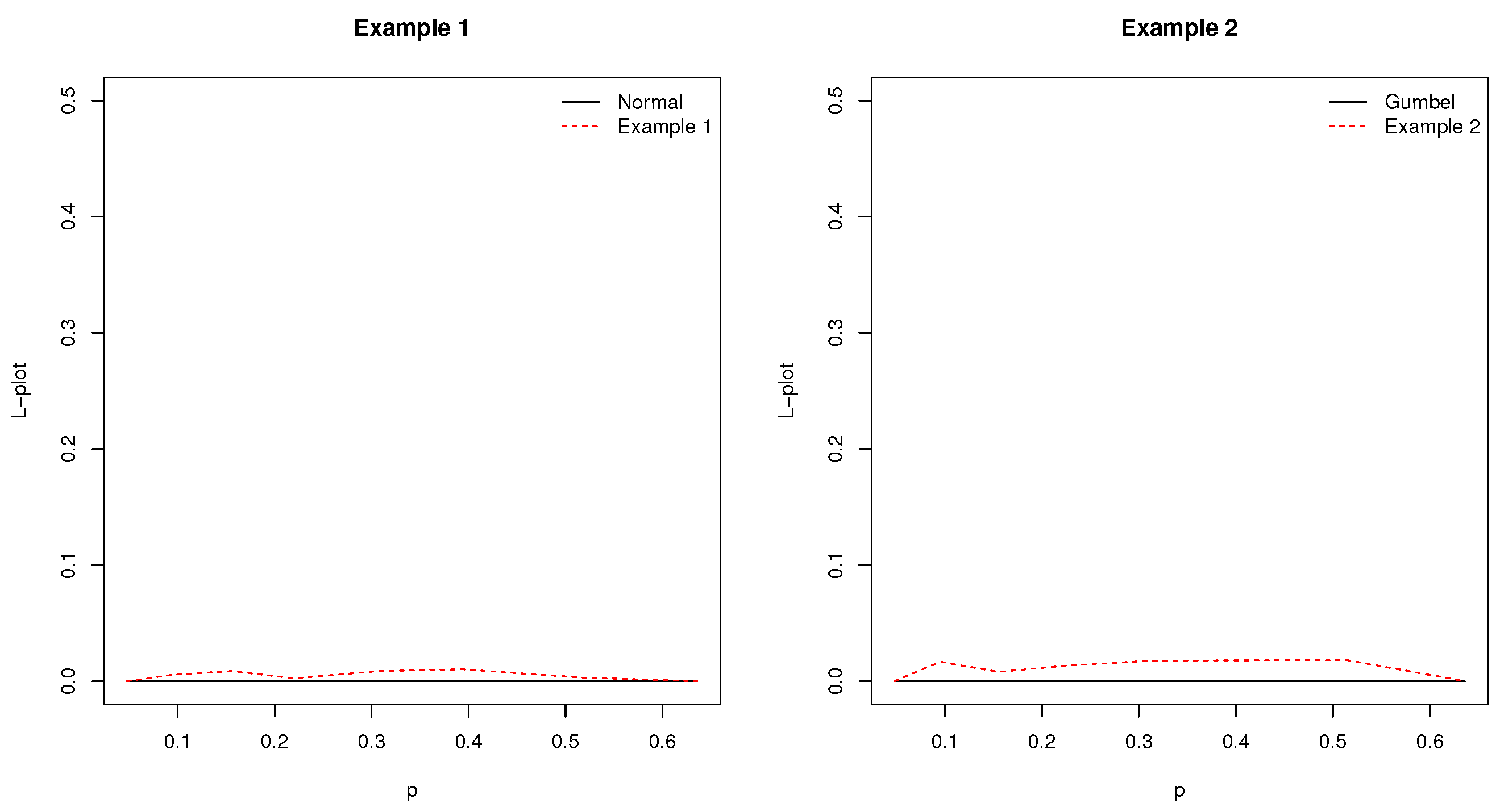
We can confirm this with $L-plot\left(p_{j:m:n}\right)$. The $L-plot\left(p_{j:m:n}\right)$ of Example 1 is presented in Figure 4. Figure 4 shows that the $L-plot\left(p_{j:m:n}\right)$ of Example 1 is closed to $L-plot\left(p_{j:m:n}\right)=0$. Thus, $L-plot\left(p_{j:m:n}\right)$ concludes that Example 1 follows NormDist.

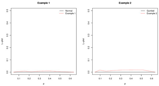
Figure 4. $L-plot\left(p_{j:m:n}\right)$ of examples.

Example 2 (log transformed insulating fluid test data)

The Example 2 data were previously studied by Refs. [11,23]. In Example 2, Refs. [11,23] generated a PrCsD of size $m=8$ from $n=19$. The PrCsD are given in Table 5.

Table 5. Example 2 data.

j	1	2	3	4	5	6	7	8
$R_j$	0	0	3	0	3	0	0	5
$x_{j:m:n}$	−1.66	−0.25	−0.04	0.27	1.02	1.58	1.99	2.87

The values of the TstSs and the corresponding p-values are presented in Table 6. Table 6 shows that all p-values are greater than significance level 0.05. Therefore, the given p-values support the $H_0$ of the GumDist for the data. This result is in agreement with the findings of Refs. [10,11,23].

Table 6. TstSs and the corresponding p-values for example 2.

	${\mathit{L}}_{\mathit{m}:\mathit{n}}^{+}$	${\mathit{L}}_{\mathit{m}:\mathit{n}}^{-}$	${\mathit{L}}_{\mathit{m}:\mathit{n}}^{\left(1\right)}$	${\mathit{L}}_{\mathit{m}:\mathit{n}}^{\left(2\right)}$	${\mathit{L}}_{\mathit{m}:\mathit{n}}^{\left(3\right)}$	${\mathit{L}}_{\mathit{m}:\mathit{n}}^{\left(4\right)}$	${\mathit{C}}_{\mathit{m}:\mathit{n}}^{+}$	${\mathit{C}}_{\mathit{m}:\mathit{n}}^{-}$	${\mathit{C}}_{\mathit{m}:\mathit{n}}$	${\mathit{K}}_{\mathit{m}:\mathit{n}}$	${\mathit{T}}_{\mathit{m}:\mathit{n}}^{\left(1\right)}$	${\mathit{T}}_{\mathit{m}:\mathit{n}}^{\left(2\right)}$
TstS	0.01254	0.02235	0.02235	0.03489	0.00013	0.00877	0.25443	0.02262	0.25443	0.27705	0.01197	0.07469
p-value	0.5780	0.4624	0.9195	0.8503	0.9269	0.9142	0.6789	0.8915	0.6789	0.8508	0.9512	0.9524

We are also able to confirm the $L-plot\left(p_{j:m:n}\right)$. The $L-plot\left(p_{j:m:n}\right)$ of Example 2 is presented in Figure 4. Figure 4 shows that the $L-plot\left(p_{j:m:n}\right)$ of Example 2 is closed to $L-plot\left(p_{j:m:n}\right)=0$. Thus, $L-plot\left(p_{j:m:n}\right)$ concludes that Example 2 follows GumDist.

6. Conclusions

The problem of examining how well the data fit a supposed distribution is very important, and it must be confirmed prior to any data analysis. Usually, we use a histogram or Q-Q plot for the assessment of data distribution. Furthermore, we use a GoF TstS. In life-testing or reliability studies, the observed failure time of test units may not be recorded in some situations. The GoF TstSs for completely observed data can no longer be used in PrCsD. In this paper, we suggest a GoF TstSs and a new plot method for the GoF test of LoScD based on PrCsD.

The proposed TstS is designed to be free of LoSc parameters, ensuring that distributions with these parameters remain unaffected by their specific values. Consequently, the standard distribution serves as the parameter value for the null distribution, ensuring that the power of the test remains consistent irrespective of the parameter value in the null distribution. The power of the suggested TstSs is estimated through MC simulations, and it is compared with that of the TstSs using the OrSts. As the parent distributions, we consider NormDist and GumDist. For testing the NormDist and GumDist, the alternative distribution is considered tDist with 4, 5, 6 and 7 DoF and LGamDist with ShPm 3, 6, 9 and ∞, respectively.

For testing the NormDist, the $L_{m:n}^{-}$ TstS possessed better power than Ref. [10]’s TstSs in a number of PrCs. $L_{m:n}^{-}$ TstS was found to be better than Ref. [10]’s TstSs in all PrCs. For testing the GumDist, the $L_{m:n}^{+}$ TstS possessed better power than Ref. [10]’s TstSs in a number of PrCs. $L_{m:n}^{+}$ TstS was found to be better than Ref. [10]’s TstSs in 64 out of 108 PrCs. Therefore, it can be seen that the TstSs using the LrCv are better than the TstSs using the OrSts. Moreover, the proposed method in this study not only provides test statistics but also incorporates graphical representations, allowing for the visual interpretation of results.

Although we have supposed that the LoScDs are GumDist and NormDist, any other LoScD can also be considered.

References

- Balakrishnan, N.; Aggarwala, R. Progressive Censoring: Theory, Methods and Applications; Birkhauser: Boston, MA, USA, 2000. [Google Scholar]
- Mahto, A.K.; Tripathi, Y.M.; Kizilaslan, F. Estimation of reliability in a multicomponent stress-strength model for a general class of inverted exponentiated distributions under progressive censoring. J. Stat. Theory Pract. 2020, 14, 1–35. [Google Scholar] [CrossRef]
- Algarni, A.; Elgarhy, M.; M Almarashi, A.; Fayomi, A.; R El-Saeed, A. Classical and bayesian estimation of the inverse Weibull distribution: Using progressive type-I censoring scheme. Adv. Civ. Eng. 2021, 2021, 1–15. [Google Scholar] [CrossRef]
- Almongy, H.M.; Alshenawy, F.Y.; Almetwally, E.M.; Abdo, D.A. Applying transformer insulation using Weibull extended distribution based on progressive censoring scheme. Axioms 2021, 10, 100. [Google Scholar] [CrossRef]
- Alam, I.; Ahmed, A. Inference on maintenance service policy under step-stress partially accelerated life tests using progressive censoring. J. Stat. Comput. Simul. 2022, 92, 813–829. [Google Scholar] [CrossRef]
- Moharib Alsarray, R.M.; Kazempoor, J.; Ahmadi Nadi, A. Monitoring the Weibull shape parameter under progressive censoring in presence of independent competing risks. J. Appl. Stat. 2023, 50, 945–962. [Google Scholar] [CrossRef] [PubMed]
- Dey, S.; Elshahhat, A.; Nassar, M. Analysis of progressive type-II censored gamma distribution. Comput. Stat. 2023, 38, 481–508. [Google Scholar] [CrossRef]
- Wang, B. Goodness-of-fit test for the exponential distribution based on progressively Type II censored sample. J. Stat. Comput. Simul. 2008, 78, 125–132. [Google Scholar] [CrossRef]
- Pakyari, R.; Balakrishnan, N. A general purpose approximate goodness-of-fit test for progressively type-II censored data. IEEE Trans. Reliab. 2012, 61, 238–244. [Google Scholar] [CrossRef]
- Pakyari, R.; Balakrishnan, N. Goodness-of-fit tests for progressively Type II censored data from location-scale distribution. J. Stat. Comput. Simul. 2013, 83, 167–178. [Google Scholar] [CrossRef]
- Lee, W.; Lee, K. Goodness-of-fit tests for progressively Type II censored data from a location-scale distributions. Commun. Stat. Appl. Methods 2019, 26, 191–203. [Google Scholar]
- Ma, Y.; Gui, W. Entropy-based and non-entropy-based goodness of fit test for the inverse rayleigh distribution with progressively type II censored data. Probab. Eng. Informational Sci. 2021, 35, 631–649. [Google Scholar] [CrossRef]
- Pakyari, R. Goodness-of-fit testing based on Gini Index of spacings for progressively Type-II censored data. Commun. Stat. Simul. Comput. 2023, 52, 3223–3232. [Google Scholar] [CrossRef]
- Qin, X.; Yu, J.; Gui, W. Goodness-of-fit test for exponentiality based on spacings for general progressive Type-II censored data. J. Appl. Stat. 2022, 49, 599–620. [Google Scholar] [CrossRef] [PubMed]
- Cho, Y.; Lee, K. Goodness-of-fit test for progressive censored data from an inverse Weibull distribution. J. Korean Data Inf. Sci. Soc. 2023, 34, 505–513. [Google Scholar]
- Fusek, M. Statistical power of goodness-of-fit tests for type I left-censored data. Austrian J. Stat. 2023, 52, 51–61. [Google Scholar] [CrossRef]
- Vaisakh, K.M.; Xavier, T.; Sreedevi, E.P. Goodness of fit test for Rayleigh distribution with censored observations. J. Korean Stat. Soc. 2023, 52, 794–815. [Google Scholar] [CrossRef]
- Atkinson, A.B. On the measurement of inequality. J. Econ. Theory 1970, 2, 244–263. [Google Scholar] [CrossRef]
- Gastwirth, J.L. A general definition of the Lorenz curve. Econometrica 1971, 39, 1037–1039. [Google Scholar] [CrossRef]
- Gail, M.H.; Gastwirth, J.L. A scale-free goodness-of-fit test for the exponential distribution based on the Lorenz curve. J. Am. Stat. Assoc. 1978, 73, 787–793. [Google Scholar] [CrossRef]
- Balakrishnan, N.; Ng, H.K.T.; Kannan, N. Goodness-of-fit tests based on spacings for progressively Type II censored data from a general location-scale distribution. IEEE Trans. Reliab. 2004, 53, 349–356. [Google Scholar] [CrossRef]
- King, J.R. Probability Charts for Decision Making; Industrial Press: New York, NY, USA, 1971. [Google Scholar]
- Nelson, W. Applied Life Data Analysis; John Wiley & Sons: New York, NY, USA, 1982. [Google Scholar]
Disclaimer/Publisher’s Note: The statements, opinions and data contained in all publications are solely those of the individual author(s) and contributor(s) and not of MDPI and/or the editor(s). MDPI and/or the editor(s) disclaim responsibility for any injury to people or property resulting from any ideas, methods, instructions or products referred to in the content. |
© 2024 by the author. Licensee MDPI, Basel, Switzerland. This article is an open access article distributed under the terms and conditions of the Creative Commons Attribution (CC BY) license (https://creativecommons.org/licenses/by/4.0/).