Enhancing Urban Intersection Efficiency: Visible Light Communication and Learning-Based Control for Traffic Signal Optimization and Vehicle Management

Abstract

This paper introduces a novel approach, Visible Light Communication (VLC), to optimize urban intersections by integrating VLC localization services with learning-based traffic signal control. The system enhances communication between connected vehicles and infrastructure using headlights, streetlights, and traffic signals to transmit information. Through Vehicle-to-Vehicle (V2V) and Infrastructure-to-Vehicle (I2V) interactions, joint data transmission and collection occur via mobile optical receivers. The goal is to reduce waiting times for pedestrians and vehicles, enhancing overall traffic safety by employing flexible and adaptive measures accommodating diverse traffic movements. VLC cooperative mechanisms, transmission range, relative pose concepts, and queue/request/response interactions help balance traffic flow and improve road network performance. Evaluation in the SUMO urban mobility simulator demonstrates advantages, reducing waiting and travel times for both vehicles and pedestrians. The system employs a reinforcement learning scheme for effective traffic signal scheduling, utilizing VLC-ready vehicles to communicate positions, destinations, and routes. Agents at intersections calculate optimal strategies, communicating to optimize overall traffic flow. The proposed decentralized and scalable approach, especially suitable for multi-intersection scenarios, showcases the feasibility of applying reinforcement learning in real-world traffic scenarios.

1. Introduction

Visible Light Communication (VLC) stands at the forefront of technological innovation, offering a novel approach to data communication by harnessing the intensity modulation of light emitted by Light Emitting Diodes (LEDs) [1,2]. This emerging technology holds tremendous potential across various applications due to its inherent simplicity in design, operational efficiency, and widespread geographical distribution. Particularly in the realm of vehicular communications, VLC finds a seamless integration as vehicles, streetlights, and traffic signals universally employ LEDs for both illumination and signaling purposes [3]. Here, communication and localization are performed using the streetlamps, the traffic signaling, and the head and tail lamps, enabling the dual use of exterior automotive and infrastructure lighting for both illumination and communication purposes [4,5].

Recent strides in traffic signal control have seen the successful application of reinforcement learning, yet most of these advancements have predominantly focused on optimizing vehicle traffic, neglecting the intricate dynamics of pedestrian flow within intersections [6]. Accurate estimation of pedestrian movement and positions remains a challenge, and existing traffic control algorithms often overlook the critical component of pedestrian traffic. This presents an opportunity for enhancing reinforcement learning-based traffic signal control systems to encompass both vehicular and pedestrian flows for more comprehensive intersection management.

The emergence of VLC localization presents a promising opportunity to revolutionize the efficiency, safety, and scalability of multi-intersection traffic signal control in environments with mixed traffic flows [7]. However, addressing coordination, scalability, and integration challenges remains paramount. In response, we introduce a pioneering solution: the Vehicular-VLC (V-VLC) distributed reinforcement learning-based traffic signal control system with pedestrian access. This innovative approach tackles these challenges he ad-on by seamlessly integrating advanced VLC localization technology with cutting-edge reinforcement learning algorithms.

The goal is to contribute to the advancement of Intelligent Transport Systems (ITS) technology, striving to optimize traffic safety and efficiency through enhanced situation awareness and reduced accidents via vehicle-to-vehicle (V2V), vehicle/pedestrian-to-infrastructure (V/P2I), or infrastructure-to-vehicle/pedestrian (I2V/P) communications [8,9,10]. Recognizing the inefficiencies inherent in traditional traffic light cycle controls, such as long delays and energy wastage, the focus shifts to dynamic adjustments based on real-time traffic information. The ultimate goal is to elevate safety and throughput at intersections through cooperative driving strategies [11,12]. What sets our approach apart is its comprehensive consideration of diverse traffic participants, including pedestrians. Traditional traffic signal control systems often overlook pedestrian mobility, leading to inefficiencies and safety concerns. Our model incorporates a novel pedestrian mobility model tailored for outdoor scenarios, analyzing various pedestrian behaviors and seamlessly integrating them into the established traffic signal control scheme designed for vehicular traffic. Moreover, the routing algorithm embedded within our model adopts a user-centric approach, guiding pedestrians to their destinations while prioritizing routes that are more appealing from a pedestrian perspective. This not only enhances pedestrian satisfaction but also optimizes overall traffic flow and safety. Our model’s versatility is a key strength. It is inherently adaptable to any outdoor pedestrian scenario, provided sufficient street database and pedestrian traffic information are available. Through rigorous validation, including a comprehensive case study in Lisbon’s downtown area [13], we have demonstrated the efficacy and scalability of our mobility model in real-world settings.

In summary, our Vehicular-VLC (V-VLC) distributed reinforcement learning-based traffic signal control system represents a significant advancement in traffic management technology. By bridging the gap between VLC localization, reinforcement learning, and pedestrian mobility modeling, we not only address current challenges but also pave the way for safer, more efficient, and more inclusive transportation systems.

The paper is organized as follows. After the introduction, in Section 2, the main V-VLC challenges are presented, and in Section 3, we delve into the intricacies of the V-VLC system, detailing its architecture, communication protocol, and coding/decoding techniques. Experimental results, system evaluations, and a Proof of Concept (PoC) in the form of a phasing traffic flow diagram based on V-VLC are presented in Section 4. Section 5 explores an agent-based dynamic traffic control simulation using an urban mobility simulator tool. Finally, Section 6 encapsulates the paper’s findings and conclusions, emphasizing the potential of V-VLC in revolutionizing traffic signal control and intersection management.

2. Traffic Control Challenges: Addressing Pedestrian Dynamics and Muti-Intersection Scenarios

The optimization of traffic control algorithms, particularly those leveraging reinforcement learning, has predominantly centered around vehicular traffic flow, often neglecting the intricate dynamics of pedestrian movement within intersection spaces. This oversight presents a critical challenge that necessitates the development of reinforcement learning-motivated traffic signal control systems with explicit consideration for pedestrian access.

The key challenges to solving this problem are:

(1)

What is special about pedestrian traffic as opposed to vehicle traffic?

(2)

How can we exploit these specialties to optimize the efficiency, safety, and scalability of traffic signal control in the multi-intersection scenario?

2.1. Pedestrian Traffic Dynamics and Multi-Intersection Complexity

One major obstacle arises from the unique nature of sidewalks. Unlike traffic lanes, which are typically one-way, sidewalks accommodate two-way pedestrian movement, adding complexity to determining the direction of pedestrian flow. The challenge is further compounded by the inherent difficulty in discerning pedestrian movement direction accurately. Despite localization technologies offering ample range and high-accuracy movement recognition, uncertainties persist, and balancing safety and efficiency in the interplay between pedestrian and vehicular traffic remains an open question.

The disparities between pedestrians and vehicles, including differences in speed, physical volume, and movement patterns, introduce additional challenges. Pedestrians and vehicles may impede each other, leading to reduced traffic flow efficiency and potential safety hazards. Striking an optimal balance between these two traffic components poses a significant challenge that demands careful consideration [14].

Another challenge arises in the context of multi-intersection scenarios. While a straightforward approach involves a single agent controlling traffic lights across all intersections, this approach is hindered by scalability issues. The exponential growth of state and action spaces becomes impractical in real-time control applications. While single-intersection optimization schemes demonstrate scalability within their domain, extending their effectiveness to multi-intersection environments requires innovative solutions.

Researchers have explored collaborative mechanisms to address this challenge, incorporating factors such as queue length in neighboring intersections and modeling relationships between these intersections. These efforts aim to achieve a balance between scalability and efficiency in multi-intersection scenarios, acknowledging the need for a more nuanced approach to optimize traffic control. Our adaptive traffic control strategy aims to respond to real-time traffic demand through current and predicted future traffic flow data modeling. Compared with the traffic flow and occupancy information provided by the fixed coil detector in the traditional traffic environment, the adaptive traffic control system in the V2X environment can collect more detailed data such as vehicle position, speed, queuing length, and stopping time. While V2V links are particularly important for safety functionalities such as pre-crash sensing and forward collision warning, I2V/P links provide the CV and the pedestrians with a variety of useful information [15,16].

2.2. Innovative Solutions: V-VLC Integration

With the advancement of wireless communication technologies and the development of the V2V and V2I systems, called Connected Vehicles (CV) [17], there is an opportunity to optimize the operation of urban traffic networks through cooperation between traffic signal control and driving behaviors. In response to these challenges, this paper introduces a novel approach that combines Visible Light Communication (VLC) localization services with learning-based traffic signal control. The objective is to achieve comprehensive control over both pedestrian and vehicular traffic, with a focus on reducing waiting times and enhancing overall traffic safety in multi-intersection scenarios.

To develop an intelligent control system model that facilitates safe vehicle management through intersections using V2V, V/P2I, and I2V/P communications, Reinforcement Learning (RL) concepts are utilized. RL is a training method that involves rewarding desired behaviors and/or punishing undesired ones [18,19]. To assess the effectiveness of the proposed V-VLC system in multi-intersection scenarios, we utilize a simulator Simulation of Urban MObility (SUMO) [20] where the simulations are agent-based. As the agent gains experience, it learns to avoid negative situations and focus on positive ones. The traffic lights in SUMO are controlled by the learning agent based on its decisions, and the overall flow of traffic is described while rewarding the actions of the traffic lights control agent. The agent’s goal is to explore new states while maximizing its total reward to develop the best possible policy. A dynamic phasing diagram and a matrix of states based on the total accumulated time are presented to illustrate the concept.

Comparative analyses against traditional methods showcase advantages in multiple dimensions, including waiting time, travel time for both vehicle and pedestrian traffic flows, and overall safety scores. Additionally, the paper validates design choices through comparisons with several variants of the proposed method, providing insights into the robustness and adaptability of the approach.

3. Traffic Controlled Intersection

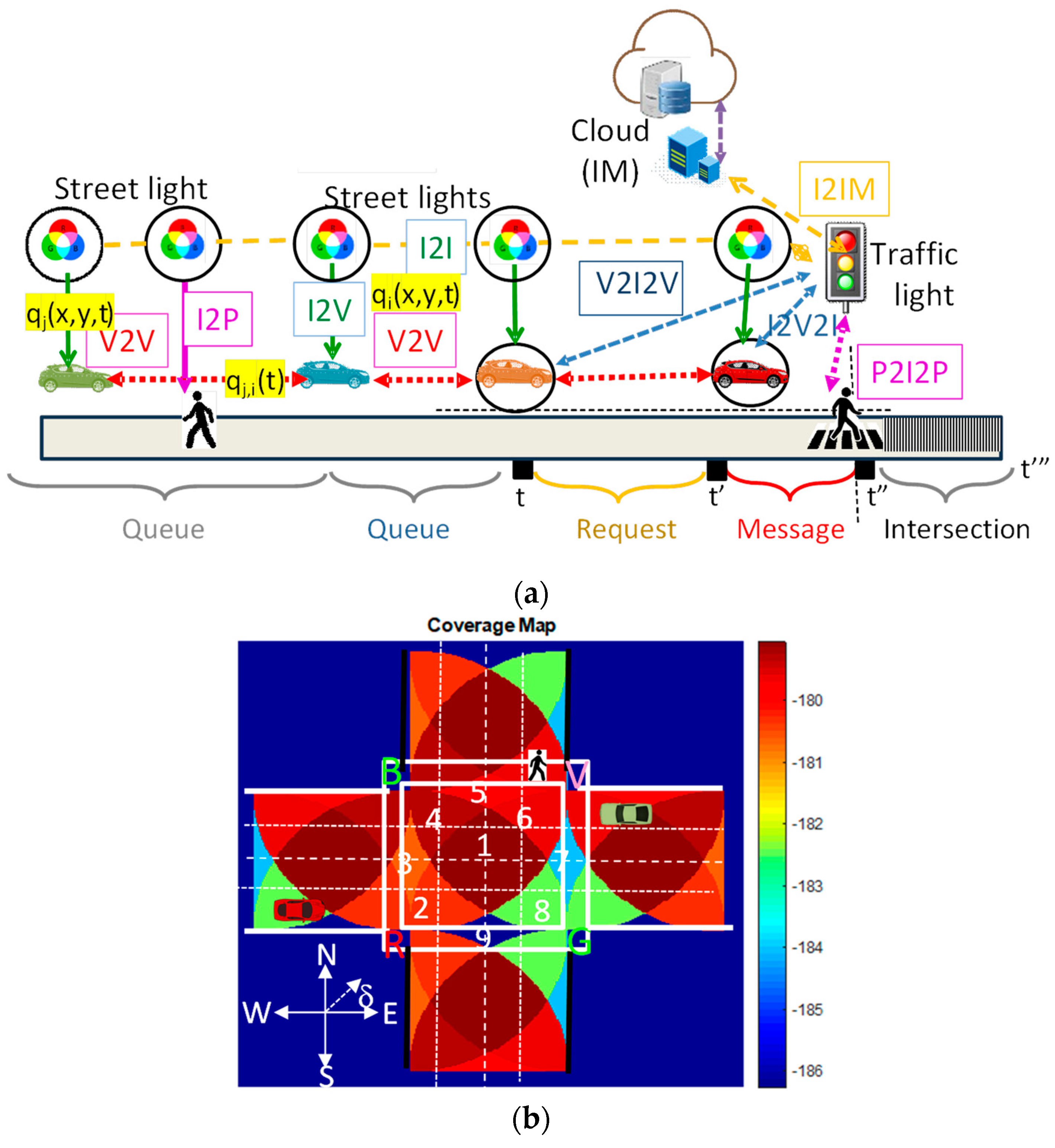
3.1. V-VLC Communication Link

The device-to-cloud communication system depicted in Figure 1a embodies an architecture designed to facilitate seamless data exchange and processing between various components of the traffic control infrastructure. Central to this architecture is a mesh cellular hybrid structure, which encompasses two distinct types of controllers strategically deployed at streetlights to optimize system performance and scalability.

The system employs two types of controllers [21]:

• Mesh Controllers: Positioned at the streetlights, at strategic intervals along roadways, the “mesh” controller serves as a pivotal node in the network, responsible for relaying messages to vehicles traversing its vicinity. The mesh controller efficiently forwards data packets to nearby vehicles, ensuring timely dissemination of critical information such as geo-distribution and real-time load balancing (q(x,y,t)) and traffic messages.
• Mesh/Cellular Hybrid Controllers: At the traffic lights, operating at the intersection of mesh and cellular networks, the “mesh/cellular” hybrid controller assumes a multifaceted role within the system architecture. Primarily functioning as a border-router for edge computing (V2I), this controller not only facilitates seamless integration between mesh and cellular networks but also serves as a gateway for data exchange between edge devices and the central cloud infrastructure (I2IM). By leveraging the hybrid nature of its connectivity, the mesh/cellular controller enables robust and resilient communication pathways, ensuring uninterrupted data flow across the network.

In conjunction with the network architecture, the proposed system harnesses embedded computing platforms to enhance data processing capabilities and enable advanced functionalities at the edge of the network. Additionally, the design encourages peer-to-peer communication (I2I) among vehicles, enhancing data sharing and collaboration within the network. These embedded platforms play a pivotal role in executing a myriad of tasks, including processing sensor data and algorithmic computations in real-time, interfacing with sensors deployed across the traffic infrastructure, enabling precise detection of traffic flow patterns and pedestrian movements, and enabling the geo-distribution and real-time load balancing. By processing data at the edge, the system reduces response times and eases the load on the central cloud infrastructure.

A Vehicular VLC system (V-VLC) comprises a transmitter that generates modulated light and a receiver located in infrastructures, driving cars, and pedestrians to detect the received light variation. Both the transmitter and receiver are connected through the wireless channel. In this system, the light produced by the LED is modulated using ON-OFF-keying (OOK) amplitude modulation [22]. The environment is defined by a cluster of square unit cells arranged in an orthogonal geometry. Different data channels are provided by tetra-chromatic white light (WLEDs) sources positioned at the corners of the square unit cells [23,24] distributed along the road and at the crossroads. Tetra-chromatic white light (WLEDs) sources, framed at the corners of a square unit cell, provide different data channels. They consist of red, green, blue and violet chips and combine the lights in correct proportion to generate white light. At each node, only one chip of the LED is modulated for data transmission: the Red (R: 626 nm), the Green (G: 530 nm), the Blue (B: 470 nm), or the Violet (V: 390 nm). Modulation and digital-to-analog conversion of the information bits is conducted using signal processing techniques. Transmitters and receivers’ 2D relative positions are displayed in Figure 1a. The coverage map in a four-legged intersection is displayed in Figure 1b. The coded nine possible overlaps (#1–#9), defined as fingerprint regions, as well as the possible receiver directions (Cardinal points; δ), are also pointed out for the intersection [25]. The input of the V-VLC system consists of coded signals sent by transmitters such as streetlights and traffic lights. These signals are intended to communicate directly with identified vehicles (I2V) and pedestrians (I2P) or indirectly between vehicles through the headlights (V2V). Each transmitter sends an I2V message that includes the synchronism, its physical ID, and the traffic information. When a probe vehicle/pedestrian enters the streetlight’s capture range, the receiver replies to the light signal and assigns a unique ID and a traffic message. To manage the passage of vehicles crossing the intersection, queue/request/response mechanisms and temporal/space relative pose concepts are employed. The coded signals are received and decoded by PIN-PIN photodetectors with light-filtering properties [5] embedded into the mobile receivers. The MUX receiver multiplexes the different optical channels, performs different filtering processes (amplification, switching, and multiple signals, finds the centroid of the received coordinates, and stores it as reference point positions. Nine reference points for each unit cell are identified, giving a fine-grained resolution in the localization of the mobile devices across each cell (see Figure 1b). So, the input is the coded signal sent by the transmitters to an identified vehicle/pedestrian (I2V/P) and allows the identity of the position in the network q(x_i,y_j,t) inside the unit cell (#1–#9) and the direction, (cardinal points) that guides the driver/pedestrians orientation across his path.

3.2. Scenario and Environment for the Simulation

The simulated scenario is multi-intersections, as displayed in Figure 2, based on two 4-way intersections, each with two lanes on each arm, approaching the intersection from compass directions, leaving two lanes on each arm. Each arm is 100 m long. On every arm, each lane defines the possible directions that a vehicle can follow: the right lane enables vehicles to turn right or go straight, while on the left lane, the left turn is the only direction allowed. In the center of the intersection, a traffic light system controlled by the IM (also known as the agent) manages the approaching traffic. Emitters (streetlamps) are located along the roadside.

Pedestrian lanes, waiting corners, and crosswalks were also considered. Diagonal crossings, also called pedestrian scrambles, were used. This is a type of crossing in which a dedicated phase allows pedestrians to cross the intersection in every direction at the same time [26]. During this phase, all vehicular traffic is stopped. This type of signalized crossing avoids conflicts between pedestrians and turning vehicles. It is applied only at intersections with high pedestrian volume and should be designed to provide enough space for large numbers of people to gather on the sidewalk corners.

Based on clusters of square unit cells, an orthogonal topology was considered to define the environment. Each transmitter (X_i,j) carries its own color, X (Red, Green, Blue, Violet), as well as its horizontal and vertical ID position in the surrounding network (i,j). A matrix of i lines and j columns was used to define the orthogonal topology used for the environment during the Proof of Concept (PoC). It was assumed that the crossroads are located at the intersections of line 4 with column 3 and column 11, respectively.

In Figure 2, the two four-legged double intersections and the environment with the optical infrastructure (X_ij), the generated footprints (1–9), the connected vehicles (CV), and the connected pedestrians (CP) are drafted. We considered four distinct traffic flows along the cardinal points. Road request and response segments offer a binary (turn left straight or turn right) choice. According to the simulated scenario, each car represents a percentage of traffic flow. Based on our assumptions, there is a total influx of 2300 cars per hour approaching the intersections, with 80% originating from the east and west directions. Subsequently, 25% of these cars are expected to make either a left or right turn at the intersection, while the remaining 75% will continue straight. The pedestrian influx is about 11,200 per hour generated in both vertical roads and across the intersection in all directions. The average speed is 3 Km/h.

To illustrate the various traffic flows, let’s consider the following scenario in a cycle: from the twenty-four vehicles approaching from the West (W), twenty vehicles (a_i) follow a straight path (represented by the red flow), and four vehicles (c_i) make a left turn only (depicted by the yellow flow). In the green flow, vehicles from the East (E) are represented by the b_i category. Thirteen of these vehicles move straight, while two execute a left turn. In the orange flow, originating from the South (S), there are six vehicles (e_i). Among these, two vehicles take a left-turn approach, and the remaining four continue straight. Lastly, in the blue flow, thirteen vehicles (f_i) arriving from the North are considered. Nine of these vehicles continue straight, while four execute a left turn at the intersection. This breakdown exemplifies the distribution of traffic in each flow, depicting the movements of vehicles in terms of straight paths and left turns at the intersection. It is assumed that a₁, b₁, and a₂ make up the top three requests, followed by b₂, a₃, and c₁ in fourth, fifth, and sixth place, respectively. In seventh, eighth, and ninth request places are b₃, e₁, and a₄, respectively, followed in tenth place by c₂. The penultimate request is a₅, and the last one is f₁.

3.3. Multi-Cooperative Localization

In the described system (depicted in Figure 1 and Figure 2), streetlights, functioning as geo-transmitters, are strategically positioned along the roadside, 20 m apart. Each LED transmitter emits an I2V message, encompassing synchronization, physical ID, and traffic information. When a probe vehicle or pedestrian enters the capture range of a streetlight, the receiver promptly responds by assigning a unique ID (q_i(x,y,t)) and providing relevant traffic information.

As the vehicle or pedestrian approaches an intersection, they initiate a request for permission to cross (V/P2I). In response, an acknowledgment (response, I2V/P) is dispatched from the traffic signal to the head vehicle’s in-car application or to the pedestrians. Following this, the vehicle must adhere to specified occupancy trajectories, denoted as footprint regions (refer to Figure 2).

If a crossing request poses a potential collision risk with approved vehicles, the control manager exercises caution by delaying the response until the risk is adequately mitigated. Vehicle speed is calculated by measuring the actual traveled distance over time, utilizing the IDs of transmitters for tracking, denoted as q_i(x,y,t). In scenarios involving multiple neighboring vehicles, the mesh node employs indirect V2V relative pose estimations, represented as q_ij(t), leveraging data from each neighboring vehicle [27]. The notations q(t), q(t′), q(t″), q(t‴) denote the vehicle pose estimation (location and orientation) at times t, t′, t″, and t‴ (request, response, enter, and exit times), respectively. All requests include vehicle positions, directions, and approach speeds. In cases where followers exist, the request message from the leader includes the poses and speed previously received by V2V. This information serves as an alert to the controller for a subsequent request message (V2I) confirmed by the following vehicle. To determine delays, the number of vehicles queuing in each cell at the beginning and end of the green time is ascertained through V2V2I observation, as illustrated in Figure 1a.

The introduction of VLC between pedestrians, vehicles, and the surrounding infrastructure allows the direct monitoring of critical points that are related to queue formation and dissipation, relative speed thresholds, inter-vehicle spacing, and pedestrian corner density, increasing road safety. Critical points where traffic conditions may change include instances where a pedestrian stops and joins the waiting corners. Through P2I2P communication, the travel time influencing different sidewalks can be calculated, and real-time data about speed and waiting times are analyzed using the ID’s transmitter tracking. Receivers compute geographical positions in successive instants (path) and infer the pedestrian’s speed.

3.4. Communication Protocol

To encode the information, an On-Off Keying (OOK) modulation scheme was employed, utilizing synchronous transmission with a 64-bit data frame. To transmit the signals, each infrastructure is equipped with tetrachromatic LEDs (Figure 1b), enabling the simultaneous transmission of four signals. This configuration requires a receiver capable of actively filtering each channel, providing a four-fold increase in bandwidth.

Each of the RGBV signals sent has a wavelength-calibrated amplitude that defines it. Since each VLC infrastructure has four independent emitters, the optical signal generated in the receiver can have one, two, three, or even four optical excitations, resulting in 2⁴ different optical combinations and 16 different photocurrent levels at the photodetector [24]. Filtering is accomplished using a PIN-PIN demultiplexer. The PIN-PIN demultiplexer plays a crucial role in the decoding process, ensuring accurate retrieval of the original message. It receives the combined OOK signals and is armed with prior knowledge of the calibrated amplitudes and decodes the sent message.

The communication protocol defines the structure and rules governing the exchange of information. It likely includes specifications for the synchronization, identification, and payload portions of the transmitted frame. The communication protocol is presented in

Table 1. Communication protocol.

		COM	Position
L2V	Sync	1	x	y	END	Hour	Min	Sec	Payload	(32 bits)					EOF
V2V	Sync	2	x	y	Lane (0–7)	Nº Veic.	END	Hour	Min	Sec	Car IDx	Car IDy	nº behind		EOF
V2I	Sync	3	x	y	TL (0–15)	Nº Veic.	END	Hour	Min	Sec	Car IDx	Car IDy	nº behind		EOF
I2V	Sync	4	x	y	TL (0–15)	ID veic	END	Hour	Min	Sec	Car IDx	Car IDy	nº behind	Phase	EOF
P2I	Sync	5	x	y	TL (0–15)	Direct.	END	Hour	Min	Sec	payload				EOF
I2P	Sync	6	x	y	TL (0–15)	Phase	END	Hour	Min	Sec	Payload				EOF

.

Each frame depends on the kind of communication (1–6) and starts with a synchronization block, followed by various identification blocks, and ends with an EoF block. The traffic message contains critical information related to vehicles and pedestrians’ movements. The entire structure ensures a systematic and standardized communication protocol for the VLC system.

1-Frame Structure:

• Start of Frame (SoF): The frame begins with a synchronization block of 5 bits, indicated by the pattern [10101]. This is used to synchronize the receivers and identify the start of a new frame.
• Identification (ID) Blocks: These blocks encode information using binary representation for coded decimal numbers. Information includes the type of communication, localization of transmitters (x, y coordinates), and timeline information (END, Hour, Min, Sec). The time sub-block begins with the pattern [111] to alert the decoder that the following bit sequence (6 + 6 + 6) corresponds to time identification rather than payload.
• Other ID Blocks: These include the necessary number and temporary identification of vehicles following the leader: Information related to the occupied lane (Lane 0–7), traffic signal requested (TL 0–15), cardinal direction, or active phase provided by the infrastructure in a “response” or “request” message at the intersection.
• 2-Traffic Message (Body of the Message): This block includes additional information:
• Vehicle Information: x, y coordinates and order of cars behind the leader that request/receive permission to cross the intersection (CarIDx, CarIDy, n° behind).
• Traffic information (payload); Road Conditions; Average Waiting Time; Weather Conditions:
• End of Frame (EoF): The frame concludes with a 4-bit EoF block, defined by the pattern [0000], indicating the end of the frame.

3.5. Transmitted and Decoded VLC Signals

In Figure 3a, the intersection drafts with the possible vehicles (color arrows) and pedestrians (dotted lines) trajectories, coded lanes (L 0–7), and traffic signals (TL 015) are displayed. In Figure 3b, a visual representation unfolds, elucidating the sequential progression of phases within the intersections. This orchestrated flow adheres to a structured cycle length comprising an exclusive pedestrian phase and eight distinct vehicular phases divided into two blocks whose order depends on the dynamic traffic flow. Each of these phases is further intricately subdivided into discrete time sequences or states, delineating a comprehensive temporal framework for the intersection’s operation [28].

Based on the measured photocurrent signal from the photodetector, decoding the received information is necessary. To achieve this, a calibration curve is established beforehand. Figure 4a illustrates the calibration curve, which incorporates 16 distinct photocurrent thresholds resulting from the combination of the four modulated RGBV signals emitted by the VLC emitter [24]. The correspondence between each threshold and the photocurrent level is highlighted on the right side of Figure 4a.

The received MUX signal, along with the coded optical signals transmitted, is displayed. The message within the frame begins with a header labeled “Sync,” consisting of a 5-bit block [10101] imposed simultaneously on all emitters. In the calibration block (the second block), four calibrated R, G, B, and V optical signals are transmitted concurrently. The bit sequence is chosen to encompass all sixteen possible combinations of the four RGBV input channels (2⁴). In the final block, a random message is transmitted.

Periodic retransmission of the calibration curve is necessary to ensure correspondence with the output signal and precise decoding of the transmitted information. By comparing the calibrated levels (d₀–d₁₅) with the assigned 4-digit binary [RGBV] codes (indicated on the right side of Figure 4a), decoding becomes straightforward, and the message can be deciphered [24].

Taking into account Figure 2 and Figure 3 and to illustrate the communication protocol (Table 1) and the technique for decoding calibrated signals emitted by transmitters, Figure 4b displays the decoded optical signals (at the top of the figures) and the signals received (MUX) by the receivers in a V2V (code 2) and V2I (code 3) communication scenario involving a leader vehicle a_o at position (R_3,10,G_3,11,B_4,10). This vehicle is communicating with the agent at the second intersection on lane L0 (direction E) at 10:25:46 and is followed by three other vehicles, V₁, V₂, and V₃, with the same direction, located at positions, R_3,8, G_3,6, and R_3,4, respectively.

In Figure 4c, the responses (I2V and I2P) from two traffic lights (TL10 and TL13) to the crossing request from the preceding vehicle a_o (R_3,10,G_3,11,B_4,10) and a pedestrian q₁ located in the “waiting corner” of the first intersection (R_3,4,G_3,5) are exemplified. These responses were sent at 10:25:46 and 10:28:66, respectively.

4. Dynamic Traffic Flow Control Simulation

This section aims to showcase a dynamic control system model designed to enhance the secure management of both vehicular and pedestrian traffic at intersections. The dynamic system effectively simulates the anticipated outcomes resulting from the application of VLC (Visible Light Communication) technology to both vehicles and pedestrians. Utilizing information gathered from V2V (Vehicle-to-Vehicle), V2I (Vehicle-to-Infrastructure), and I2V (Infrastructure-to-Vehicle) communications, the Intersection Manager (IM) strategically makes decisions regarding the activation of specific phases. This decision-making process prioritizes lanes with higher traffic, adhering to a predetermined sequence of phases illustrated in Figure 3b. Furthermore, an in-depth study has been conducted to analyze the system’s performance during both high and low-traffic cycles, with the objective of estimating the number of vehicles that could be efficiently managed within a one-hour timeframe.

4.1. SUMO Simulation: State Representation and Cycle and Phases Durations

The SUMO simulation environment, depicted in Figure 2, is adapted from a real-world setting in Lisbon [13,29,30]. This simulation scenario accounts for the impact of roads on traffic flow at two intersections. Specifically, the roads, referred to as the target road (W-E arm), dynamically influence traffic flow. The historical traffic state from other roads affecting the target road is limited in time, with the E-W being considered as the target road in this context. The transmission of traffic flow and traffic waves measures the duration for which the traffic state of other roads influences the target road within the same period. As traffic continuously enters the system, the composition of traffic flow on the target road undergoes changes over time and impacts the cycle length in both intersections. To enhance traffic flow conditions, a modification was introduced to the initially proposed phases (refer to Figure 3). This modification entails an immediate transition from the pedestrian phase (Ph0) to the N > S phase (Ph4), followed by the remaining phases in both intersections. Through adjustments to the phase sequence and optimization of the traffic light control strategy based on simulation results, enhancements in traffic flow, congestion reduction, and overall intersection performance can be achieved.

In terms of vehicle circulation, all vehicles are assumed to have an average speed of 10 m/s. However, when vehicles approach the traffic light at the start of the cycle, specifically during pedestrian evacuation, their speed is reduced to 5 m/s. Considering this adjusted speed, it is estimated that each vehicle requires approximately three seconds of green light to pass through the traffic signal. By incorporating this information into the incentive system, the agent is encouraged to make decisions that optimize traffic flow, minimize delays, and ensure efficient use of green light time, thereby enhancing overall intersection efficiency.

To introduce pedestrians into the dynamic system, two scenarios previously tested for vehicles were considered: the High and Low scenarios. The High scenario, with a cycle duration of 120 s, dispatches 76 cars, equivalent to 2300 cars per hour. The second scenario, lasting 88 s, dispatches 44 cars, equivalent to 1800 cars per hour. For each intersection, a pedestrian flow of 7200 at C1 and 4000 at C2 was generated [29]. Pedestrians were introduced only on the N and S roads (in both directions) at various distances from the intersection, simulating a scenario more reflective of reality where pedestrians start from different points. All pedestrians are introduced into the SUMO simulator with a speed of approximately 1 m/s, equivalent to 3 km/h, a value close to reality.

The state of the agent describes a representation of the situation of the environment in a given agentstep t, and it is usually denoted with s_t. To allow the agent to effectively learn to optimize the traffic, the state should provide sufficient information about the distribution of cars on each road. Figure 5 illustrates the complete state representation for the target road of the intersections during a simulated timeframe. The representation involves discrete cells for “response”, “request”, and “queue” zones, enabling the detection of vehicle entry into oncoming lanes. Before reaching the intersection’s stop line, each lane is divided into 5 cells (0/message, 1/request, 2–5/queues). A dedicated traffic light is associated with each lane, resulting in a total of 40 state cells during simulation, with lanes labeled as L/0–7 and traffic lights as TL/0–15.

During the simulation, an array is used to store the state of all vehicles at a given time, with states assigned to each vehicle. The state of a vehicle denoted as “v_i”, where “i” represents the order of the crossing request, is represented by a two-digit string. The first digit indicates the lane the vehicle is in, while the second digit represents its position within the lane. Taking into account Figure 4, the states of leader a₀ (in lane L0) and the following would be represented as v₁₅ = “00”, v₁₆ = “02”, v₁₇ = “03” and v₁₈ = “04”, respectively, to which corresponds Phase 2.2 (Figure 3b). So, the IM receives requests (V2I: exemplified in Figure 4a) for access to the intersection from all the leading vehicles and pedestrians at different times (t_x1 in Figure 1a). This V2I information provides the agent (IM) with precise location and speed data of all the leader vehicles, as well as the location and speed data of their followers, which is communicated through V2V communication (Figure 5a). This data enables the IM to anticipate the initial arrival times and speeds of vehicles at different sections of the intersection.

The Intersection Manager (IM), functioning as the agent, orchestrates traffic signals to ensure efficient and safe movement within the intersection. For effective traffic optimization learning, the state representation encompasses information about the environment, vehicle distribution derived from V-VLC received messages (refer to Table 1 and Figure 4b), and the proposed phasing diagram guiding agent actions (Figure 3b). The primary objective is to minimize the accumulated total waiting time in each intersection arm, calculated based on vehicle speed and queue alerts. The reward function considers the difference in accumulated waiting time between the current and previous steps in all the lanes, with negative rewards indicating higher waiting times. The agent learns to optimize traffic by taking actions (dynamic phases) based on the current state, with training involving stored data samples to improve decision-making. The decisions are communicated to the drivers and pedestrians through VLC response messages (Figure 4b), where the vehicle ID is assigned.

The SUMO application programming interface (API) allows interfacing with external programs, facilitating interaction with the simulation environment. SUMO supplies diverse statistics pertaining to overall traffic flow, and it offers various outputs, including diagrams that depict the duration of each state or color of traffic lights throughout the simulation. Utilizing the simulation scenario presented in Figure 2 and Figure 5, a state diagram was generated for the scenario with the highest traffic, encompassing both vehicles and pedestrians, using the SUMO simulation.

The traffic light diagram (Figure 6) typically illustrates the arrangement of the traffic lights (red, green, or yellow) along a cycle at an intersection and their corresponding signal phases (red, yellow, green). They serve as a visual aid for understanding how traffic signals control the flow of vehicles through an intersection, helping to optimize signal timing, reduce congestion, and improve overall traffic safety. Along a cycle, the traffic lights are depicted horizontally as colored lines or boxes. The colors of the traffic lights indicate the current signal phase for each traffic light (TL:0–15, at the left hand), with red, yellow, and green lights representing stop (red lines), prepare to stop (yellow boxes), and go (green boxes), respectively. To illustrate the sequence of signal phases, lines are drawn between the traffic lights, indicating the progression of the signal cycle. They show that when one set of lights turns green, another set turns red to facilitate the safe movement of traffic through the intersection. Figure 6a,c display the phase diagrams for the two connected intersections, C1 and C2, during two cycles of 120 s. Figure 6b provides an overview of the SUMO environment during a simulation with high pedestrian and medium vehicle traffic flows. As can be observed in the diagrams, it is possible to distinguish the different cycles that occur during the simulation. It always begins with a pedestrian phase, during which some individuals have the opportunity to cross the crosswalk, turning red for pedestrians starting from 11 s. Then, phases dedicated to vehicles take place until it concludes at 123 s. At this moment, the second cycle begins, with the pedestrian phase becoming active again. The same process repeats until 247 s, marking the end of this second cycle and the initiation of a third cycle. These diagrams align with the analysis conducted for pedestrians that follows.

4.2. SUMO Simulation: VLC Pedestrian Incorporation

To investigate the behavior of pedestrians in the environment, two variables were considered: average speed of pedestrians and halting. The first allows observing the influence of the cycle durations of each vehicle scenario on pedestrian speed, and the second enables the analysis of the number of people who are stationary in waiting zones across all intersections over time, giving insight into the number of people per square meter in each of the waiting zones.

Figure 7a illustrates the MUX signal sent to the traffic lights (TL’s) by pedestrians to cross both intersections (C1 and C2) while waiting in the corners (P_1,22I). In this figure, the top part displays the decoded messages, and on the right-hand side, the content of the message is outlined. Furthermore, Figure 7b demonstrates the MUX signal received by the traffic lights (I2P_1,2). The top part of the figure showcases the decoded messages, while the right-hand side provides a draft of the message content. This visual representation helps to understand the communication between pedestrians waiting in the corners and the corresponding traffic lights, providing insights into the signals exchanged for pedestrian crossings at both intersections (C1 and C2).

This representation provides insight into the communication dynamics between pedestrians and traffic lights at different intersections. The results reveal that the pedestrian begins walking on the sidewalk lane towards the west (W) with the intention of crossing through TL14, waiting in the designated area at positions R_3,12-G_3,13. At precisely 10:25:44, the pedestrian initiates communication with the traffic light (P₂2I), and within a second, by 10:25:45, a response is received (I2P₂). The pedestrian patiently remains in the waiting zone until the pedestrian phase becomes active.

Upon receiving information from the traffic light, it becomes evident that the current active phase is N-S (Phase 1), signifying that the pedestrian did not arrive in time for their designated phase (Phase 0). Consequently, the pedestrian is required to wait for an estimated 120 s before being granted the opportunity to cross. Subsequently, the pedestrian crosses the crosswalk, covering the distance to the next intersection in approximately 1 min and 50 s. Upon arrival, the pedestrian waits in the designated waiting zone at position R_3,4-G_3,5 until the pedestrian phase becomes active once again. At 10:28:35, the pedestrian establishes communication with traffic light TL13 at the C1 (P₁2I). The traffic light promptly responds (I2P₁) at 10:28:36, providing crucial information that the currently active phase is the final one in the cycle (Phase 6). These interactions highlight the effectiveness of the pedestrian’s communication with the traffic lights, enabling them to stay informed about the active phase and waiting time and make decisions accordingly.

Figure 8a illustrates the comparisons between the average speeds of pedestrians in two scenarios with the highest and lowest traffic flow and 160 m target road length. In the high-traffic scenario, it was considered a flow of 2300 vehicles/hour and 11,200 pedestrians per hour. In the low-traffic scenario, the number of vehicles decreases to 1800 per hour while the pedestrian flow remains constant. In Figure 8b, the same comparison is made for the halting.

The simulation begins in the zero phase of the cycle (refer to Figure 6), the exclusive pedestrian phase, initiating an increase in average speed until around 11 s, the duration of this phase. Subsequently, the first influence of the vehicle cycle becomes apparent. In the Low scenarios, the speed decreases until around 90 s, indicating an increase in the number of stationary pedestrians over time. The speed then sharply rises, marking the start of a new cycle (dotted line) with the pedestrian phase active. A similar pattern is observed for the High scenario, with the speed continuing to decrease until around 120 s (red dotted line), the cycle duration. Speeds decrease again, signifying pedestrians moving through the environment and entering waiting zones. There is another increase in average speed, indicating the end of the second cycle and the onset of the third. Speeds stabilize at an average of 1.2 m/s, approximately 3 km/h, as all pedestrians have been cleared from the environment.

Analyzing Figure 8b, where halting is depicted, it can be observed that the graph aligns with the analysis preceding the speed graphs. Up to 11 s, there are no stationary pedestrians since the pedestrian phase is active during that time. Beyond that point, the number of pedestrians in waiting zones, anticipating their turn to cross the crosswalk, increases over time. Different peaks can be observed at different times, attributable to the cycle duration of the scenarios. As the High scenario has a duration of 120 s, it accumulates more pedestrians in the waiting zones, explaining the variation in peak values. The onset of the second cycle becomes apparent when the halting value drops abruptly. The first phase of the cycle is the pedestrian phase, causing individuals to wait to start moving. In this second cycle, it can be observed that there are fewer people in the environment since there are fewer pedestrians waiting, with the majority having crossed in the first cycle and all having cleared by the end of the third cycle, where the halting value reaches zero until the end of the simulation.

A high safety score concerning pedestrians typically indicates a safer intersection environment. Essentially, a high safety score suggests that a significant majority of pedestrians follow traffic signal schedules and use crosswalks appropriately. Results show that the increased number of cycles per hour, and with this, the increased pedestrian average speed, reduced the travel time of pedestrians, as well as decreased density, lowering the risks (road safety score). By controlling the traffic lights in the whole road network, these valid results can be used for traffic management solutions.

4.3. Inter-Intersections: 160 m (1 × 2); 250 m (1 × 2) and 400 m (1 × 2) Road Network Topology

We proceed by varying the length of the target road. With its increase, it is expected that pedestrians will take more time to cross from one intersection to another, as the speed remains at 3 km/h, and an increased travel time leads to a decrease in pedestrians in waiting zones.

In Figure 9a, the average speeds of pedestrians are compared in a high-traffic scenario with 2300 vehicles/hour and 11,200 pedestrians per hour for the three roads length (High-High). In Figure 9b, the number of vehicles decreases to 1800 per hour while the pedestrian flow remains constant (Low-High). Figure 9c,d represent the pedestrian densities in the “waiting corners” and on the “target road”, respectively, for the same scenarios.

The average pedestrian speeds are observed to be similar at the beginning of both scenarios, up to approximately 120 s in the “High-High” scenario and 88 s in the “Low-High” scenario, where the second cycles commence, and the first differences become noticeable. On the shorter path, the speed is lower, especially in the higher vehicle traffic scenario. At approximately 240 and 180 s, where the second cycle ends and the third begins, a more significant speed reduction is evident, indicating that more pedestrians are waiting in the waiting zones. This reduction is less pronounced for the 400-meter path, where, due to its greater length, pedestrians will take more time to reach the waiting zones, spending more time in motion. In the “Low-High” scenario, even in the first cycle, a small difference in speed is observed. For paths of 160 and 250 m, the end of the first cycle occurs approximately at 90 s, while for the 400-meter path, it happens very close to 100 s, resulting in a slight deviation between cycles.

The pedestrian density (number of pedestrians per square meter) provides an indication of the proximity between pedestrians and varies inversely with their speed. In the first cycle, there is a consistent trend for all paths, as the number of pedestrians waiting is simulated identically in all scenarios. In the second cycle, differences emerge; in the 160-m path, more people are waiting since they reach the other intersection more quickly, lingering in the “waiting corners” longer than those on the 400-m path.

Around the end of the first cycle and the beginning of the second, the density of waiting pedestrians increases while the density of pedestrians in motion decreases. This may seem counterintuitive at first glance because people in waiting zones should logically decrease as pedestrians move. However, this is due to the fact that when the pedestrian phase is activated, individuals start crossing the crosswalk, following their path. Yet, this behavior does not apply to all pedestrians, as within the allocated 8-s phase, not all pedestrians can clear the waiting zones. At the end of these 8 s, some pedestrians are still waiting, leading to the observed increase in density immediately after a phase of discharge. Comparing the pedestrian density between the paths connecting both intersections, it is observed that for the same number of pedestrians walking on these paths, there is a lower density for the 400-m path. This is because there is more space for pedestrians to move in the longer path.

5. Intelligent Traffic Flow Control Simulation

For traffic control problems, RL-based approaches usually take the traffic flow states around the intersections as the observable states (Figure 5), the change of signal timing plans as actions, and the traffic control performance as feedback [31,32,33]. In this section, we explain how to build an urban traffic control system using the reinforcement learning method.

5.1. RL-Based Model Using VLC

In RL problems, we assume that an agent (traffic lights) interacts with an environment over a number of discrete time steps to maximize the reward [33,34].

The state of the agent describes a representation of the situation of the environment in a given agentstep t and it is usually denoted with st. The reinforcement learning (RL) problem focuses on optimizing traffic lights at two intersections (Figure 2), each with four arms of varying lengths (160–400 m). The state representation captures information on car distribution and velocities on each road. PINPIN sensors at traffic lights monitor vehicles directly within request and response distances through V2I and indirectly at queue distances through V2V. The state space includes 32 cells per intersection, representing lanes (L/0–7) and traffic lights (TL/0–15), discretizing the continuous environment (Figure 5). The state design integrates spatial information about vehicle presence, velocities, and discretized cells. Figure 10 illustrates the agent’s state space grid (dotted lines), emphasizing its role in enabling the RL agent to learn and optimize traffic control policies based on observed conditions.

The choice of action space is a crucial aspect of the RL model’s success. In this scenario, a discrete action space is employed, where the agent selects a phase to execute at each time step t. The possible phases and their order for each intersection are predefined, as illustrated in Figure 3.

The reward (r) represents the environment’s response to the agent’s decision. It is a measure of how favorable or unfavorable the agent’s action was in terms of achieving the desired objectives or optimizing certain performance metrics. The reward signal is crucial for reinforcement learning algorithms to guide the agent’s learning process and improve its decision-making abilities over time. The total waiting time metric is utilized, and a bad action is characterized by adding more vehicles to queues in the current time step (t) compared to the previous time step (t − 1). This results in higher accumulated waiting times than in the previous time step, leading to a negative reward. The more vehicles added to queues at time step t, the more negative the reward (r t) will be, indicating a worse evaluation of the action by the agent. The same concept applies to good actions, where minimizing waiting times results in positive rewards, encouraging the agent to make traffic-light control decisions that improve traffic flow.

The training process is structured into multiple episodes, and the user determines the total number of episodes, with 300 episodes utilized in this instance. Each episode serves as a training iteration. Throughout an episode, actions are executed based on the activation of specific lanes by the traffic light system, adhering to predetermined timings during the green phases, as depicted in Figure 4. This iterative training approach allows the RL agent to learn optimal traffic control policies over the course of multiple episodes, refining its decision-making based on the feedback received from the environment in terms of waiting times and traffic conditions. The duration of the yellow phase is set at four seconds, while the green phase lasts for eight seconds. If the action taken in the current agent step (t) is the same as the action taken in the previous agent step (t − 1), there is no yellow phase, and the current green phase is extended. However, if the action selected in the current agent step differs from the previous action, a 4-s yellow phase occurs between the two actions. This allows for smoother transitions between different actions and provides time for vehicles to react to the changing traffic signals. In the SUMO simulation, one simulation step corresponds to one second, so there are eight simulation steps between two identical actions.

5.2. Training Adjacent Symmetric Homogenous Rewards

In this study, the scenario comprises two adjacent intersections in a (1 × 2) road network topology as previously employed in dynamic system investigations, introducing nuanced considerations for their treatment, particularly concerning the roadways connecting the two intersections. These connecting roads emerge as critical conduits for balancing traffic flow between intersections. Unlike the single intersection scenario, traffic on these roads results from a decision made by an agent when activating a phase that enables vehicle flow through them. While such a decision may benefit one intersection, it may not be advantageous for the other. This is because it could lead to an undue increase in pressure at one intersection, adversely affecting the overall environment by reducing traffic flow and increasing wait times and queues.

The effect of the adjacent intersections with the same structure is the so-called adjacent symmetric homogenous reward [35,36]. Such a cooperative mechanism helps to balance the traffic flow between intersections and learn better in both intersections with one agent in each intersection. The cumulative negative reward serves as an indicative measure of the performance of the RL agent(s) in optimizing traffic control strategies over the training episodes.

The neural network model of the RL algorithm used in this work has an input layer of 80 neurons, representing the state of the environment, and five hidden layers of 400 neurons, each with the rectified linear unit (ReLU) as the activation function. Finally, the output layer of eight neurons will display the Q-Values for each possible action. To improve this prediction of Q-values, a mean-squared error function is used, which is a mathematical function that quantifies the difference between the predicted Q-values and the target Q-values.

$$MSE Loss=\frac{1}{N}\sum _{i=1}^N{(Q_{target}-Q_{pred})}^2$$

In Figure 11, the cumulative negative reward across successive episodes are presented for both intersections, denoted as C1 and C2 in a 160 m (1 × 2) topology. The states used for training were obtained either by a single agent situated in C1 or C2 or by two agents, with one in C1 and the other in C2. This configuration suggests that the RL model was evaluated and trained under different scenarios, including the use of a single agent for each intersection and the coordination of two agents, each responsible for one of the intersections (C1 and C2).

The results indicate that incorporating a second agent enhances the learning velocity in the training process with less significant oscillations at the end of the process. This behavior suggests that the network has been well-trained and the proposed solution has proven beneficial for the environment. Consequently, in the subsequent analysis and discussions, it is assumed that there are always two agents involved in the learning process. This implies that the collaborative efforts of agents in both C1 and C2 contribute positively to the overall learning dynamics, potentially facilitating more effective and efficient optimization of traffic control strategies in the multi-intersection environment.

5.3. Neural Network Tests for High and Low Vehicular Scenarios Using 160 m (1 × 2) Road Network Topology

Two scenarios were considered in a 160 m (1 × 2) topology. The first involved generating 2300 cars, and the second involved 1800 vehicles. The aim is to observe the differences between these scenarios and compare them with the results obtained in the dynamic system, where simulation confirmed the feasibility of dispatching these quantities of cars within an hour. The neural networks for each scenario underwent training with 300 episodes, each lasting 3600 s. To characterize the scenarios, several variables related to traffic were employed to assess the system’s performance. These variables include queue sizes, where individual intersections in each scenario were analyzed to compare the flow of cars in each. The average queue size for each scenario was also calculated to observe the impact of the number of cars on the environment and the system’s response in each case. The average speed of cars was also considered, as vehicle speed provides insights into the fluidity of traffic. Lastly, the number of cars in halting (waiting) was analyzed, providing insights into the impact of the number of vehicles on the environment.

Figure 12a,b depict a comparative analysis of average speeds and halting trends over time for both low and high traffic scenarios.

As depicted in the graphs, a distinct peak in speed is noticeable during the initial stages of the simulations, gradually diminishing as the simulation progresses. Conversely, halting exhibits the opposite trend, with a rapid increase during the early stages followed by a gradual decrease until all generated cars have crossed the intersection.

The initial surge in speed can be attributed to the absence of vehicles at the intersections, allowing for more open space and, consequently, faster movement. However, as the influx of cars intensifies, the average speed experiences a significant decline while halting increases. This pattern repeats towards the conclusion of the simulation, where the clearance of cars from the environment provides remaining vehicles with more space, resulting in an increase in average speed due to reduced waiting queues.

As anticipated, a higher volume of waiting cars (halting) corresponds to a decrease in speed, while a lower volume leads to an increase, aligning with expected traffic dynamics. Furthermore, in scenarios with high traffic, the peak in halting is higher (around 30%) and occurs earlier in the simulation. However, it decreases more rapidly to values closer to those observed in low-traffic scenarios, indicating that the network learns to efficiently control high-traffic flows over time.

Results show that Reinforcement Learning (RL) can offer several advantages when applied to traffic control in both dynamic and intelligent systems. Here are some key advantages: Adaptability to Dynamic Environments, Optimization of Traffic Flow, Learning from Experience, Personalized Traffic Control, Energy Efficiency, Scalability, Integration with Intelligent Transportation Systems (ITS), and Continuous Improvement. Visible Light Communication (VLC) in traffic control, when combined with Reinforcement Learning (RL), can offer several advantages.

6. Conclusions and Future Work

This research lays the foundation for future advancements in intelligent traffic management, emphasizing the potential of VLC technology in creating safer and more efficient urban intersections. The integration of Visible Light Communication (VLC) among pedestrians, vehicles, and surrounding infrastructure in urban intersections has proven to be a pivotal advancement in optimizing traffic signals and vehicle trajectory. This innovative approach allows for direct monitoring of critical factors such as queue formation, dissipation, relative speed thresholds, inter-vehicle spacing, and pedestrian corner density, ultimately enhancing road safety.

Our dynamic control system model, designed to manage both vehicular and pedestrian traffic securely at intersections, underwent comprehensive analysis under high (120 s) and low traffic cycles (90 s) using the SUMO simulator. An extension of SUMO for modeling pedestrians was presented. The work included modifications to several tools included in the SUMO package, which support the generation, simulation, and analysis of multi-modal traffic scenarios. The study aimed to estimate the efficient management of vehicles and pedestrians within a one-hour timeframe, considering various road network topologies. Comparisons of pedestrian average speeds in scenarios with different traffic flows and the analysis of pedestrian and vehicle density along paths connecting intersections provided valuable insights.

Our study develops an intelligent state representation for effective traffic optimization learning, incorporating environmental information and vehicle distribution from V-VLC messages. Utilizing a reinforcement learning model with VLC technology, agents at intersections optimize traffic lights based on the communication of VLC-ready vehicles. Introducing adjacent symmetric homogeneous rewards significantly enhances the model’s performance. The model adapts to varying scenarios, emphasizing continuous learning in dynamic traffic environments. Comparative analysis of cumulative negative rewards and Neural Network tests provide insights into efficiency and adaptability. The next focus involves introducing the pedestrian phase, scrutinizing agent behavior, decision-making, and environmental observations. The study aims to optimize the timing of pedestrian phase activation, considering safety patterns. Case studies will analyze car density, pedestrian clearance time, and waiting zones, which are crucial for an efficient system without concentrated pedestrian areas.

References

1. O’Brien, D.; Le Minh, H.; Zeng, L.; Faulkner, G.; Lee, K.; Jung, D.; Oh, Y.; Won, E.T. Indoor Visible Light Communications: Challenges and Prospects. In Free-Space Laser Communications VIII, Proceedings of the Optical Engineering + Applications, San Diego, CA, USA, 10–14 August 2008; SPIE: Bellingham, WA, USA, 2008; Volume 7091, pp. 60–68. [Google Scholar]
2. Pathak, P.H.; Feng, X.; Hu, P.; Mohapatra, P. Visible Light Communication, Networking and Sensing: Potential and Challenges. IEEE Commun. Surv. Tutor. 2015, 17, 2047–2077. [Google Scholar] [CrossRef]
3. Memedi, A.; Dressler, F. Vehicular Visible Light Communications: A Survey. IEEE Commun. Surv. Tutor. 2020, 23, 161–181. [Google Scholar] [CrossRef]
4. Caputo, S.; Mucchi, L.; Cataliotti, F.; Seminara, M.; Nawaz, T.; Catani, J. Measurement-based VLC channel characterization for I2V communications in a real urban scenario. Veh. Commun. 2021, 28, 100305. [Google Scholar] [CrossRef]
5. Vieira, M.A.; Vieira, M.; Vieira, P.; Louro, P. Optical Signal Processing for a Smart Vehicle Lighting System Using A-SiCH Technology. In Optical Sensors 2017, Proceedings of the SPIE Optics + Optoelectronics, Prague, Czech Republic, 24–27 April 2017; SPIE: Bellingham, WA, USA, 2017; Volume 10231, p. 10231. [Google Scholar]
6. Liang, X.; Du, X.; Wang, G.; Han, Z. A Deep Reinforcement Learning Network for Traffic Light Cycle Control. IEEE Trans. Veh. Technol. 2019, 68, 1243–1253. [Google Scholar] [CrossRef]
7. Vieira, M.A.; Vieira, M.; Louro, P.; Vieira, P. Cooperative vehicular communication systems based on visible light communication. Opt. Eng. 2018, 57, 076101. [Google Scholar] [CrossRef]
8. Elliott, D.; Keen, W.; Miao, L. Recent advances in connected and automated vehicles. J. Traffic Transp. Eng. 2019, 6, 109–131. [Google Scholar] [CrossRef]
9. Bajpai, J.N. Emerging vehicle technologies & the search for urban mobility solutions. Urban Plan. Transp. Res. 2016, 4, 83–100. [Google Scholar]
10. Wang, N.; Qiao, Y.; Wang, W.; Tang, S.; Shen, J. Visible Light Communication based Intelligent Traffic Light System: Designing and Implementation. In Proceedings of the 2018 Asia Communications and Photonics Conference (ACP), Hangzhou, China, 26–29 October 2018. [Google Scholar] [CrossRef]
11. Cheng, N.; Lyu, F.; Chen, J.; Xu, W.; Zhou, H.; Zhang, S.; Shen, X. Big data driven vehicular networks. IEEE Netw. 2018, 32, 160–167. [Google Scholar] [CrossRef]
12. Singh, P.; Singh, G.; Singh, A. Implementing Visible Light Communication in intelligent traffic management to resolve traffic logjams. Int. J. Comput. Eng. Res. 2015, 5, 1–5. [Google Scholar]
13. Sousa, I.; Queluz, P.; Rodrigues, A.; Vieira, P. Realistic Mobility Modeling of Pedestrian Traffic in Wireless Networks. In Proceedings of the 2011 IEEE EUROCON-International Conference on Computer as a Tool, Lisbon, Portugal, 27–29 April 2011; pp. 1–4. [Google Scholar]
14. Oskarbski, J.; Guminska, L.; Miszewski, M.; Oskarbska, I. Analysis of Signalized Intersections in the Context of Pedestrian Traffic. Transp. Res. Procedia 2016, 14, 2138–2147. [Google Scholar] [CrossRef]
15. Pribyl, O.; Pribyl, P.; Lom, M.; Svitek, M. Modeling of smart cities based on ITS architecture. IEEE Intell. Transp. Syst. Mag. 2019, 11, 28–36. [Google Scholar] [CrossRef]
16. Miucic, R. Connected Vehicles: Intelligent Transportation Systems; Springer: Cham, Switzerland, 2019. [Google Scholar]
17. Yousefi, S.; Altman, E.; El-Azouzi, R.; Fathy, M. Analytical Model for Connectivity in Vehicular Ad Hoc Networks. IEEE Trans. Veh. Technol. 2008, 57, 3341–3356. [Google Scholar] [CrossRef]
18. Zhang, J.; Wang, F.-Y.; Wang, K.; Lin, W.-H.; Xu, X.; Chen, C. Data-driven intelligent transportation systems: A survey. IEEE Trans. Intell. Transp. Syst. 2011, 12, 1624–1639. [Google Scholar] [CrossRef]
19. Sahu, S.P.; Dewangan, D.K.; Agrawal, A.; Sai Priyanka, T. Traffic Light Cycle Control Using Deep Reinforcement Technique. In Proceedings of the 2021 International Conference on Artificial Intelligence and Smart Systems (ICAIS), Coimbatore, India, 25–27 March 2021; pp. 697–702. [Google Scholar] [CrossRef]
20. Alvarez Lopez, P.; Behrisch, M.; Bieker-Walz, L.; Erdmann, J.; Flötteröd, Y.-P.; Hilbrich, R.; Lücken, L.; Rummel, J.; Wagner, P.; Wiessner, E. Microscopic Traffic Simulation Using SUMO. In Proceedings of the 21st IEEE International Conference on Intelligent Transportation Systems, Maui, HI, USA, 4–7 November 2018; pp. 2575–2582. [Google Scholar]
21. Yousefpour, A.; Fung, C.; Nguyen, T.; Kadiyala, K.; Jalali, F.; Niakanlahiji, A.; Kong, J.; Jue, J.P. All one needs to know about fog computing and related edge computing paradigms: A complete survey. J. Syst. Archit. 2019, 98, 289–330. [Google Scholar] [CrossRef]
22. Vieira, M.A.; Louro, P.; Vieira, P. Bi-Directional Communication between Infrastructures and Vehicles through Visible Light. In Proceedings of the Fourth International Conference on Applications of Optics and Photonics, Lisbon, Portugal, 31 May–4 June 2019; Volume 11207. [Google Scholar] [CrossRef]
23. Vieira, M.A.; Vieira, M.; Louro, P.; Vieira, P. Cooperative Vehicular Visible Light Communication in Smarter Split Intersections. In Optical Sensing and Detection VII, Proceedings of the SPIE Photonics Europe, Strasbourg, France, 3 April–23 May 2022; SPIE: Bellingham, WA, USA, 2022; Volume 12139, p. 12139. [Google Scholar] [CrossRef]
24. Vieira, M.A.; Vieira, M.; Louro, P.; Vieira, P. On the Use of Visible Light Communication in Cooperative Vehicular Communication Systems. In Next-Generation Optical Communication: Components, Sub-Systems, and Systems VII Proceedings of the SPIE, 105610T; SPIE: Bellingham, WA, USA, 2018. [Google Scholar] [CrossRef]
25. Galvão, G.; Vieira, M.; Louro, P.; Vieira, M.A.; Véstias, M.; Vieira, P. Visible Light Communication at Urban Intersections to Improve Traffic Signaling and Cooperative Trajectories. In Proceedings of the 2023 7th International Young Engineers Forum (YEF-ECE), Caparica/Lisbon, Portugal, 7 July 2023; pp. 60–65. [Google Scholar] [CrossRef]
26. Han, G.; Zheng, Q.; Liao, L.; Tang, P.; Li, Z.; Zhu, Y. Deep Reinforcement Learning for Intersection Signal Control Considering Pedestrian Behavior. Electronics 2022, 11, 3519. [Google Scholar] [CrossRef]
27. Vieira, M.A.; Vieira, M.; Louro, P.; Vieira, P. Connected Cars: Road-to-Vehicle Communication through Visible Light. In Proceedings of the SPIE 10947, Next-Generation Optical Communication: Components, Sub-Systems, and Systems VIII, San Francisco, CA, USA, 2–7 February 2019; Volume 10947, pp. 81–90. [Google Scholar] [CrossRef]
28. Vieira, M.A.; Vieira, M.; Louro, P.; Vieira, P.; Fantoni, A. Vehicular Visible Light Communication for Intersection Management. Signals 2023, 4, 457–477. [Google Scholar] [CrossRef]
29. Vieira, P.; Vieira, M.A.; Queluz, M.A.; Rodrigues, A. A Novel Vehicular Mobility Model for Wireless Networks. Wirel. Pers. Commun. 2007, 43, 1689–1703. [Google Scholar] [CrossRef]
30. Vieira, M.A.; Vieira, M.; Louro, P.; Vieira, P. Redesign of the trajectory within a complex intersection for visible light communication ready connected cars. Opt. Eng. 2020, 59, 097104. [Google Scholar] [CrossRef]
31. Han, Y.; Wang, M.; Leclercq, L. Leveraging reinforcement learning for dynamic traffic control: A survey and challenges for field implementation. Commun. Transp. Res. 2023, 3, 100104. [Google Scholar] [CrossRef]
32. Mushtaq, A.; Haq, I.U.; Sarwar, M.A.; Khan, A.; Khalil, W.; Mughal, M.A. Multi-Agent Reinforcement Learning for Traffic Flow Management of Autonomous Vehicles. Sensors 2023, 23, 2373. [Google Scholar] [CrossRef]
33. Touhbi, S.; Babram, M.A.; Nguyen-Huu, T.; Marilleau, N.; Hbid, M.L.; Cambier, C.; Stinckwich, S. Adaptive traffic signal control: Exploring reward definition for reinforcement learning. Procedia Comput. Sci. 2017, 109, 513–520. [Google Scholar] [CrossRef]
34. Vidali, A.; Crociani, L.; Vizzari, G.; Bandini, S. A Deep Reinforcement Learning Approach to Adaptive Traffic Lights Management. In Proceedings of the Workshop “From Objects to Agents” (WOA 2019), Parma, Italy, 26–28 June 2019; pp. 42–50. [Google Scholar]
35. Chen, D.; Hajidavalloo, M.R.; Li, Z.; Chen, K.; Wang, Y.; Jiang, L.; Wang, Y. Deep multi-agent reinforcement learning for highway on-ramp merging in mixed traffic. IEEE Trans. Intell. Transp. Syst. 2023, 24, 11623–11638. [Google Scholar] [CrossRef]
36. Liu, D.; Li, L. A traffic light control method based on multi-agent deep reinforcement learning algorithm. Sci. Rep. 2023, 13, 9396. [Google Scholar] [CrossRef] [PubMed]
Figure 1. (a) 2D Graphical representation of the simultaneous localization as a function of node density, mobility, and transmission range. (b) Illustration of the coverage map in the unit cell: footprint regions (#1–#9) and steering angle codes (2–9).
Symmetry 16 00240 g001
Figure 2. Simulated scenario: Four-legged double intersection and environment with the optical infrastructure (Xij), the generated footprints (1–9) and the CV and the CP.
Symmetry 16 00240 g002
Figure 3. (a) Traffic Lights’ (TL) and Lanes (L) identification and vehicles’ possible trajectories in an intersection. (b) Phasing diagram.
Symmetry 16 00240 g003
Figure 4. (a) MUX/DEMUX signal of the calibrated cell. In the same frame of time, a random signal is superimposed (b) MUX signal requests and (c) responses assigned to different types of V-VLC communication. The decoded messages are displayed on the top.
Symmetry 16 00240 g004
Figure 5. Complete state representation for the “target road” of the intersections. Traffic Lights’ (TL; 0–15) and Lanes (L; 1–7.) identification and vehicles’ and pedestrian’s possible trajectories.
Symmetry 16 00240 g005
Figure 6. State phasing diagram in two coordinated intersections: (a) C1. (b) The environment. (c) C2. The phase numbers along the cycles are inserted on top of the state phase diagrams.
Symmetry 16 00240 g006aSymmetry 16 00240 g006b
Figure 7. Normalized MUX signal responses and the corresponding decoded messages, displayed at the top, are sent by pedestrians waiting in the corners (P1, 22I) (a) and acquired by them (I2P1, 2) (b) at various frame times.
Symmetry 16 00240 g007
Figure 8. (a) Average speed of pedestrians and (b) halting as a function of the cycle duration for High and Low vehicular traffic scenarios.
Symmetry 16 00240 g008
Figure 9. (a) High-High traffic; average speed of pedestrians. (b) Low-High traffic; average speed of pedestrians. (c) High-High traffic; density of pedestrians. (d) Low-High traffic; density of pedestrians as a function of the cycle.
Symmetry 16 00240 g009
Figure 10. Agent state space grid representation.
Symmetry 16 00240 g010
Figure 11. Cumulative negative rewards across successive episodes obtained by either a single agent situated in C1 or C2, or by two agents, with one in C1 (a) and the other in C2 (b).
Symmetry 16 00240 g011
Figure 12. Comparison of average speed and halting in both scenarios: (a) 1800 vehicles/hour; (b) 2300 vehicles vehicles/hour.
Symmetry 16 00240 g012