Abstract
The accurate identification of the broadband oscillation mode is the premise of solving the resonance risk of new energy stations. Reviewing the traditional Prony algorithm, the problems of the high model order and poor noise immunity in broadband oscillation mode are identified. The accuracy and running time of the Variational mode decomposition (VMD) is a symmetric trade-off problem. An improved strategy based on VMD is proposed. Firstly, the optimal value of the number of modes and penalty factors obtained by a particle swarm optimization algorithm is input into VMD to decompose the signal into multiple modes. Then, combined with the energy threshold method, the denoising and signal reconstruction of each mode component after decomposition are carried out. Finally, the Prony algorithm is used to identify the oscillation mode of the original signal and the reconstructed signal, respectively. The Signal-to-noise ratio (SNR) and model order are compared and analyzed. Through the analysis of the example and simulation data, it is shown that the proposed method effectively solves the problem of poor engineering adaptability of the traditional Prony algorithm. It also can accurately obtain the time-domain characteristics of broadband oscillation, which has a promising future in the engineering application.
1. Introduction
Due to the global shortage of fossil energy, climate warming and environmental deterioration, vigorously developing new energy is one of the important measures to help prevent these problems [1]. The large-scale grid-connection of wind power and photovoltaic will bring a new problem of broadband oscillation ranging from several Hz to thousands of Hz [2]. For example, on 1 July 2015, a 20~40 Hz oscillation occurred in the northwest of China, resulting in the shutdown of thermal power units more than 300 km away [3]. Broadband oscillation has the characteristics of broadband time-varying and temporal and spatial distribution, which will cause great harm to the stable operation of power systems [4]. Therefore, accurate pattern recognition of broadband oscillation is significant for further research on the principle of broadband oscillation.
At present, the analysis methods of the influence factors of broadband oscillation are mainly analytical calculation [5] and numerical simulation [6]. Commonly used analytical calculation methods are the complex torque coefficient method, the state space method and the impedance analysis method, etc. [7]. These methods are only suitable for the oscillation mechanism analysis of small systems [8]. Due to the time-variability and complexity of broadband oscillation, the accuracy and stability of the numerical simulation method need to be improved [9]. With the development of broadband phasor measurement and synchronous phasor measurement, the analysis of broadband oscillation is changing from model-driven to data-driven [10,11,12]. Fourier transform is the most commonly used method to analyze broadband oscillation mode in engineering. Fourier transform shows the merits of fast calculation speed and simple principle, yet it is easy to produce spectrum leakage and a fence effect [13]. Moreover, the damping factor of oscillation, the initial phase angle and other time-domain characteristic quantities cannot be obtained. The wavelet transform is actually a set of adjustable window Fourier transforms; there will still be energy leakage. In addition, it needs to determine a set of basic functions in advance, and the selection of basic functions has a great influence on the subsequent processing results [14]. Its relative reconstruction error is quadratical growth with the upper bound of the frequency [15]. Empirical mode decomposition (EMD) is based on its own time scale, which means there is no need to choose a basis function in advance. However, it is sensitive to noise and prone to spectrum aliasing [16]. By introducing the Hilbert spectrum analysis method into EMD, the Hilbert–Huang method with strong adaptability but obvious end effect is formed [17]. To improve the accuracy of recognition, ref. [18] adopts Savitzky–Golay (S-G) filter denoising and total least squares estimation in two stages, the optimum running time of the S-G filter is obtained after several previous runs. In addition, it studies the identification problem of broadband oscillation based on an artificial intelligence algorithm. A large amount of historical data is needed for training to obtain more accurate analysis results [19,20,21,22,23].
Prony algorithm is a widely used method to analyze broadband oscillation in recent years. Due to the sensitivity to noise, it is necessary to increase the order of the model to improve the analysis accuracy. It often leads to the problem of “dimensional disaster” in engineering applications, which extremely limit the engineering applicability of the algorithm [24,25]. The common solution is to denoise the signal, such as Kalma filter [26], Wavelet denoising [27], Singular Value Decomposition (SVD) [28], a denoising method combining local mean decomposition and robust independent component analysis (LMD-RobustICA) [29] and Ensemble Empirical Mode Decomposition (EEMD) [30], etc.
To improve the identification accuracy, this paper proposes a method for analyzing broadband oscillation mode based on VMD and Prony. This method can achieve a better decomposition effect through VMD, eliminating the dimension disaster prone to the traditional Prony algorithm, improving the identification accuracy. The amplitude, frequency, initial phase and damping factor of the signal can be obtained, so as to better identify and analyze the broadband oscillation mode. Finally, the effectiveness of the proposed method is verified by analyzing the example and simulation data.
This paper is organized as follows: Section 2 introduces the variational mode decomposition, its parameter optimization and signal noise elimination; Section 3 introduces the Prony algorithm. Section 4 introduces the process of this method; Section 5 and Section 6 analyze the example and simulation data; Section 7 concludes the methods in this paper.
2. VMD and Parameter Optimization Algorithm
2.1. Variational Mode Decomposition
Variational mode decomposition is a method that can decompose multi-component signals into multiple single-component amplitude-frequency signals with different center frequencies; what matters most is to establish variational constraints based on Hilbert transform, center frequency correction and computational bandwidth. By introducing a penalty factor α and the Lagrange factor λ, the variational constraint problem is transformed into variational unconstrained problem and solved.
First, the original signal is decomposed to obtain multiple modal components , then the modal component is transformed by Hilbert, and the corresponding unilateral spectrum is obtained.
where δ(t) is pulse function, satisfy δ(t) = 0 when t = 0 and δ(t) = for others.
[δ(t) + j/(πt)]u(t)
The spectrum is modulated by adding exponential terms, adjusting to the corresponding fundamental frequency band.
where ωk is the frequency of center. The bandwidth of each mode component is calculated according to the Gaussian smoothing of the demodulation signal. The constrained variational problem of VMD can be expressed as,
In order to transform the above constrained variational problem into an unconstrained variational problem, the damping factor α and the Lagrange factor λ are introduced to ensure the accuracy of the reconstruction signal and the strictness of the constraints, resulting in the Lagrange multiplier.
Then, the alternate direction multiplier method was introduced to obtain the optimal solution of Equation (4), and the modal component and center frequency update expressions were obtained.
Finally, the VMD algorithm is calculated and solved. The specific steps are as follows:
Step 1: Initialization uk1, ωk1, λ1, n = 0.
Step 2: Let n = n + 1, according to Equations (5) and (6), the amplitude and center frequency of each modal component are iterative updated from 1 to K.
Step 3: Update the Lagrange factor λ,
Step 4: Set the termination condition of iteration. If Equation (8) is satisfied, the loop will be terminated; otherwise, repeat steps 2~4.
2.2. Optimize VMD Parameters
This paper adopts the particle swarm optimization algorithm to optimize some parameters in the VMD algorithm such as number of modes K and damping factor α, in order to improve the accuracy of decomposition results. Its fitness function is envelope entropy. The envelope entropy function of signal f(t) can be expressed as
where ai is the envelope signal of the decomposed component of signal f(t) after Hilbert transformation. The envelope entropy value can reflect the signal decomposition effect of the VMD algorithm. The smaller the value, the better the decomposition effect. The algorithm flow of parameter optimization is shown in Figure 1 below.
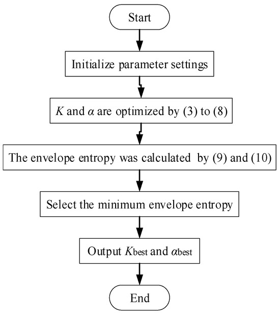
Figure 1.
Flow chart of the genetic particle swarm optimization algorithm.
2.3. Signal Denoising Based on VMD
White noise is the main noise source in the power system, due to the frequency distribution characteristics of power signals. Improving VMD decomposition, the low-frequency modal component is mainly composed of the dominant harmonic component. The low-frequency harmonic component has a high signal-to-noise ratio, but there are still a few noise components distributed in the whole frequency band. In the middle and high frequency modal component, the high-order harmonic content is low, the amplitude is small, and the signal is straightforward to be submerged by noise. As the signal-to-noise ratio is very low, noise has a great impact on the detection accuracy. Based on the above analysis, it can be seen that the effective signals in the middle and high frequency modes have limited influence on the accuracy of the analysis of broadband oscillation signals. The high noise content in the high frequency modes is prone to excessive order determination in the solution of Prony. Therefore, the middle and high frequency mode components can be regarded as noise components. Based on the above discussion, this paper proposes a denoising method based on energy threshold. According to the distribution of signal and noise in different frequency bands, the energy threshold is set, and the modal components with different energy levels are retained and screened to achieve a better denoising effect [31].
Considering the EMD, it is easy to lose part of the effective harmonic component in the signal, and all the noise in the high frequency band cannot be completely screened out. Therefore, the energy threshold method is adopted for denoising. That is, the decomposed modal components have different levels of energy, the IMF with larger energy a is harmonic component, and the IMF with smaller energy is a noise component and false component. By setting the threshold, the modal components that only contain noise in the signal are screened out.
where K is number of modal components, ui, ci are the modal component and its maximum value, respectively, c is the set of maximum values of each modal component, mi is the coefficient of energy. Threshold g needs to be set according to the noise content of the signal. If mi is less than g, the corresponding modal component is retained. Otherwise, the mode is regarded as noise and screened out.
3. Prony Algorithm and Evaluation Parameters
3.1. Prony Algorithm
Prony algorithm is a mathematical model based on a linear combination of exponential functions, which can achieve the fitting of signal with the same sampling interval and obtain the signal amplitude, frequency, phase and damping factor. According to Euler’s formula, the signal with sinusoidal component x(t) is converted into N equally spaced sampling points, written as:
where Ak is amplitude, fk is frequency, θk is phase, αk is damping factor, P is order of model, N is sampling number, Δt is sample interval, is signal of fit.
Equation (17) is the objective function of the minimum fitting error.
We constructed a linear difference equation with a constant coefficient, in which Equation (14) is the homogeneous solution and Equation (17) is the fitting error objective function.
where is error of fitting.
Taking error as the excitation of P-order autoregressive model , and achieving the actual signal x(n) to solve the regular equation. Hence, getting the parameter . Substitute into (20) and source the root of it to find the parameter zk.
According to Equation (14), the matrix equation is
In combination with the matrix equation of Equation (21), the parameter is obtained based on the idea of the least square method,
Finally, the amplitude, frequency, initial phase and damping factor of each component are obtained by , .
3.2. Order of Model
The model order of the Prony algorithm can reflect the number of harmonic components in the system. The closer the order is to the number of harmonic components, the higher the performance of the Prony algorithm and the better the fitting effect; SNR can reflect the noise content of the signal and the fitting degree of the Prony algorithm. The noise content of a signal is inversely proportional to the SNR. Therefore, the model order and signal-to-noise ratio are selected as the evaluation parameters of the algorithm performance.
The traditional model order selection methods generally include a singular value method of autoregressive model and an empirical method based on the number of sampling points, etc. In this paper, the model order selection method with SNR and mean square error as indicators is adopted. SNR can represent the fitting effect of the signal. When the order of the selected model approaches the real value of the system, SNR will increase. According to the experimental results, when SNR < 20 dB, the signal fitting effect is poor. When SNR > 50 dB, the signal can be accurately fitted [31]. In addition, the mean square deviation can reflect the change degree of SNR, when the SNR finally tends to be stable, the signal fitting is accurate.
4. Flow of Broadband Oscillation Mode Identification Algorithm
The identification accuracy and algorithm performance of the traditional Prony algorithm are greatly affected by noise, and the fitting effect of signals with low SNR is poor, resulting in the failure to accurately identify the characteristic parameters of signals. In addition, it is difficult to select the optimal decomposition parameters of the VMD decomposition algorithm, which can lead to the unsatisfactory signal decomposition effect and, ultimately, affect the signal denoising effect. Therefore, this paper adopts a new method combining particle swarm optimization (PSO), VMD and the Prony algorithm to analyze harmonic signals. The basic steps are as follows:
Step 1: The number of modes K and damping factor α, which have great influence on VMD decomposition, are optimized by the optimization algorithm to achieve the best effect of VMD decomposition.
Step 2: The optimal number of modes and damping factors obtained in step 1 are substituted into VMD decomposition, and the original signal is decomposed to obtain a series of modal components with different frequency bands.
Step 3: Combined with the idea of energy threshold method, the energy coefficient of each modal component is calculated, and the threshold value g is set for comparative analysis. The modal component containing only medium and high frequency noise is screened out.
Step 4: The real harmonic components are reconstructed, and the Prony algorithm is used to identify the reconstructed signal, and the amplitude, frequency, phase and damping factor of the signal are obtained.
Finally, the broadband oscillation mode is analyzed according to the obtained parameters. The flow chart is shown in Figure 2.
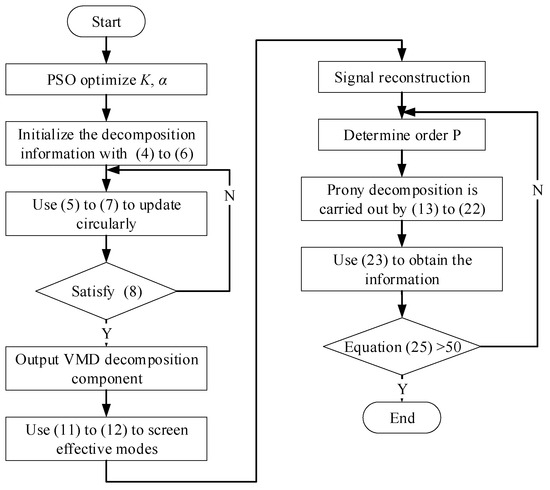
Figure 2.
Flow chart of the harmonic detection method.
5. Examples Analysis
In order to test the effectiveness of the proposed method for broadband oscillation mode identification, an electric power signal containing fundamental waves, harmonics and inter-harmonics is constructed in this paper.
The sampling frequency is set as 1000 Hz, and the number of sampling points is 500. The wave forms of the four groups of signals with noise and the noiseless signals are shown in Figure 3.
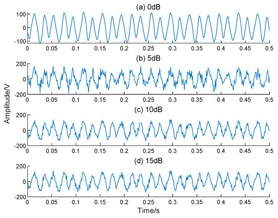
Figure 3.
Waveform of the noisy signal and the noiseless signal.
5.1. Analysis of Denoising Performance
In order to improve the decomposition effect of the VMD algorithm, distinguish effective signals from noise and false components, an optimization algorithm (PSO) is used to optimize the VMD decomposition parameters. It improves the performance of the Prony algorithm. First, set the initial parameters of the particle swarm optimization algorithm, including acceleration factor c1 and c2 are 1.8, the position interval of damping factor α is (1000, 8000), number of modes K position interval is (2, 8).
The particles were iterative updated according to the above parameters, and the envelope entropy was used as the fitness function. The optimal positions of particles under different noise levels are shown in Table 1.

Table 1.
Parameter values for different noise levels.
From Table 1, the number of modes K remains at 5 under different noise levels, but the value of the damping factor is inconsistent. Thus, the noise affects the value of the penalty factor while the number of modes K is not sensitive to noise.
Then, we chose the data with 15 dB noise added for subsequent analysis. The optimal number of modes and damping factors are substituted into the VMD algorithm to decompose the waveform and spectrum of each mode, as shown in Figure 4 and Figure 5.
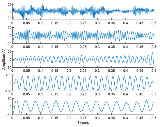
Figure 4.
Waveform of the signal with 15 dB noise.
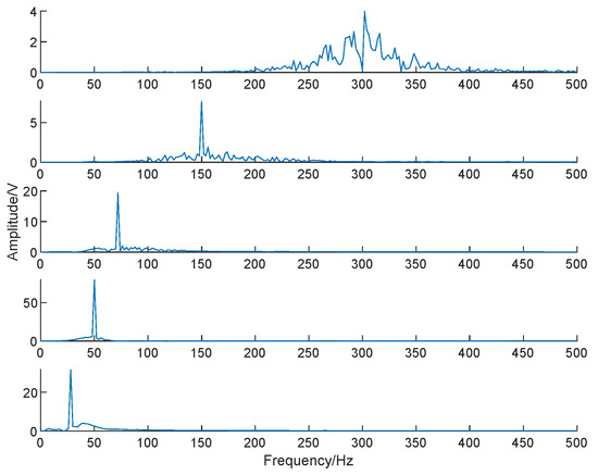
Figure 5.
FFT analysis of the signal with 15 dB noise.
According to Figure 4 and Figure 5, VMD decomposition can accurately obtain the amplitude and frequency of the modal component. Equations (11) and (12) calculate the energy level of each modal component and the results are shown in Table 2. Setting the threshold g is according to Table 2; IMF2~IMF5 are true harmonic components and they are retained for Prony analysis. It is concluded that the VMD decomposition method based on parameter optimization can accurately separate the effective component and noise component of the signal.
Table 2.
Energy coefficients for each modal component of the example signal.
5.2. Test Performance Analysis
In order to further verify the effectiveness and superiority of the proposed method in parameters identification, Prony identification is carried out on the signal reconstructed by VMD and the noiseless signal, respectively. Under different noise contents, when the fitted SNR is stable, the results of each fitted SNR are shown in Table 3. As can be seen from Table 3, the proposed method in this paper always has a stable SNR of de-noising fitting under different noise content, and the de-noising fitting effect shows a steady growth trend, indicating its robustness.
Table 3.
Fitting SNR under different noise content.
The result of different fitting orders for the signal with 15 dB noise added is shown in Figure 4. From Figure 6, the fitting effect of the proposed method is obviously better than that of Prony. The fitting SNR value of the proposed method is stable near 25.5 dB with Prony stable near 20 dB. It is proved that the proposed VMD based on particle swarm denoising is effective and can significantly improve the fitting effect of Prony.
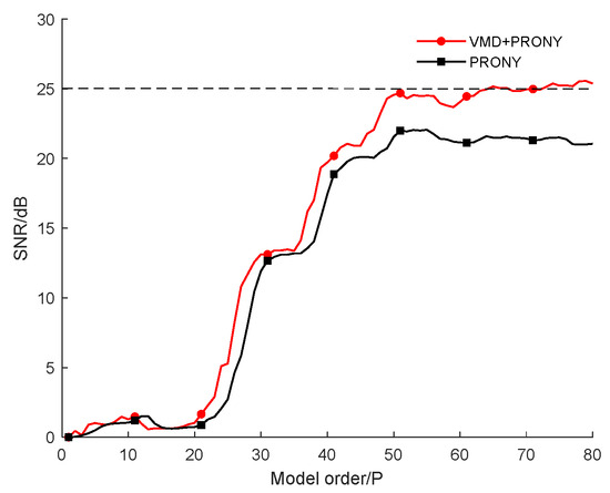
Figure 6.
Comparison of fitting effect of example signal.
When the model order is 75, the fitting SNR of VMD + Prony is 25.5475 dB, and the fitting SNR of Prony is 20.9977 dB. The identification results of specific parameters are shown in Table 4.
Table 4.
Identification result based on three methods from example data.
From Table 4, it can be seen that the average identification errors of amplitude and frequency of the proposed method are 4.4034% and 0.0291%, that of Prony is 7.1808% and 0.0827% and that of EMD+FFT is 5.9997% and 0. The identification results of the proposed method are better than Prony in amplitude and frequency, except the frequency of EMD+FFT. The identification errors in phasor and damping factor are smaller than Prony. Although EMD+FFT has a better frequency identification effect than the proposed method and Prony, the amplitude identification effect is worse than the proposed method due to the existence of the damping factor, and the damping factor cannot be obtained.
6. Simulation Analysis
In order to further verify the superiority of the algorithm, a system model with fan was built on the simulation platform in this paper. The simplified model is shown in Figure 7 below:
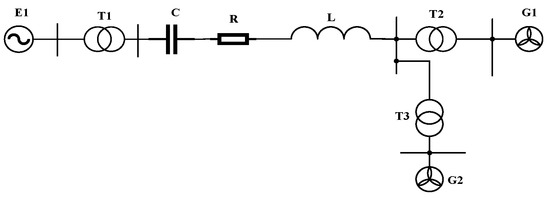
Figure 7.
This is a figure. Simplified model diagram with wind power generation. E1 represents equivalent system, G1 and G2 represent wind turbines, and L, R and C represent transmission line parameters.
The simulation data of voltage, current and function of broadband oscillation are obtained by running the simulation model. The voltage waveform obtained by simulation is shown in Figure 8, where the sampling frequency is 500 Hz and the sampling time is 0.4 s.
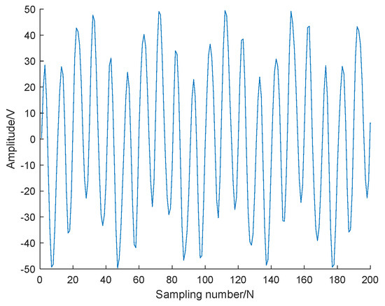
Figure 8.
Waveform of the signal.
Fourier transform is applied to this set of data to obtain the amplitude and frequency of this set of signals. The signal waveform and FFT analysis results are shown in Figure 9, and the identification results are shown in Table 5.
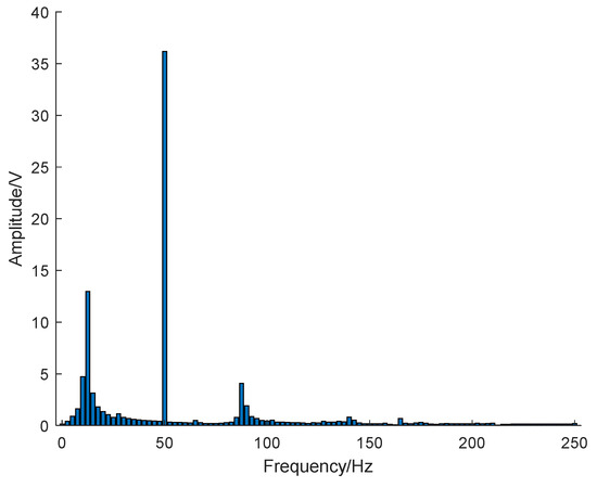
Figure 9.
FFT analysis spectrum of the signal.
Table 5.
FFT Analysis of the Signal Example.
6.1. Analysis of Denoising Performance
For the simulation signals, this paper changed the position interval of the number of modes to [2,5], which can ensure the accuracy of VMD decomposition results. The position interval of punishment factor is (1000, 8000), with other parameters unchanged. The optimal position of the particle is (5, 6819.1); it was substituted into the VMD algorithm. The decomposition results are shown in Figure 10 and Figure 11.
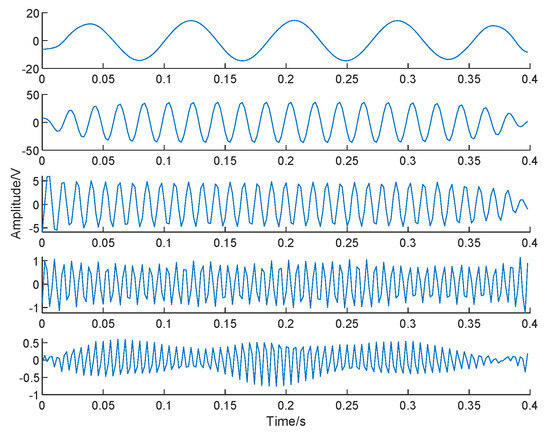
Figure 10.
Intrinsic Mode Functions waveform.
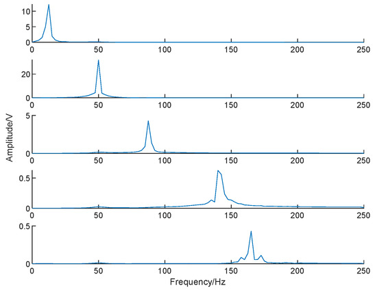
Figure 11.
Intrinsic Mode Functions spectrum.
According to Figure 10 and Figure 11, IMF1~IMF3 are true harmonic components and are retained for Prony analysis. It is concluded that the VMD decomposition method based on parameter optimization can accurately separate the effective component and noise component of the signal. The energy coefficients of each component are shown in Table 6.
Table 6.
Energy coefficients for each modal component of the simulation signal.
In order to test the denoising effect of the method presented in this paper, SNR and root mean square error (RMSE) are used as evaluation indexes in Table 7. SNR reflects the noise content in the signal. The denoising effect is proportional to the SNR. RMSE reflects the restoration degree of the denoised signal. RMSE decreases as the deviation between the denoised signal and the noiseless original signal decreases.
Table 7.
Denoising effect of different algorithms.
According to the evaluation index results in Table 8, the denoising ability of db2 wavelet hard threshold method and the method in this paper is compared and analyzed. It can be seen that the denoising effect of the proposed method is better than that of the db2 wavelet hard threshold method in terms of SNR and RMSE.
Table 8.
The fitting effect of different algorithms.
6.2. Test Performance Analysis
After signal reconstruction, in order to verify the effectiveness of the proposed method, the Prony algorithm is used to carry out signal fitting and harmonic identification for the original signal and reconstructed signal, respectively. The fitting effect is shown in Figure 12.
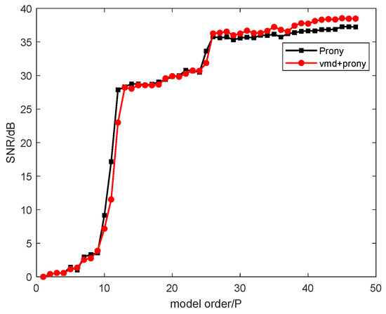
Figure 12.
Comparison of fitting effect of simulated signal.
As can be seen from Figure 12, the trend of the two curves is almost the same, indicating that the proposed method and the original Prony method have almost the same data processing capability. This is because Figure 12 analyzes the simulated signal, and no artificial noise is added, so the noise content of the final signal is very low, which can also be seen from Figure 9.
Under the condition of the same model order, the SNR results obtained by Prony analysis of different signals are shown in Table 8. The fitting SNR of reconstructed signal is 38.4783 dB, which is optimal. Under the condition that the model order is 47, the reconstructed signal and the original signal and the results denoised by the db2 wavelet hard threshold are identified. Results of identification are shown in Table 9.
Table 9.
Identification results based on three methods for simulation data.
It can be seen that the frequency and amplitude identification errors of the EMD+FFT are almost the same as those of the traditional Prony algorithm. However, the frequency and amplitude identification errors of the proposed method are smaller than those of the EMD+FFT and the traditional Prony algorithm. This method has the highest accuracy in harmonic identification.
Through the above simulation analysis of broadband oscillation, it can be seen that:
- (1)
- Based on time-domain analysis, the Prony algorithm cannot only obtain the frequency and amplitude obtained by FFT transformation, but can also obtain time-domain information such as the damping factor;
- (2)
- The VMD-Prony algorithm, proposed in this paper, is more accurate than EMD+FFT and the traditional Prony method. The effectiveness of the proposed algorithm is verified by comparing it with the traditional Prony algorithm.
In summary, the proposed method can obtain more time domain analysis results than FFT, such as the damping factor. Compared with the traditional Prony algorithm, the proposed method uses VMD denoising to solve the problem that the model order is too large, so that the identification accuracy is less affected by the model order. VMD denoising is better than the Kalman filter to solve the problem of insufficient precision of a nonlinear model. The denoising effect based on VMD is better than that based on EMD+FFT. The proposed method significantly reduces the influence of noise on signal identification. Therefore, the method in this paper is superior in engineering practicability.
7. Conclusions
It is prone to induce widebroad oscillation when new energy with high permeability is connected to a weak regional power grid. The accurate identification of the wide-frequency oscillation mode is the prerequisite to solve the resonant operation risk of new energy station. This paper proposes a new method for wind farm wide-band oscillation mode identification based on the combination of VMD and Prony, and focuses on the parameter optimization, noise removal and performance detection of VMD in the algorithm. The research conclusions are as follows:
- (1)
- The number of modes K and penalty factor α in the VMD algorithm have great influence on the algorithm, which can be augmented by particle swarm optimization.
- (2)
- Noise signals in measured data are likely to lead to poor analysis effect of the Prony algorithm. In this paper, a method combining the VMD algorithm and the energy threshold idea is adopted to effectively eliminate noise interference in data and retain effective components in signals.
- (3)
- In this paper, SNR and RMSE are used as evaluation indexes. The SNR reflects the size of noise content in a signal. The denoising effect is better with the increase in SNR. The RMSE reflects the restoration degree of the denoised signal. The smaller the RMSE, the smaller the deviation between the denoised signal and the noiseless original signal. In order to obtain accurate identification results, SNR is usually required to be greater than 20 dB.
The composition and distribution of noise are more complex in the actual environment, so further research on noise identification and removal for measured analysis can be carried out in the future. Furthermore, in Prony detection, when the fitting order is half of the number of sampled data points, the fitted SNR sudden drop phenomenon is still unclear, and the specific mechanism can be further studied in the next research.
Author Contributions
Conceptualization, C.G. and L.Y.; methodology, C.G., L.Y., B.C. and J.D. (Jianbo Dai); writing—original draft preparation, C.G. and L.Y.; writing—review and editing, J.D. (Jing Dai) and K.Y. All authors have read and agreed to the published version of the manuscript.
Funding
This research was funded by the National Natural Science Foundation of China (52367002) and Yunnan Province joint fund key project (202201BE070001-15).
Data Availability Statement
The raw/processed data required to reproduce these findings are contained within the article.
Acknowledgments
We would like to express our sincere gratitude to Kunming University of Science and Technology for their support.
Conflicts of Interest
Author Ke Yin was employed by the company Beijing Xinleineng Technology Co., Ltd., Chengdu Branch. The remaining authors declare that the research was conducted in the absence of any commercial or financial relationships that could be construed as a potential conflict of interest.
References
- Bai, J.; Xin, S.; Liu, J.; Zheng, K. Roadmap of Realizing the High Penetration Renewable Energy in China. Proc. CSEE 2015, 35, 14. [Google Scholar]
- Xie, X.; Liu, H.; He, J.; Liu, H.; Liu, W. On New Oscillation Issues of Power Systems. Proc. CSEE 2018, 38, 10. [Google Scholar]
- Chen, G.; Li, M.; Xu, T.; Liu, M. Study on Technical Bottleneck of New Energy Development. Proc. CSEE 2017, 37, 1. [Google Scholar]
- Ma, N.; Xie, X.; Tang, J.; Chen, L. Wide-area measurement and early warning system for wide-band oscillation in “double-high” power systems. J. Tsinghua Univ. (Sci. Technol.) 2021, 61, 5. [Google Scholar]
- Zhang, D.; Wang, Y.; Hu, J.; Ma, S.; He, Q.; Guo, Q. Impacts of PLL on the DFIG-based WTG’s electromechanical response under transient conditions: Analysis and modeling. CSEE J. Power Energy Syst. 2016, 2, 30–39. [Google Scholar] [CrossRef]
- Tong, Y.; Yin, Y. Multi-Scale Simulation and Test Technology of Power System; China Electric Power Press: Beijing, China, 2013; pp. 184–188. [Google Scholar]
- Ma, N.; Xie, X.; Kang, P.; Zhang, F. Wide-area Monitoring and Analysis of Subsynchronous Oscillation in Power Systems With High-penetration of Wind Power. Proc. CSEE 2021, 41, 1. [Google Scholar]
- Ma, N.; Xie, X.; He, J.; Wang, H. Review of broadband Oscillation in Renewable and Power Electronics Highly Integrated Power Systems. Proc. CSEE 2020, 40, 15. [Google Scholar]
- Wang, W.; Zhu, Y.; Liu, C.; Dong, P.; Hu, T.; Li, B.; Li, Y.; He, F.; Zhang, Y. Realization of Electromagnetic Real-time Simulation of Large-scale Grid Based on HYPERSIM. Power Syst. Technol. 2019, 43, 4. [Google Scholar]
- Zhang, F.; Cheng, L.; Gao, W.; Huang, R. Synchrophasors-based identification for subsynchronous oscillations in power systems. IEEE Trans. Smart Grid 2018, 10, 2224–2233. [Google Scholar] [CrossRef]
- Yang, X.; Zhang, J.; Xie, X.; Xiao, X.; Gao, B.; Wang, Y. Interpolated DFT-based identification of sub-synchronous oscillation parameters using synchrophasor data. IEEE Trans. Smart Grid 2019, 11, 2662–2675. [Google Scholar] [CrossRef]
- Xu, Y.; Liu, H.; Cheng, Y. Key Influencing Factors on Propagation of Sub-Synchronous Oscillations in AC and DC Grids. Mod. Electr. Power 2022, 1–11. [Google Scholar] [CrossRef]
- Mortensen, A.N.; Johnson, G.L. A power system digital harmonic analyzer. IEEE Trans. Instrum. Meas. 1988, 37, 537–540. [Google Scholar] [CrossRef]
- Yu, Y.; Zhao, W.; Li, S.; Huang, S. A Two-Stage Wavelet Decomposition Method for Instantaneous Power Quality Indices Estimation Considering Interharmonics and Transient Disturbances. IEEE Trans. Instrum. Meas. 2021, 70, 9001813. [Google Scholar] [CrossRef]
- Dragomiretskiy, K.; Zosso, D. Variational Mode Decomposition. IEEE Trans. Signal Process. 2014, 62, 531–544. [Google Scholar] [CrossRef]
- Riaz, F.; Hassan, A.; Rehman, S.; Niazi, I.K.; Dremstrup, K. EMD-Based Temporal and Spectral Features for the Classification of EEG Signals Using Supervised Learning. IEEE Trans. Neural Syst. Rehabil. Eng. 2016, 24, 28–35. [Google Scholar] [CrossRef] [PubMed]
- Laila, D.S.; Messina, A.R.; Pal, B.C. A Refined Hilbert–Huang Transform with Applications to Interarea Oscillation Monitoring. IEEE Trans. Power Syst. 2009, 24, 610–620. [Google Scholar] [CrossRef]
- Chen, K.; Jin, T.; Mohamed, M.A.; Wang, M. An Adaptive TLS-ESPRIT Algorithm Based on an S-G Filter for Analysis of Low Frequency Oscillation in Wide Area Measurement Systems. IEEE Access 2019, 7, 47644–47654. [Google Scholar] [CrossRef]
- Feng, S.; Cui, H.; Chen, J.; Tang, Y.; Lei, J. Applications and Challenges of Artificial Intelligence in Power System broadband Oscillation. Proc. CSEE 2021, 41, 23. [Google Scholar]
- Mo, W.; Lv, J.; Pawlak, M.; Annakkage, U.D.; Chen, H. Power System Oscillation Mode Prediction Based on the Lasso Method. IEEE Access 2020, 8, 101068–101078. [Google Scholar] [CrossRef]
- He, J.; Luo, G.; Cheng, M.; Liu, Y.; Tan, Y.; Li, M. A Research Review on Application of Artificial Intelligence in Power System Fault Analysis and Location. Proc. CSEE 2020, 40, 17. [Google Scholar]
- Ding, R.; Shen, Z. Modal Identification of Low-frequency Oscillation in Power System based on EMO-EDSNN. Autom. Electr. Power Syst. 2020, 44, 122–131. [Google Scholar]
- Gupta, A.K.; Verma, K. PMU-ANN based real timemonitoring of power system electromechanical oscillations. In Proceedings of the 2016 IEEE 1st International Conference on Power Electronics, Intelligent Control and Energy Systems (ICPEICES), Delhi, India, 4–6 July 2016; pp. 1–6. [Google Scholar]
- Chen, C.I.; Chang, G.W. Virtual instrumentation and educational platform for time-varying harmonics and interharmonics detection. IEEE Trans. Ind. Electron. 2010, 57, 3334–3342. [Google Scholar] [CrossRef]
- Hauer, F. Application of Prony analysis to the determination of modal content and equivalent models for measured power system response. IEEE Trans. Power Syst. 1991, 6, 1062–1068. [Google Scholar] [CrossRef]
- Pantaleon, C.; Souto, A. Comments on “An aperiodic phenomenon of the extended Kalman filter in filtering noisy chaotic signals”. IEEE Trans. Signal Process. 2005, 53, 383–384. [Google Scholar] [CrossRef]
- Smith, C.B.; Agaian, S.; Akopian, D. A Wavelet-Denoising Approach Using Polynomial Threshold Operators. IEEE Signal Process. Lett. 2008, 15, 906–909. [Google Scholar] [CrossRef]
- Janik, P.; Rezmer, J.; Ruczewski, P.; Waclawek, Z.; Lobos, T. Adaptation of SVD and Prony method for precise computation of current components in networks with wind generation. In Proceedings of the 2009 International Conference on Clean Electrical Power, Capri, Italy, 9–11 June 2009; pp. 624–629. [Google Scholar] [CrossRef]
- Li, Y.; Liang, X.; Yang, Y.; Xu, M.; Huang, W. Early Fault Diagnosis of Rotating Machinery by Combining Differential Rational Spline-Based LMD and K–L Divergence. IEEE Trans. Instrum. Meas. 2017, 66, 3077–3090. [Google Scholar] [CrossRef]
- Wang, R.; Huang, W.; Hu, B.; Du, Q.; Guo, X. Harmonic Detection for Active Power Filter Based on Two-Step Improved EEMD. IEEE Trans. Instrum. Meas. 2022, 71, 9001510. [Google Scholar] [CrossRef]
- Zhang, Z.; Tan, Z.; Zhang, C.; Wang, X.; Liu, X.; Yu, Y. Speech Endpoint Detection Based on Bayseian Decision of Logarithmic Power Spectrum Ratio in High and Low Frequency Band. Comput. Sci. 2021, 48, 6A. [Google Scholar]


Disclaimer/Publisher’s Note: The statements, opinions and data contained in all publications are solely those of the individual author(s) and contributor(s) and not of MDPI and/or the editor(s). MDPI and/or the editor(s) disclaim responsibility for any injury to people or property resulting from any ideas, methods, instructions or products referred to in the content. |
© 2024 by the authors. Licensee MDPI, Basel, Switzerland. This article is an open access article distributed under the terms and conditions of the Creative Commons Attribution (CC BY) license (https://creativecommons.org/licenses/by/4.0/).