Indeterminate Stieltjes Moment Problem: Entropy Convergence

Abstract

The aim of this paper is to consider the indeterminate Stieltjes moment problem together with all its probability density functions that have the positive real or the entire real axis as support. As a consequence of the concavity of the entropy function in both cases, there is one such density that has the largest entropy: we call it $f_{\mathrm{hmax}}$, the largest entropy density. We will prove that the Jaynes maximum entropy density (MaxEnt), constrained by an increasing number of integer moments, converges in entropy to the largest entropy density $f_{\mathrm{hmax}}$. Note that this kind of convergence implies convergence almost everywhere, with remarkable consequences in real applications in terms of the reliability of the results obtained by the MaxEnt approximation of the underlying unknown distribution, both for the determinate and the indeterminate case.

1. Introduction

For an absolutely continuous random variable X with the entire real axis as support and the associated Hamburger moment problem determinate, [1]—Thm.1 and [2] proved that the MaxEnt approximation converges in entropy to the unknown density f of X. Well-known necessary and sufficient conditions for the determinacy of the moment problem, as well as their geometric implications, were used to prove the above convergence result. In the present work, our goals consist of the following:

• improve the proof of convergence in entropy provided by [1], Section 3, when the Stieltjes moment problem is determinate, listing through the use of the limit parabolic regions described below all the possible cases that may arise;
• state and prove an analogous entropy convergence result in the case of the indeterminate Stieltjes moment problem. That extension is not immediate and additional considerations of MaxEnt distribution properties are required.

An enormous amount of material is available in the literature on the topic of the indeterminate moment problem, which has been extensively treated in the last and present centuries, employing different techniques of investigation. However, we will address this topic through a novel approach based on the notion of differential entropy and Jaynes’ MaxEnt techniques ([3]). More specifically, well-known necessary and sufficient conditions for Stieltjes moment problem determinacy/indeterminacy in terms of Hankel matrix determinants will be employed.

Such necessary and sufficient conditions, formulated through Theorems 3 and 4 below, have an interesting and enlightening geometric meaning. As a consequence, they will enable us to introduce and then exploit the notion of limit parabolic regions as a graphical tool for an easy and immediate understanding of such determinacy/indeterminacy conditions. Next, we will use these tools to prove the convergence in entropy of the MaxEnt solution of the indeterminate Stieltjes moment problem, which is the main result of the present paper.

There are several motivations to study the convergence in entropy of ${\left\{f_M\right\}}_{M=1}^{\infty }$ to $f_{\mathrm{hmax}}$, the density with the largest entropy among those sharing the given integer moment sequence ${\left\{{\mu }_k\right\}}_{k=1}^{\infty }$, ${\mu }_0=1$.

The original contribution of this paper is to exploit one of the characteristic properties of Shannon entropy; namely, that it is a concave functional.

Let ${\mathcal{C}}_{\infty }$ denote the infinite set of densities f, which are the solutions of the moment problem. It is noteworthy that in an M-infinite problem, by virtue of its concavity, the Shannon entropy induces an ordering principle in terms of entropy for the elements of ${\mathcal{C}}_{\infty }$: this guarantees the existence of a unique $f_{\mathrm{hmax}}$, distinguishable from all other functions $f\in {\mathcal{C}}_{\infty }$ such that it can be considered the genuine (that is, the most non-committal in Jaynes’ spirit) MaxEnt representative of all densities in ${\mathcal{C}}_{\infty }$. At the same time, it makes $f_{\mathrm{hmax}}$ the candidate limit to which the MaxEnt approximations converge in entropy, analogously to what happens in the determinate case, where the maximum entropy approximations converge to the unique density compatible with the information carried by the sequence of moments ${\left\{{\mu }_k\right\}}_{k=0}^{\infty }$.

Consistent with our purposes, of all the densities, $f_{\mathrm{hmax}}$ is the most important because, when all known information is taken into account, the system with the largest entropy is the most likely state as it is the system in which the least amount of information has been defined ([4]).

Moreover, the convergence in entropy is a stronger mode of convergence, which in turn implies convergence in direct divergence, in ${\mathcal{L}}^1$, in probability and in distribution. This concatenation of convergence modes has been proved in the work by [5], Section 4.3, for the case of fractional moments. However, considering that both integer and fractional moments belong to the so-called Tchebycheff systems, these convergence modes can be extended to the case of integer moments. Combining the convergence theorem in entropy proved below with the fact that $f_{\mathrm{hmax}}$ has the largest entropy $H\left[f_{\mathrm{hmax}}\right]$, one could find reasonable answers to several questions. Here, we limit ourselves to mentioning the following two.

• Consider the so-called Stieltjes class $S_{{\mathbb{R}}^{+}}(f_0,h)$ ([6], Section 3) with a center at $f_0$ and perturbation function h defined as follows:

  $$S_{{\mathbb{R}}^{+}}(f_0,h)=S_{ϵ}\left(x\right)=:\{f_0\left(x\right)[1+ϵh\left(x\right)],x\in {\mathbb{R}}_{+},ϵ\in [-1,1]\}.$$

  (1)

  where $f_0\left(x\right)$, $x\in {\mathbb{R}}^{+}$ is a continuous probability density function, that is, $f_0=F^{\prime }$, where F is the distribution function of some random variable X and $h\left(x\right)$ is a non-identically zero continuous function, satisfying the condition $-1\le h\left(x\right)\le 1$, for all $x\in {\mathbb{R}}^{+}$. Then, $S_{{\mathbb{R}}^{+}}(f_0,h)$ is an infinite family of densities all sharing the same moment sequence as $f_0$ and obviously requires knowledge of both functions $f_0$ and h. The latter satisfies the infinite relations ${\int }_{{\mathbb{R}}^{+}}{x}^k{f}_0\left(x\right)h\left(x\right)dx=0$, con $k=1,2,\dots$. Usually, both $f_0$ and h are chosen by trial and error to satisfy (1). It is well-known that convergence in entropy implies convergence almost everywhere. Consequently, it makes sense to assume $f_0\equiv f_{\mathrm{hmax}}$ since it is distinguishable (hence, identifiable) from all densities in $C_{\infty }$. Recently, h has been obtained with a precise theoretical procedure by [7], Thm. 1.2, starting from $f_0$. Therefore, through the combination of the proposal to assume $f_0\equiv f_{\mathrm{hmax}}$ with the theoretical procedure of López-Garcia for the calculation of h, a complete theoretical program for the construction of Stieltjes classes solely using the given moment sequence is outlined.
  The originality of our study lies in the fact that, within the class of densities, we identify a particular one, $f_{\mathrm{hmax}}$, with the highest entropy $H\left[f_{\mathrm{hmax}}\right]$. This density is the limit of a sequence of MaxEnt densities with an increasing number of moments coinciding with the given one.
• In the so-called Method of Moments, [8], Section 6, p. 540–541, proved the following.

  Theorem 1 ([9]). Let $F_M$ and F be probability distributions supported on $\mathbb{R}$ with finite moments of all orders, which we denote by ${\mu }_k^{\left(M\right)}$ and ${\mu }_k$, respectively. If F is the only distribution with the moments ${\left\{{\mu }_k\right\}}_{k=1}^{\infty }$ and if ${lim}_{M\to \infty }{\mu }_k^{\left(M\right)}={\mu }_k$ for $k=1,2,\dots$, then the sequence ${\left\{F_M\right\}}_{M=1}^{\infty }$ converges in distribution to F; that is

  $$\underset{M\to \infty }{lim}{F}_M\left(x\right)=F\left(x\right)$$

  (2)

  at any point of continuity of $F\left(x\right)$.
  The uniqueness of $F\left(x\right)$ is assumed to be not only sufficient for the validity of the relation (2) (at any point of continuity) but also necessary. Theorem 7 below leads us to conjecture that the assumed moment problem determinacy condition, designed to guarantee convergence in distribution, could be sufficient but not necessary. This topic will be investigated in future research.

The paper is organized follows: Section 2 presents two crucial known results that state necessary and sufficient conditions for the existence and the determinacy of the Hamburger and Stieltjes moment problem solution in terms of Hankel matrices and their determinants; their geometrical meaning is clarified through the relationships between the elements that characterize the corresponding limit parabolic regions. Section 3 exploits these regions to reformulate the necessary and sufficient conditions for the indeterminacy of the Hamburger and Stieltjes moment problem, preparing the theoretical framework for the proof of the convergence in entropy of the MaxEnt solution in the Stieltjes indeterminate case given in Section 4. The conclusions follow in Section 5.

2. Moment Problem: Existence and Determinacy Conditions

Suppose $\Omega$ is a continuum, $(\Omega ,\mathcal{A})$ a measurable space and $\nu$ a probability measure defined on $\mathcal{A}$. Let X be a continuous real-valued random variable defined on the probability space $(\Omega ,\mathcal{A},\nu )$ with ${\mathcal{U}}_X\subseteq \mathbb{R}$ as support and an absolutely continuous distribution function F and suppose that all (positive) integer moments of the random variable X

$${\mu }_k=\mathbb{E}\left[X^k\right]={\int }_{{\mathcal{U}}_X}{x}^{k}dF\left(x\right),k=0,1,2,\dots ,{\mu }_0=1$$

exist (or, equivalently, are finite). If F is the unique distribution having the sequence ${\left\{{\mu }_k\right\}}_{k=1}^{\infty }$ as its moment sequence, then F is uniquely determined by its moments; that is, we say that F is M-determinate (M-det), and the same holds for $\nu$ because there is always a (probability) measure $\nu$ behind the sequence ${\left\{{\mu }_k\right\}}_{k=1}^{\infty }$. Otherwise, F is M-indeterminate (M-indet): in this case, there exists more than one distribution (potentially, an infinite number) sharing the same moment sequence ${\left\{{\mu }_k\right\}}_{k=1}^{\infty }$ and, consequently, F is not uniquely determined by its moments and the same conclusion holds for the probability measure $\nu$.

We use standard terminology and notations generally accepted in the moment problem framework: if ${\mathcal{U}}_X=\mathbb{R}$, we say ${\left\{{\mu }_k\right\}}_{k=1}^{\infty }$ is a Hamburger moment sequence, while if ${\mathcal{U}}_X={\mathbb{R}}^{+}$, ${\left\{{\mu }_k\right\}}_{k=1}^{\infty }$ is a Stieltjes moment sequence.

Books such as those by [8,10,11] and, more recently, [12] are widely known references on this topic and contain exhaustive details on the debate over and progress made in the moment problems for a century.

The following deep analytical and non-trivial result can be obtained (see [13] for references): for a real moment sequence ${\left\{{\mu }_k\right\}}_{k=1}^{\infty }$, we define the $(N+1)\times (N+1)$-Hankel matrices as follows:

$${\Delta }_N={\left[{\mu }_{i+j}\right]}_{i,j=0}^N\mathrm{a}\mathrm{n}\mathrm{d}{\Delta }_{N,p}={\left[{\mu }_{i+j+p}\right]}_{i,j=0}^N,p=1,2,3,4,N\in \mathbb{N}$$

(3)

where ${\Delta }_N$ is the basic Hankel matrix with ${\Delta }_0=\left[{\mu }_0\right]$, while ${\Delta }_{N,p},p=1,2,3,4,$ are the shifted Hankel matrices. More precisely, ${\Delta }_{N,1}={\left({\mu }_{i+j+1}\right)}_{i,j=0}^N$ is based on the shifted moment sequence $\{{\mu }_1,{\mu }_2,\dots \}$ generated by the measure ${\nu }_1$ with $\mathrm{d}{\nu }_1=x\mathrm{d}\nu$, while ${\Delta }_{N,2}={\left({\mu }_{i+j+2}\right)}_{i,j=0}^N$ is based on the shifted moment sequence $\{{\mu }_2,{\mu }_3,\dots \}$ generated by the measure ${\nu }_2$ with $\mathrm{d}{\nu }_2=x^2\mathrm{d}\nu$, and similarly for ${\Delta }_{N,3}$ and ${\Delta }_{N,4}$. This is similar to the case of the basic Hankel matrix, ${\Delta }_{0,p}=\left[{\mu }_p\right]$. Further, let

$$D_N:=\det {\Delta }_N=\mid {\Delta }_N\mid \mathrm{a}\mathrm{n}\mathrm{d}{D}_{N,p}:=\det {\Delta }_{N,p}=\mid {\Delta }_{N,p}\mid$$

(4)

be the determinants of the Hankel matrices, as defined in (3). It is a well-known fact that the positivity of the determinants (4) of all orders N is a necessary and sufficient condition for the existence of the moment problem solution. In other words, Hankel matrices (3) must be positive definite for all $N\in \mathbb{N}$.

The following theorem states a well-known result:

Theorem 2

(Fundamental Theorem [14]). Suppose that F is M-indet. Then, there are infinitely many absolutely continuous distributions and infinitely many purely discrete distributions, all of them sharing the same moments of F.

In what follows, since we need both to specify some special values of ${\mu }_0$ and ${\mu }_1$ and at the same time think ${\mu }_1$ as continuously varying, we will denote with ${\mu }_0^{*}$ and ${\mu }_1^{*}$ the values of ${\mu }_0$ and ${\mu }_1$ that have been preassigned.

The following Theorems 3 and 4, jointly with the geometric interpretation of the determinacy/indeterminacy conditions as developed by [15], allow us to draw the limit parabolic regions. They play a fundamental role for the aims of this paper as we will see in Section 4.2, where different determinate–indeterminate configurations of the Stieltjes moment problem (jointly with the Hamburger one) will be considered in terms of $({\mu }_0,{\mu }_1)$.

Theorem 3

([8], Thm. 2.18, p. 69). Let ν be a measure associated with the positive definite Hamburger moment sequence ${\left\{{\mu }_k\right\}}_{k=0}^{\infty }$. Then, ν is determinate if and only if at least one of the quantities $\frac{D_N}{D_{N-1,2}}$ and $\frac{D_{N-1,2}}{D_{N-2,4}}$ has a limit of zero as $N\to \infty$.

Theorem 3 has an interesting and enlightening geometric meaning. Consider the finite moment set ${\left\{{\mu }_k\right\}}_{k=0}^M$ with $M=2N$, where ${\mu }_0$ varies continuously whilst the remaining ones are kept fixed. The relationship

$$\frac{D_N}{D_{N-1,2}}={\mu }_0^{*}-{\mu }_{0,M}^{-}$$

(5)

holds, where ${\mu }_{0,M}^{-}$ comes from the equation $D_N\left({\mu }_{0,M}^{-}\right)=0$, replacing ${\mu }_0^{*}$ with ${\mu }_{0,M}^{-}$, so that the sequence ${\left\{{\mu }_{0,M}^{-}\right\}}_{M=2}^{\infty }$ is monotonic non-decreasing and, as $M\to \infty$, converges to a limit; say, ${\mu }_{0,\infty }^{-}={lim}_{M\to \infty }{\mu }_{0,M}^{-}\le {\mu }_0^{*}$. From Theorem 3, in the indeterminacy case,

$${\mu }_0^{*}-{\mu }_{0,\infty }^{-}>0.$$

(6)

holds. This inequality will be useful in what follows, when the limit parabolic regions are obtained. Similarly, consider once more ${\left\{{\mu }_k\right\}}_{k=0}^M$, where ${\mu }_1$ varies continuously whilst the remaining ones are kept fixed. If $D_N$, the determinant of the Hankel matrix ${\Delta }_N$, is regarded as a function of ${\mu }_1$, $D_N=D_N\left({\mu }_1\right)$ is a quadratic function with leading term $-D_{N-2,4}<0$, so that

$$\frac{D_N}{D_{N-2,4}}=-({\mu }_1^{*}-{\mu }_{1,M}^{+})({\mu }_1^{*}-{\mu }_{1,M}^{-})$$

(7)

where ${\mu }_{1,M}^{-}$ and ${\mu }_{1,M}^{+}$ are solutions of the equation $D_N\left({\mu }_{1,M}^{\pm }\right)=0$ with ${\mu }_{1,M}^{-}\le {\mu }_1^{*}\le {\mu }_{1,M}^{+}$. Since ${\Delta }_N$ is symmetric and positive definite, as M increases, ${\mu }_{1,M}^{-}$ is monotonically non-decreasing whilst ${\mu }_{1,M}^{+}$ is monotonically non-increasing, so that the intervals $[{\mu }_{1,M}^{-},{\mu }_{1,M}^{+}]$ for each value of M are nested. Combining Theorem 3 with Equation (7), it follows that

$$\frac{D_N}{D_{N-1,2}}·\frac{D_{N-1,2}}{D_{N-2,4}}=\frac{D_N}{D_{N-2,4}}=-({\mu }_1^{*}-{\mu }_{1,M}^{+})({\mu }_1^{*}-{\mu }_{1,M}^{-})$$

(8)

and, as a consequence, the determinacy/indeterminacy convergence conditions can be drawn. In the H-det case,

$$\underset{n\to \infty }{lim}{\mu }_{1,M}^{-}=\underset{n\to \infty }{lim}{\mu }_{1,M}^{+}={\mu }_1^{*}$$

(9)

while in the H-indet case,

$$\underset{M\to \infty }{lim}{\mu }_{1,M}^{-}<{\mu }_1^{*},\underset{M\to \infty }{lim}{\mu }_{1,M}^{+}>{\mu }_1^{*}$$

(10)

strictly. Equations (9) and (10) are the distinguishing features of the H-det and H-indet cases. At the end, they allow us to define the Hamburger moment problem determinacy or indeterminacy conditions only in terms of the differences ${\mu }_1^{*}-{\mu }_{1,\infty }^{-}$ or ${\mu }_{1,\infty }^{+}-{\mu }_1^{*}$. This aspect will play an important role in Section 3, in which the Stieltjes moment problem determinacy/indeterminacy is geometrically interpreted through the limit parabolic regions.

Theorem 4

([15], Lemma 3). Let ν be a measure associated with the positive definite Stieltjes moment sequence ${\left\{{\mu }_k\right\}}_{k=0}^{\infty }$. Then, ν is determinate if and only if at least one of the quantities $\frac{D_N}{D_{N-1,2}}$ and $\frac{D_{N,1}}{D_{N-1,3}}$ has a limit of zero as $n\to \infty$.

Theorem 4, like Theorem 3, has an interesting and enlightening geometric meaning (note that the quantity $\frac{D_N}{D_{N-1,2}}$ has been previously investigated in the Hamburger moment problem). As far as $\frac{D_{N,1}}{D_{N-1,3}}$ is concerned, consider the finite moment set ${\left\{{\mu }_k\right\}}_{k=1}^M$ with $M=2N+1$, where ${\mu }_1$ varies continuously whilst the remaining ones are kept fixed. The following relationship holds:

$$\frac{D_{N,1}}{D_{N-1,3}}={\mu }_1^{*}-{\mu }_{1,M}^{-}$$

(11)

where the number ${\mu }_{1,M}^{-}$ is the unique solution of the equation $D_{N,1}\left({\mu }_{1,M}^{-}\right)=0$ in which ${\mu }_1^{*}$ is replaced with ${\mu }_{1,M}^{-}$. The numerical sequence ${\left\{{\mu }_{1,M}^{-}\right\}}_{M=1}^{\infty }$ is monotonic non-decreasing and, as $M\to \infty$, convergent to a limit; say, ${\mu }_{1,\infty }^{-}\le {\mu }_1^{*}$. The indeterminacy condition is formulated as follows:

$${\mu }_1^{*}-{\mu }_{1,\infty }^{-}>0$$

(12)

In the end, Equations (6)–(12) allow us to define the Stieltjes moment problem determinacy or indeterminacy conditions only in terms of the difference ${\mu }_0^{*}-{\mu }_{0,\infty }^{-}$ and ${\mu }_1^{*}-{\mu }_{1,\infty }^{-}$ (the latter coming from (11) and (12)). This aspect will play an important role in Section 4 where convergence in entropy of the MaxEnt approximation (14) of f will be discussed in the S-indet case.

Notice that, in order not to burden the notation in the two Hamburger and Stieltjes cases, given the first M moments ${\left\{{\mu }_k\right\}}_{k=1}^M$, we denoted with the same symbol ${\mu }_{1,M}^{-}$ two quantities that are solutions of two distinct equations: in the Hamburger case, with $M=2N$, $D_N\left({\mu }_{1,M}^{-}\right)=0$; and in the Stieltjes case, with $M=2N$ or $M=2N+1$, $D_{N,1}\left({\mu }_{1,M}^{-}\right)=0$. We specify that, in the subsequent Stieltjes problem investigation, the values of ${\mu }_1^{*}-{\mu }_{1,M}^{-}$ will be drawn from (11) rather than from (7), in accordance with the next Theorem 6.

3. Limit Parabolic Regions

The limit parabolic regions represent an enlightening device for giving an intuitive graphical representation of the determinacy or indeterminacy conditions for the Stieltjes or Hamburger moment problems. In this paper, we are mostly interested in the indeterminacy condition.

1.

Hamburger case

Suppose ${\left\{{\mu }_k\right\}}_{k=0}^{\infty }$ is a moment sequence for which the moments $\{{\mu }_2,{\mu }_3,\dots \}$ are kept fixed while the moments ${\mu }_0$ and ${\mu }_1$ are left to be continuously varying. Setting $x={\mu }_0$ and $y={\mu }_1$, the whole moment sequence can be written as $\{x,y,{\mu }_2,{\mu }_3,\dots \}$ and the numbers x and y (i.e., the moments preceding ${\mu }_2$) cannot be arbitrary.

Following [15], we set $M=2N$ and consider the moments:

$$({\mu }_0,{\mu }_1,{\mu }_2,\dots ,{\mu }_M)=(x,y,{\mu }_2,\dots ,{\mu }_M)$$

where, as before, ${\mu }_2,\dots ,{\mu }_M$ are fixed and $x={\mu }_0$ and $y={\mu }_1$ can vary continuously. For each M, the relation $D_N(x,y)\ge 0$ defines a closed convex region as follows:

$${\mathcal{P}}_M:=\{(x,y)\in {\mathbb{R}}^2:D_N(x,y)\ge 0\}$$

(13)

which is bounded by a proper parabola with horizontal axis and vertex in the right-half plane. Since, for $M=1,2,\dots$, the Hankel matrices ${\Delta }_N(x,y)$ are positive semidefinite, the regions ${\mathcal{P}}_M$ are nested (i.e., ${\mathcal{P}}_M\subset {\mathcal{P}}_{M-1}$) and the element of interest is their intersection, $\mathcal{P}:={\bigcap }_{M=1}^{\infty }{\mathcal{P}}_M$, called a limit parabolic region. One possibility is that $\mathcal{P}$ is a proper closed region in the right-half plane such that $\mathcal{P}$ is bounded by a proper parabola and contains the initially given moments $({\mu }_0,{\mu }_1).$ The alternative is that $\mathcal{P}$ degenerates, becoming just a ray.

Theorem 5 ([15], Thm 1). Let ${\{x,y,{\mu }_k\}}_{k=2}^{\infty }$ be a Hamburger moment sequence for the measure ν. Then, ν is indeterminate if and only if the point $({\mu }_0^{*},{\mu }_1^{*})$ is an interior point of the limit parabolic region $\mathcal{P}$.

Theorem 5 is the geometric equivalent to the algebraic formulation of the Hamburger moment problem indeterminacy given in terms of Equations (6) and (10).

2.

Stieltjes case

Suppose that ${\left\{{\mu }_k\right\}}_{k=0}^{\infty }$ is a Stieltjes moment sequence. In this case, we develop a procedure similar to that in the Hamburger case but with some specific features. For doing this, we rely essentially on two known results. First, we recall that every Stieltjes sequence can also be considered a Hamburger sequence; hence, the existence of the limit parabolic region $\mathcal{P}$ is assured and defined by the two relations $D_N(x,y)\ge 0$ and $D_{N-1,1}\left(y\right)\ge 0$, in which we use $x={\mu }_0$ and $y={\mu }_1$. Second, $\mathcal{P}=\{(x,y):x\ge {\mu }_{0,\infty }^{-},y={\mu }_{1,\infty }^{-}\}$, a ray, or $\mathcal{P}$ is the intersection of proper limit parabolic regions in the half plain $\{y\ge {\mu }_{1,\infty }^{-}\}$. Taking into account Theorem 5, the following conclusion can be drawn.

Theorem 6 ([15], Thm 2). The positive definite Stieltjes moment sequence ${\left\{{\mu }_k\right\}}_{k=0}^{\infty }$ generates an indeterminate measure ν if and only if two conditions are satisfied:

(i) 

the point $({\mu }_0^{*},{\mu }_1^{*})$ is an interior point of the limit parabolic region $\mathcal{P}$;

(ii) 

${\mu }_{1,\infty }^{-}<{\mu }_1^{*}$.

Again, Theorem 6 is geometrically equivalent to the algebraic formulation of the Stieltjes moment problem indeterminacy given in terms of Equations (6), (11) and (12).

4. Stieltjes Moment Problem

The inverse moment problem consists of recovering the unknown PDF f knowing the sequence of its moments ${\left\{{\mu }_k\right\}}_{k=1}^{\infty }$ ([8]). For practical purposes, only a finite number M of moments ${\left\{{\mu }_k\right\}}_{k=1}^M$ is considered so that what we have is the so-called reduced (or truncated) moment problem, and it may have infinitely many solutions. Then, one needs a criterion for selecting the most appropriate probability density function among the available solutions. The strategy of selecting the least biased estimate of f can be based on the MaxEnt method ([3]).

4.1. Maxent Method

Given the first M moments ${\left\{{\mu }_k\right\}}_{k=1}^M$,

$$f_M\left(x\right)=exp\left(-\sum _{j=0}^M{\lambda }_j{x}^j\right)$$

(14)

provides the MaxEnt approximation ([16], p. 59) of f, supplemented by the $(M+1)$ conditions

$${\int }_{{\mathbb{R}}^{+}}{x}^k{f}_M\left(x\right)dx={\mu }_k,k=0,\dots ,M$$

and ${\mu }_0=1$, (14) being a density function with differential entropy (for short, entropy)

$$H\left[f_M\right]=-{\int }_{{\mathbb{R}}^{+}}{f}_M\left(x\right)ln{f}_M\left(x\right)dx=\sum _{k=0}^M{\lambda }_k{\mu }_k,$$

That is to say that $f_M$ has the largest entropy out of all densities sharing the first M moments with f. Note an important fact: the sequence ${\left\{H\left[f_M\right]\right\}}_{M=1}^{\infty }$ is monotonic non-increasing.

Let

$${\mathcal{C}}_{\infty }=:\left\{f\ge 0:{\int }_{{\mathbb{R}}^{+}}{x}^{k}f\left(x\right)dx={\mu }_k,k=1,2,\dots \right\}.$$

(15)

be a convex set of (density) functions that, in the M-indet case, include infinitely many densities, which are solutions of the moment problem. The class ${\mathcal{C}}_{\infty }$ will play a strategic role in the proof of the entropy convergence theorem. Since, as is well known, Shannon entropy possesses many good properties, one of which is to be a concave functional, a unique density—say, $f_{hmax}\in {\mathcal{C}}_{\infty }$—with the largest entropy exists, as shown by the following:

$$H\left[f_{hmax}\right]=\underset{f\in {\mathcal{C}}_{\infty }}{max}H\left[f\right].$$

After a brief revision of the S-det (with H-det) case, previously covered by [1], with the aim of giving a new and more structured interpretation of the determinacy conditions in terms of limit parabolic regions, our attention will be devoted to one of the central topics in this paper: a deep discussion of the S-indet case, the associated MaxEnt solution $f_M$ and the proof of convergence in entropy of $f_M$ to the underlying unknown density f.

4.2. Limit Parabolic Regions for S-Det or S-Indet

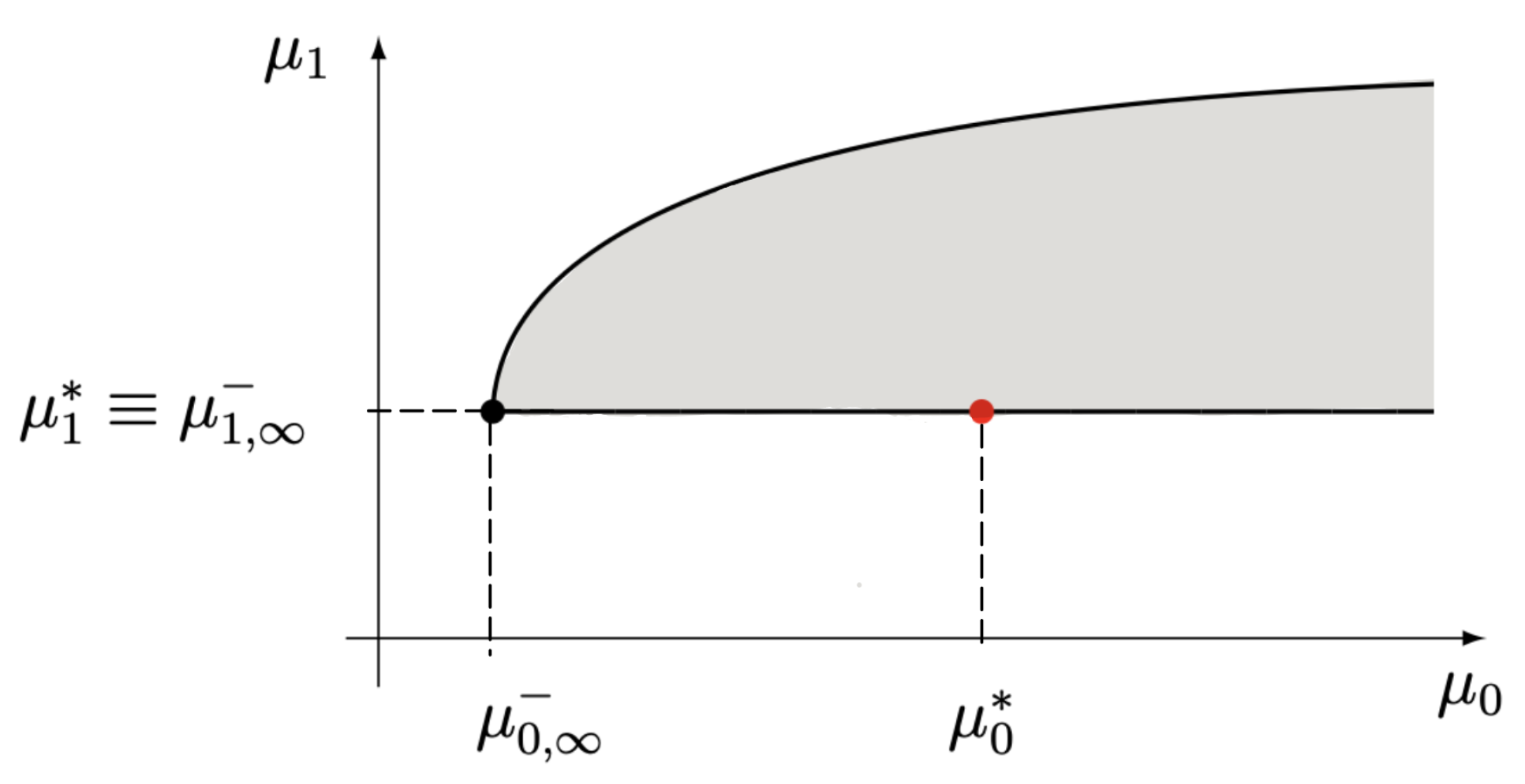
Let us summarize the known facts: an S-det measure $\nu$ may be either H-indet or H-det, while an S-indet measure $\nu$ is H-indet. Suppose that ${\left\{{\mu }_k\right\}}_{k=1}^M$, with $M=2N$, for instance, is a moment set. Thus, we have the following cases.

  Case 1:  

$\nu$ is S-det with H-indet (see [15], Corollary, p. 417). Combining Theorems 3 and 4, it follows that

$$\frac{D_N}{D_{N-1,2}}\to c_0>0\mathrm{and}\frac{D_{N,1}}{D_{N-1,3}}\to 0$$

equivalently, and both ${\mu }_{0,\infty }^{-}<{\mu }_0^{*}$ from (6) and ${\mu }_{1,\infty }^{-}={\mu }_1^{*}$ (see Figure 1).

Note that both here and in the following graphs, the shaded area represents the parabolic region and the red dot indicates the fixed value $({\mu }_0^{*},{\mu }_1^{*})$ of the point $({\mu }_0,{\mu }_1)$. Ref. [17], in a corollary on p. 481, states that if a measure $\nu$ is determinate in the Stieltjes sense and indeterminate in the Hamburger sense, then $\nu$ is a Nevanlinna-extremal measure and, in particular, is discrete with a positive mass at the origin. As a consequence, the S-det case is disregarded. In contrast, the H-indet case where infinitely many densities occur, will be investigated in Lemma (1).

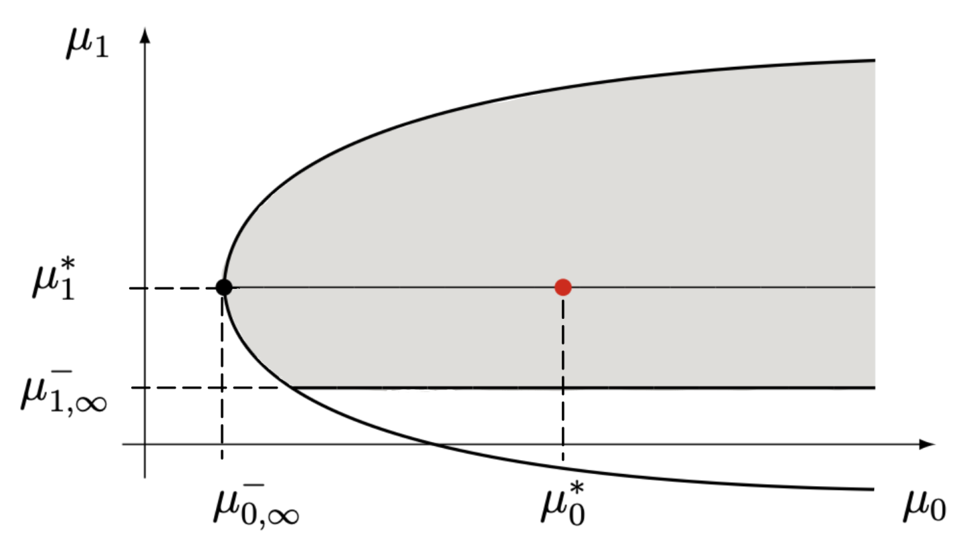
  Case 2:  

$\nu$ is S-indet with H-indet.

There are infinitely many densities with support ${\mathbb{R}}^{+}$ and $\mathbb{R}$. Combining Theorems 3 and 4, both inequalities ${\mu }_{0,\infty }^{-}<{\mu }_0^{*}$ and ${\mu }_{1,\infty }^{-}<{\mu }_1^{*}$ follow; equivalently, from Theorem 6, the point $({\mu }_0^{*},{\mu }_1^{*})$ is inside the limit parabolic (see Figure 2).

Entropy convergence in both cases S-indet and H-indet will be investigated below.

  Case 3. 

$\nu$ is S-det with H-det.

For a given moment sequence, S-det means that there is only one measure with support $[0,\infty )$ compatible with it. Here, we take the opportunity to review and refine the proof previously given by [1], Section 3. Combining Theorems 3 and 4 and their geometric meaning, we find that there are four possible limit parabolic regions, all of which are feasible. More specifically, we have the following:

(a)

the two limit parabolic regions degenerate into different rays, both arising from

$$\frac{D_{N-1,2}}{D_{N-2,4}}\to 0\mathrm{and}\frac{D_{N,1}}{D_{N-1,3}}\to 0$$

so that ${\mu }_{1,\infty }^{-}={\mu }_1^{*}$ and from

$$\frac{D_N}{D_{N-1,2}}\to 0\mathrm{or}\frac{D_N}{D_{N-1,2}}\to c_0>0,$$

respectively. Hence, ${\mu }_{0,\infty }^{-}={\mu }_0^{*}$ or ${\mu }_{0,\infty }^{-}<{\mu }_0^{*}$ occur;

(b)

a non-degenerate limit parabolic region arising from Case 1. Accordingly, we have S-det with H-indet after removing the mass at the origin, so that both

$$\frac{D_N}{D_{N-1,2}}\to 0\mathrm{and}\frac{D_{N,1}}{D_{N-1,3}}\to 0$$

(see Figure 3). In agreement with the results for S-det attained in Case 1, the measure is once more purely discrete with no mass at the origin and then it has to be disregarded;

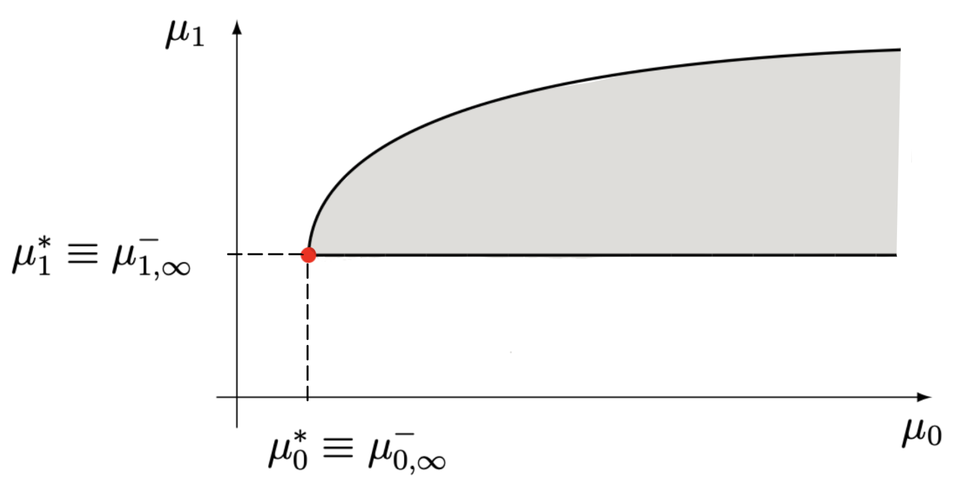
(c)

a non-degenerate limit parabolic region arising from the conditions

$$\frac{D_N}{D_{N-1,2}}\to 0\mathrm{and}\frac{D_{N,1}}{D_{N-1,3}}\to c_1$$

so that the corresponding distribution has zero mass at the origin. As a consequence ${\mu }_{0,\infty }^{-}={\mu }_0^{*}$ and ${\mu }_{1,\infty }^{-}<{\mu }_1^{*}$ hold, so that the point $({\mu }_0^{*},{\mu }_1^{*})$ is on the boundary of the limit parabolic region (see Figure 4).

The nature (probability mass or density) of the unique solution can now be investigated by adding a mass $\delta$ at the origin and renormalizing. The moments sequence amounts to ${\{1,{\mu }_k/(1+\delta )\}}_{k=1}^{\infty }$. In such a case, the moment problem becomes S-indet with H-indet (Figure 2), with maximum mass concentration $\frac{\delta }{1+\delta }$ at the origin. As is known, in an indeterminate Hamburger problem the maximum mass concentration at the origin just coincides with $\frac{\delta }{1+\delta }$, so that the initial solution is transformed into an extremal solution of the S-indet with H-indet problem. Since there exists only a discrete extremal solution of the moment problem for which this maximum is attained [8], Thm. 2.13, p. 60; [11], Corollary 7.17, p. 159), the original determinate Stieltjes solution is purely discrete with no mass at the origin, in accordance with with [18] p. 94. Thus, it has to be disregarded.

In conclusion, collecting together the just-above-limit parabolic regions (a), (b) and (c), it can be concluded that a necessary condition for a density to be associated with the unique measure S-det with H-det is that the corresponding limit parabolic region is degenerate, from which ${\mu }_{1,\infty }^{-}={\mu }_1^{*}$. Under the latter condition, the entropy convergence had been proved by [1], Section 3. Note that thanks to the MaxEnt formalism, the proof provided by the authors was completely analogous to the one used in the determinate Hamburger problem. Thus, the first goal outlined in the Introduction has been reached.

Regarding the proof of entropy convergence in the two cases S-indet and S-det, comparing Case 2 with Case 3, the crucial difference is due to the two distinct conditions ${\mu }_{1,\infty }^{-}<{\mu }_1^{*}$ and ${\mu }_{1,\infty }^{-}={\mu }_1^{*}$ that hold in the two cases, respectively. As a consequence, the proving procedure adopted for the S-det case (in which the relationship ${\mu }_{1,\infty }^{-}={\mu }_1^{*}$ plays a basic role) cannot be simply extended to the S-indet one. For the latter case, the entropy convergence is investigated below and represents the second main goal of this paper, as outlined in the Introduction.

4.3. Convergence in Entropy of the Maxent Approximation in the S-Indet Case

In analogy with the S-det case investigated by [1], Section 3, it is reasonable to conjecture that, in the S-indet case, the MaxEnt approximation $f_M$ also converges in entropy to the underlying unknown density $f_{hmax}$. Indeed, considering two distinct cases concerning the nature of the support of the density f (that is, ${\mathbb{R}}^{+}$ and $\mathbb{R}$) and relying in both cases on the fact that the sequence $\left\{H\left[f_M\right]\right\}$ is monotonically non-increasing with a finite lower bound $H\left[f_{hmax}\right]$, we can prove Theorems 7 and 8, the second two main results of this paper.

However, before presenting and proving these results, we briefly recall some basic steps of the convergence in entropy proof in the determinate Hamburger problem as given by [1], Thm. 1, and in the same paper also extended to the S-det case. The determinacy condition used for the Hamburger moment problem is given by (9). As we will see later, this procedure is the essential tool for proving entropy convergence in the S-indet case too.

1.

Let $\nu$ be the unique measure with support $\mathbb{R}$ and density f having the given moment sequence ${\left\{{\mu }_k\right\}}_{k=0}^{\infty }$. Consider the finite set ${\left\{{\mu }_k\right\}}_{k=1}^M$, with $M=2N$. If $({\mu }_0,{\mu }_2,\dots ,{\mu }_M)$ are kept fixed while ${\mu }_1\in ({\mu }_{1,M}^{-},{\mu }_1^{*}]$ varies continuously, the function $H\left[f_M\right]\left({\mu }_1\right)$ is monotonic increasing and concave (to ensure the monotonicity of $H\left[f_M\right]\left({\mu }_1\right)$, if needed, the interval ${\mu }_1\in ({\mu }_{1,M}^{-},{\mu }_1^{*}]$ could be replaced with $[{\mu }_1^{*},{\mu }_{1,M}^{+})$, leaving the procedure unchanged). As ${\mu }_1\to {\mu }_{1,M}^{-}$, $D_N\to 0$ so that $f_M$ corresponds to a purely discrete distribution with a finite number of mass points ([8], p. 5, Thm. 1.2). Then, as the differential entropy of a discrete distribution can be considered to be $-\infty$ ([4], p 247-9), ${lim}_{{\mu }_1\to {\mu }_{1,M}^{-}}H\left[f_M\right]\left({\mu }_1\right)=-\infty$ holds. On the other hand, as ${\mu }_1={\mu }_1^{*}$, $H\left[f_M\right]\left({\mu }_1^{*}\right)\ge H\left[f\right]$ holds. Then, since $H\left[f_M\right]\left({\mu }_1\right)$ is a continuous function of ${\mu }_1$, there exists a value of ${\mu }_1\in ({\mu }_{1,M}^{-},{\mu }_1^{*}]$ (say ${\xi }_M={\xi }_M(M,H\left[f\right])$) such that $H\left[f_M\right]\left({\xi }_M\right)=H\left[f\right]$. As $M\to \infty$, from ${lim}_{M\to \infty }{\mu }_{1,M}^{-}={\mu }_1^{*}$ (and then ${lim}_{M\to \infty }{\xi }_M={\mu }_1^{*}$ too) it follows that $H\left[f_M\right]\left({\xi }_M\right)=H\left[f_M\right]\left({\mu }_1^{*}\right)=H\left[f\right]$. From here, ${lim}_{M\to \infty }H\left[f_M\right]\left({\mu }_1^{*}\right)=H\left[f\right]$, which proves the entropy convergence in the H-det case.

2.

From Theorem 6, in the S-indet case, the point $({\mu }_0^{*},{\mu }_1^{*})$ is an interior point of the limit parabolic region such that ${\mu }_{1,\infty }^{-}<{\mu }_1^{*}$. In accordance with the above item in this list, $H\left[f_M\right]\left({\mu }_1\right)$ is monotonic increasing over ${\mu }_1\in ({\mu }_{1,M}^{-},{\mu }_1^{*}]$ with

$$\underset{{\mu }_1\to {\mu }_{1,M}^{-}}{lim}H\left[f_M\right]\left({\mu }_1\right)=-\infty \mathrm{and}H\left[f_M\right]\left({\mu }_1^{*}\right)\ge H\left[f_{hmax}\right].$$

As we have ${\mu }_{1,\infty }^{-}<{\mu }_1^{*}$, both scenarios are admissible as follows:

(i)

${lim}_{M\to \infty }H\left[f_M\right]>H\left[f_{hmax}\right]$ (strictly);

(ii)

${lim}_{M\to \infty }H\left[f_M\right]=H\left[f_{hmax}\right]$

Following the procedure outlined in the first item of this list, no conclusion about entropy convergence can be drawn, so an alternative approach must be sought.

4.3.1. Densities Supported on ${\mathbb{R}}^{+}$

Now we are ready to prove the first out the two main results of this paper.

Theorem 7 (Main result I). In the indeterminate Stieltjes problem, the MaxEnt approximate sequence ${\left\{f_M\right\}}_{M=1}^{\infty }$ supported on ${\mathbb{R}}^{+}$ converges in entropy to $f_{hmax}$; i.e.,

$$\underset{M\to \infty }{lim}H\left[f_M\right]=H\left[f_{hmax}\right]$$

(16)

Proof. 

We here give the proof of Theorem 7, distinguishing the cases of M finite and M infinite.

(i)

$M<\infty$

Consider a given moment set ${\left\{{\mu }_k\right\}}_{k=1}^M$, the corresponding MaxEnt density $f_M$ having moments ${\mu }_{k,f_M}:={\int }_{{\mathbb{R}}^{+}}{x}^k{f}_M\left(x\right)dx$, $k\ge 1$, where

$${\mu }_{k,f_M}=\left\{\begin{array}{c}{\mu }_k\mathrm{if}k\le M\hfill \\ {\int }_{{\mathbb{R}}^{+}}{x}^k{f}_M\left(x\right)dx\mathrm{if}k>M\hfill \end{array}\right.$$

(17)

and the additional new moment set

$${\left\{{\tilde{\mu }}_k\right\}}_{k=1}^{M+K}={\left\{{\mu }_k\right\}}_{k=1}^M\cup {\left\{{\mu }_{k,f_M}\right\}}_{k=M+1}^K$$

(18)

Now, let ${\tilde{f}}_{M+K}$ be the MaxEnt density constrained by (18) and let ${\left\{{\tilde{\mu }}_{k,{\tilde{f}}_{M+K}}\right\}}_{k=1}^{\infty }$ be the sequence of its moments in analogy with (17). The following are the reasons for introducing ${\tilde{f}}_{M+K}$:

1.

the densities $f_M$ and ${\tilde{f}}_{M+K}$ coincide, as $f_M$ satisfies the first $M+K$ moments ${\left\{{\tilde{\mu }}_k\right\}}_{k=1}^{M+K}$ too, so that ${\tilde{f}}_{M+K}$ has its Lagrange multipliers ${\lambda }_{M+1}=\cdots ={\lambda }_{M+K}=0$;

2.

${\tilde{f}}_{M+K}$ gives rise to a measure $\nu$, which is S-det, since it admits a moment-generating function (which is a sufficient condition to guarantee moment problem determinacy, the so-called Cramér criterion) for each $M+K$. Indeed, from (14), as $x\to \infty$, ${\tilde{f}}_{M+K}\left(x\right)\sim exp(-{\lambda }_{M+K}{x}^{M+K})$, with ${\lambda }_{M+K}>0$;

3.

related to the sequence ${\left\{{\tilde{\mu }}_{k,{\tilde{f}}_{M+K}}\right\}}_{k=1}^{\infty }$, there are the numbers ${\tilde{\mu }}_{1,M+K}^{-}$, which are the unique solution of the equation $D_{N,1}\left({\tilde{\mu }}_{1,M+K}^{-}\right)=0$, whether $M+K=2N+1$ or $M+K=2N$, where in the matrix ${\Delta }_{N,1}$, ${\mu }_1^{*}$ is replaced with ${\tilde{\mu }}_{1,M+K}^{-}$, as outlined in Section 2. Further, ${\mu }_{1,M}^{-}<{\tilde{\mu }}_{1,M+K}^{-}$ for each K holds. As K increases, the sequence ${\left\{{\tilde{\mu }}_{1,M+K}^{-}\right\}}_{K=1}^{\infty }$ is monotonic increasing since the moment sequence ${\left\{{\tilde{\mu }}_{k,{\tilde{f}}_{M+K}}\right\}}_{k=1}^{\infty }$ coincides with the one associated with $f_M$. The latter density, as said previously, gives rise to a determinate moment problem so that, as $K\to \infty$, ${\tilde{\mu }}_{1,M+K}^{-}={\mu }_1^{*}$, in accordance with the conclusions drawn above from Case 3. in Section 4.2.

In conclusion, with finite and fixed M and arbitrary K, MaxEnt density ${\tilde{f}}_{M+K}$ constrained by ${\left\{{\tilde{\mu }}_k\right\}}_{k=1}^{M+K}$ fulfils the two following properties:

$$\left\{\begin{array}{c}H\left[{\tilde{f}}_{M+K}\right]=H\left[f_M\right]\mathrm{with}K\mathrm{finite}\hfill \\ {\tilde{\mu }}_{1,M+K}^{-}={\mu }_1^{*}\mathrm{with}K\to \infty \hfill \end{array}\right.$$

(19)

That is, the distribution corresponding to ${\left\{{\tilde{\mu }}_k\right\}}_{k=1}^{M+K}$ has the same entropy as the distribution having density $f_M$ so that the supplementary K moments do not vary the entropy but, at the same time, they push ${\tilde{\mu }}_{1,M+K}^{-}$ towards ${\mu }_1^{*}$ as K increases, forcing the moment problem to be determinate. This is a crucial condition for the convergence in entropy.

(ii)

$M\to \infty$

From (19) with arbitrary K, the two sequences ${\left\{H\left[{\tilde{f}}_{M+K}\right]\right\}}_{M=1}^{\infty }$ and ${\left\{H\left[f_M\right]\right\}}_{M=1}^{\infty }$ fulfill the relationship

$${\left\{H\left[{\tilde{f}}_{M+K}\right]\right\}}_{M=1}^{\infty }\equiv {\left\{H\left[f_M\right]\right\}}_{M=1}^{\infty }\to \underset{M\to \infty }{inf}H\left[f_M\right]$$

since the moment sequence ${\left\{{\mu }_{k,f_M}\right\}}_{k=M+1}^{\infty }$ does not introduce additional information content. In conclusion, taking into account (19) and using the moment sequence ${\left\{{\tilde{\mu }}_k\right\}}_{k=1}^{\infty }$, which directly stems from ${\left\{{\mu }_k\right\}}_{k=1}^{\infty }$, we are led to the S-det case. Indeed, as $M\to \infty$, $f_M$ and the unique f (in the S-det case) and $f_M$ and the unique $f_{hmax}$ (in the S-indet case) share the same amount of information provided by the two different moment sequences ${\left\{{\mu }_k\right\}}_{k=1}^{\infty }$ and ${\left\{{\tilde{\mu }}_k\right\}}_{k=1}^{\infty }$, respectively. From this it follows that ${\mu }_{1,\infty }^{-}={\mu }_1^{*}$ and ${\tilde{\mu }}_{1,\infty }^{-}={\mu }_1^{*}$. Accordingly, from here on, the procedure is carried out in a manner more or less similar to that described by [1], Thm. 1, with the only difference being that f, ${\left\{{\mu }_k\right\}}_{k=1}^M$, $f_M$, ${\mu }_{1,M}^{-}$ and $M\to \infty$ are here replaced with $f_{hmax}$, ${\left\{{\tilde{\mu }}_k\right\}}_{k=1}^{M+K}$, ${\tilde{f}}_{M+K}$, ${\tilde{\mu }}_{1,M+K}^{-}$ and $M,K\to \infty$, respectively. Combining the previous arguments, we can state the following

$$\underset{M,K\to \infty }{lim}H\left[{\tilde{f}}_{M+K}\right]=\underset{M\to \infty }{lim}H\left[f_M\right]=H\left[f_{hmax}\right]$$

The introduction of the sequence (17), and therefore of ${\left\{{\tilde{f}}_{M+K}\right\}}_{K=1}^{\infty }$ in place of ${\left\{f_M\right\}}_{M=1}^{\infty }$, has the twofold aim of (i) not altering the entropy of $f_M$ and (ii) permitting the relationship ${lim}_{M\to \infty }{\tilde{\mu }}_{1,M+K}^{-}={\mu }_1^{*}$, forcing the moment problem to be determinate and bringing us back to the previously solved case S-det. Foe the previously formulated admissible scenarios ${lim}_{M\to \infty }H\left[f_M\right]>H\left[f_{hmax}\right]$ (strictly) or ${lim}_{M\to \infty }H\left[f_M\right]=H\left[f_{hmax}\right]$, a precise answer is found.

Hence, Theorem 7 is proved. □

4.3.2. Densities Supported on $\mathbb{R}$

Thanks to MaxEnt formalism, the above quantities $f_M$ and ${\mathcal{C}}_{\infty }$ given by (14) and (15), respectively, and previously defined on the positive support ${\mathbb{R}}^{+}$ can likewise be reformulated for distributions having the entire real line $\mathbb{R}$ as support: in this case, M must be even to guarantee the existence of the MaxEnt approximation $f_M$. We need the following preliminary result.

Lemma 1.

In the S-det with H-indet moment problem, the MaxEnt approximate sequence ${\left\{f_M\right\}}_{M=2}^{\infty }$ with $M=2N,N\in \mathbb{N}$, supported on $\mathbb{R}$, converges in entropy to $f_{hmax}$; i.e.,

$$\underset{M\to \infty }{lim}H\left[f_M\right]=H\left[f_{hmax}\right]$$

Proof. 

Combining Theorems 3 and 4, the relation

$$\underset{N\to \infty }{lim}\frac{D_{N,1}}{D_{N-1,3}}=0\mathrm{or}\mathrm{equivalently},{\mu }_{1,\infty }^{-}={\mu }_1^{*}$$

follows (here, $M=2N$). Consequently, thanks to the MaxEnt formalism, the proof for the H-indet case is similar to that mentioned above for the H-det case ([1], Thm. 1), being in both cases ${\mu }_{1,\infty }^{-}={\mu }_1^{*}$. Again, the proof mimics that of the H-det case, simply replacing both f with $f_{hmax}$ and $H\left[f\right]$ with $H\left[f_{hmax}\right]$. □

Considering Lemma 1, we are now ready to prove the second of the two main results of this paper.

Theorem 8 (Main result II). In the S-indet with H-indet moment problem, the MaxEnt approximate sequence ${\left\{f_M\right\}}_{M=2}^{\infty }$ supported on $\mathbb{R}$ converges in entropy to $f_{hmax}$; i.e.,

$$\underset{M\to \infty }{lim}H\left[f_M\right]=H\left[f_{hmax}\right]$$

(20)

Proof. 

From Theorem 6, the point $({\mu }_0^{*},{\mu }_1^{*})$ is an interior point of the limit parabolic region and then ${\mu }_{1,\infty }^{-}<{\mu }_1^{*}$. Here, there is no way to prove the convergence in entropy of the MaxEnt approximation $f_M$ in the S-indet with H-indet case just by applying the same technique as in the three previous cases (H-det, S-det with H-det and S-det with H-indet), and an alternative that allows us to reconnect to the previous case S-det with H-indet must be thought of. One possibility to construct a measure for S-det with H-indet, starting from the indeterminate Stieltjes moment sequence ${\left\{{\mu }_k\right\}}_{k=1}^{\infty }$, is outlined by [19], p. 96, Thm. 3.3 and Appendix C3, and [11], Example 8.11, p. 183, and Exercise 6, p. 143, and we borrow it. Let ${\left\{{\mu }_k\right\}}_{k=1}^{\infty }$ be the original Stieltjes moment sequence and let ${\left\{{\tilde{\mu }}_k\left(c\right)\right\}}_{k=1}^{\infty }$ denote the sequence shifted by c. From the binomial theorem, we have

$${\tilde{\mu }}_k\left(c\right)=\sum _{j=0}^k\left(\genfrac{}{}{0pt}{}{k}{j}\right)c^j{\mu }_{k-j},k\ge 0$$

(21)

For the Hamburger problem, ${\left\{{\tilde{\mu }}_k\left(c\right)\right\}}_{k=1}^{\infty }$ has the following properties (translation of Hamburger moment sequence):

(a)

the solutions associated with ${\left\{{\mu }_k\right\}}_{k=1}^{\infty }$ and those of each ${\left\{{\tilde{\mu }}_k\left(c\right)\right\}}_{k=1}^{\infty }$ are in one–one correspondence;

(b)

if the density $f\left(x\right)$ solves the ${\left\{{\mu }_k\right\}}_{k=1}^{\infty }$ problem, $f(x-c)$ solves the ${\left\{{\tilde{\mu }}_k\left(c\right)\right\}}_{k=1}^{\infty }$ one and vice versa. Specifically, to the densities $f_M\left(x\right)$ and $f_{hmax}\left(x\right)$ correspond the densities $f_M(x-c)$ and $f_{hmax}(x-c)$, with the obvious equalities $H\left[f_M\left(x\right)\right]=H\left[f_M(x-c)\right]$ and $H\left[f_{hmax}\left(x\right)\right]=H\left[f_{hmax}(x-c)\right]$;

(c)

for any indeterminate Stieltjes problem, there is always a unique $c_0\le 0$, so that the sequence ${\left\{{\tilde{\mu }}_k\left(c\right)\right\}}_{k=1}^{\infty }$ can be the following:

(i)

an indeterminate Stieltjes moment sequence for each $c>c_0$;

(ii)

a determinate Stieltjes moment sequence (but, of course, with the H-indet problem) for $c=c_0$, giving rise to the so-called Friedrichs’s solution;

(iii)

not a Stieltjes moment sequence for $c<c_0$.

As a consequence, from (21) with $c=c_0$, we fall back into the S-det with H-indet case, investigated above in Lemma (1). Exploiting the results of this latter case, ${lim}_{M\to \infty }H\left[f_M(x-c_0)\right]=H\left[f_{hmax}(x-c_0)\right]$ occurs. Joining together all the above found equalities,

$$\underset{M\to \infty }{lim}H\left[f_M\right]=\underset{M\to \infty }{lim}H\left[f_M(x-c_0)\right]=H\left[f_{hmax}(x-c_0)\right]=H\left[f_{hmax}\right]$$

holds, and Theorem (8) is also proved. □

5. Conclusions

In every indeterminate Stieltjes moment problem, it follows from Theorems (7) and (8) that the MaxEnt approximation $f_M$ with support ${\mathbb{R}}_{+}$ or $\mathbb{R}$ converges in entropy to $f_{hmax}$. Combining the present results with those previously obtained by two of the authors, it can be concluded that convergence in entropy has been proved in both the Stieltjes and the Hamburger problems. As far as we know, when reconstructing densities with maxentropic techniques, it is assumed that the underlying moment problem is determinate; then, the MaxEnt density $f_M$ becomes a reasonable approximation of the unique underlying density f, with moments that match the given elements of the sequence ${\left\{{\mu }_k\right\}}_{k=0}^{\infty }$. The problem of determinacy is understandable, although the question of determinacy/indeterminacy is not really of much practical importance: a complete set of moments will never be attainable, so for practical purposes, only finite values of M are of interest. For theoretical purposes, however, Theorem 7 provides a justification in the case where the underlying moment problem is indeterminate, since it ensures that the MaxEnt approximations will converge in any case to the one with the largest entropy $f_{\mathrm{hmax}}$. In summary, in a process of probability density reconstruction using maxentropic techniques, the determinacy/indeterminacy question for the moment problem does not arise. Nevertheless, $f_M$ must be considered a valuable approximation of $f_{\mathrm{hmax}}$ since both $f_M$ and $f_{\mathrm{hmax}}$ have the same first M moments and, for finite M, $H\left[f_M\right]>H\left[f_{\mathrm{hmax}}\right]$, according to the MaxEnt principle.

Recalling the known necessary and sufficient conditions for the determinacy of the moment problem, as well as their geometric meaning described by limit parabolic regions, helped us to provide the following:

• an improvement of an earlier proof of convergence in entropy provided by the authors when the Stieltjes moment problem is determinate;
• the statement and proof of an analogous entropy convergence result in the case of an indeterminate Stieltjes moment problem.

In terms of future research directions, it is easy to see that the entropy convergence results in the case of the indeterminate Stieltjes problem can be exploited to provide the following:

• criteria for the determinacy/indeterminacy of the Stieltjes moment problem with entropic techniques;
• an analogous entropy convergence criterion concerning the case of the indeterminate Hamburger problem;
• a criterion for the determinacy/indeterminacy of the Hamburger moment problem involving entropic techniques.

References

1. Milev, M.; Tagliani, A. Convergence of finite moment approximations in Hamburger and Stieltjes problems. Stat. Prob. Lett. 2017, 120, 114–117. [Google Scholar] [CrossRef]
2. Frontini, M.; Tagliani, A. Entropy-convergence in Stieltjes and Hamburger moment problem. Appl. Math. Comput. 1997, 88, 39–51. [Google Scholar] [CrossRef]
3. Jaynes, E.T. Information theory and statistical mechanics. Phys. Rev. 1957, 106, 620. [Google Scholar] [CrossRef]
4. Cover, T.M.; Thomas, J.A. Elements of Information Theory; Wiley-Interscience: Hoboken, NJ, USA, 2006. [Google Scholar]
5. Novi Inverardi, P.L.; Tagliani, A. Probability Distributions Approximation via Fractional Moments and Maximum Entropy: Theoretical and Computational Aspects. Axioms 2023, 13, 28. [Google Scholar] [CrossRef]
6. Stoyanov, J. Stieltjes Classes for Moment-Indeterminate Probability Distributions. J. Appl. Prob. 2004, 41, 281–294. [Google Scholar] [CrossRef]
7. López-García, M. Krein condition and the Hilbert transform. Electron. Commun. Probab. 2020, 25, 71. [Google Scholar]
8. Shohat, J.A.; Tamarkin, J.D. The Problem of Moments, Reprint of the Original 1943 Edition; Mathematical Surveys; American Mathematical Society: Providence, RI, USA, 1970; Volume 1. [Google Scholar]
9. Fréchet, M.; Shohat, J.A. A Proof of the Generalized Second-Limit Theorem in the Theory of Probability. Trans. Am. Math. Soc. 1931, 33, 533–543. [Google Scholar] [CrossRef]
10. Akhiezer, N.I. The Classical Moment Problem and Some Related Questions in Analysis; Oliver and Boyd: Edinburgh, UK, 1965. [Google Scholar]
11. Schmüdgen, K. The Moment Problem; Graduate Texts in Mathematics; Springer: Berlin/Heidelberg, Germany, 2017; Volume 277. [Google Scholar]
12. Olteanu, O. Symmetry and asymmetry in moment, functional equations and optimization problems. Symmetry 2023, 15, 1471. [Google Scholar] [CrossRef]
13. Stoyanov, J. Krein condition in probabilistic moment problems. Bernoulli 2000, 6, 939–949. [Google Scholar] [CrossRef]
14. Berg, C.; Christensen, J.P.R. Density questions in the classical theory of moments. Ann. l’Institut Fourier 1981, 31, 99–114. [Google Scholar] [CrossRef]
15. Merkes, E.P.; Wetzel, M. A geometric characterization of indeterminate moment sequences. Pacific J. Math. 1976, 65, 409–419. [Google Scholar] [CrossRef]
16. Kesavan, H.K.; Kapur, J.N. Entropy Optimization Principles with Applications; Academic Press: London, UK, 1992. [Google Scholar]
17. Chihara, T.S. On Indeterminate Hamburger Moment Problems. Pacific J. Math. 1968, 27, 475–484. [Google Scholar] [CrossRef]
18. Heyde, C.C. Some remarks on the moment problem (I). Quart. J. Math. 1963, 14, 91–96. [Google Scholar] [CrossRef]
19. Simon, B. The Classical Moment Problem as a Self-Adjoint Finite Difference Operator. Adv. Math. 1998, 137, 82–203. [Google Scholar] [CrossRef]
Figure 1. Limit parabolic region for the case (S-det, H-indet).
Symmetry 16 00313 g001
Figure 2. Limit parabolic region for the case (S-indet, H-indet).
Symmetry 16 00313 g002
Figure 3. Limit parabolic region for the case (S-det, H-det) - b).
Symmetry 16 00313 g003
Figure 4. Limit parabolic region for the case (S-det, H-det) - c).
Symmetry 16 00313 g004
Disclaimer/Publisher’s Note: The statements, opinions and data contained in all publications are solely those of the individual author(s) and contributor(s) and not of MDPI and/or the editor(s). MDPI and/or the editor(s) disclaim responsibility for any injury to people or property resulting from any ideas, methods, instructions or products referred to in the content.