Applications of the Symmetrical Structures of Cassini Ovals

Abstract

One of the geometric figures that has symmetry properties is the Cassini oval. The Cassini oval is a curve defined as the locus of points in the plane such that the product of the distances to two fixed points is constant. Cassini ovals are named after the astronomer Giovanni Domenico Cassini, who studied them in 1680. Today, the geometric properties of Cassini ovals are used in many fields: analytical geometry, nuclear physics, radiolocation, and industrial applications. The bistatic radar uses Cassini ovals to detect various targets in radiolocation. Until now, there have been no studies on the clustering capabilities of Cassini ovals. As a novelty, it is hypothesized that clustering possibilities could be used for Cassini ovals. In this article, a study of the capabilities of Cassini ovals in radiolocation was carried out, and their suitability for clustering purposes was shown.

1. Introduction

The concept of “symmetry” has advanced greatly. From a purely geometric concept, it has become a fundamental concept underlying the laws of nature.

In ancient times, the word “symmetry” meant “harmony” or “beauty”. Indeed, translated from Greek, symmetry means “proportionality, sameness in the arrangement of parts”.

Symmetry is a property that reflects a structural feature of an object that remains unchanged when the order of arrangement in space and/or time of equal parts of this object changes.

“Symmetrical means something that has a good balance of proportions, and symmetry is that kind of consistency of individual parts that unites them into a whole. Beauty is closely related to symmetry”, wrote G. Weil in his book “Symmetry” [1].

Symmetry in the broad sense is correspondence, immutability (invariance), manifested under any changes or transformations [2].

The theoretical aspects of the concept of symmetry are also studied and developed nowadays, including in pedagogy, psychology, systems analysis, science, and applied research. Humans tend to form categories around the concept of symmetry and relating it to symmetrical objects. Perceptual constancy and object permanence are invariants, also referred to as symmetries in mathematics and physics [3]. Research analyzing the symmetry problem through successive attempts of description and the introduction of the symmetry level function as a new fuzzy measure was presented in [4]. Fundamental and applied aspects of symmetry in system models, model checking, and automated formal verification techniques were discussed in [5].

In this article, the concept of symmetry is discussed in the context of geometric objects. A geometric object is called symmetrical if, after being transformed geometrically, it retains some original properties. There are many different geometric figures whose properties are described well [6,7,8,9,10].

One of the interesting geometric figures that have the property of symmetry is the Cassini oval, whose history dates to ancient times.

The ancient Greeks considered the sphere to be the complete ideal form underlying the universe. It was the idea of the motion of the planets around the Sun that was at the heart of Ptolemaic astronomy. However, in the 17th century, the age-old Ptolemaic idyll was disrupted by the astronomical laws created by Johann Kepler. The most important of them is Kepler’s first law, according to which the motion of the planets does not correspond to a perfect circle but to another geometric figure, which is an ellipse. It is known that an ellipse is a flat figure for each point of which the sum of the distances between two fixed points (poles) is constant.

The study of the ellipse led to the thought of what if it is not the sum of the distances between two points that is constant but their product? The first person to think of this idea was Giovanni Cassini. Cassini became interested in these curves for purely practical purposes. He used these curves while trying to find the optimal mathematical model of the Earth’s motion around the Sun. At the same time, he showed that the convex version of this curve is more suitable for planetary orbits than the ellipse proposed by Kepler [11].

Today, the geometric properties of Cassini ovals are used in many fields: analytical geometry, nuclear physics, military systems, and various industrial applications [12].

Cassini ovals can be used in various industrial engineering applications. The packing arrangement of solid objects for storage or transportation was discussed in [13]. An application of Cassini ovals for the formation of the 24-h light attention of the runway is provided in [14]. Cassini ovals are also a population distribution model between two regions [15]. The modeling of voltaic pile surface formation using current-carrying Cassini ovals is provided in [16].

Cassini ovals have a wide range of applications in the military; various radar and sonar systems use their geometric properties [17,18].

The possibility of using clustering for Cassini ovals is worth a separate study [19,20,21]. One study has already investigated clustering using ovals [22], which was the basis of this research. Similar articles on the subject were not found anywhere. This paper is an extended study of the capabilities of Cassini ovals to determine their suitability for clustering purposes.

This article has the following structure. Section 2 presents definitions of Cassini ovals’ geometric properties, and formulas are presented. Section 3 provides a clustering possibility using Cassini ovals. The evaluation and analysis of the results are provided. Section 4 discusses the foundations of radiolocation and using ovals in bistatic radars. Section 5 presents a discussion and general conclusions.

2. Geometric Properties of Cassini Ovals

$a$ is half of the distance between the focal points of the oval and $b$ is the value of the product of the distances from the oval points to the focal points. Thus, the following equation can be obtained for Cassini ovals [12]:

$$[{(x-a)}^2+y^2][{(x+a)}^2+y^2]=b^4$$

(1)

Finally, we have the equation of the Cassini oval as follows (in Cartesian coordinates):

$${(x^2+y^2+a^2)}^2-4a^2{x}^2=b^4$$

(2)

Let $x=r\cos (\theta )$ and $y=r\sin (\theta ).$ Then (in polar coordinates) the following equation is formed:

$$r^4+a^4-2a^2{r}^2[1+\cos (2\theta )]=b^4$$

(3)

Solving for $r^2$ produces the following equations:

$$\begin{array}{ll}{r}^2& =\frac{2a^2\cos (2\theta )\pm \sqrt{4a^4{\cos }^2(2\theta )-4(a^4-b^4)}}{2}\\ & =a^2\cos (2\theta )\pm \sqrt{a^4{\cos }^2(2\theta )+b^4-a^4}\\ & =a^2\cos (2\theta )\pm \sqrt{a^4[{\cos }^2(2\theta )-1]+b^4}\\ & =a^2\cos (2\theta )\pm \sqrt{b^4-a^4{\sin }^2(2\theta )}\\ & =a^2\left[\cos (2\theta )\pm \sqrt{{\left(\frac{b}{a}\right)}^4-{\sin }^2(2\theta )}\right]\end{array}$$

(4)

Now, using this $r$ we substitute into $x=r \mathrm{c}\mathrm{o}\mathrm{s}\left(\theta \right)$ and $y=r\sin \left(\theta \right)$ to produce the following:

$$x=\pm a\sqrt{\cos (2\theta )\pm \sqrt{{\left(\frac{b}{a}\right)}^4-{\sin }^2(2\theta )}}\cos (\theta ),$$

(5)

$$y=\pm a\sqrt{\cos (2\theta )\pm \sqrt{{\left(\frac{b}{a}\right)}^4-{\sin }^2(2\theta )}}\sin (\theta ).$$

(6)

Depending on the values of $a$ and $b$, we obtain four possible shapes of Cassini ovals (Figure 1).

As shown in Figure 1, Cassini ovals have four characteristic shapes that depend on the ratio between $a$ and $b$. If $b\ge 2a$, the Cassini oval is a convex curve (Figure 1a), like an ellipse. If $a<b<2a$, then in the Cassini oval, there is a concave jumper (Figure 1b). If $a=b$, then the jumper closes, and the Cassini oval turns into a figure resembling an inverted 8 symbol (Figure 1c). This curve is known as the lemniscate Bernoulli. If $a>b$, the Cassini oval breaks up into two independent figures (Figure 1d).

3. Clustering Possibilities for Cassini Ovals

3.1. Theoretical Background

In various fields of research, the question: “How to organize observable data in transparent structures?” is relevant. Unlike many other statistical procedures, in most cases, cluster analysis methods are used when there are no hypotheses about the classes, but the data collection stage is still in progress. Cluster analysis methods allow the division of the study objects into groups of “similar” objects, called clusters [19].

The process of a cluster analysis formally consists of the following stages:

• The collection of the data necessary for the analysis;
• The determination of characteristic sizes and boundaries of class data (clusters);
• The grouping of data into clusters;
• The determination of a class hierarchy and the analysis of the results.

Clustering is a fundamental issue in data recognition, playing a significant role in identifying structures within the data. It can also serve as a preprocessing step for other algorithms that work on the identified clusters.

In general, clustering algorithms are used to group some objects defined by a set of numerical properties so that the objects in a group are more similar than the objects in different groups [21]. Therefore, a specific clustering algorithm needs to be provided with a criterion to measure the similarity of objects as objects are grouped.

There are many clustering algorithms. Here, the most popular clustering algorithm, K-means, is discussed [21].

(Important note: the second section describes and characterizes the geometric coordinates $x$, $y$ of the Cassini oval, while the third section provides the $x$ coordinates of the data points to be clustered. The fourth section also uses the geometric coordinates $x$, $y$). Within the text, the variable $x$ was used in all three cases. It would not be useful to introduce additional variables for the description of the clustering algorithm so that the description does not differ from the generally accepted designations in the scientific literature. In this case, $x$ is the designation of the data points and not a geometric coordinate as in Formulas (1), (2) and (5).

Given a finite set of data $X=\{x_1,x_2,\dots ,x_n\}$, the problem of clustering $X$ is to find several cluster centers $C=\{c_1,c_2,\dots ,m\}$ that can properly characterize the relevant clusters of $X$.

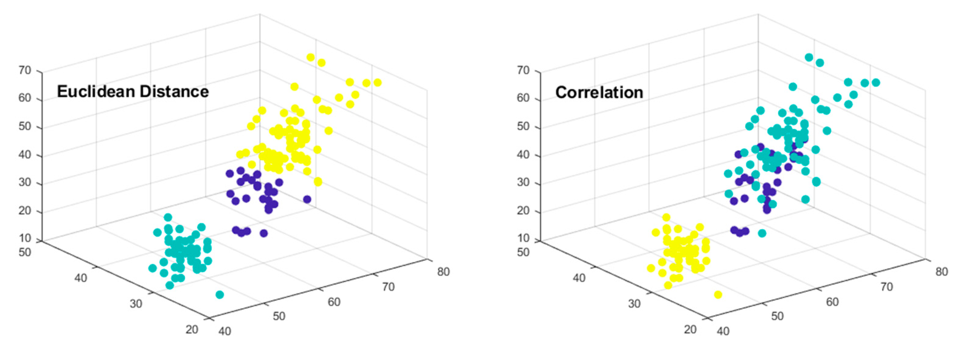
The K-means clustering algorithm uses the Euclidean distance to measure the distances between objects [20]. Other metrics can also be used, such as the Manhattan distance and Pearson correlation measure. The Euclidean distance is the most common use of distance; it computes the root of the square differences between the coordinates of a pair of objects.

The K-means clustering algorithm is a general clustering algorithm to cluster $N$ objects into $m$ groups of the number $m$. The method minimizes the total squared Euclidean distance $D$ of the form via the following equation:

$$D=\sqrt{{\displaystyle \sum _{k=1}^m{(x_{ik}-x_{jk})}^2}}$$

(7)

The K-means algorithm is performed in the following steps (Algorithm 1):

Algorithm 1. K-means clustering algorithm

Step 1. $\mathrm{Initialize} \mathrm{the} \mathrm{cluster} \mathrm{centers} c_j$ ($j$: the number of clusters needed to solve the task).   Set the initial cluster centers to the first $m$ training data or the $m$ randomly chosen training data.   Step 2. Group all the patterns with the closet cluster center.   $\mathrm{For} \mathrm{each} \mathrm{pattern} x_i$$, \mathrm{assign} x_i$$\mathrm{to} \mathrm{group} j^{*}$$, \mathrm{where} ‖x_i-c_{j^{*}}‖=\underset{j}{\min }‖x_i-c_j‖$.   Step 3. Compute the sample mean for the function center:             $c_j=\frac{1}{m_j}{\displaystyle \sum _{x_i\in group\hspace{0.17em}j}{x}_i}$   $\mathrm{for} \mathrm{each} \mathrm{group} c_j$$, \mathrm{where} m_j$ is the number of patterns in group $j$.   Step 4. Repeat by going to step 2, until there is no change in the cluster assignments.

The algorithm operates as follows. Initially, the $m$ centers are set to certain initial data points. If the training data was not ordered in any way, the first training data is typically chosen as the initial set of centers. Otherwise, the $m$ data points would be randomly selected. In step 2, each of the training patterns is assigned to the nearest center. In step 3, the centers are adjusted by computing the average in each cluster group. Steps 2 and 3 would be repeated until each training pattern remains in its group, i.e., no reassignment of any pattern to a different group than its previous one occurs.

As a result of the operation of the algorithm, the final cluster centers $c_j$ are determined, subject to the condition that the sum of the squared distances between all the points belonging to group $j$ and the cluster center must be minimal.

The popularity, high efficiency, and simplicity of the procedure can be considered as the advantages of the K-means algorithm. But in the case when the placement of objects is heterogeneous, the algorithm may not achieve good results. Then, it must change the parameters (the number of cluster centers or coordinates of the centers) and try to repeat the operation of the algorithm. The disadvantage is that the algorithm is not universal.

3.2. Illustrative Example

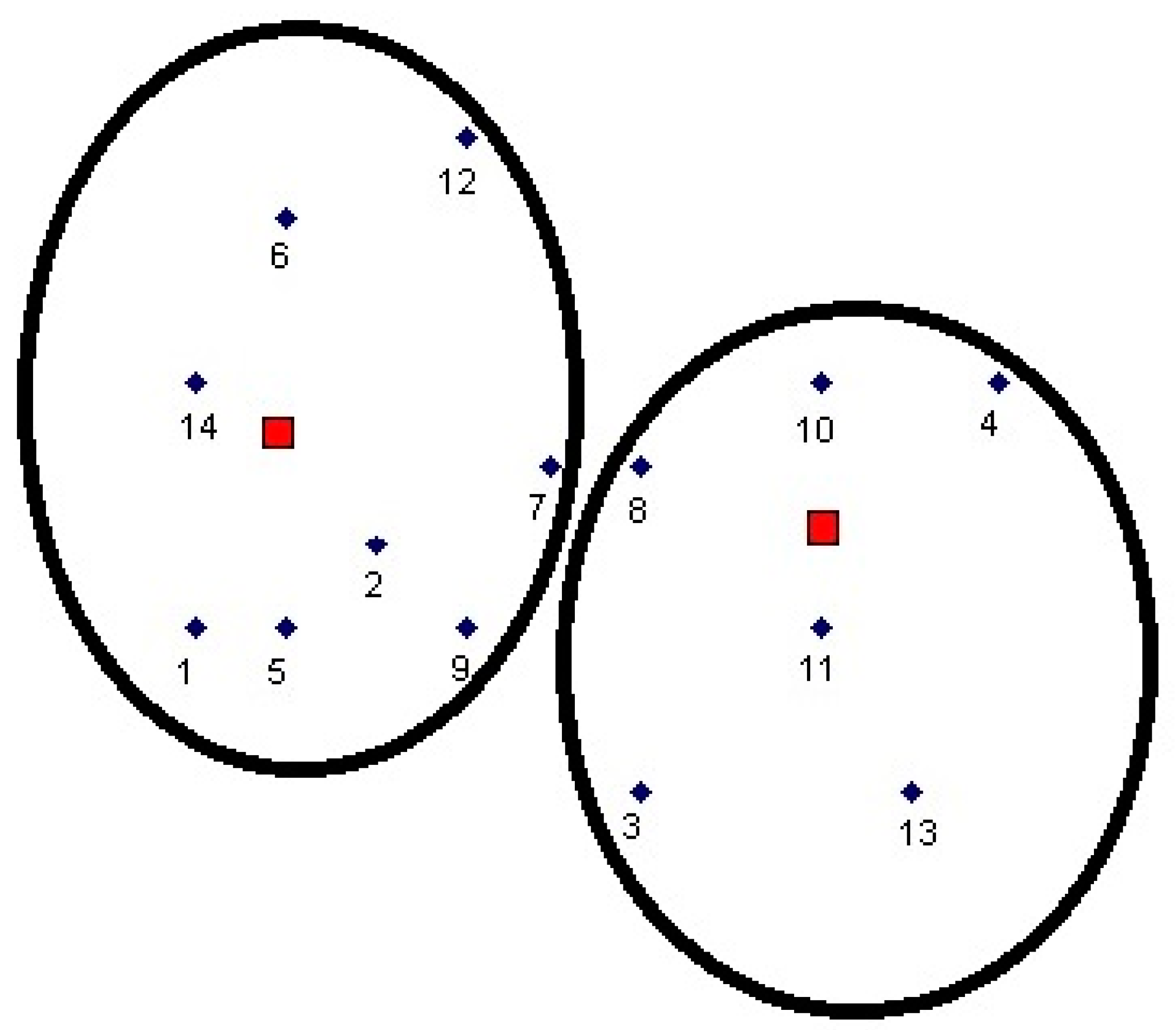
To test the potential of Cassini ovals for clustering purposes, a sample of artificial data with 14 points was proposed [22]. This dataset was used to illustrate the potential of utilizing clustering for working with Cassini ovals. The coordinates of the points are provided in

Table 1. The coordinates of the experimental data points.

	1	2	3	4	5	6	7	8	9	10	11	12	13	14
$x1$	1	3	6	10	2	2	5	6	4	8	8	4	9	1
$x2$	3	4	1	6	3	8	5	5	3	6	3	9	1	6

.

With the help of the K-means clustering algorithm, the following two clusters and their centers were obtained (Figure 2). Final cluster centres are marked as red rectangles.

If two clusters are selected, then the first cluster contains 8 data points (1, 2, 5, 6, 7, 9, 12, and 14) and the second cluster contains 6 data points (3, 4, 8, 10, 11, and 13). Clustering required three iterations of algorithm execution for two clusters. The final cluster centers are in coordinates (3, 5) and (8, 4).

For example, if three clusters are selected, then the first cluster contains 6 data points (1, 2, 5, 6, 12, and 14), the second cluster contains 6 data points (3, 7, 8, 9, 11, and 13), the third cluster contains 2 data points (4 and 10). Clustering required three iterations of algorithm execution for three clusters. The final cluster centers are in coordinates (2, 6), (9, 6), and (6, 3).

Cluster validity is a technique used to identify a group of clusters that most accurately represents natural divisions (the number of clusters) without relying on any class information. There are three primary criteria for assessing cluster validity: external criteria, internal criteria, and relative criteria [20]. In this instance, only the external cluster validity index was utilized to demonstrate the possibilities of cluster validity.

Given a dataset $X$ and a clustering structure $C$ derived from the application of a specific clustering algorithm on $X$, external criteria are used to compare the obtained clustering structure $C$ to a prespecified structure. This prespecified structure reflects prior information on the clustering structure of $X$.

For the external criteria, the comparison of the resulting clustering structure $C$ to an independent partition of the data $P$ is essential, as it was constructed based on intuition about the clustering structure of the dataset. Some commonly used external indices for assessing the correspondence between $C$ and $P$ are as follows: the Rand index, Jaccard coefficient, and the Fowlkes and Mallows index [20]. The Rand index measures the accuracy of determining whether a link belongs within a cluster or not.

All formulas are available in [20]. Our sole focus was on the computing values of the Rand index for the data in Table 1. In the case of two clusters, the Rand index is 1; in the case of three clusters, it is 0.72. The range for the first three indices is [0, 1]. High values of these indices indicate great similarity between $C$ and $P$.

We demonstrated the performance of the K-means clustering algorithm for the machine learning repository IRIS dataset with different distance metrics (Figure 3).

3.3. Clustering for Cassini Ovals

We then applied clustering to the Cassini ovals. We initially assumed that all the data points belonged to the same cluster.

For different values of $a$ and $b$, the following four cases are possible:

• case $b\ge 2a$

If $a=5$ and $b=10$, all data points lie inside the oval. One cluster is obtained (Figure 4).

b.

case $a<b<2a$

If $a=5$ and $b=9$, all points are inside the oval. One cluster is obtained (Figure 5).

c.

case $a=b$

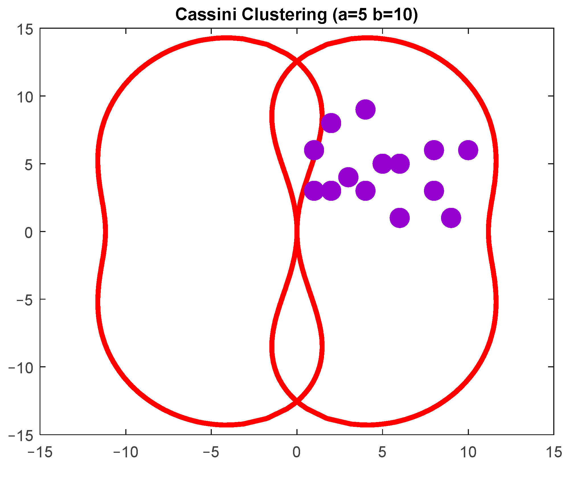
If $a=b$, seven data points are in the oval (Figure 6).

d.

case $a>b$

If $a=15,\hspace{0.17em}b=14$ and $a=16,\hspace{0.17em}b=15$, three data points are inside the oval. If $a=17,\hspace{0.17em}b=16$, four data points are inside the oval. The value of $b$ is $a-1$. The data points do not appear inside the oval at the lowest values of $b$ (Figure 7).

We concluded that in the 2-dimensional space, Cassini ovals can be used for clustering purposes.

4. Cassini Ovals in Radiolocation

In radiolocation, the target detection area is a curve bound by a Cassini oval if the position of the transmission source is taken as one of its focuses, and the position of the receiver is taken as the other focus. Similarly, in astronomy, when observing asteroids shining with reflected light from the Sun, the conditions for their detection at a certain telescope sensitivity are described by the Cassini oval formula. In this case, the detectability limit would be the surface formed by the rotation of the oval around the axis connecting the Sun and the observer.

“A bistatic radar is a radar that uses two antennas at separate locations, one for transmission and one for reception” [18].

In the Cartesian coordinate system $(x,y)$, there is a transmitter $F_1$ and a receiver $F_2$ on the axis $x$ symmetrically to zero (Figure 8). Let us find the reflector locus $M$, for which its observability from the receiver $F_2$ is constant. This is the set of points that $1/R_1^2{R}_2^2$ or which is equal to [17]:

$$R_1{R}_2=const$$

(8)

We set $F_{1}0=0F_2=c$ and expressed $R_1$ and $R_2$ in terms of $c$, $x$ and $y$. From Figure 8, the following can be observed:

$$R_1^2=y^2+{(x+c)}^2\hspace{0.17em}and\hspace{0.17em}{R}_2^2=y^2+{(x-c)}^2$$

(9)

Then, the following is true:

$$R_1^2{R}_2^2=a^4=[y^2+{(x+c)}^2][y^2+{(x-c)}^2]$$

(10)

After the transformations, the following equation is obtained:

$${(x^2+y^2)}^2-2c^2(x^2-y^2)=a^4-c^4$$

(11)

Equation (11) defines the Cassini oval, that is, the geometric locus of the points $M$ for which the product of the distances $R_1$ and $R_2$ from the two foci $F_1$ and $F_2$ is constant.

In radiolocation, the Cassini ovals have the following meaning. The same power would be sampled in focus from a target located at any point on the oval (if the transmitter radiating the target is at the second focus). If the power is at the sensitivity limit, then this oval covers the radar coverage area [17].

The bistatic radar uses two locations that are separated by a considerable distance. The transmitter is placed in one location and the associated receiver is placed in another location. Target detection is as follows: the transmitter illuminates the target, and the receiver receives and processes the target echo (Figure 9).

The distance from the receiver to the transmitter is known as the baseline $L$.

In the following study, we examined the application of Cassini ovals in the operation of bistatic radars, i.e., the determination of the bistatic radar coverage area.

Coverage can be defined as the region in the bistatic plane where the target is visible to both the transmitter and the receiver [18].

There are two ways to determine the bistatic radar coverage area:

(1)

The detection constraint, which is determined using the maximum range oval of Cassini;

(2)

The line-of-sight (LOS) constraint, which is determined using the geometry between the transmitter, target, and receiver.

In the following, we used notations and formulas from [18].

For specific transmitting and receiving sites, which established $L$, and for a constant bistatic maximum range product $k$, ${(R_T{R}_R)}_{\max }=k$ is the expression for a bistatic maximum range for Cassini ovals.

This equation can be rewritten as follows:

$${(R_T{R}_R)}_{\max }^2=\frac{K}{{(S/N)}_{\min }},$$

(12)

where $K$ is the bistatic radar constant and provided in [18]

$$K=\frac{P_T{G}_T{G}_R{\lambda }^2{\sigma }_B{F}_T^2{F}_R^2}{{(4\pi )}^{3}k{T}_s{B}_n{L}_T{L}_R}.$$

${(S/N)}_{\min }$ is signal-to-noise power ratio.

The characteristic values of the coefficient $K$ parameters were used from [18].

The ratio $S/N$ can be represented as Cassini ovals using the following:

$$(S/N)=\frac{K}{{(r^2+L^2/4)}^2-r^2{L}^2{\cos }^2(\theta )}.$$

(13)

For the detection constraint, when the Cassini oval encapsulates both the transmitter and the receiver, the coverage area can be approximated via [17,18]:

$$S\approx \pi k\left\{1-\left(\frac{1}{64}\right)\left(\frac{L^4}{k^2}\right)-\left(\frac{3}{\mathrm{16,384}}\right)\left(\frac{L^8}{k^4}\right)\right\}$$

(14)

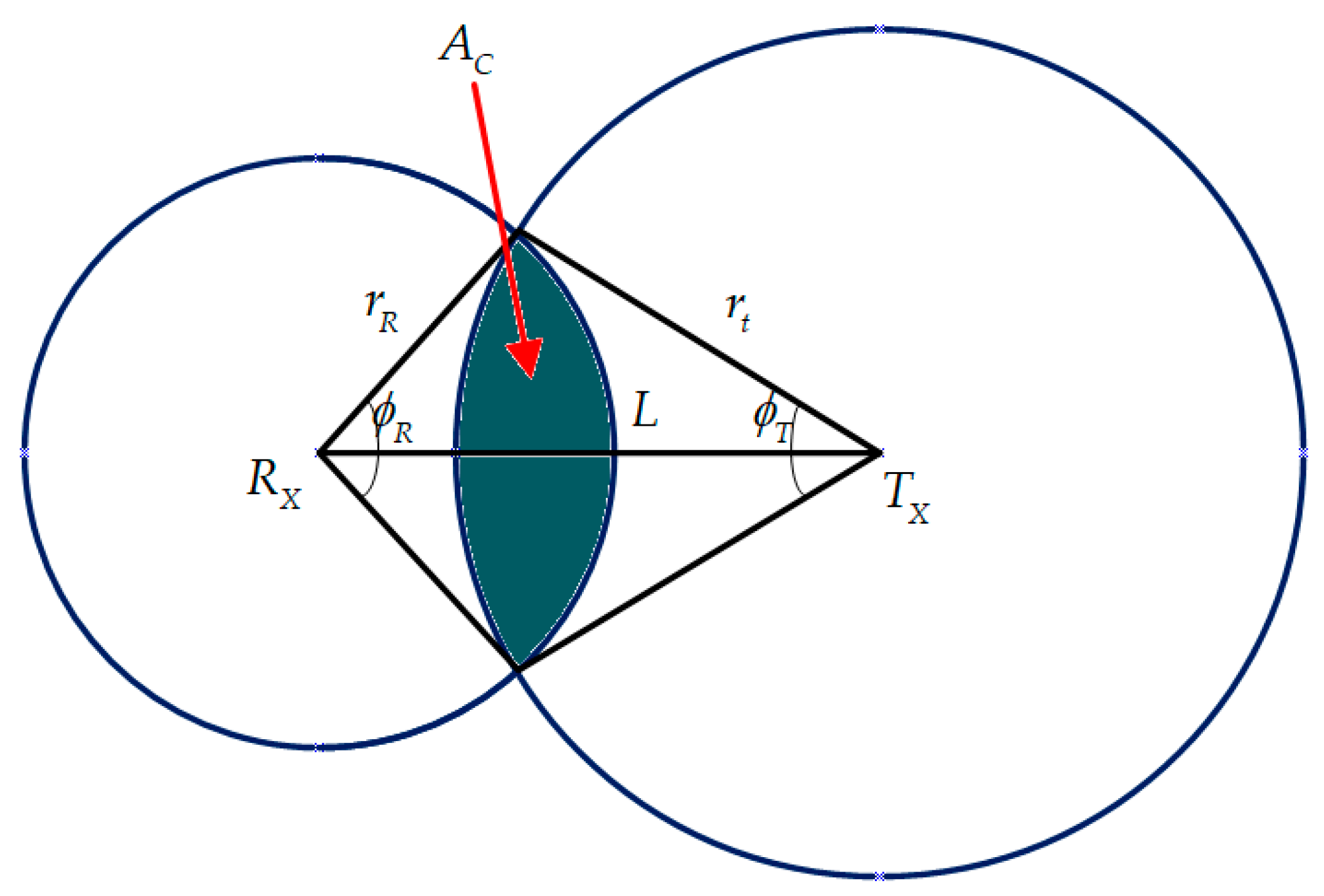
The LOS coverage is discussed below. The coverage area $A_C$ is defined by the total area covered by both the transmitter and receiver coverage circles, as shown in Figure 10 [18].

The radius of these coverage circles is provided in the following:

$$r_T=130(\sqrt{h_t}+\sqrt{h_T}),$$

(15)

$$r_R=130(\sqrt{h_t}+\sqrt{h_R}),$$

(16)

where

• $h_t$ = target altitude (km),
• $h_T$ = transmitter antenna altitude (km),
• $h_R$ = receiver antenna altitude (km).

The intersection of the two circles determines the common coverage area (for $L+r_T>r_R>L-r_T\hspace{0.17em}or\hspace{0.17em}L+r_R>r_T>L-r_R$) is the following:

$$A_C=\frac{1}{2}[r_R^2({\varphi }_R-\sin ({\varphi }_R))+r_T^2({\varphi }_T-\sin ({\varphi }_T))],$$

(17)

where

$${\varphi }_T=2\hspace{0.17em}{\cos }^{-1}\left(\frac{r_T^2-r_R^2+L^2}{2r_{T}L}\right),$$

$${\varphi }_R=2\hspace{0.17em}{\cos }^{-1}\left(\frac{r_R^2-r_T^2+L^2}{2r_{R}L}\right).$$

This results in the following equations:

$$A_C=0\hspace{0.17em}\hspace{0.17em}(r_T+r_R\le L).$$

(18)

$$A_C=\pi r_R^2\hspace{0.17em}\hspace{0.17em}(r_T\ge L+r_R).$$

(19)

$$A_C=\pi r_T^2\hspace{0.17em}\hspace{0.17em}(r_R\ge L+r_T).$$

(20)

As an example, let us determine the LOS coverage area for a remotely piloted aircraft (RPA) to be able to control the airspace. A RPA is an aircraft where the flying pilot is not onboard the aircraft. Current applications of small RPAs have antecedents from the early 1990s. Then, they were popularly called unmanned aerial vehicles, drones, and other names. The maximum altitude for drones in the European Union is 120 m above ground level.

Suppose that the transmitter and receiver is ground-based ($h_T=h_R=0$) and the maximum target altitude is $h_t=120\hspace{0.17em}\mathrm{m}=0.12 \hspace{0.17em}\mathrm{km}$. Using Equations (15) and (16), we can determine the values of $r_T$ and $r_R$. Substituting them into Equation (17), we can then obtain the area size of coverage. Starting with $L=10\hspace{0.17em}\mathrm{km}$ and a step of 10 km, we obtain the following results (

Table 2. The dependence of the coverage area on the baseline $L$ value for $h_t=0.12 \hspace{0.17em}\mathrm{km}$.

$L\hspace{0.17em}\hspace{0.17em}(\mathrm{km})$	10	20	30	40	50	60	70	80
$A_C\hspace{0.17em}\hspace{0.17em}({\mathrm{km}}^2)$	5470	4580	3720	2890	2110	1400	780	280

and Figure 11).

Similarly, it is possible to calculate the dependency, for example, for $h_t=0.5 \hspace{0.17em}\mathrm{km}$ (Figure 11).

After $L=80\hspace{0.17em}\mathrm{km}$ at this target altitude, the LOS coverage value $A_C$ becomes equal to 0.

We then increased the target height limit to 500 m. This allowed us to control not only drone flights, but also hot air balloons and low-flying helicopters. The results are shown in Figure 11. Moreover, in this case, after 180 km, the LOS coverage value $A_C=0$.

It could be concluded that in cases when the transmitter and receiver are closer to each other, the adequate LOS coverage is higher.

5. Discussion

Cassini ovals are used in astronomy, radiolocation, and various scientific applications, such as physics, biosciences, and acoustics. The unique properties of ovals mean they are an interesting tool in various fields for military and commercial purposes.

In this article, two completely different possibilities of using Cassini ovals were considered in radiolocation and clustering.

A study was conducted on determining the LOS coverage for low-flying targets when the transmitter and receiver are ground-based. Two fixed limits of target heights were chosen, and the coverage was determined for the specific parameters of the bistatic radar constant. By changing these parameters, the coverage area was different.

Terrain degrades bistatic coverage. For ground-based bistatic transmitters and receivers, degradation can be significant. For this reason, some air defense bistatic radar concepts use an airborne transmitter.

In the future, it is planned to focus on the research of detection-constrained coverage. This coverage is determined using the area within a maximum range of Cassini ovals, which is established using the bistatic maximum range product $k$.

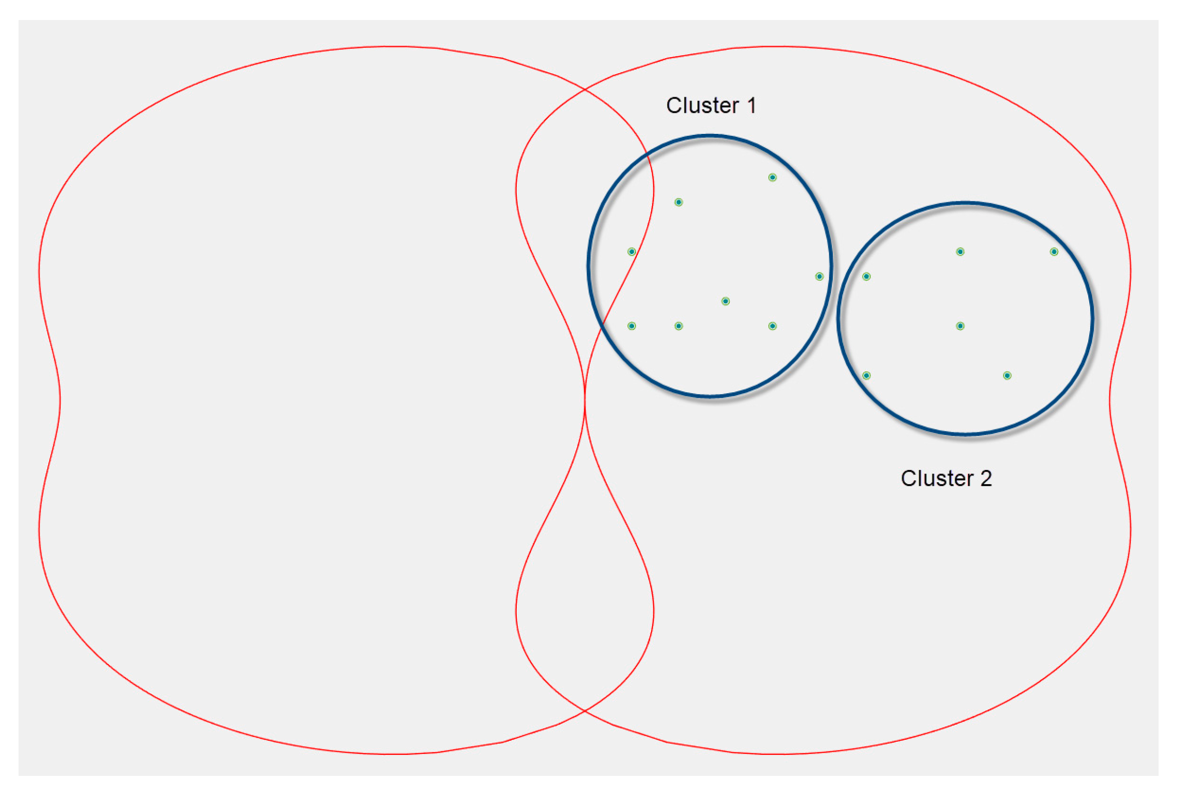
In the third section, we assumed that all the data points (objects) were in one cluster. Of course, this is a trivial case because the number and structure of the objects could be different. If, for example, the radar detects balloons and drones, then two clusters would be obtained in the clustering result, one of which would contain the projections of the balloons and the other one would have the projections of drone coordinates (Figure 12).

In the introduction section, it was noted that no similar works on the application of clustering to Cassini ovals were found, so the research methodology is currently in the development stage. A further work methodology is described using Algorithm 2.

Algorithm 2. Clustering in Cassini ovals

Step 1. Initialize the values of $a$ and $b$ for the Cassini ovals;   Step 2. Determine the size and shape of the Cassini ovals;   Step 3. Select the dataset;   Step 4. Specify the number of clusters;   Step 5. Apply the K-means algorithm (Algorithm 1);   Step 6. Validate clustering (if necessary);   Step 7. Reconcile the coordinates of the Cassini oval with the coordinates of the data to be clustered;   Step 8. Repeat by going to step 4 until acceptable clustering results are obtained.

The biggest problem now is to reconcile the coordinates of the Cassini oval with the coordinates of the clustered data.

The study is currently in its early stages and the authors have not rejected the proposed hypothesis of the use of clustering for Cassini ovals and will continue their research.