Abstract
Fault data under real operating conditions are often difficult to collect, making the number of trained fault data small and out of proportion to normal data. Thus, fault diagnosis symmetry (balance) is compromised. This will result in less effective fault diagnosis methods for cases with a small number of data and data imbalances (S&I). We present an innovative solution to overcome this problem, which is composed of two components: data augmentation and fault diagnosis. In the data augmentation section, the S&I dataset is supplemented with a deep convolutional generative adversarial network based on a gradient penalty and Wasserstein distance (WDCGAN-GP), which solve the problems of the generative adversarial network (GAN) being prone to model collapse and the gradient vanishing during the training time. The addition of self-attention allows for a better identification and generation of sample features. Finally, the addition of spectral normalization can stabilize the training of the model. In the fault diagnosis section, fault diagnosis is performed through a convolutional neural network with coordinate attention (CNN-CA). Our experiments conducted on two bearing fault datasets for comparison demonstrate that the proposed method surpasses other comparative approaches in terms of the quality of data augmentation and the accuracy of fault diagnosis. It effectively addresses S&I fault diagnosis challenges.
1. Introduction
Bearings constitute a pivotal element in the mechanics of machinery with rotating elements [1]. The diagnosis of faults in bearings is of significant importance. However, in real working conditions, mechanical equipment tends to operate normally most of the time and rarely experiences failures. As a result, collected data mostly pertain to normal operating conditions, with only a small amount of data related to faults [2,3]. S&I samples, compared to normal samples, have small sample sizes and imbalanced proportions [4]. Compared with the traditional method of fault diagnosis for balanced samples, the method of fault diagnosis in the case of S&I samples is of great significance for the application of intelligent fault diagnoses [5]. The asymmetry (imbalance) between the sample sizes of different data categories reflects the real scenario; thus, we need to make the sample sizes between data categories symmetrical.
In the field of deep-learning-based mechanical fault diagnosis, there are three methods based on different approaches to address the problem of S&I data. They are data-augmentation-based methods, transfer-learning-based methods, and model-based methods [6]. Among them, data augmentation is an effective method to solve the problem of S&I data. Data augmentation is the process of generating new data samples based on the distribution of the original data [7]. This method solves the problem of missing data; it can provide high-accuracy fault diagnoses without relying on the overly complex fault diagnosis model. Many scholars have been using data augmentation to generate more new samples to solve the S&I problem [8,9,10]. The initial stage of the augmentation of the dataset is based on two-dimensional images. For the data augmentation of one-dimensional vibration signals, routine data augmentation methods such as adding noise as well as slicing, scaling, and rotating the vibration signals for time-series can be used, in addition to deep learning models similar to those used for generating images [11].
GANs are used as a basic technique for generative modelling, which has the ability to generate new samples that are similar to the original samples. The GAN and its variants have received more and more attention in the field of fault diagnosis [12,13,14]. In order to solve the problem of the poor quality of one-dimensional data and limited learning datasets, Pajak et al. [15] performed data augmentation by slicing and randomly disrupting the original one-dimensional time domain signal. Yang et al. [16] addressed the issue of insufficient bearing data by first converting the original vibration signals into grayscale images. They then proposed a new method called CGAN-2-D-CNN, which combines conditional generative adversarial networks with 2-D convolutional neural networks to generate new samples. Li et al. [17] designed an innovative model based on assisted classifier generative adversarial networks (ACGANs) combined with Wasserstein distance as well as a gradient penalty. Their model could better address the problems of the low generation efficiency of generative adversarial networks, model collapse, and gradient vanishing. Additionally, they incorporated a gradient penalty to overcome associated issues. Furthermore, spectral normalization was introduced to ensure stable model training. These modifications were made to overcome the aforementioned challenges and improve the efficiency and stability of fault sample generation in GANs. Gu et al. [18] proposed a cosine similarity-based self-attention Wasserstein gradient penalty GAN to address the issue of imbalanced faulty data. It converts vibration signals into frequency domain samples, which can provide a clearer spectrum, and generates new samples. Li et al. [19] proposed a conditional Wasserstein GAN based on a gradient penalty as well as a gated recurrent unit neural-network-based fault diagnosis framework for the problem of imbalanced data in bearing fault diagnoses.
Our review of the literature shows how scholars use GANs and variants of GANs to solve problems when there are not enough samples for fault diagnosis. But GANs have some problems, as shown by the current research. Firstly, GANs are prone to instability during the training process. GANs simultaneously have poor generation quality and limited diversity. Lastly, GAN training typically demands a substantial amount of original data and can be time-consuming due to the complex nature of the model. Many scholars have addressed these issues by modifying the GAN loss function and adding different types of modules to the GAN network to address imbalances in the ratio between fault data and normal data as well as the small amount of fault data for bearing fault diagnoses. Meanwhile, others aim to alleviate the problems of model collapse and gradient vanishing that occur in the training process of GANs. In our method, the vibration signals of bearings are firstly converted into time frequency (TF) images through data preprocessing, after which the WDCGAN-GP is trained to generate new samples to solve the S&I problem. The expanded new dataset is inputted into the CNN-CA to complete the fault diagnosis. The main contributions of this article can be summarized as follows:
- This article proposes a novel fault diagnosis method using a generative adversarial network (WDCGAN-GP) combined with CNN-CA, which firstly trains a small number of samples and generates high-quality samples, then adds the generated samples into the initial S&I dataset, which better solves the problem of the poor accuracy of fault diagnoses in the case of S&I data.
- The method we propose introduces Wasserstein distance and a gradient penalty based on a deep convolutional generative adversarial network (DCGAN) with a self-attention mechanism added to the generative model. Additionally, spectral normalization is used to stabilize the model training. The WDCGAN-GP solves the problems of GAN model collapse and gradient vanishing. At the same time, it also enhances the quality of the model’s generated samples. The addition of the coordinate attention mechanism also makes the CNN better at performing fault diagnoses.
- The proposed method’s reliability was validated using two distinct bearing datasets, with the quality of the generated samples evaluated using Fréchet inception distance (FID) and structural similarity (SSIM) metrics. The results demonstrated that, compared to other methods, the proposed approach effectively addressed the problem diagnosing faults when dealing with S&I data.
The rest of the content of this article is structured as follows. In Section 2, the relevant theoretical background is summarized. Section 3 expounds on the detailed information of our proposed fault diagnosis method. Section 4 presents the experimental results and a discussion of the proposed method compared to other methods with different datasets. Section 5 draws conclusions on the reliability of our method and identifies some of its limitations.
2. Theoretical Background
2.1. Continuous Wavelet Transform
TF images can better present information about vibration signals in the time domain as well as in the frequency domain compared to vibration signals and can help in the subsequent diagnosis of faults to obtain better identification results [20]. Continuous wavelet transform (CWT) can decompose or represent vibration signals based on different basis functions. The resulting TF images contain detailed information about the time and frequency domains of the vibration signal. Compared with the short-time Fourier transform (STFT), CWT does not need to select the window size, avoiding situations in which the frequency analysis of the signal is not precise enough due to the small selection of the window of the STFT and the low resolution in the time domain due to the large selection of the STFT. Thus, the CWT has the same temporal resolution as the original data in each frequency band [21]. Therefore, the CWT is the best TF transform tool to analyze non-stationary signals [22]. It is specifically defined in the following Equation (1):
In the given equation, the input vibration signal is represented by , the wavelet basis function (WBF) is denoted as , the conjugate complex of is represented as , the scaling factor a determines the expansion and contraction of the WBF, and the translation factor determines the position of the WBF. The WBF has different effects on the processing of vibration signals. The Morlet basis function has a good level of smoothness. In comparison with the DB basis function, the Morlet WBF can better reflect the high and low amounts of energy concentrated in the vibration signal. It aims to extract fault characteristics from bearing vibration signals in a more reasonable and effective manner [23]. Therefore, we chose the Morlet function as the WBF for the CWT.
2.2. Generating Adversarial Networks
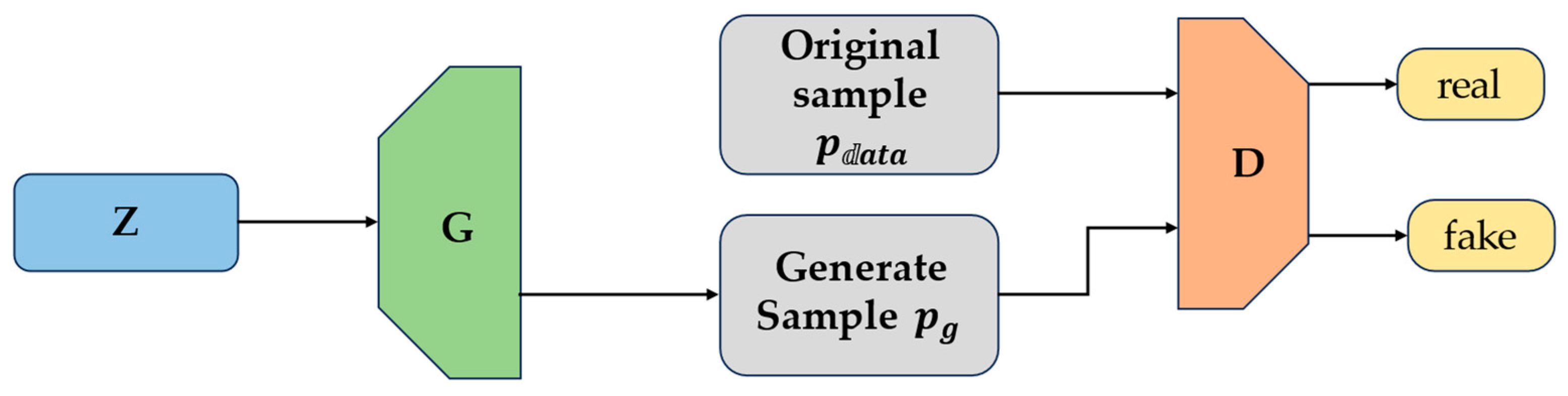
GANs, proposed by Goodfellow et al. [24] in 2014, are unsupervised generative models that offer solutions for data augmentation and data imbalances. The underlying principle of the model is rooted in the concept of zero-sum game theory. The entire network primarily comprises two network modules: the generator (G) and the discriminator (D). The G is tasked with acquiring knowledge about the feature distribution within the known data space and generating new samples based on the learned feature distributions. On the other hand, the D functions as a binary classification network, examining the disparities between the real samples and the generated samples. The model engages in a continuous adversarial process, with the G and D constantly opposing each other. Through iterative optimization using the back-propagation of the loss function, the two neural network modules strive to achieve the Nash equilibrium, at which point neither module can improve its performance without affecting the other. The GAN model framework is shown in Figure 1.
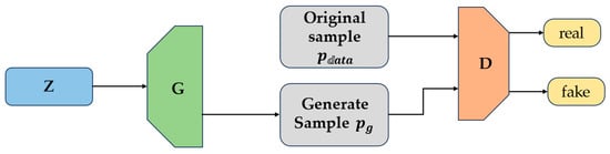
Figure 1.
GAN framework diagram.
The key core of the GAN lies in the loss function construction of the G and D. The two network models are trained by making the loss function converge to the minimum and maximum. The loss function of GAN is defined in the following Equation (2):
and denote the probability distributions of the actual sample and random noise, respectively. The discriminator’s output represents the likelihood that the outputs are real samples. refers to the generated sample data produced by the G using random noise. If < 0.5, it is classified as a real sample; otherwise, it is considered a generated sample. In contrast to other neural networks that aim to minimize the loss function, the G is continuously optimized to approach the minimum loss function, whereas the D is continuously optimized to approach the maximum loss function.
The DCGAN [25] uses full convolutional layers instead of the linear layers of the original GAN, which enables it to better learn the distribution of data features through the feature extraction capability of the convolutional module. The differences between the DCGAN and the GAN are as follows:
- The G eliminates all pooling layers in the network using transposed convolutions for upsampling, while the D uses convolutions with strides instead of pooling layers.
- The removal of the fully connected layers of the network in order to transform it into a fully convolutional network.
- The last layers of the G and D, which use tanh and sigmoid as activation functions, respectively.
- The D uses LeakyReLU as the activation function to prevent gradient sparsity.
2.3. Wasserstein Distance and Gradient Penalty
During training, GANs are susceptible to issues like model collapse and gradient vanishing. The original GAN is challenging to train and demands a significant amount of time and effort to fine-tune the network parameters of the G and D during the testing process [26]. To address the aforementioned challenges, Arjovsky et al. [27] introduced the Wasserstein GAN (WGAN). By replacing the original Jensen–Shannon divergence (JS divergence) and Kullback–Leibler divergence (KL divergence) with Wasserstein distance, the WGAN improves the measurement of differences between real and generated samples. This modification allows for more effective training and better captures the underlying data distribution. The emergence of the WGAN solves the problem of the model being difficult to train. Wasserstein distance is defined as shown in Equation (3) as follows:
and denote the data distributions of the generated and original samples, respectively. denotes that all data distributions belong to the joint distribution , and denotes the expected value of the distance between x and y. A gradient penalty (GP) can be introduced to improve the quality of the generated samples, while preventing problems such as model collapse and gradient vanishing.
The introduction of the GP can improve the quality of the generated samples on the basis of the WGAN. At the same time, it can prevent problems such as model collapse and gradient vanishing [28]. The GP can be expressed as shown in Equation (4) as follows:
represents the coefficient for the GP, denotes the L2 norm of the gradient, and represents a randomly sampled point from the sample space that includes both real and generated samples. represents inputting into the D and computing the corresponding gradient. denotes the expectation operation for the generated samples according to the probability distribution .
2.4. Spectral Normalization
For the purpose of solving the instability in network training, Miyato et al. [29] proposed a new weight matrix normalization method called spectral normalization (SN). The number of parameters in the network model grows exponentially with the number of network layers, leading to an increase in the probability of gradient explosion. The Lipschitz function continuity is controlled by limiting the number of spectral paradigms (L2 paradigms) of the weight matrix at each layer of the network. The formula for SN is shown in Equation (5) as follows:
When is used to normalise the weight matrix so as to obtain , i.e., the Lipschitz constraint is fulfilled, we can transform the training instability problem of the GAN into the task of obtaining the maximum singular value , which can be viewed as an application of the power iterative method [30]. The specific flow of the computation is as follows in Equations (6)–(8):
2.5. Self-Attention Mechanism
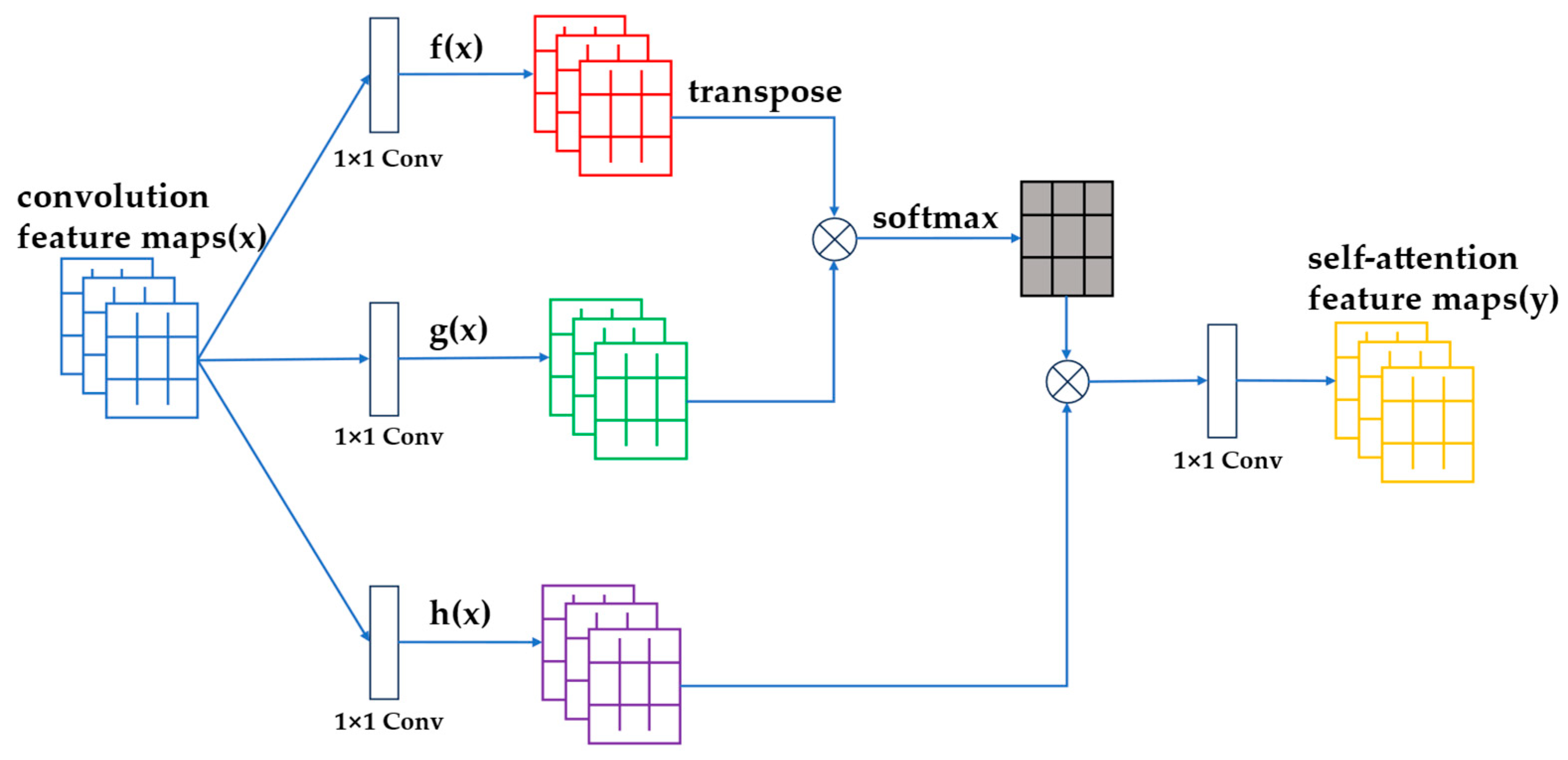
Due to not being able to learn deep features of TF images, the quality of generated data is often unsatisfactory in some models in the GAN. A self-attention mechanism (SA) added to the G and D can better extract different fault features in TF images and improve the generation quality of GANs [31]. An SA mechanism can effectively learn the global features in different samples instead of considering only local features and then accumulating them. In the SA mechanism, three 1 × 1 convolutional layers are utilized to produce three distinct sub-feature maps, denoted as f(x), g(x), and h(x), based on the input feature maps. Following this, the transposed convolution matrix of the sub-feature map f(x) is combined with g(x) to derive the respective attention weights. The transposition of the sub-feature map f(x) is multiplied by g(x) to obtain the corresponding attention weights. After processing these through the Softmax activation function, a new attention map is obtained. Finally, the matrix is multiplied with h(x) and a 1 × 1 convolutional block, yielding the final SA feature map. The detailed structure diagram is shown in Figure 2 as follows.
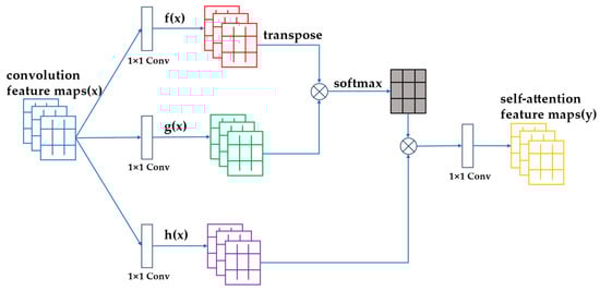
Figure 2.
Self-attention framework map.
The formula for the SA mechanism is shown in Equations (9) and (10) as follows:
where denotes the degree of attention paid by the SA module to the th position at the th region in the image, is the number of feature positions of the previous hidden layer feature, is the input feature map, is the final output feature map, and is the learnable parameter. The addition of the SA mechanism helps the G to better learn the data distribution in the original sample space, which can improve the quality of the generated samples. Adding an SA mechanism in the D enhances its discriminative ability. An excellent D can urge the G to improve the quality of the generated samples.
2.6. Coordinate Attention Mechanism
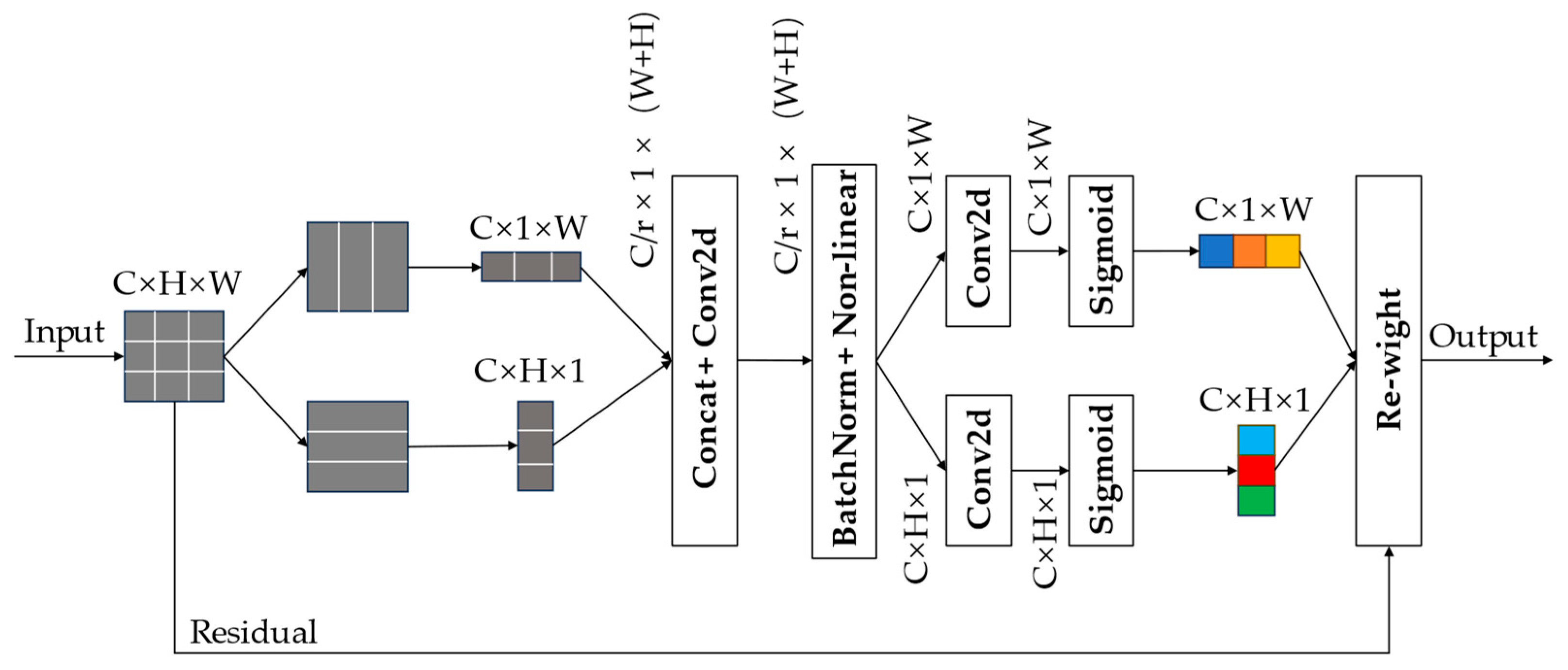
While the traditional squeeze and excitation (SE) mechanism can focus on different channels’ level of importance, the coordinate attention (CA) mechanism also encodes spatial information [32]. The CA module applies attention in both the horizontal and vertical directions simultaneously to the input tensor. Each element in the attention map captures relevant features from its rows and columns independently. This encoding process enables the CA to precisely determine the exact location of the extracted features, thereby enhancing the classification model’s ability to recognize these features effectively. A detailed structural diagram of the CA module is shown in Figure 3 as follows.
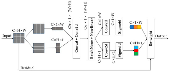
Figure 3.
Coordinate attention structure.
When the input is provided, the pooling kernel of the CA module with the dimensions (H, 1) or (1, W) encodes each channel along the horizontal and vertical CA axes. The output of channel at height can be calculated using Equation (11) as follows:
Similarly, the output for channel at width is shown in Equation (12) as follows:
Afterwards, the features of the above Equations (11) and (12) are mapped. Subsequently, the two are concatenated and finally passed to the common 1 × 1 convolutional transform function , from which Equation (13) can be obtained as follows:
where the notation [ , ] represents a series operation performed along the spatial dimension, and the symbol represents a nonlinear activation function. The intermediate feature mapping encodes spatial information in both the horizontal and vertical directions. The reduction rate r is chosen as 32 to reduce the computational overhead. Additionally, two separate 1 × 1 convolutional transforms, and , are applied to convert and into tensors with the same number of channels as , which can be obtained as follows in Equations (14) and (15), respectively:
where is the Sigmoid function, and and are expanded as the weights of the attention module. The overall CA module can be written as Equation (16) as follows:
2.7. Assessment Indicators
In this article, FID [33] and SSIM [34] are chosen as the metrics for evaluating the generated samples compared to the original TF image samples. SSIM is calculated by comparing the two images in terms of their luminance, contrast, and structure, which are weighted and expressed as a product. The value of SSIM is in the interval of [−1, 1]. The closer the value is to 1, the greater the similarity between the two images. When two identical images are assessed, the SSIM value is 1. The specific formula of SSIM is shown in Equation (17) as follows:
Here, , , , , and are the mean, variance, and covariance based on the real image and the generated image, which also represent the features of the real image and the generated image. In addition, , , and , where is the pixel value of the image. SSIM considers the similarity of the two images. Meanwhile, FID is evaluated in terms of the similarity between and diversity of the generated samples and the original samples: the smaller the value of FID is, the better the diversity and similarity of the image. The calculation formula is shown in Equation (18) as follows:
where and are the mean vectors of the original and generated data distributions, respectively, and are the covariance matrices of the original and generated data distributions, respectively, and denotes the trace of the computational matrix.
3. Proposed Method
3.1. Overall Framework
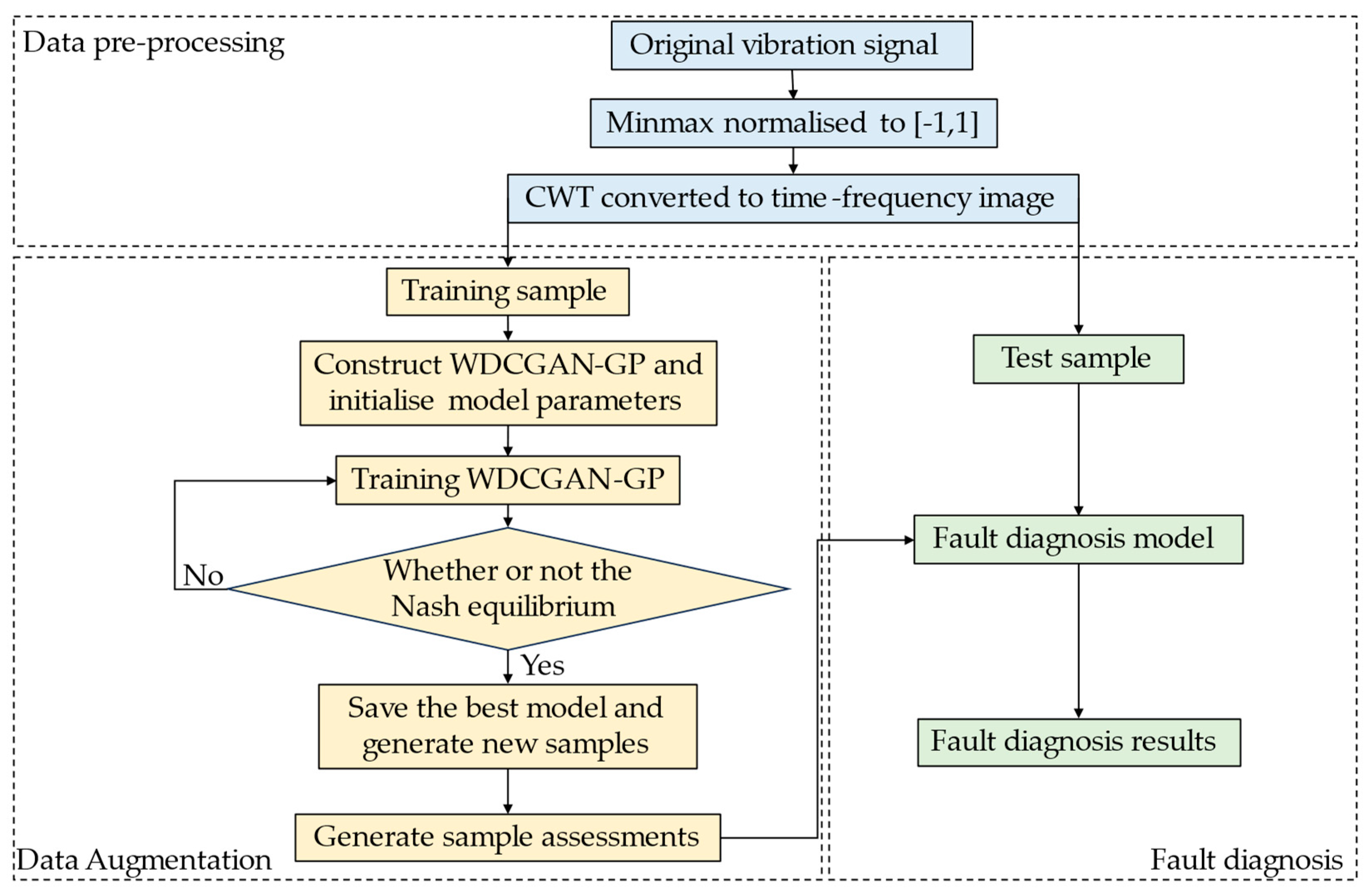
This article presents a novel fault diagnosis method in cases of S&I data. The proposed approach utilizes WDCGAN-GP for data augmentation. The enhanced sample data are subsequently employed for fault diagnoses using CNN-CA. A detailed structure diagram of overall process is shown in Figure 4.
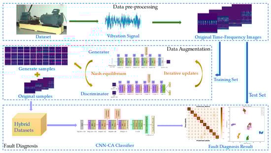
Figure 4.
Method process diagram.
Figure 4 contains three main parts: data preprocessing, data augmentation, and fault diagnosis. Firstly, in the data preprocessing part, the original vibration signals are min–max normalized. The distribution of the data is controlled to be between [−1, 1], which can better highlight the characteristics of the faulty data points [35]. The vibration signals are transformed into TF images with dimensions of 128 × 128 through CWT. The transformed TF images are divided into training samples and testing samples based on the quantity. The training samples are used as the training data for the generation model, while the testing samples are used for testing in the fault diagnosis part.
In the data generation part, the G and D of WDCGAN-GP are designed based on the network structure of all transposed convolutional and all convolutional layers. The G mainly consists of an all transposed convolutional layer and an SA module, whose input is a random noise vector and whose output is a generated image sample. The discriminator, on the other hand, has the original TF image samples and the generated samples as its input, and its output is the discriminator’s result based on the input images. The two networks reach the state of Nash equilibrium through mutual games and iterative updates. It is worth noting that, according to the principle of the GAN loss function, the essence of training in a GAN network is to seek the minimum and maximum values of G and D. G is updated to improve the quality of generation based on the identification results of D. D identifies the original samples and the samples generated by G in each round of training. Finally, G and D reach a dynamic equilibrium in the iterative updating of one another, i.e., neither network changes itself to obtain better results, and this state can be called the Nash equilibrium for the iterative training of the GAN. At the end of WDCGAN-GP generation, we also perform a generation quality assessment for the generated samples using SSIM as well as FID, with the aim of confirming that the generated samples have a high degree of similarity to the original samples.
In the fault diagnosis section, the original S&I dataset and the generated samples with the original S&I dataset form a new hybrid dataset to be inputted into the CNN or CNN-CA for fault diagnoses, respectively. The effectiveness of the method is determined based on a comparison of the accuracy of the different fault diagnoses. A detailed structure diagram of technology roadmap is shown in Figure 5.

Figure 5.
Technology roadmap.
3.2. Generator Architecture and Parameters
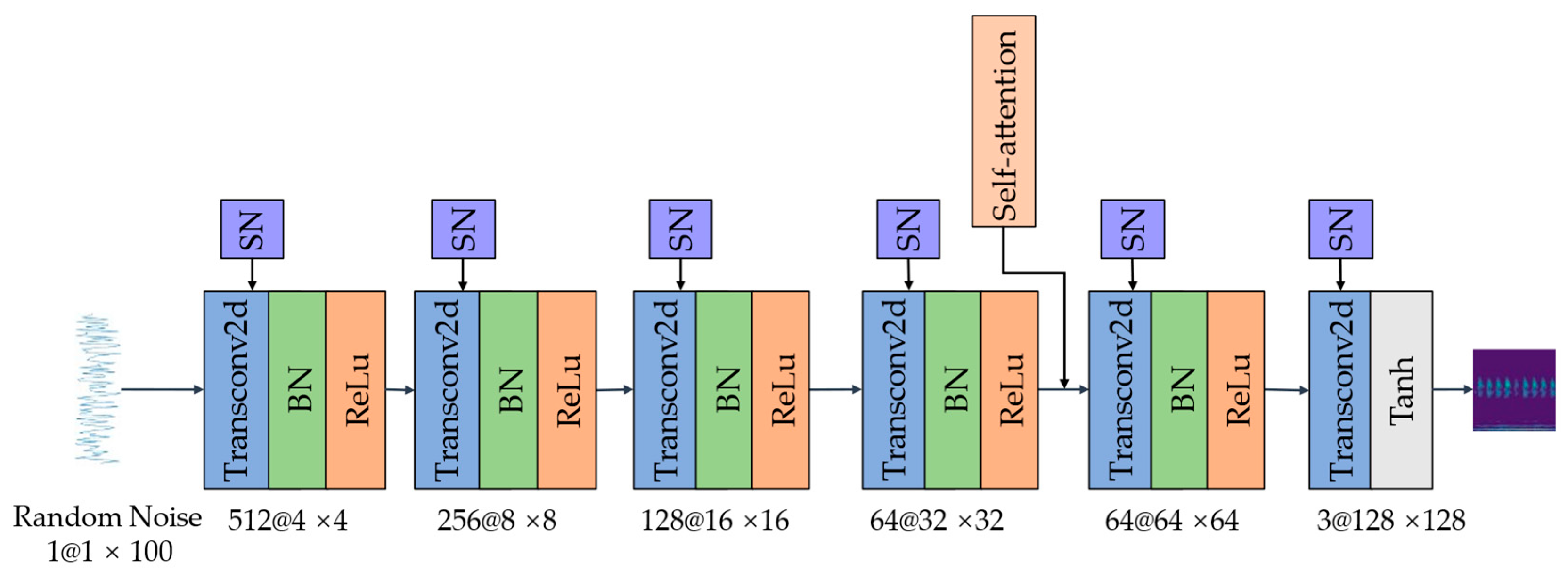
The input of the G is a 100-dimensional Gaussian random noise vector z, which is used to generate a 128 × 128 output image. The transpose convolution modules in the G utilize SN for weight normalization. The SA is introduced between the fourth and fifth layers of the model to improve the quality of generated images. Finally, the output is limited to the range of [−1, 1] using the Tanh activation function. Batch normalization (BN) is applied after each layer of the G network to accelerate training speed and prevent overfitting. A detailed diagram of the G’s structure and its parameters is shown in Figure 6.
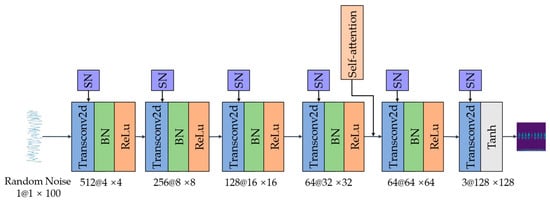
Figure 6.
Diagram of generator’s structure and parameters.
3.3. Discriminator Architecture and Parameters
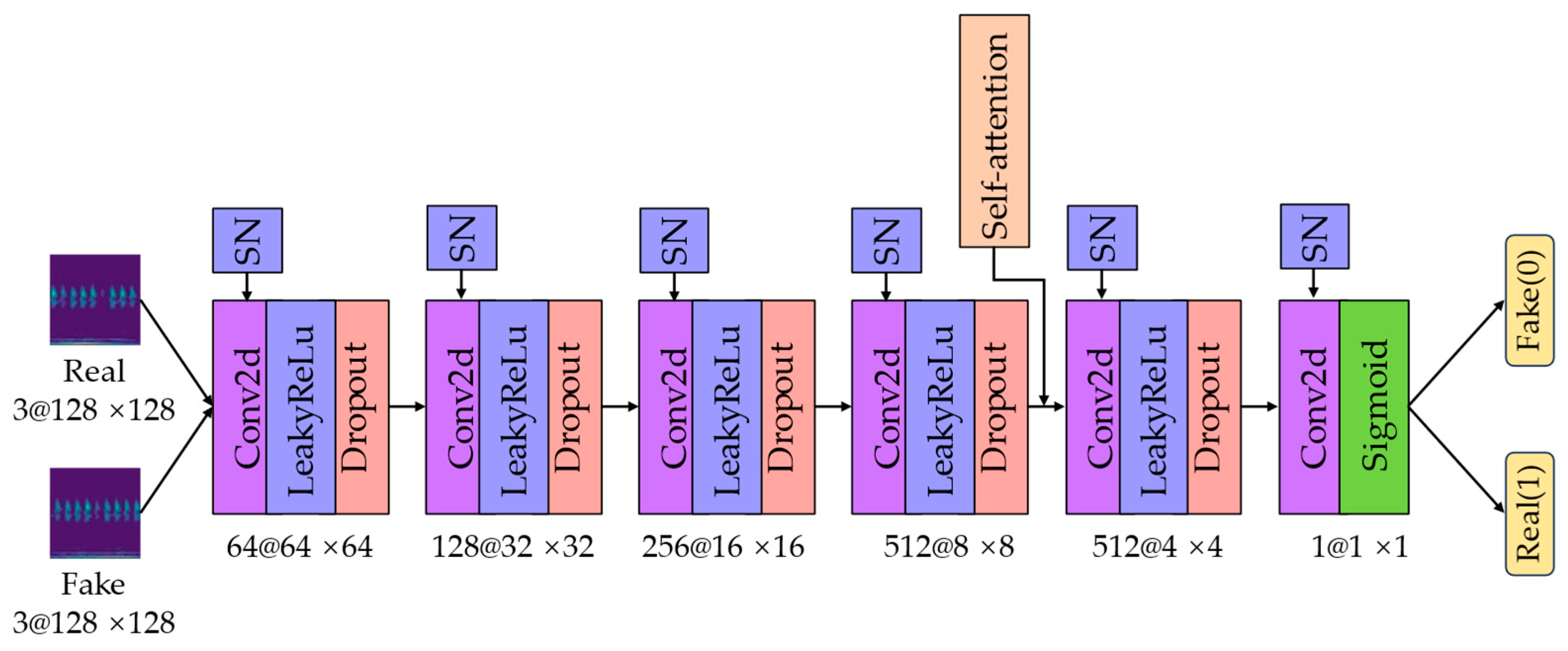
The inputs of the D are the original TF image samples and the generated TF image samples. The outputs of the D are obtained using the sigmoid activation function, which provides true or false discrimination results. This allows the D to determine whether the input samples are original or generated samples. The D contains modules consisting of 5 layers of convolution and LeakyReLU function, which enable the D to discriminate the types of samples more accurately. At the same time, dropout is added after the activation function to prevent the model from overfitting. SN is used in the network to perform the weight normalization operation for each convolution module. The SA is added between the fourth and fifth layers of the D to enhance its discriminative capability. A detailed diagram of the D’s structure and its parameters is shown in Figure 7.
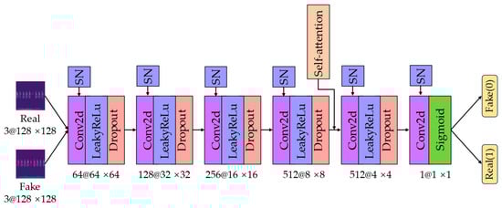
Figure 7.
Discriminator’s structure and parameters.
3.4. Loss Function and Generative Model Training
WDCGAN-GP is based on the DCGAN model, and SN, Wasserstein distance, and GP are introduced to improve the model training. The loss function of WDCGAN-GP is shown in Equation (19) as follows:
where and represent the predicted values from the original and generated data, is the GP coefficient, denotes the joint data distribution of the original and generated data, and denotes the data obtained by interpolation according to the original and generated data in the GP. In the generative model, the input consists of 2-D TF images. Afterwards, the G and D undergo adversarial training to enhance the generation quality of the G and improve the recognition ability of the discriminator. This iterative training process helps optimize both models to achieve better performance. The detailed parameters of WDCGAN-GP training are. as shown in Table 1.

Table 1.
WDCGAN-GP training parameters.
A detailed structural diagram of training flow of WDCGAN-GP is shown in Figure 8.
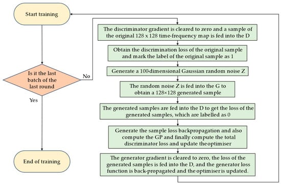
Figure 8.
WDCGAN-GP training flowchart.
3.5. Fault Diagnosis Model
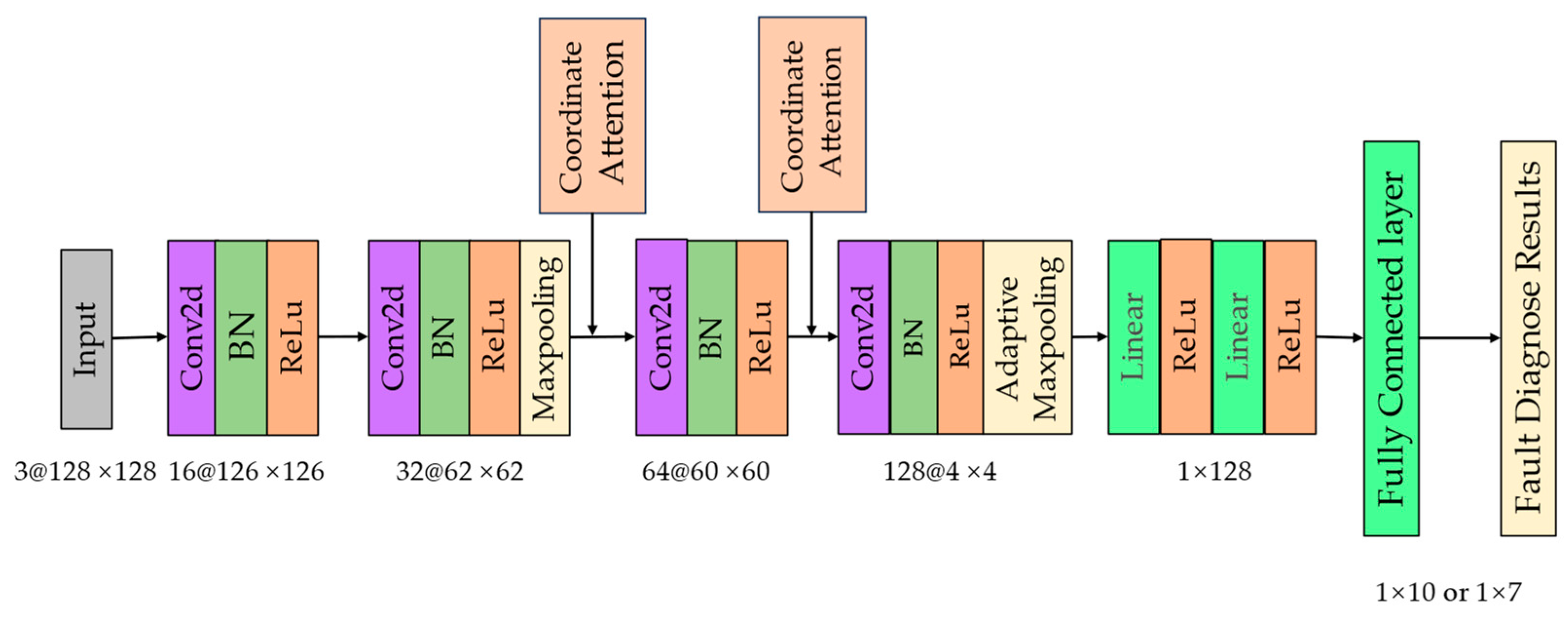
Our proposed method uses CNN-CA as a fault diagnosis model, in which the input is original S&I dataset or a mixed dataset consisting of the generated samples and the original S&I dataset. The CNN-CA contains a total of four convolutional layers, each of which containing a 3 × 3 convolutional module as well as the BN and ReLU activation functions. The model adds CA in the second layer and the third layer of the underlying CNN after the second and third layers. Finally, the classification is performed using the linear layer and Softmax activation function. The batch size is set to 32. Using Adam optimizer and a learning rate of 0.001, the epoch rounds are set to 30. The detailed structural diagram of CNN-CA and its parameters is shown in Figure 9.
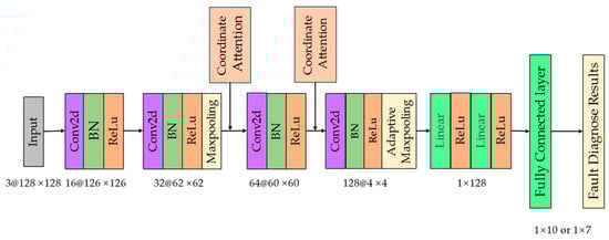
Figure 9.
CNN-CA structure and parameter diagram.
4. Experimental Research and Analysis
Our experimental study selected Case Western Reserve University (CWRU)’s bearing fault dataset and Xi’an Jiaotong University Spectra Quest (XJTU-SQ)’s bearing fault dataset as data sources for diagnoses of S&I bearing faults. The CWRU dataset is based on the data collected from bearings of different sizes with different faults, while the XJTU-SQ dataset is based on the fault data collected from bearings with different levels of damage to the inner and outer rings. The effectiveness of the proposed method is verified by experiments using the two different datasets. The computer system utilized is Windows 11, equipped with a 2.7 GHz Intel Core i7-12700H CPU. The GPU employed for accelerating the model training is an NVIDIA GeForce RTX3070Ti. Python 3.7.16 is used as the programming language, and Pytorch 1.13.1 is used as the deep learning framework.
4.1. Experiments on the CWRU
4.1.1. CWRU Bearing Dataset
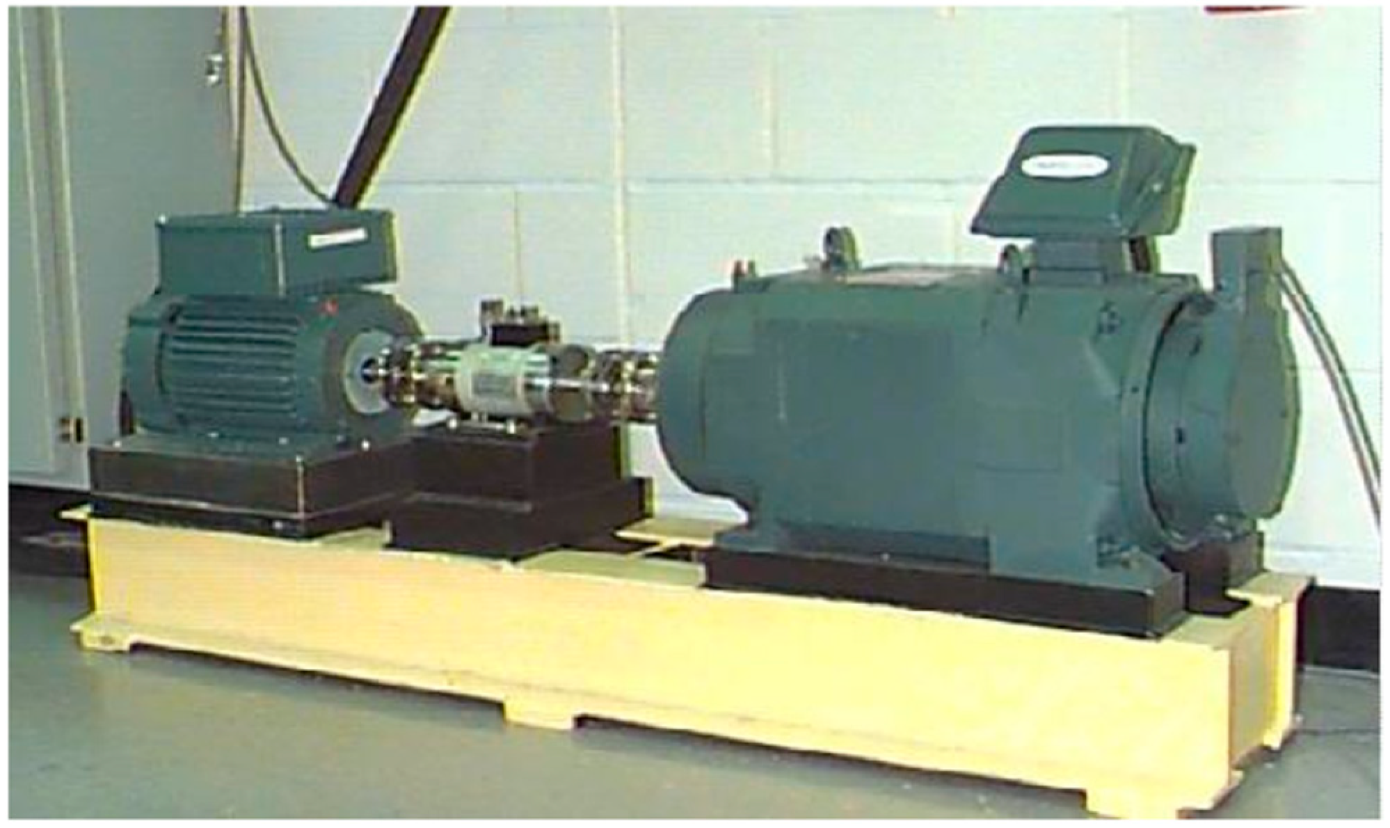
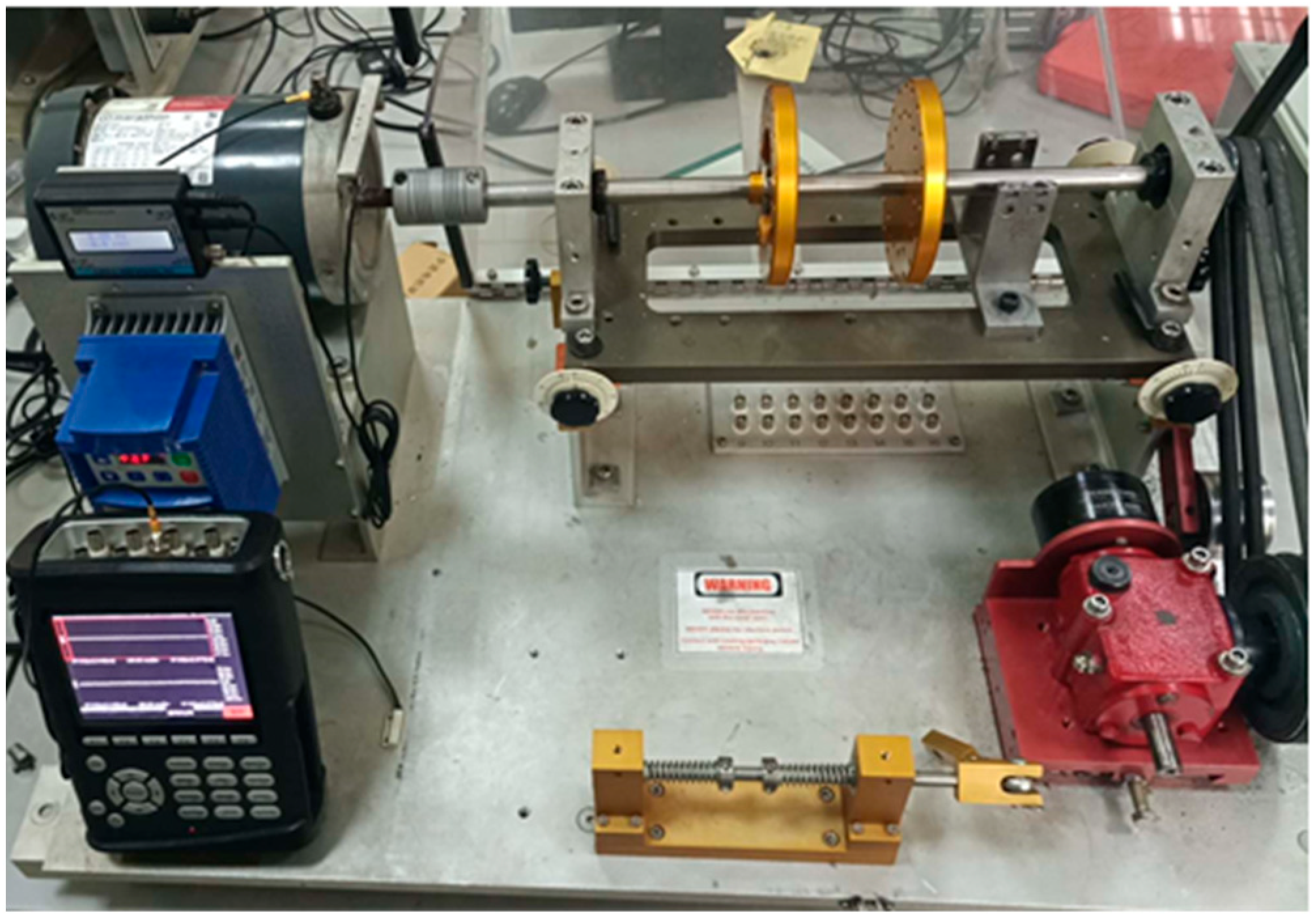
The bearing dataset used for the first case in this study was provided by the CWRU Bearing Data Center and is a highly recognized dataset in the field of bearing fault diagnosis [36]. The test equipment consisted of a 2 HP (1.5 KW) motor, a torque transducer/translator, a power test meter, and an electronic controller. EDM was used to produce different degrees of single-point failures on the ball and inner and outer rings of the bearings. The bearing diameters used for testing were 0.1778 mm, 0.3556 mm, and 0.5334 mm. Acceleration sensors were used for vibration signals collected in the vertical direction from the bearings at the fan end (FE), the drive end (DE), and the housing at the base (BA). Tests were also conducted under four different loads (0–3 HP). The CWRU bearing test platform is shown in Figure 10.
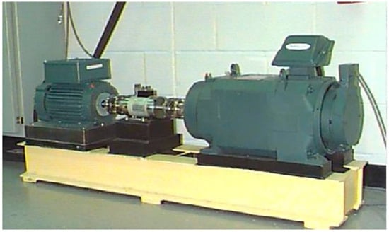
Figure 10.
CWRU test platform.
The vibration signal sampling frequency of the CWRU bearing testing platform is 12 kHz. For this experimental case, we conducted an analysis using the DE bearing data under 0 HP. The bearing speed under this operating condition is 1797 r/min. The experimental data include a normal vibration signal and nine different types of vibration signals with rolling element fault, inner race fault, and outer race fault scenarios using three different diameter bearings and totaling 10 types of bearing vibration signals. The time domain images and the corresponding TF images of the different bearing vibration signals are shown in Figure 11.
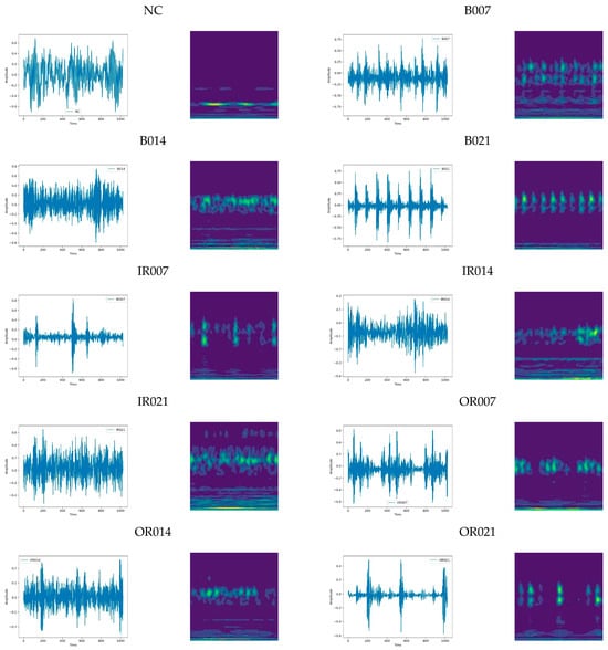
Figure 11.
Different time domain images and corresponding TF images of bearings in the CWRU dataset (0 HP).
Taking the CWRU dataset as an example, by comparing the time domain images and the TF images for each category in Figure 11, we can intuitively see that the smoothness of the vibration signals in the normal category is reflected in the TF image, while the vibration signal characteristics of the fault category are also reflected in the TF images. This observation corroborates the findings of Zhong et al. [37]. It is worth noting that the peaks and valleys of the vibration signals correspond to the irregular shapes in the TF images.
4.1.2. Bearing Data Pre-Processing
The bearing vibration signals used in this case study are those of the drive-end (DE) bearing for determining whether the samples are in normal condition (NC) or whether diagnoses of ball faults (B), inner ring faults (IR), or outer ring faults (OR) can be made. The length of each bearing data sample was 1024, and the original vibration signal samples were augmented using a window sliding method with a window sliding interval of 512. A total of 235 faulty samples and 475 normal samples for each category were obtained. The first 150 samples of each category are chosen for generative model training and the last 80 samples are used for fault diagnosis testing. According to the operation of the bearings in the actual project, most of the samples were normal, while failures occurred in a minority of cases. The bearing fault diagnosis experiments were set up with several S&I task settings for balances of 2:1, 5:1, and 10:1, as well as a normal 1:1 balance for comparison. Table 2 shows the CWRU experimental task design.
Table 2.
CWRU experimental task design.
According to Table 2, we obtained three different proportions of the S&I experimental tasks as well as one sample-balanced experimental task. In the subsequent experiments, we added the samples generated by the WDCGAN-GP to the datasets in the three imbalanced experimental tasks to form a newly balanced hybrid dataset. Finally, we combined the CNN-CA models to perform fault diagnoses.
4.1.3. Quality Assessments and Comparisons of Generated Samples
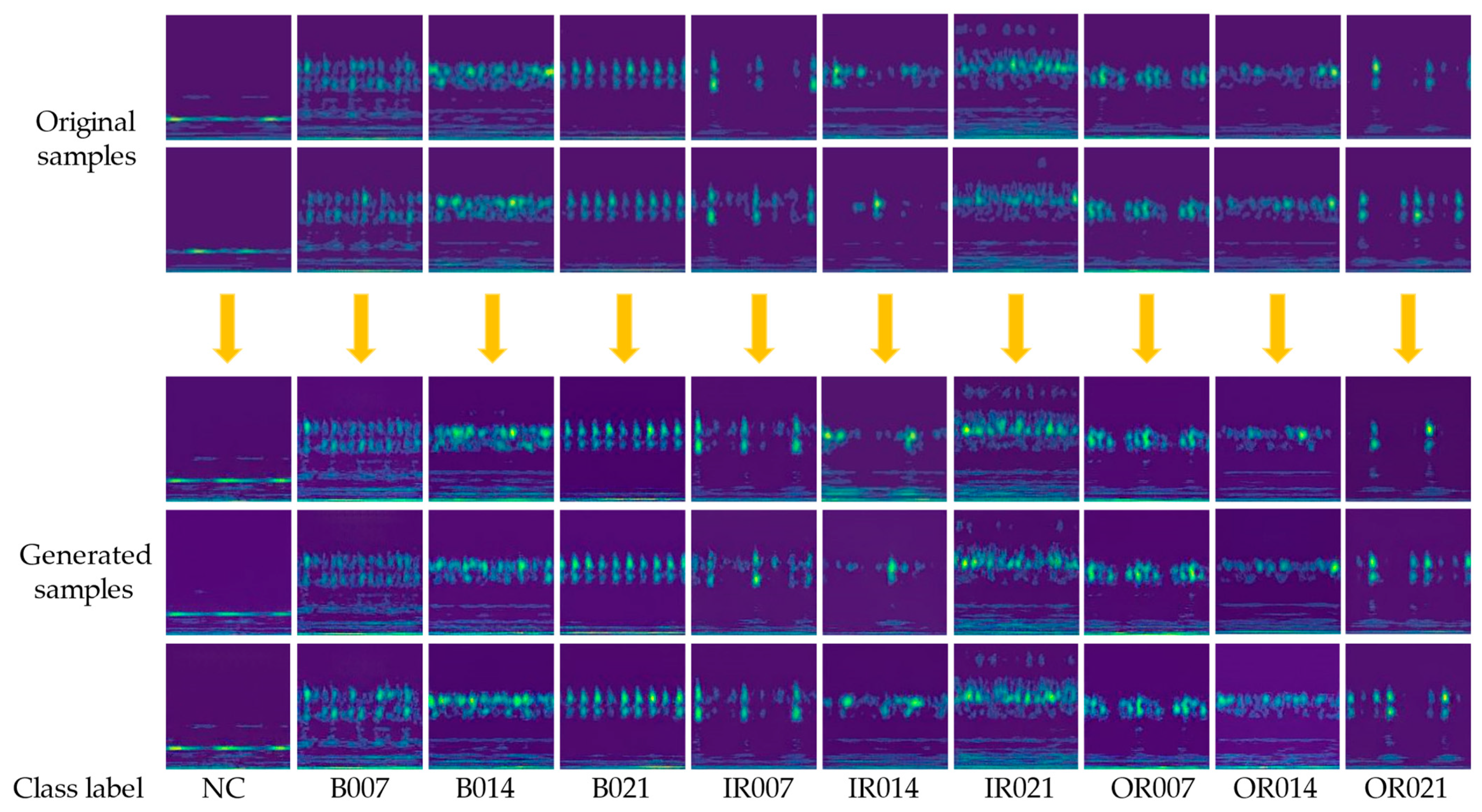
The effectiveness of fault diagnosis is influenced by the quality of the generated TF image. Specifically, in the case of S&I data, if the generated TF samples can accurately reflect the data distribution provided by the original TF image, they can be beneficial for the fault diagnosis model to grasp the data’s features. A comparison between the original TF image samples and the generated ones is shown in Figure 12.

Figure 12.
Comparison of original TF images and the generated TF images for the CWRU dataset.
By comparing the generated TF images to the original ones, it is evident that the WDCGAN-GP can generate new data samples of high quality. In the following, the generated samples are quantitatively analyzed. The feature linkage between the generated samples and the original samples is evaluated using SSIM as well as FID metrics. Ten generated samples are selected for the evaluation of SSIM with the original samples, and the the results of the comparison are averaged to obtain the final result. The FID metric is used to evaluate 150 generated samples as well as the original 150 samples. In addition to the proposed method, this article also compares our model with the generative adversarial network models of the DCGAN and the WGAN-GP, which have the same structure as the WDCGAN-GP. The outcome of this comparison is shown in Table 3.
Table 3.
Evaluation of generation results with different generation models for CWRU dataset.
According to the data in Table 3, we can see that the WDCGAN-GP can generate new high-quality samples and improve both the SSIM and FID metrics compared to the DCGAN and WGAN-GP. By comparing the final evaluation results, we can see that the fault category corresponding to the TF image with a small number of light-colored regions performs better in comparison to the other TF image categories that contain more light-colored regions. Because the location and size of the light-colored regions in the generated samples differ from those of the original TF images, the fault category corresponding to the TF image with more light-colored regions has lower evaluation results compared to those of the other categories.
4.1.4. S&I Fault Diagnosis
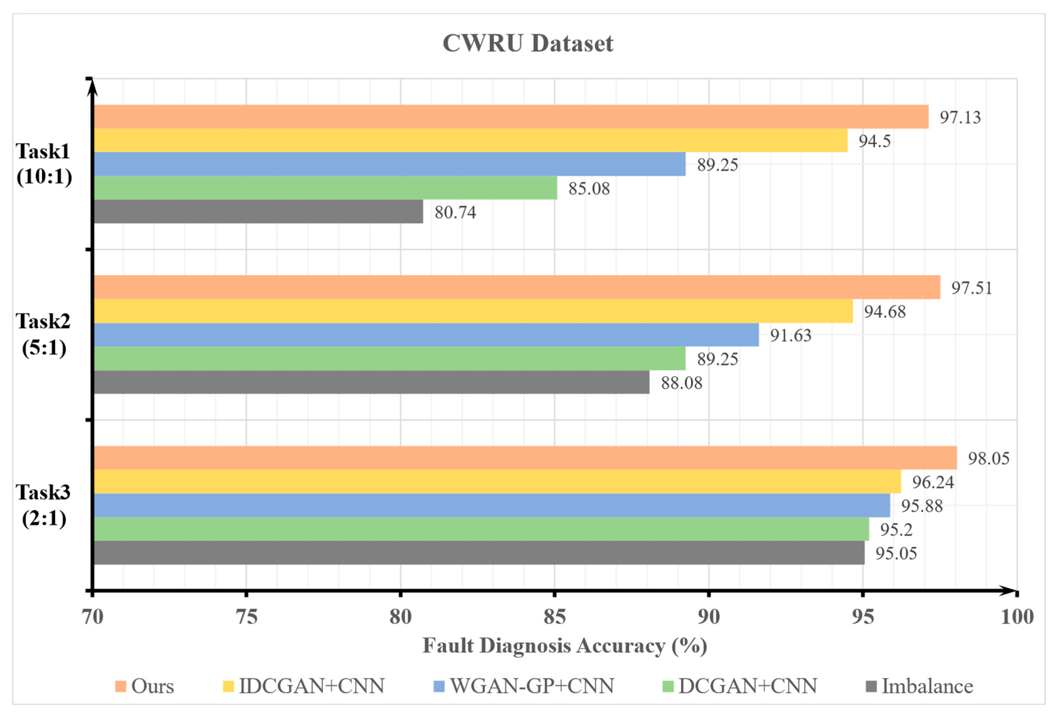
For bearing fault diagnoses in cases of small samples of data and imbalanced data, new TF diagrams are first generated using the WDCGAN-GP and then added to the three S&I datasets sequentially according to the category labels. The number of samples of each category in the balanced dataset is kept at 150. Comparisons were made ten times for each set of experiments, and the average value was taken as the final fault diagnosis result. Tests were performed to enable us to make comparisons after supplementing the original imbalanced dataset with the samples generated by the DCGAN and the WGAN-GP. Fault diagnoses were performed using the CNN and CNN-CA. A comparison of the results of the fault diagnoses using various methods for different experimental tasks is shown in Figure 13.
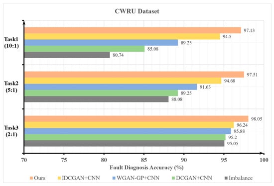
Figure 13.
Comparison of fault diagnosis results using different methods in CWRU dataset.
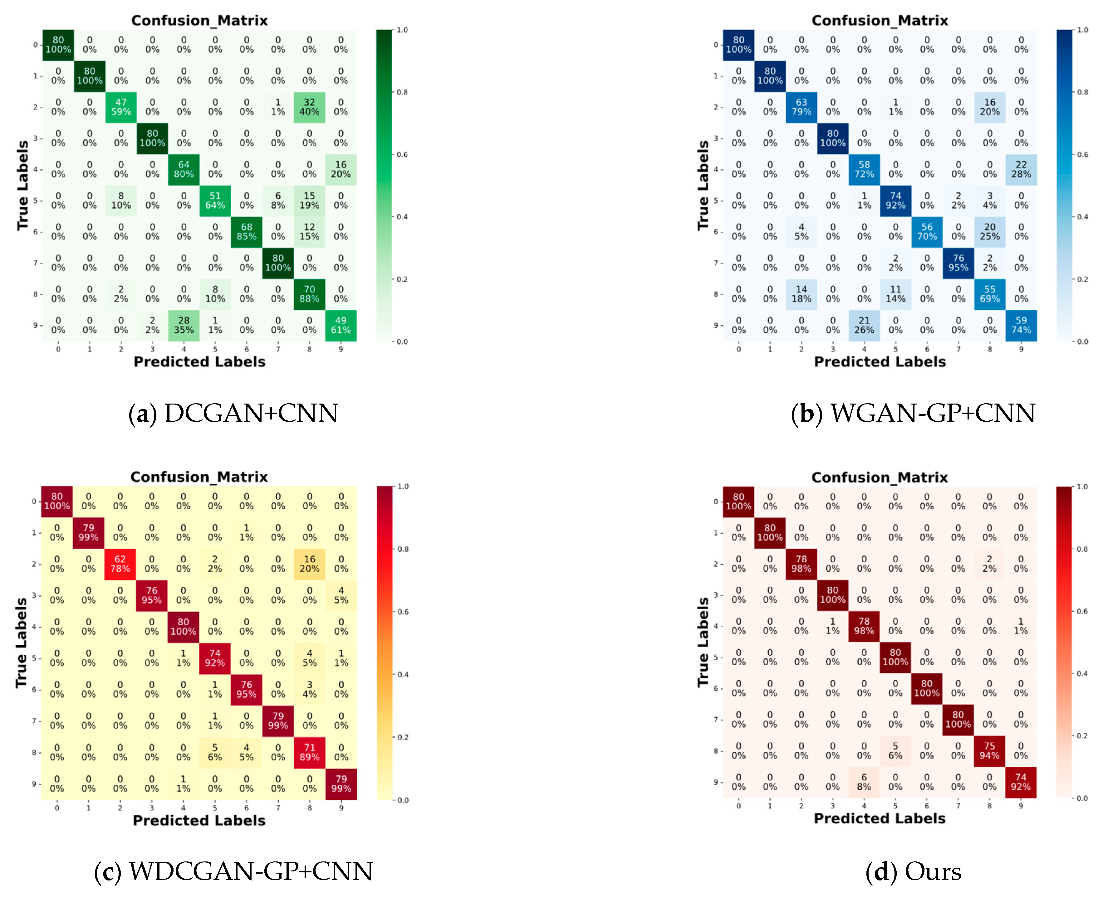
In Figure 13 above, the horizontal axis depicts the precision of fault identification, while the vertical axis represents the various experimental approaches in three distinct S&I scenarios. The results show that in the experimental task with S&I data, the accuracy of fault diagnoses decreases as the imbalance ratio increases. The samples generated by the DCGAN and the WGAN-GP are added to the S&I dataset, respectively, to form a new mixed dataset, which improves the fault diagnosis accuracy compared to that of the original S&I dataset. When the generated samples of the WDCGAN-GP are added and the CNN-CA is used as the fault diagnosis model, the fault diagnosis accuracy is improved compared to that of the other methods and the original. In Task 1, Task 2, and Task 3, the accuracy of the proposed method increases by 16.39%, 9.43%, and 3% compared to that of the original S&I state, respectively. We also validate the experimental task of Task 4 with the aim of comparing the fault diagnoses after the addition of the generated samples in the three S&I tasks to the fault diagnoses in the original balanced state, as well as the performance of the fault diagnosis model of the CNN-CA. The accuracy of the CNN is 96.51% and the accuracy of the CNN-CA is 98.6% when balancing the original samples in Task 4. By adding the CA module, the fault diagnosis accuracy increased by 2.09% compared to the CNN accuracy. The confusion matrix for fault diagnosis and t-distributed stochastic neighbor embedding (t-SNE) visualization [38] can reflect detailed information about the fault categories in the diagnostic results and can also verify the quality of the generated samples and the fault diagnosis performance of the proposed method. The final results reflect the fact that, in the case of an insufficient number original fault data, generated samples can provide reliable data support for fault diagnosis models. The confusion matrix for fault diagnosis and t-SNE visualization for different methods in Task 1 is shown in Figure 14.
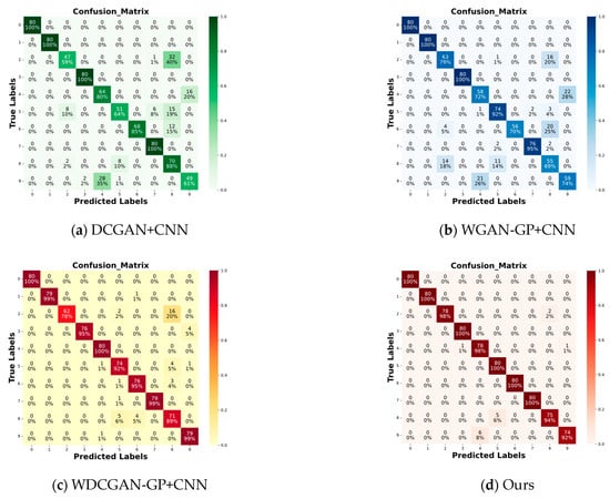
Figure 14.
Comparison of confusion matrices for different methods of fault diagnosis in Task 1.
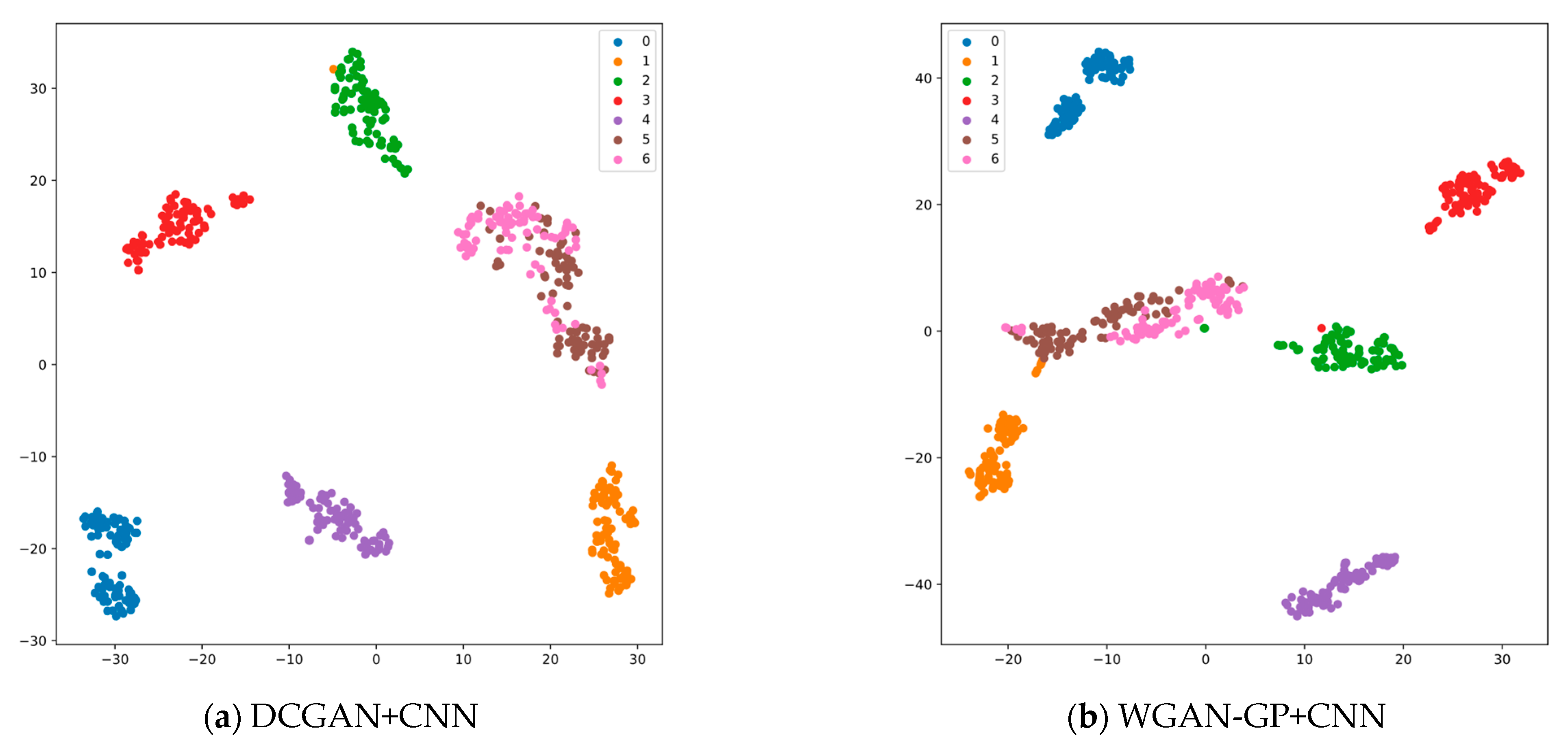
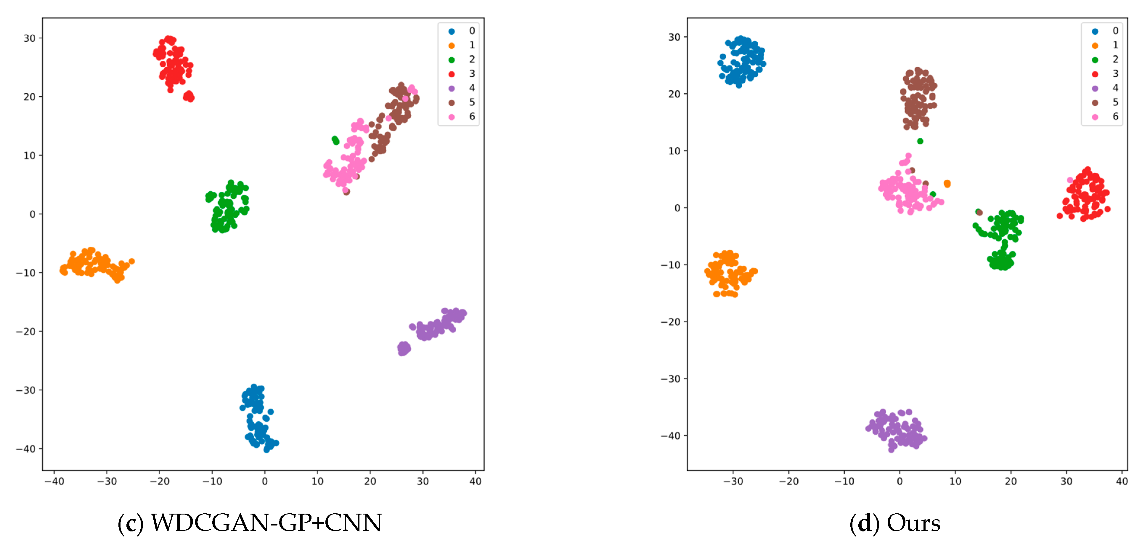
By analyzing Figure 14 and Figure 15, we can see that in the case of Task 1, the proposed fault diagnosis method obtains a high accuracy rate with an average value of 97.13%. However, for some categories of fault classification, it is still insufficient. Fault categories No. 2, No. 5, and No. 8 show relatively poor performances. We tested the rolling element, the inner ring, and the outer ring of 0.3556 mm bearings and also incorporated the confusion matrix as well as the data clustering of the t-SNE visualization. Nevertheless, with the suggested approach, this predicament can be resolved, thereby substantiating the efficacy of the proposed method when applied to scenarios involving S&I data.
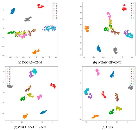
Figure 15.
Comparison of t-SNE for different methods of fault diagnosis in Task 1.
4.2. Experiments with the XJTU-SQ Dataset
4.2.1. Introduction to XJTU-SQ Bearing Data Set
Case 2 of this article utilizes the XJTU-SQ dataset [39,40,41]. This dataset involves the simulation of faults in the inner and outer races of motor bearings using SQ’s comprehensive mechanical fault simulation test platform. The bearings used are NSK 6203 bearings. The bearing faults are artificially created using a grinding pen. The dataset includes normal vibration signals as well as motor bearing vibration signals collected for three different levels of inner race faults and three different levels of outer race faults. The test platform consists of three main components: the motor, the rotor, and the load. Piezoelectric acceleration sensors are used to collect the vibration signals of the motor bearings, with a sensitivity of 50 mv/g. The data acquisition device used is the CoCo80. The signal sampling frequency is 25.6 KHz. In the dataset, the rotation frequency of the bearings with three degrees of failure of the outer ring and a high number of incidences of failure of the inner ring is 19.05 Hz; the rotation frequency of the bearings with a moderate number of incidences of failure of the inner ring is 19.01 Hz; the rotation frequency of the bearings with a low number of incidences of failure of the inner ring is 19.07 Hz; and that of the normal bearings is 19.46 Hz. The XJTU-SQ bearing experimental platform is shown in Figure 16.

Figure 16.
XJTU-SQ bearing test platform.
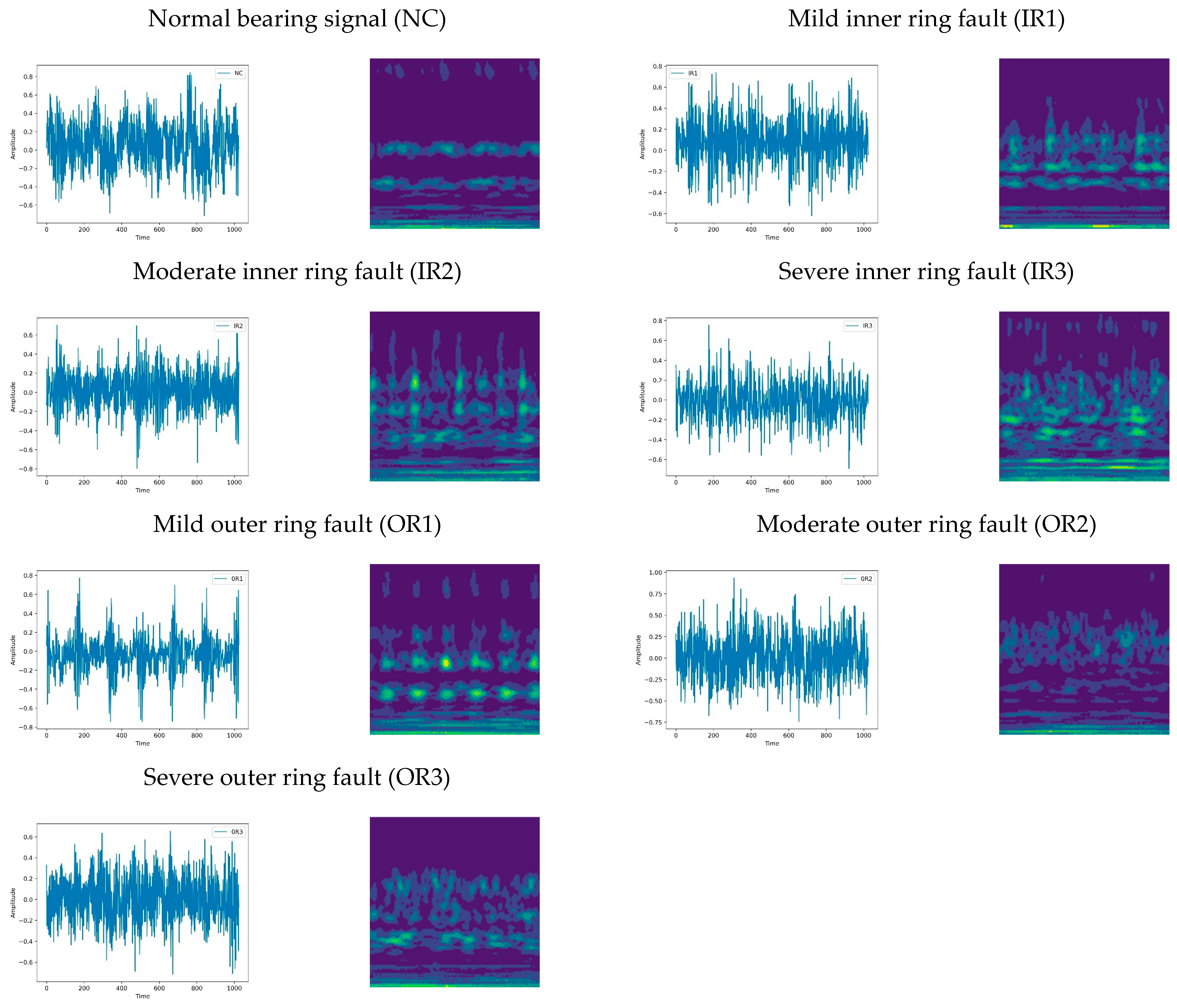
The time domain images and corresponding CWT TF images of the seven different bearing vibration signals in the XJTU-SQ bearing dataset are shown in Figure 17. Each set of images is accompanied by corresponding fault information and labels.
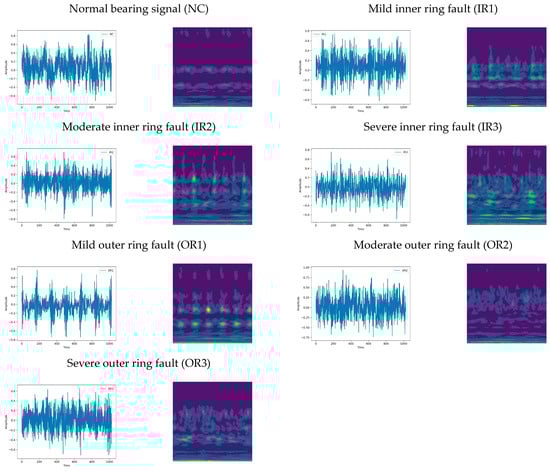
Figure 17.
Different time domain images and corresponding TF images of bearings from XJTU-SQ dataset.
4.2.2. Bearing Data Pre-Processing
The preprocessing method is the same as that used for Case 1. Firstly, the one-dimensional vibration signals are controlled in the interval of [−1, 1] using min–max normalization. The normalized vibration signals are converted to 128 × 128 TF images using CWT. Each TF image contains 1024 data points. The sliding interval of the data points between samples is 512. A total of 400 samples of each type are selected. The first 150 are used for model training and the last 80 are used for fault diagnosis testing. The experimental task settings are consistent with those of Case1, all according to balances of 1:1, 2:1, 5:1, and 10:1. The test set is kept separate from the model training process and is solely utilized for fault classification testing. The case settings are outlined in Table 4 below.
Table 4.
XJTU-SQ experimental task design form.
4.2.3. Quality Assessments and Comparisons of Generated Model
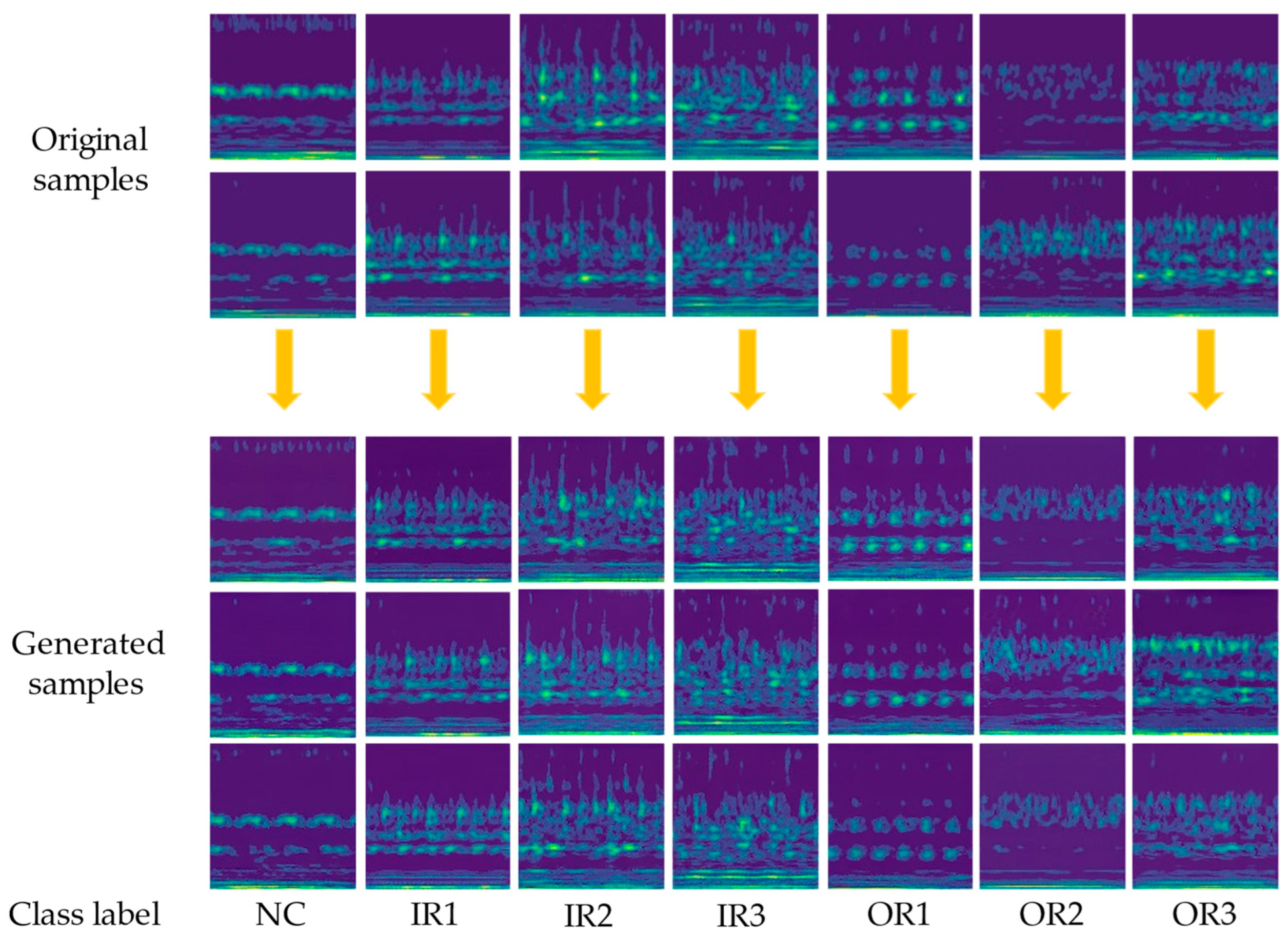
The architecture and parameter aspects of the generated model are the same as those used in Case1. After the training of the WDCGAN-GP finished, the model generated TF image samples that possessed a high degree of similarity to the original TF image samples. The generated results after training are shown in Figure 18.
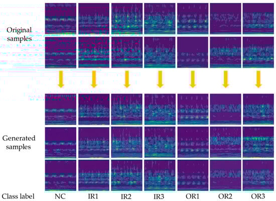
Figure 18.
XJTU-SQ original samples and generated samples.
The quantitative evaluation method of the generated samples of the XJTU-SQ dataset also included the SSIM and FID metrics. To evaluate the quality of the generated samples, 10 samples were randomly selected and compared with the original samples. The average value of the SSIM was calculated as the final result. Additionally, for the FID evaluation, 150 generated samples were used along with 150 original samples. The DCGAN and WGAN-GP were chosen for a comparison of the generated models. The model architectures of the DCGAN and WGAN-GP are consistent with the model of our proposed methodology. The results of the comparison for each fault category are shown in Table 5.
Table 5.
Evaluation of generation results with different generation models for XJTU-SQ dataset.
By comparing the evaluation results using the SSIM and FID metrics in Table 5 above, it can be found that the proposed WDCGAN-GP shows improvements in terms of the quality of the generation of different fault categories compared to that of both the DCGAN and WGAN-GP. In the TF images, different categories of fault signals are represented by distinct regions. The generated samples tend to have more light-colored regions when based on TF images, such as the fault samples labelled as No. 2 and No. 3. They also have lower SSIM values compared to the rest of the categories because although the model can learn the features of the light-colored regions, the light-colored regions in the generated samples may be biased from the original images, which is the same conclusion as that for Case 1.
4.2.4. S&I Fault Diagnosis
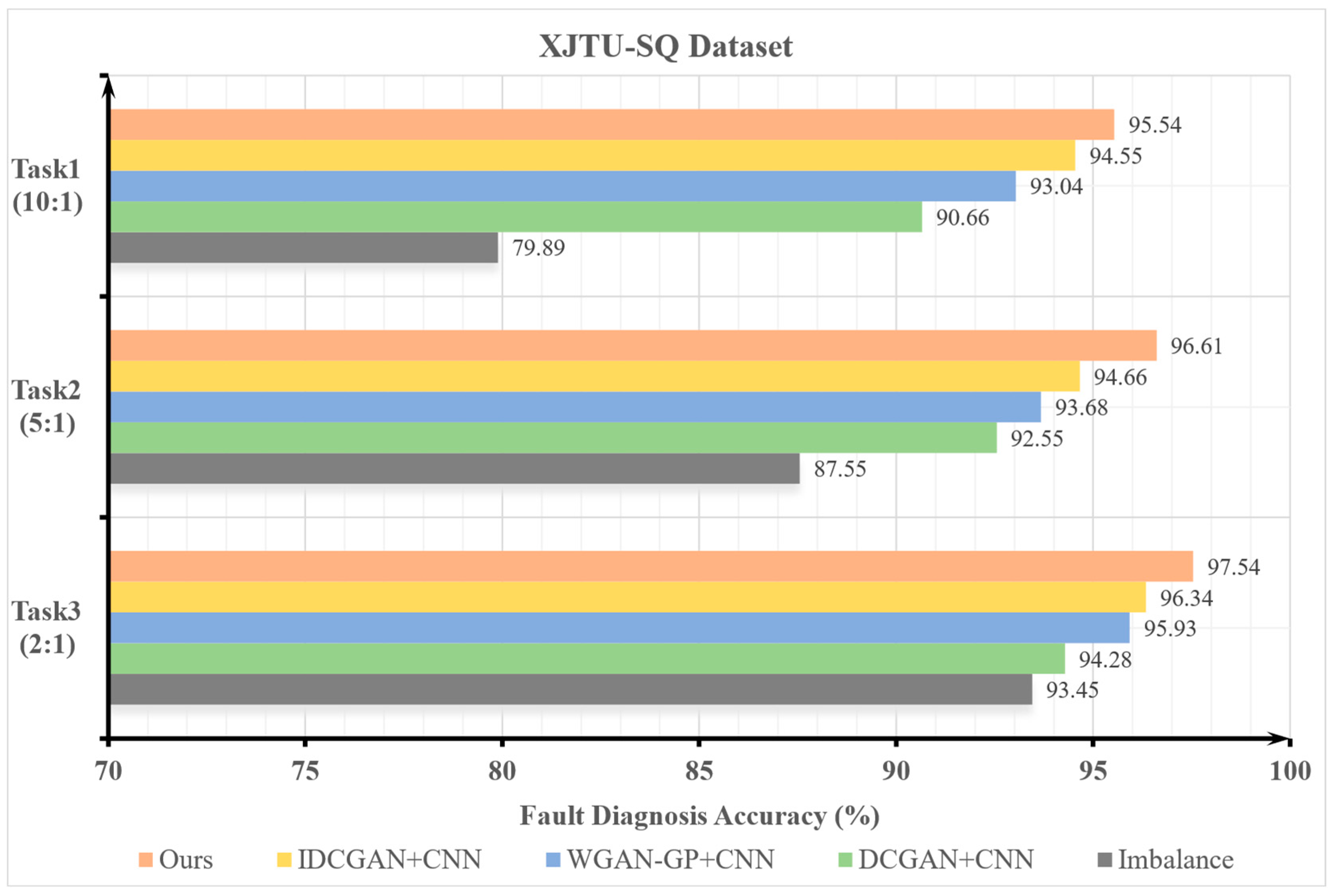
The SSIM and FID metrics evaluate the generated data from an image data perspective. The accuracy of the model classification is discussed as the final evaluation metric of the fault diagnosis method for fault diagnosis applications. According to the three S&I dataset setups shown in Table 4, we generated new samples using the DCGAN and WGAN-GP as well as the proposed method. The classifiers used the CNN and CNN-CA for fault diagnoses of the mixed dataset. The final results are all averaged over ten times to obtain the final fault diagnosis accuracy. The fault diagnosis results for the different scenarios of XJTU-SQ are shown in Figure 19.
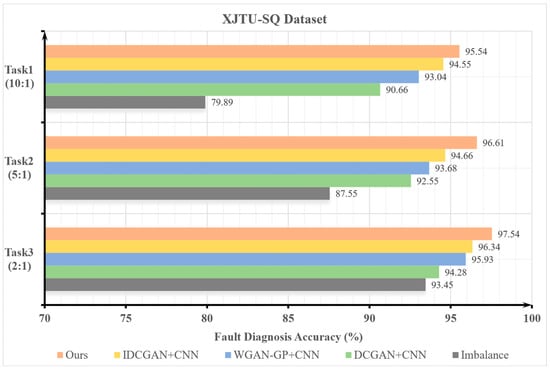
Figure 19.
Comparison of fault diagnosis results using different methods for XJTU-SQ dataset.
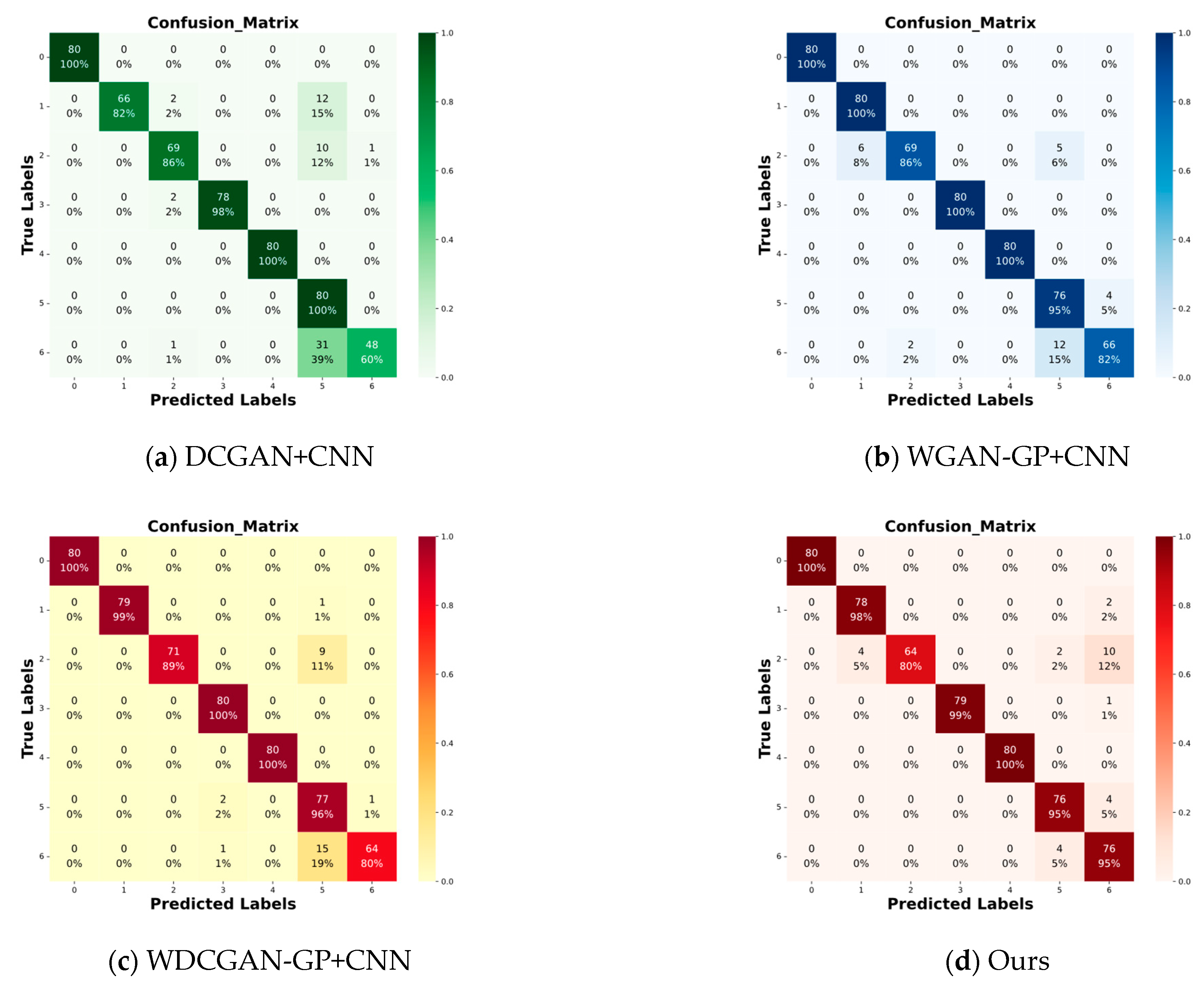
In Figure 19, the x-axis represents the accuracy of classification, and the y-axis represents the experimental methods in the three different cases. The results show that the hybrid dataset generated by several different generation methods improved the diagnostic accuracy compared to the diagnostic accuracy with the S&I data. The proposed method improved the accuracies in Task 1, Task 2, and Task 3 by 15.65%, 9.06%, and 4.09%, respectively, compared to the accuracy with the S&I data. In Task 4, in which the number of bearing categories is balanced, the accuracy of the CNN is 95.86% and that of the CNN-CA is 97.8%. The inclusion of CA increases the fault diagnosis accuracy by 1.94%. Taking Task 1 as an example, the confusion matrix and t-SNE visualization results for the different methods are shown in Figure 20 and Figure 21.
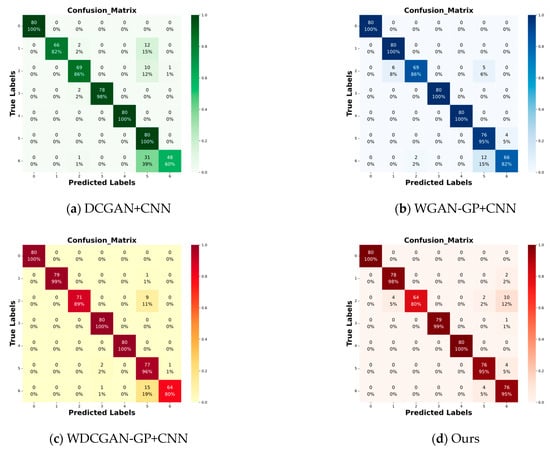
Figure 20.
Comparison of confusion matrices for different methods of fault diagnosis in Task 1.
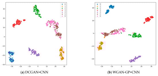
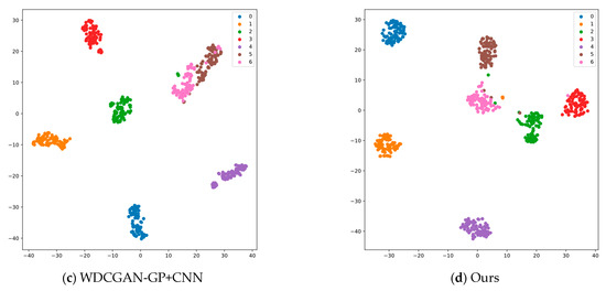
Figure 21.
Comparison of t-SNE for different methods of fault diagnosis in Task 1.
As shown in Figure 20 and Figure 21, the results indicate that the proposed method in this article achieves a satisfactory level of fault diagnosis accuracy in Task 1. Based on the analysis of the confusion matrix for the fault results, it is observed that No. 2 exhibits a poor accuracy in terms of fault diagnosis. This fault type corresponds to a moderate fault in the inner ring of the bearing. This error in fault diagnosis tends to misclassify samples as having fault No. 5. Meanwhile, No. 5 and No. 6 samples are more likely to be clustered together in t-SNE. These fault types are moderate and severe faults of the outer ring of the bearing, and there are a few similarities in the TF image performances of these two types of bearing faults; thus, diagnostic bias occurs in the fault diagnosis results. Finally, the average fault diagnosis accuracy of this article’s method in Task 1 is 95.54%, and our t-SNE results can better distinguish the different categories of fault samples. Thus, it can be verified that the method proposed is effective for the XJTU-SQ dataset.
4.3. Case Comparison Discussion
The proposed method is validated using two distinct bearing datasets. In both cases, the WDCGAN-GP successfully generates higher-quality samples by learning from the original TF images. To highlight the advantages of the proposed model and facilitate observations, we selected three categories with clear periodicity in the vibration signal from each of the two datasets. The differences between the samples generated by the different models are marked with red circles. It is worth noting that the samples compared are randomly selected generated samples from the corresponding categories. A comparison of the generated samples from the different models is shown in Figure 22.
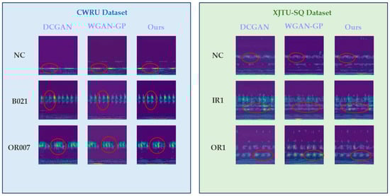
Figure 22.
Comparison of different models’ generated samples.
In the CWRU experimental case, the highest average value of the SSIM evaluation for the generated samples is 0.81. Additionally, the lowest value of the FID metric is 44.5, indicating a close match between the generated samples and the real data distribution. Moreover, the accuracy of the S&I fault diagnosis in the Task 3 experimental task reaches 98.05%. In the experimental case using the XJTU-SQ dataset, the highest SSIM evaluation value of the generated samples is 0.74 and the lowest value of the FID metric is 77.03. Similarly, the accuracy of fault diagnosis in the Task 3 experimental task is up to 97.54%. In both bearing datasets, the accuracy of the proposed method is improved compared to that of fault diagnosis with S&I data. The number of samples generated in both datasets for the normal bearing state is higher than that of the samples for the faulty state, probably because the TF images for the normal operation of the bearings are smaller and more concentrated in terms of energy region compared to the TF diagrams for the faulty state. In addition, in the fault diagnosis of the two datasets, our method shows a small amount of improvement in terms of diagnostic accuracy in Task 3 compared to Task 2 and Task 1, but does not achieve a higher fault accuracy in Task 2 and Task 1, suggesting that the generated samples provide relatively limited data features that can be learnt. There may be some limitations in obtaining higher-accuracy fault diagnoses. In Task 4, the effectiveness of incorporating CA in the CNN was validated under the balanced sample state. The experimental results showed that the accuracy reached 98.6% and 97.8% in Task 4 of the CWRU and XJTU-SQ datasets, respectively. It can be concluded that the CNN-CA has a good level of fault diagnosis accuracy in the experimental task.
5. Conclusions
Aiming at tackling the problems in bearing fault diagnosis in cases with S&I data, this article uses the WDCGAN-GP to enhance fault samples from the perspective of data augmentation. This method is based on the introduction of Wasserstein distance as well as a GP on the basis of the DCGAN, using SN to stabilize the training and adding SA to enhance the learning ability of the network. Finally, the CNN-CA is used as a classification model for fault diagnosis. The proposed method is validated on two different bearing datasets. The fault diagnosis accuracy is improved compared to that of the initial S&I dataset. In Task 1 experimental task, the accuracy of the proposed method is improved by 16.39% and 15.65% compared to the S&I dataset of 80.74% and 79.89%, respectively; therefore, the reliability of the proposed method in this article can be verified.
Although the WDCGAN-GP can generate samples similar to the original images and achieve a high accuracy in fault diagnosis, this method may not be suitable when training data are scarce and single in terms of quantity and categories and when there is an imbalance between fault sample categories. Additionally, the fault data sources used in this study are relatively limited. In the future, we will further explore fault information in vibration signal data and develop multi-source fusion generation models by integrating information from different data sources. This will generate samples with more fault information and better solve the problem of S&I fault diagnosis in industry.
Author Contributions
Conceptualization, Z.Q. and F.H.; methodology, Z.Q. and H.Q.; software and formal analysis, Z.Q. and J.N.; resources, F.H. and J.P.; writing—original draft preparation, Z.Q. and H.Q.; writing—review and editing, F.H. and J.P. All authors have read and agreed to the published version of the manuscript.
Funding
This research received no external funding.
Data Availability Statement
The sources of the data used in this article are linked in the References section. They are publicly available.
Conflicts of Interest
The authors declare no conflicts of interest.
Abbreviations
| S&I | Small & Imbalance |
| GAN | Generative adversarial network |
| DCGAN | Deep convolutional generative adversarial network |
| GP | Gradient penalty |
| WGAN-GP | Wasserstein GAN with GP |
| WDCGAN-GP | Wasserstein DCGAN with GP |
| CNN | Convolutional neural network |
| SN | Spectral normalisation |
| CA | Coordinate attention |
| CNN-CA | Convolutional neural network with CA |
| SSIM | Structural similarity |
| FID | Fréchet inception distance |
| t-SNE | t-distributed stochastic neighbor embedding |
References
- Hakim, M.; Omran, A.A.B.; Ahmed, A.N.; Al-Waily, M.; Abdellatif, A. A systematic review of rolling bearing fault diagnoses based on deep learning and transfer learning: Taxonomy, overview, application, open challenges, weaknesses and recommendations. Ain Shams Eng. J. 2023, 14, 101945. [Google Scholar] [CrossRef]
- Zhou, F.; Yang, S.; Fujita, H.; Chen, D.; Wen, C. Deep learning fault diagnosis method based on global optimization GAN for unbalanced data. Knowl. Based Syst. 2020, 187, 104837. [Google Scholar] [CrossRef]
- Pan, T.; Chen, J.; Xie, J.; Zhou, Z.; He, S. Deep Feature Generating Network: A New Method for Intelligent Fault Detection of Mechanical Systems Under Class Imbalance. IEEE Trans. Ind. Inform. 2021, 17, 6282–6293. [Google Scholar] [CrossRef]
- Ruan, D.; Chen, X.; Gühmann, C.; Yan, J. Improvement of Generative Adversarial Network and Its Application in Bearing Fault Diagnosis: A Review. Lubricants 2023, 11, 74. [Google Scholar] [CrossRef]
- Li, C.; Li, S.; Zhang, A.; He, Q.; Liao, Z.; Hu, J. Meta-learning for few-shot bearing fault diagnosis under complex working conditions. Neurocomputing 2021, 439, 197–211. [Google Scholar] [CrossRef]
- Pan, T.; Chen, J.; Zhang, T.; Liu, S.; He, S.; Lv, H. Generative adversarial network in mechanical fault diagnosis under small sample: A systematic review on applications and future perspectives. ISA Trans. 2022, 128 Pt B, 1–10. [Google Scholar] [CrossRef] [PubMed]
- Zhang, T.; Chen, J.; Li, F.; Zhang, K.; Lv, H.; He, S.; Xu, E. Intelligent fault diagnosis of machines with small & imbalanced data: A state-of-the-art review and possible extensions. ISA Trans. 2022, 119, 152–171. [Google Scholar] [CrossRef] [PubMed]
- Gao, X.; Deng, F.; Yue, X. Data augmentation in fault diagnosis based on the Wasserstein generative adversarial network with gradient penalty. Neurocomputing 2020, 396, 487–494. [Google Scholar] [CrossRef]
- Chen, B.; Tao, C.; Tao, J.; Jiang, Y.; Li, P. Bearing Fault Diagnosis Using ACWGAN-GP Enhanced by Principal Component Analysis. Sustainability 2023, 15, 7836. [Google Scholar] [CrossRef]
- Li, X.; Yue, C.; Liu, X.; Zhou, J.; Wang, L. ACWGAN-GP for milling tool breakage monitoring with imbalanced data. Robot. Comput. Integr. Manuf. 2024, 85, 102624. [Google Scholar] [CrossRef]
- Wen, Q.; Sun, L.; Yang, F.; Song, X.; Gao, J.; Wang, X.; Xu, X. Time Series Data Augmentation for Deep Learning: A Survey. arXiv 2020. [Google Scholar] [CrossRef]
- Wang, H.; Zhu, H.; Li, H. Multi-Mode Data Generation and Fault Diagnosis of Bearings Based on STFT-SACGAN. Electronics 2023, 12, 1910. [Google Scholar] [CrossRef]
- Yang, X.; Liu, B.; Xiang, L.; Hu, A.; Xu, Y. A novel intelligent fault diagnosis method of rolling bearings with small samples. Measurement 2022, 203, 111899. [Google Scholar] [CrossRef]
- Yu, Y.; Guo, L.; Gao, H.; Liu, Y. PCWGAN-GP: A New Method for Imbalanced Fault Diagnosis of Machines. IEEE Trans. Instrum. Meas. 2022, 71, 3515711. [Google Scholar] [CrossRef]
- Pająk, M.; Kluczyk, M.; Muślewski, Ł.; Lisjak, D.; Kolar, D. Ship Diesel Engine Fault Diagnosis Using Data Science and Machine Learning. Electronics 2023, 12, 3860. [Google Scholar] [CrossRef]
- Yang, J.; Liu, J.; Xie, J.; Wang, C.; Ding, T. Conditional GAN and 2-D CNN for Bearing Fault Diagnosis with Small Samples. IEEE Trans. Instrum. Meas. 2021, 70, 3525712. [Google Scholar] [CrossRef]
- Li, W.; Zhong, X.; Shao, H.; Cai, B.; Yang, X. Multi-mode data augmentation and fault diagnosis of rotating machinery using modified ACGAN designed with new framework. Adv. Eng. Inform. 2022, 52, 101552. [Google Scholar] [CrossRef]
- Gu, X.; Yu, Y.; Guo, L.; Gao, H.; Luo, M. CSWGAN-GP: A new method for bearing fault diagnosis under imbalanced condition. Measurement 2023, 217, 113014. [Google Scholar] [CrossRef]
- Li, M.; Zou, D.; Luo, S.; Zhou, Q.; Cao, L.; Liu, H. A new generative adversarial network based imbalanced fault diagnosis method. Measurement 2022, 194, 111045. [Google Scholar] [CrossRef]
- Liang, P.; Deng, C.; Wu, J.; Yang, Z.; Zhu, J.; Zhang, Z. Single and simultaneous fault diagnosis of gearbox via a semi-supervised and high-accuracy adversarial learning framework. Knowl. Based Syst. 2020, 198, 105895. [Google Scholar] [CrossRef]
- Neupane, D.; Kim, Y.; Seok, J. Bearing Fault Detection Using Scalogram and Switchable Normalization-Based CNN (SN-CNN). IEEE Access 2021, 9, 88151–88166. [Google Scholar] [CrossRef]
- Kumar, H.S.; Upadhyaya, G. Fault diagnosis of rolling element bearing using continuous wavelet transform and K-nearest neighbour. Mater. Today Proc. 2023, 92, 56–60. [Google Scholar] [CrossRef]
- Liang, P.; Deng, C.; Wu, J.; Yang, Z. Intelligent fault diagnosis of rotating machinery via wavelet transform, generative adversarial nets and convolutional neural network. Measurement 2020, 159, 107768. [Google Scholar] [CrossRef]
- Goodfellow, I.; Pouget-Abadie, J.; Mirza, M.; Xu, B.; Warde-Farley, D.; Ozair, S.; Courville, A.; Bengio, Y. Generative Adversarial Networks. arXiv 2014. [Google Scholar] [CrossRef]
- Radford, A.; Metz, L.; Chintala, S. Unsupervised Representation Learning with Deep Convolutional Generative Adversarial Networks. arXiv 2015. [Google Scholar] [CrossRef]
- Li, Y.; Zou, W.; Jiang, L. Fault diagnosis of rotating machinery based on combination of Wasserstein generative adversarial networks and long short term memory fully convolutional network. Measurement 2022, 191, 110826. [Google Scholar] [CrossRef]
- Arjovsky, M.; Chintala, S.; Bottou, L. Wasserstein GAN. arXiv 2017. [Google Scholar] [CrossRef]
- Gulrajani, I.; Ahmed, F.; Arjovsky, M.; Dumoulin, V.; Courville, A. Improved Training of Wasserstein GANs. arXiv 2017. [Google Scholar] [CrossRef]
- Miyato, T.; Kataoka, T.; Koyama, M.; Yoshida, Y. Spectral Normalization for Generative Adversarial Networks. arXiv 2018. [Google Scholar] [CrossRef]
- Xu, M.; Wang, Y. An Imbalanced Fault Diagnosis Method for Rolling Bearing Based on Semi-Supervised Conditional Generative Adversarial Network with Spectral Normalization. IEEE Access 2021, 9, 27736–27747. [Google Scholar] [CrossRef]
- Zhang, H.; Goodfellow, I.; Metaxas, D.; Odena, A. Self-Attention Generative Adversarial Networks. arXiv 2018. [Google Scholar] [CrossRef]
- Hou, Q.; Zhou, D.; Feng, J. Coordinate Attention for Efficient Mobile Network Design. arXiv 2017. [Google Scholar] [CrossRef]
- Mi, J.; Ma, C.; Zheng, L.; Zhang, M.; Li, M.; Wang, M. WGAN-CL: A Wasserstein GAN with confidence loss for small-sample augmentation. Expert Syst. Appl. 2023, 233, 120943. [Google Scholar] [CrossRef]
- Shao, H.; Li, W.; Cai, B.; Wan, J.; Xiao, Y.; Yan, S. Dual-Threshold Attention-Guided GAN and Limited Infrared Thermal Images for Rotating Machinery Fault Diagnosis Under Speed Fluctuation. IEEE Trans. Ind. Inform. 2023, 19, 9933–9942. [Google Scholar] [CrossRef]
- Wang, X.; Jiang, H.; Wu, Z.; Yang, Q. Adaptive variational autoencoding generative adversarial networks for rolling bearing fault diagnosis. Adv. Eng. Inform. 2023, 56, 102027. [Google Scholar] [CrossRef]
- Case Western Reserve University. Available online: https://engineering.case.edu/bearingdatacenter/welcome (accessed on 5 February 2024).
- Zhong, Z.; Liu, H.; Mao, W.; Xie, X.; Hao, W.; Cui, Y. Imbalanced Bearing Fault Diagnosis Based on RFH-GAN and PSA-DRSN. IEEE Access 2023, 11, 131926–131938. [Google Scholar] [CrossRef]
- Fan, J.; Yuan, X.; Miao, Z.; Sun, Z.; Mei, X.; Zhou, F. Full Attention Wasserstein GAN with Gradient Normalization for Fault Diagnosis Under Imbalanced Data. IEEE Trans. Instrum. Meas. 2022, 71, 3517516. [Google Scholar] [CrossRef]
- Xi’an Jiaotong University Spectra Quest Bearing Dataset. Available online: https://github.com/Lvhaixin/SQdataset (accessed on 5 February 2024).
- Liu, S.; Chen, J.; He, S.; Shi, Z.; Zhou, Z. Subspace Network with Shared Representation learning for intelligent fault diagnosis of machine under speed transient conditions with few samples. ISA Trans. 2022, 128 Pt A, 531–544. [Google Scholar] [CrossRef]
- Shi, Z.; Chen, J.; Zi, Y.; Zhou, Z. A Novel Multitask Adversarial Network via Redundant Lifting for Multicomponent Intelligent Fault Detection Under Sharp Speed Variation. IEEE Trans. Instrum. Meas. 2021, 70, 3511010. [Google Scholar] [CrossRef]


Disclaimer/Publisher’s Note: The statements, opinions and data contained in all publications are solely those of the individual author(s) and contributor(s) and not of MDPI and/or the editor(s). MDPI and/or the editor(s) disclaim responsibility for any injury to people or property resulting from any ideas, methods, instructions or products referred to in the content. |
© 2024 by the authors. Licensee MDPI, Basel, Switzerland. This article is an open access article distributed under the terms and conditions of the Creative Commons Attribution (CC BY) license (https://creativecommons.org/licenses/by/4.0/).