
New Approach of Normal and Shear Stress Components for Multiple Curvilinear Holes Which Weakened a Flexible Plate

Mathematics Department, Faculty of Sciences, Umm Al-Qura University, Makkah 24227, Saudi Arabia
*
Author to whom correspondence should be addressed.
Symmetry 2024, 16(3), 360; https://doi.org/10.3390/sym16030360
Submission received: 7 February 2024
/
Revised: 12 March 2024
/
Accepted: 14 March 2024
/
Published: 16 March 2024
(This article belongs to the Section Mathematics)
Abstract
:In this article, a thin infinite flexible plate weakened by multiple curvilinear holes is considered. The strength shapes are mapped outside a unit circle with the assistance of particular conformal mapping under certain conditions. The mathematical model that governs the rounded forces of the current physical problem is the boundary value problem of elastic media. This study is applicable to many phenomena throughout nature, like tunnels, caves, and excavations in soil or rock. The Cauchy method for complex variables is used to get the closed forms of Gaursat functions and change the problem to a second-type integrodifferential equation with a Cauchy kernel, which is used for a large area of the contact problems. Then, the normal and shear stress components that act on the model are derived. Afterward, some of the physical applications are studied, and different stress components at specific values in each application are calculated and plotted using Maple 2023.
1. Introduction
There is often more stress concentrated in the vicinity of holes in plate structural components when external loads are applied. To assess the stability and strengthening of the structure, it is crucial to compute the stresses on the edges of the holes precisely. Odishelidze and Criado-Aldeanueva [1] studied axially symmetric problems of the plane theory of elasticity with partially unknown limits, where these problems were studied for a rhombus weakened by one or two holes. Manickam et al. [2] attempted to study the nonlinear thermo-elastic buckling characteristics of composite variable stiffness beams with layers using curvilinear fibers under a thermal environment. Hsieh and Hwu [3] derived a full-field solution for an infinite anisotropic plate containing a hole perturbed from an ellipse subjected to uniform loading at infinity with Stroh formalism. Kaloerov et al. [4] presented a general solution to the problems of elasticity theory for anisotropic half-planes and strips with arbitrary holes and cracks. Li et al. [5] presented a modified Laurent series to investigate the elastic field around holes and inclusions under plane deformation. Akinola [6] emphasized the alternate formulation of the Cauchy–Riemann criteria for the analyticity of a complex variable function. Using the complex variable method, Guo and Lu [7] proposed a new approach to solving the elastic–plastic fields close to the elliptical hole’s major-axis line. Ioakimidis and Theocaris [8] suggested a numerical approach for the solution of Cauchy-type singular integral equations along contours in the complex plane. Strack and Verruijt [9] derived an analytical solution for an energetic tunnel in a flexible half-plane. The half-plane’s surface is stress-free, and the tunnel experiences a defined displacement within its circumference. Li and Fan [10] developed the complex variable technique for the plane elasticity theory of icosahedral quasi-crystals. Yu et al. [11] investigated the linear piezoelastic behavior of one-dimensional (1D) hexagonal quasicrystals using the symmetry operations of point groups. Jiao et al. [12] investigated the Reddy-proposed dual mesh control domain method (DMCDM), which combines the benefits of the finite element approach (variable interpolation) and the finite volume method (a global form of the fulfillment of the governing equations).
Identifying and , two analytic functions of a single complex input , is known to be the equivalent (see [13]) of solving the first and second boundary value problems. These functions have to satisfy the following boundary conditions:
where is a predefined function of stresses for the first boundary value problem with . For the second boundary value problem, is a known function of displacement. If , then the area outside of a closed contour that is infinite can be conformally mapped outside of the unit circle. This concerns the rational mapping function , where and do not go away or become infinite. Both and are complex potential functions of the following forms (see [14]):
and
Several authors, including [14,15,16], have discussed the boundary problems for holed infinite plates. A few of them described the solutions as power series using the Laurent theorem. Another technique for dealing with complex variables is the application of Gaursat functions. They take advantage of the characteristics of the circle or any mapped region of Cauchy integrals outside of a unit circle by using the general rational mapping function . They obtain a solution in the form of two complex functions. Abdou et al. [15] applied the Gaursat functions in the complex variable approach to deduce the first and second types on a limitless plate with two holes that curve. Abdou and Monaquel [17] solved the fundamental problems of an infinite plate with a hole that is weakened by a strong pole in any form using the Cauchy singular technique. Mattei and Lim [18] defined a density basis function on the inclusion’s border using the coordinate system made available by the exterior conformal mapping of the inclusion. To create a closed form of Gaursat functions with variant time, Alhazmi et al. [19] used the complex variables approach and assumed an infinite elastic plate that had two holes weakening it. Leonhardt [20] created a generic formula for designing media that produces perfect invisibility while maintaining geometrical optic precision. Trefethen [21] developed new methods for numerical conformal mapping based on the least-squares fitting on the boundary and rational approximations for solving Dirichlet problems. Caprini [22] discussed a reformulation of QCD perturbation theory as an expansion in terms of a set of nonpower functions of the strong coupling. Kiosak et al. [23] have investigated the conformal mappings of particular quasi-Einstein spaces. Symm [24] presented an integral equation technique for determining the conformal mapping of a given simply connected domain onto the unit circle’s interior. O’Donnell and Rokhlin [25] presented a method for creating conformal mappings from any simply linked region in the complex plane onto the unit disk. Fu et al. [26] obtained the equivalent invariant under a class of conformal mappings between two semi-Riemannian manifolds. Moreover, Ghods et al. [27] applied conformal mapping to create the permeance network for complex-geometry air-gap regions. Mukherjee and Fok [28] presented a novel method for computing the fiber field in a generic artery cross-section by applying conformal maps. The technique relies on finding a rational approximation of the conformal map. Wu et al. [29] proposed a numerical method for the conformal mapping of closed-box girder bridges and applied it to flutter performance prediction, which is crucial for ensuring the safety and sustainability of bridge structures.
In this work, we consider a thin infinite flexible plate with a thickness h weakened by multiple curvilinear holes. The plate is subject to external stress that acts in all directions (see Figure 1). If we ignore any effects related to the physical media surrounding the plate, like temperature, dryness, viscosity, etc., we assume that the stress forces are distributed evenly over the area of the plate, except at the holes. These holes are the important regions of the current study and take different shapes; each one has a physical meaning and a different intensity of effect from the stress forces. The current approach in this work is to reduce the area of energy dissipation, the hole regions, to a finite uniform domain. To accomplish this, we use conformal mapping, which does not vanish or become infinite outside a unit circle. The technique’s idea is to transfer the complex plane, which has curvilinear holes. To achieve this, we use a specific conformal mapping. The conformal mapping technique is tailored to this problem in two dimensions. An algorithm is introduced to compute the conformal map for the chosen boundaries to simply study shapes from the conformal map. We apply the complex variables method with the Cauchy technique to solve the boundary value problem and obtain a closed form of the Gaursat functions. Then, the problem is reduced to the integrodifferential equation of the second type with a Cauchy kernel. Moreover, the normal and shear stress components are derived. After that, we explain different physical applications, and then the normal and shear stress components for each one at the chosen values are calculated and plotted using the Maple 2023 software. Finally, the main results of the work are discussed.
2. Basic Equations
In the given area, the boundary S is in the z-plane and is occupied by the plate’s center plane. This boundary is mapped onto the unit circle in the -plane by the rational mapping . Using the formula , curvilinear coordinates are introduced as maps of the polar conditions into the z-plane. The following result is obtained when we apply to (1):
In the -plane, the first and second boundary value problems are represented by Formula (4). The related formulas of (1) are as follows:
where the applied stresses, denoted as and , are defined on the edge of the plane; the displacement variables are p and q, the length is s, and the modulus of shear is G. In addition, the following conditions must be fulfilled by the applied stresses and :
In elastic problems of the plate, the stress components are given by
3. Conformal Mapping and Special Cases
We consider an infinitely thin plate with a curvilinear hole S whose origin is outside the unit circle in the -plane with a rational mapping function
where does not become infinite or vanish, are complex numbers, and are real numbers.
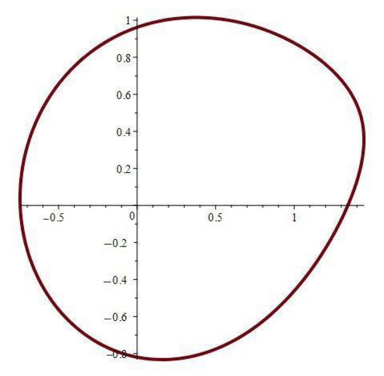
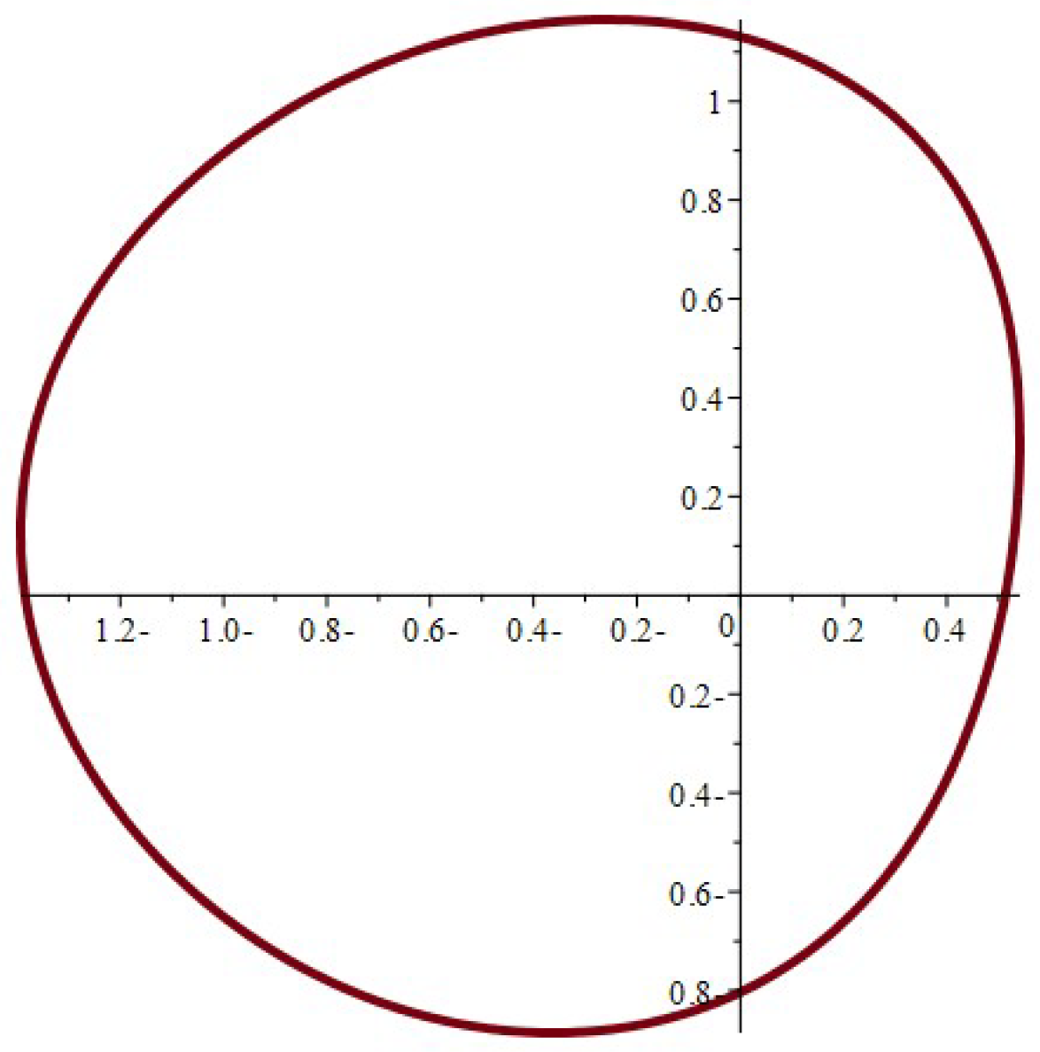
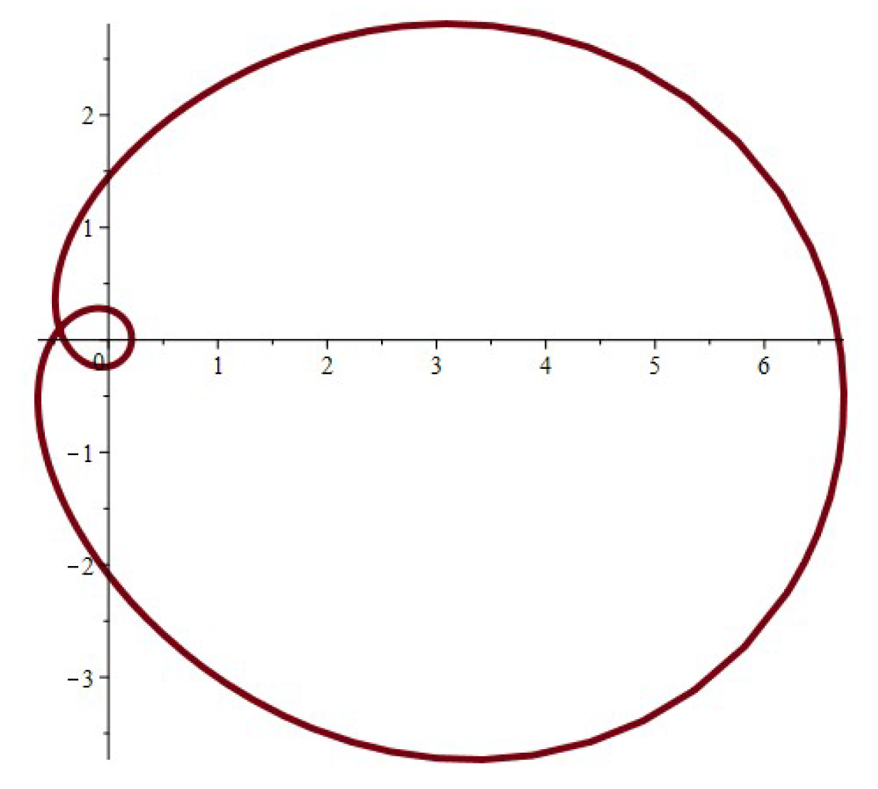
The study focused on normal and shear stress components for flexible plates, which were weakened by curvilinear holes conformally mapped on the domain outside a unit circle by the rational function (10). The physical interest of mapping comes from the different shapes of holes it treats, as shown in Figure 2, Figure 3, Figure 4, Figure 5, Figure 6, Figure 7, Figure 8, Figure 9, Figure 10, Figure 11, Figure 12 and Figure 13.
Special Cases:
- i.
- ii.
- iii.
4. The Method of Solution
The complex Gaursat functions, and , are derived using the complex variable technique (see [30,31]). Furthermore, after determining the Gaursat functions, the three stress components, , , and , will be completely determined. With the boundary condition (1) and the conformal mapping (4), the expression yields
where is a regular function, and
with
where
for and . By virtue of (2), (3), and (11), the condition at the boundary (4) is
where denotes the value on the edge of the unit circle,
and
with
and
The Hölder condition (see [32]) is thought to be satisfied by the function and its derivatives. Our aim is to use the mapping to obtain the functions and for various boundary value problems. To achieve this, we multiply both sides of this mapping by . Then, we integrate the resulting integrals using residue theorems. Thus, we obtain
where
and
Using (11) in the integral term of (15), we assume
where the complex constants ’s are yet to be found. Therefore, we have
Differentiating (18) with respect to and using the result from (17), we obtain
The general solution of (19) is
where
and
From the boundary condition (14), can be determined in the form
where
and
Using (18) in (9), after some derivatives and algebraic relations, we have
where
and
5. Applications
In this section, we resolve the first and second boundary value problems by assuming various values for the given functions. In this case, the Gaursat functions will then be obtained, allowing for the direct calculation of the stress components.
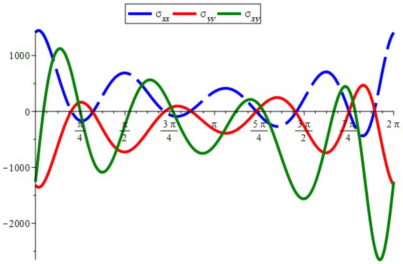
Application 1: A curvilinear hole with uniform tensile stress on an infinite plate: There is an applied uniform tensile tension of intensity P to an infinite plate, stretching it to infinity and forming an angle with the x-axis in the given conditions: , and . The two complex functions of (19) and (21) result in the plate becoming weaker due to a curvilinear hole S that is not under any stress:
where
and
Using (25) and (26) in (23), it is possible to obtain the stress components directly. Figure 14, Figure 15, Figure 16, Figure 17, Figure 18 and Figure 19 show the equations that relate these stress components to the angle .
Application 2: A two-pole curvilinear hole with a uniformly pressured edge: In the case of , and , where P is a real constant, the Equations (19) and (21) become
Hence, when a constant pressure of P is applied to the hole’s edge, Equations (27) and (28) provide the solution to the first boundary value problem. On the other hand, when the edge is under a uniform tangential stress of T, as stated in (27) and (28), we replace P with in (27) and (28).
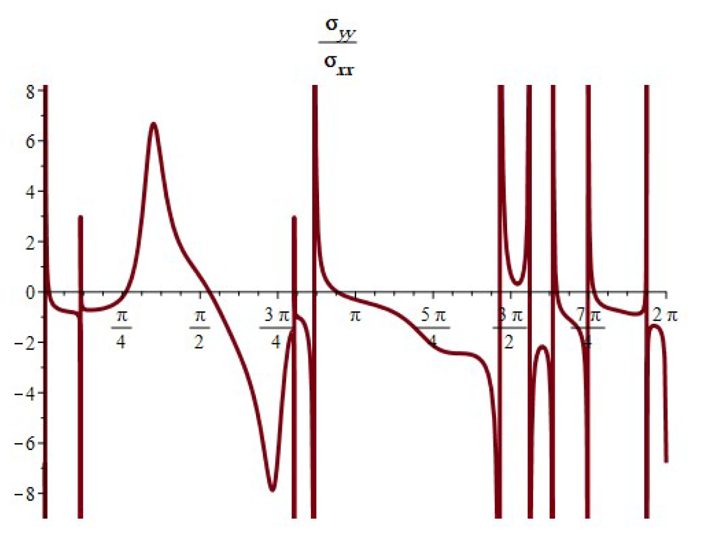
Figure 20, Figure 21, Figure 22, Figure 23, Figure 24 and Figure 25 show the equations relating the stress components to the angle .
Application 3: The curvilinear hole’s center is where the force acts. We assume that the strains, in this case, finish at infinity. The kernel’s lack of rotation is immediately apparent. The kernel usually stays in its original location. Consequently, the Gaursat functions are determined by assuming that and . Thus,
and
where
As a result, the second boundary value problem is resolved, where the curvilinear kernel’s center is subject to a force .
6. Conclusions
In this work, we examined a thin infinite flexible plate with a thickness h weakened by multiple curvilinear holes. There was external stress acting in all directions on the plate. The stress forces are distributed uniformly throughout the plate, except for the edges of the holes, and we disregarded any effects associated with the physical medium surrounding the plate. These holes, which were the focal point of the present investigation, came in various forms, and each had a distinct physical significance and a varying degree of stress force impact. The area of energy dissipation, or the hole area, was reduced to a limited uniform domain using the present methodology; we achieved this by using a certain conformal mapping , where c > 0 to provide the solution to the boundary value problem as a discontinuous kernel integrodifferential equation. This kind of integrodifferential equation plays a famous role in many important applications of contact problems in elastic media and material engineering sciences; see [33,34,35]. The Cauchy technique is a powerful tool that allows us to simplify the singular or super-strong singular problem, enabling us to handle it more efficiently. After obtaining the two Gaursat functions, , , the components of normal and shear stress were determined. The theoretical knowledge is explained, applicably, by the chosen applications in Section 5, as follows:
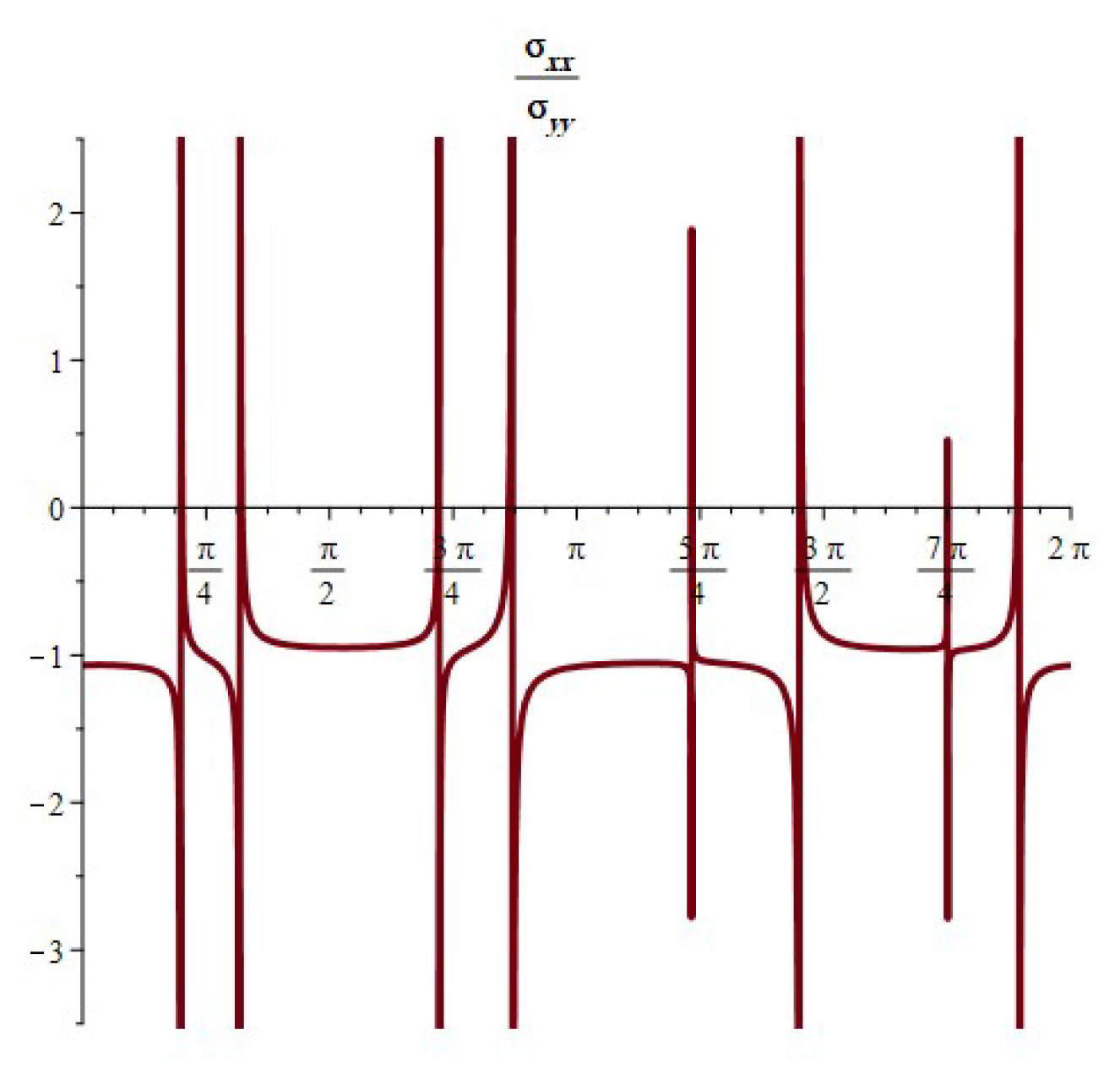
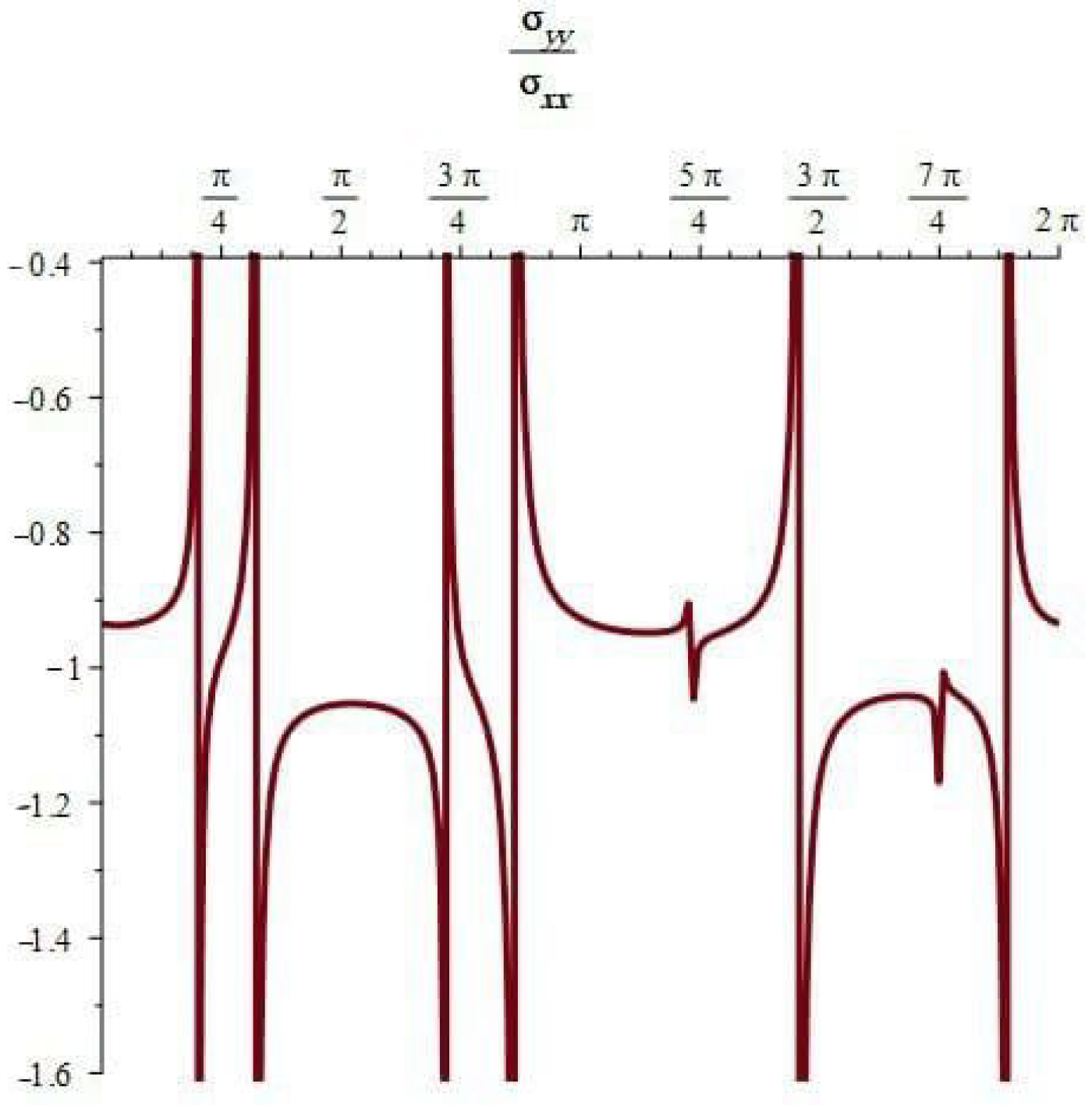
- When , the component of the stress acts as a tensile force. The normal and shear stress component take the shapes of nonhomogeneous waves and form an angle with the x-axis; see Figure 14, Figure 23 and Figure 26. Furthermore, the stress ratio and represents the uniform oscillation; see Figure 15, Figure 16, Figure 24, Figure 25, Figure 27 and Figure 28.
- When , the component of the stress acts as a compression force. The normal and shear stress component take the shapes of compressed interfering waves and form an angle with the x-axis; see Figure 17, Figure 20 and Figure 29. Furthermore, the stress ratio and represents a compressed oscillation; see Figure 18, Figure 19, Figure 21, Figure 22, Figure 30 and Figure 31.
Future Work:
- Study the physical model when the complex potential functions are functions of time. Also, study it in the presence of external forces like flowing heat or a normal magnetic field.
- Study the anomaly model as an application in the medical field. For example, osteoporosis is characterized by a reduction in bone tissue volume and thickness. This causes the bones to weaken and break more easily. Another example is sickle cell anemia, an inherited condition in which red blood cells have an irregular crescent shape, block small blood vessels, and live a shorter life than normal red blood cells.
Author Contributions
Conceptualization, F.M.A.; Methodology, F.M.A. and N.G.A.; Software, N.G.A.; Validation, N.G.A.; Writing—original draft, N.G.A.; Writing—review & editing, N.G.A.; Supervision, F.M.A.; Project administration, F.M.A.; Funding acquisition, F.M.A. All authors have read and agreed to the published version of the manuscript.
Funding
This research received no external funding.
Data Availability Statement
Data are contained within the article.
Conflicts of Interest
The authors declare that they have no conflicts of interest.
References
- Odishelidze, N.; Criado-Aldeanueva, F. Some axially symmetric problems of the theory of plane elasticity with partially unknown boundaries. Acta Mech. 2008, 199, 227–240. [Google Scholar] [CrossRef]
- Manickam, G.; Haboussi, M.; D’Ottavio, M.; Kulkarni, V.; Chettiar, A.; Gunasekaran, V. Nonlinear thermo-elastic stability of variable stiffness curvilinear fibres based layered composite beams by shear deformable trigonometric beam model coupled with modified constitutive equations. Int. J. Non-Linear Mech. 2023, 148, 104303. [Google Scholar] [CrossRef]
- Hsieh, M.-L.; Hwu, C. A full field solution for an anisotropic elastic plate with a hole perturbed from an ellipse. Eur. J. Mech. A Solids 2023, 97, 104823. [Google Scholar] [CrossRef]
- Kaloerov, S.; Glushankov, E.; Mironenko, A. Solution of problems of elasticity theory for multiply connected half-planes and strips. Mech. Solids 2023, 58, 1063–1075. [Google Scholar] [CrossRef]
- Li, C.; Huang, C.; Wang, S.; Cai, D. A modified laurent series for hole/inclusion problems in plane elasticity. Z. Angew. Math. Phys. 2021, 72, 124. [Google Scholar] [CrossRef]
- Akinola, A. On complex variable method in finite elasticity. Appl. Math. 2009, 1, 1–16. [Google Scholar] [CrossRef]
- Guo, J.; Lu, Z. Line field analysis and complex variable method for solving elastic-plastic fields around an anti-plane elliptic hole. Sci. China Phys. Mech. Astron. 2011, 54, 1495–1501. [Google Scholar] [CrossRef]
- Ioakimidis, N.I.; Theocaris, P.S. On a method of numerical solution of a plane elasticity problem. Stroj. Cas. 1978, 29, 448–455. [Google Scholar]
- Strack, O.; Verruijt, A. A complex variable solution for a deforming buoyant tunnel in a heavy elastic half-plane. Int. J. Numer. Anal. Methods Geomech. 2002, 26, 1235–1252. [Google Scholar] [CrossRef]
- Li, L.; Fan, T. Complex variable method for plane elasticity of icosahedral quasicrystals and elliptic notch problem. Sci. China Ser. G: Phys. Mech. Astron. 2008, 51, 773–780. [Google Scholar] [CrossRef]
- Yu, J.; Guo, J.; Xing, Y. Complex variable method for an anti-plane elliptical cavity of one-dimensional hexagonal piezoelectric quasicrystals. Chin. J. Aeronaut. 2015, 28, 1287–1295. [Google Scholar] [CrossRef]
- Jiao, Z.; Heblekar, T.; Wang, G.; Xu, R.; Chen, W.; Reddy, J. Analysis of plane elasticity problems using the dual mesh control domain method. Comput. Methods Appl. Mech. Eng. 2023, 416, 116342. [Google Scholar] [CrossRef]
- Abdou, M. First and second fundamental problems for an elastic infinite plate with a curvilinear hole. Alex. Eng. J. 1994, 33, 227–233. [Google Scholar]
- Abdou, M. Fundamental problems for infinite plate with a curvilinear hole having finite poles. Appl. Math. Comput. 2002, 125, 79–91. [Google Scholar] [CrossRef]
- Abdou, M.; Ibrahim, E.; Basseem, M. The stress and strain components for a weakened elastic plate by two curvilinear holes in presence of heat. Curr. Sci. Int. 2022, 11, 199–216. [Google Scholar]
- Abdou, M.; Khamis, A. On a problem of an infinite plate with a curvilinear hole having three poles and arbitrary shape. Bull. Calcutta Math. Soc. 2000, 92, 313–326. [Google Scholar]
- Abdou, M.; Monaquel, S. Integro differential equation and fundamental problems of an infinite plate with a curvilinear hole having strong pole. Int. J. Contemp. Math. Sci. 2011, 6, 199–208. [Google Scholar]
- Mattei, O.; Lim, M. Explicit analytic solution for the plane elastostatic problem with a rigid inclusion of arbitrary shape subject to arbitrary far-field loadings. J. Elasticity 2021, 144, 81–105. [Google Scholar] [CrossRef]
- Alhazmi, S.E.; Abdou, M.; Basseem, M. The stresses components in position and time of weakened plate with two holes conformally mapped into a unit circle by a conformal mapping with complex constant coefficients. AIMS Math. 2023, 8, 11095–11112. [Google Scholar] [CrossRef]
- Leonhardt, U. Optical conformal mapping. Science 2006, 312, 1777–1780. [Google Scholar] [CrossRef]
- Trefethen, L.N. Numerical conformal mapping with rational functions. Comput. Methods Funct. Theory 2020, 20, 369–387. [Google Scholar] [CrossRef]
- Caprini, I. Conformal mapping of the borel plane: Going beyond perturbative qcd. Phys. Rev. D 2020, 102, 054017. [Google Scholar] [CrossRef]
- Kiosak, V.; Savchenko, A.; Gudyreva, O. On the conformal mappings of special quasi-einstein spaces. AIP Conf. Proc. 2019, 2164, 040001. [Google Scholar] [CrossRef]
- Abdou, M.; Khar-El din, E.A. An infinite plate weakened by a hole having arbitrary shape. J. Comput. Appl. Math. 1994, 56, 341–351. [Google Scholar] [CrossRef]
- O’Donnell, S.; Rokhlin, V. A fast algorithm for the numerical evaluation of conformal mappings. SIAM J. Sci. Statist. Comput. 1989, 10, 475–487. [Google Scholar] [CrossRef]
- Fu, F.; Yang, X.; Zhao, P. Geometrical and physical characteristics of a class of conformal mappings. J. Geom. Phys. 2012, 62, 1467–1479. [Google Scholar] [CrossRef]
- Ghods, M.; Faiz, J.; Gorginpour, J.; Bazrafshan, M.A.; Nøland, J.K. Equivalent magnetic network modeling of variable-reluctance fractional-slot v-shaped vernier permanent magnet machine based on numerical conformal mapping. IEEE Trans. Transp. Electr. 2023, 9, 3880–3893. [Google Scholar] [CrossRef]
- Mukherjee, A.; Fok, P.-W. A new approach to calculating fiber fields in 2d vessel cross sections using conformal maps. Math. Biosci. Eng. 2023, 20, 3610–3623. [Google Scholar] [CrossRef]
- Wu, L.; Zhou, Z.; Zhang, J.; Zhang, M. A numerical method for conformal mapping of closed box girder bridges and its application. Sustainability 2023, 15, 6291. [Google Scholar] [CrossRef]
- Brociek, R.; Pleszczyński, M. Comparison of Selected Numerical Methods for Solving Integro-Differential Equations with the Cauchy Kernel. Symmetry 2024, 16, 233. [Google Scholar] [CrossRef]
- Zhou, Y.; Lin, Y. Solving integro-differential equations with Cauchy kernel. Appl. Math. Comput. 2009, 215, 2438–2444. [Google Scholar] [CrossRef]
- Stein, E.M.; Shakarchi, R. Functional Analysis: Introduction to Further Topics in Analysis; Princeton University Press: Princeton, NJ, USA, 2011; Available online: https://books.google.com.sa/books?id=OUaU-W-dpA0C (accessed on 22 August 2011).
- Althubiti, S.; Mennouni, A. A Novel Projection Method for Cauchy-Type Systems of Singular Integro-Differential Equations. Mathematics 2022, 10, 2694. [Google Scholar] [CrossRef]
- Jan, A.R.; Abdou, M.A.; Basseem, M. A Physical Phenomenon for the Fractional Nonlinear Mixed Integro-Differential Equation Using a Quadrature Nystrom Method. Fractal Fract. 2023, 7, 656. [Google Scholar] [CrossRef]
- Assanova, A.T.; Nurmukanbet, S.N. A Solvability of a Problem for a Fredholm Integro-Differential Equation with Weakly Singular Kernel. Lobachevskii J. Math. 2022, 43, 182–191. [Google Scholar] [CrossRef]
Figure 1.
Three different holes in an infinite plate.
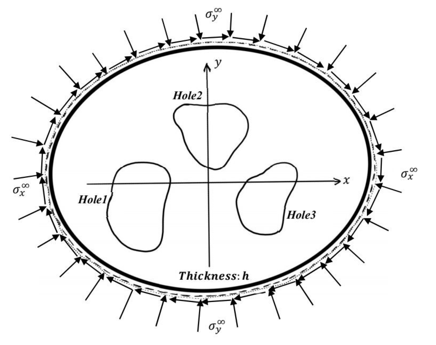
Figure 2.
= , = , .

Figure 3.
.

Figure 4.
.

Figure 5.
.

Figure 6.
.
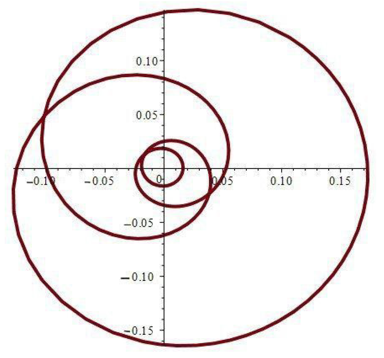
Figure 7.
.
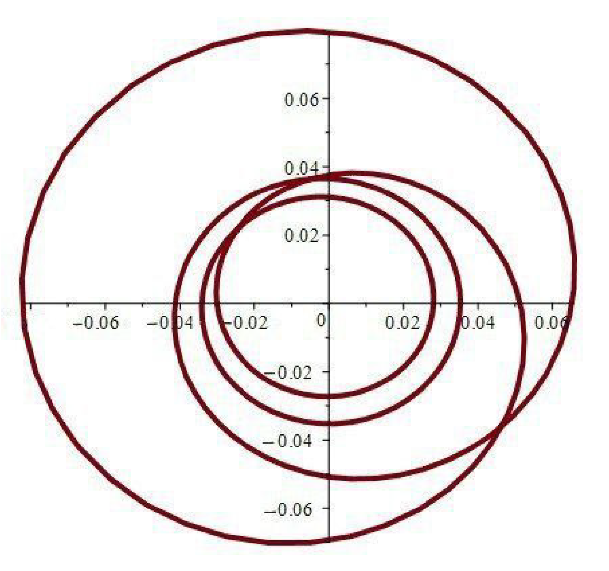
Figure 8.
.

Figure 9.
.

Figure 10.
.
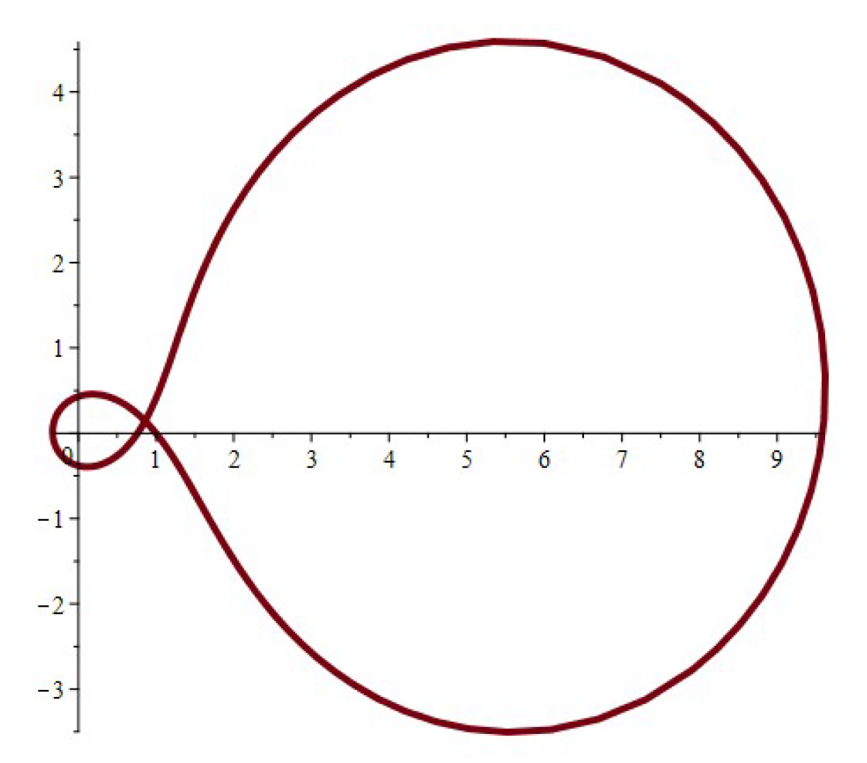
Figure 11.
.
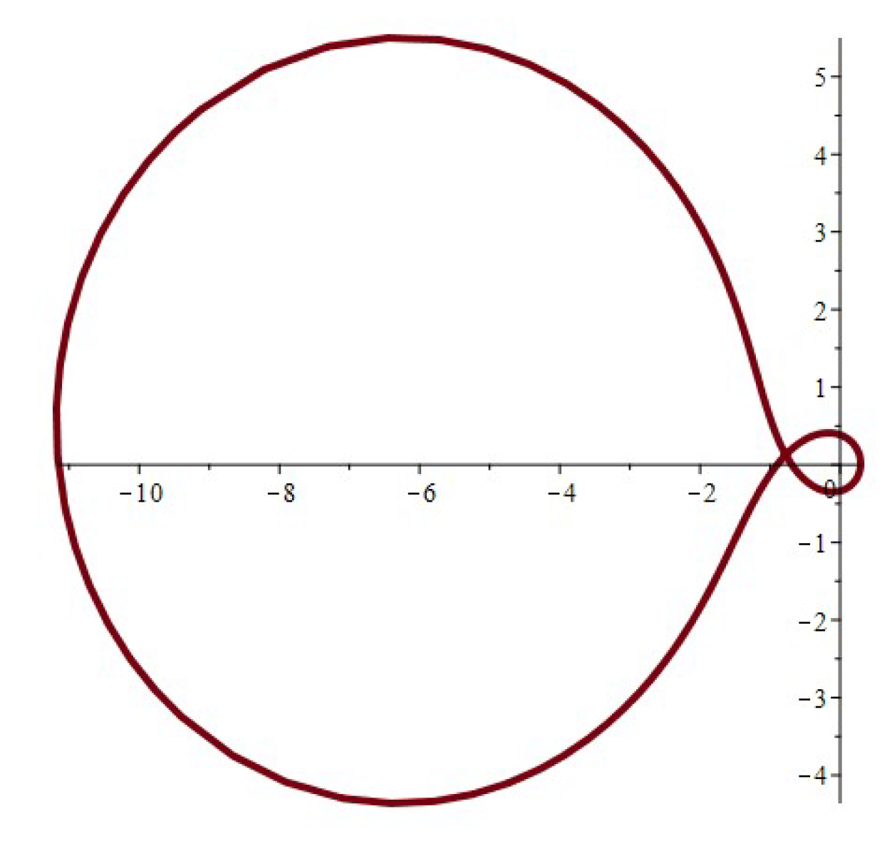
Figure 12.
.

Figure 13.
.

Figure 14.
The relation between stress components and the angle .

Figure 15.
Stress ratio where .

Figure 16.
Stress ratio where .

Figure 17.
The relation between stress components and the angle .

Figure 18.
Stress ratio where .

Figure 19.
Stress ratio where .

Figure 20.
The relation between stress components and the angle .

Figure 21.
Stress ratio where .
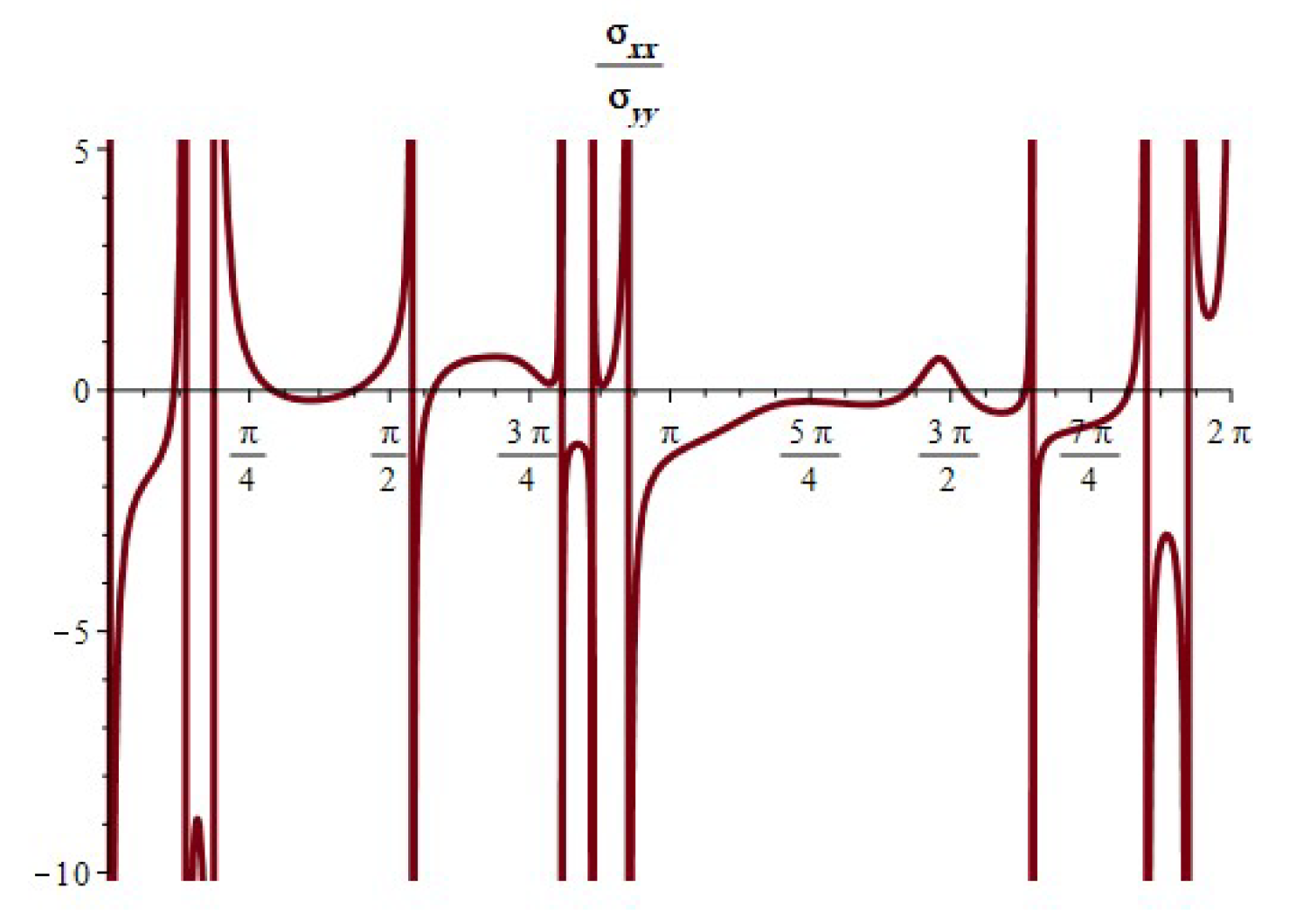
Figure 22.
Stress ratio where .
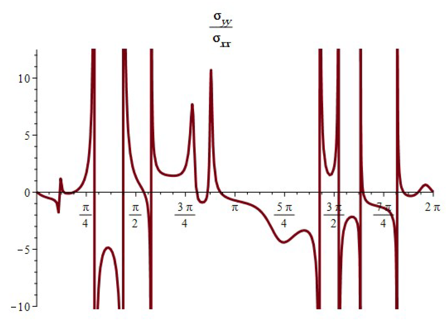
Figure 23.
The relation between stress components and the angle .
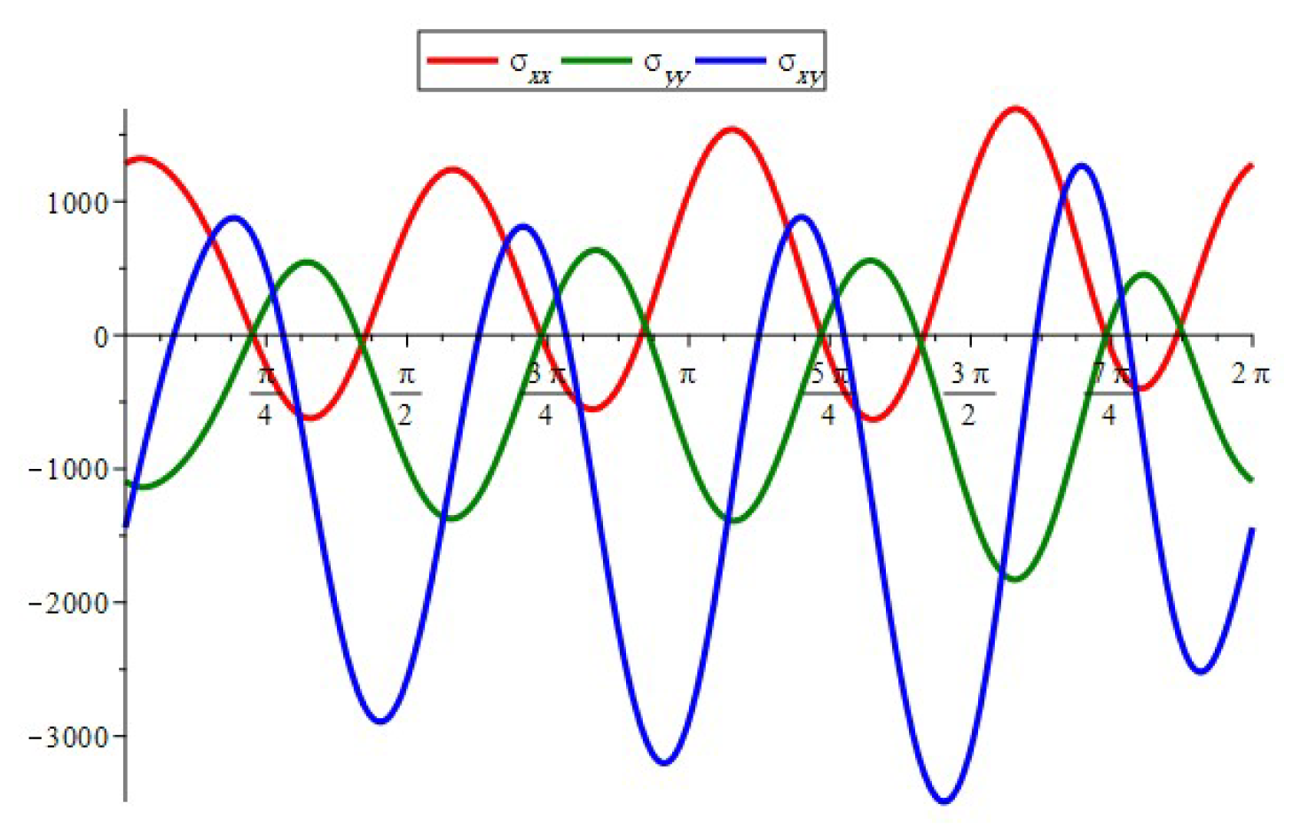
Figure 24.
Stress ratio where .
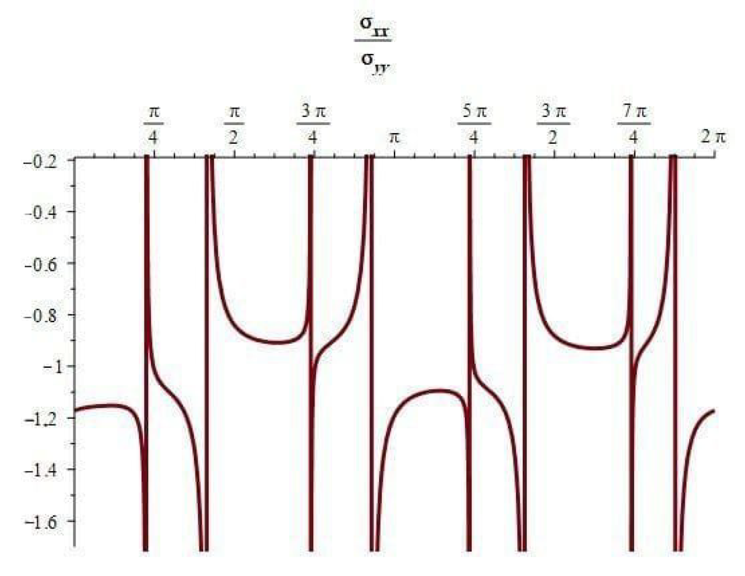
Figure 25.
Stress ratio where .
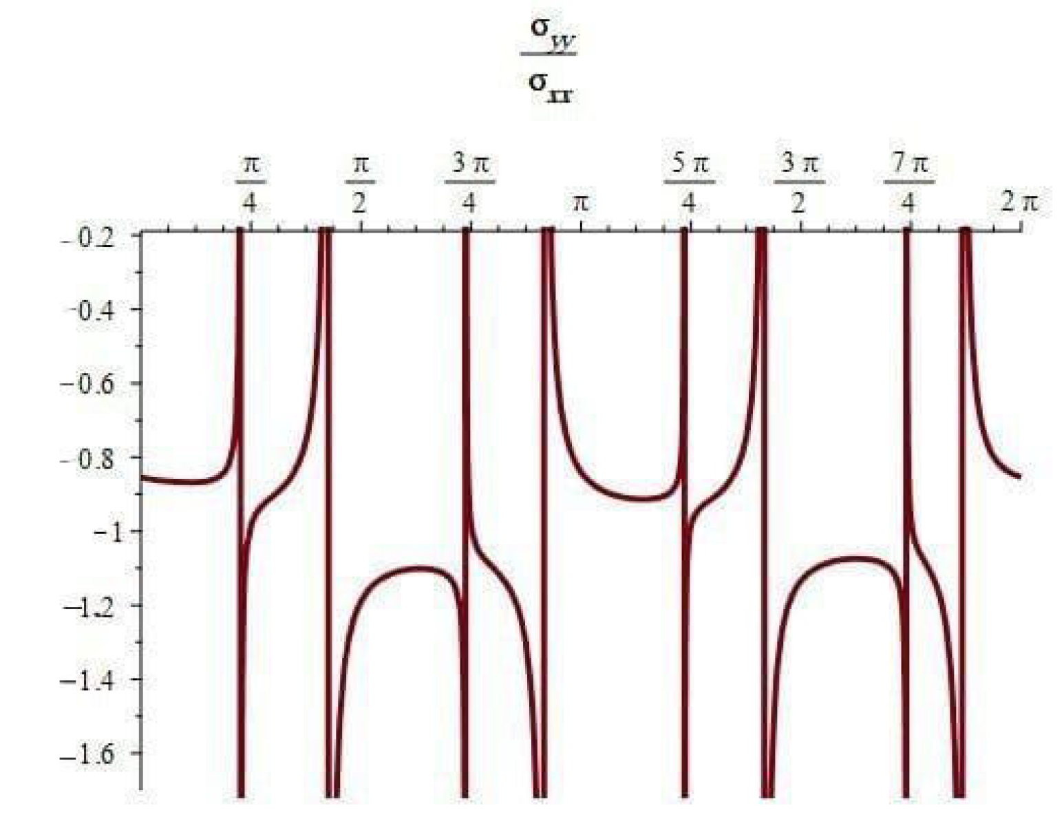
Figure 26.
The relation between stress components and the angle .

Figure 27.
Stress ratio where .
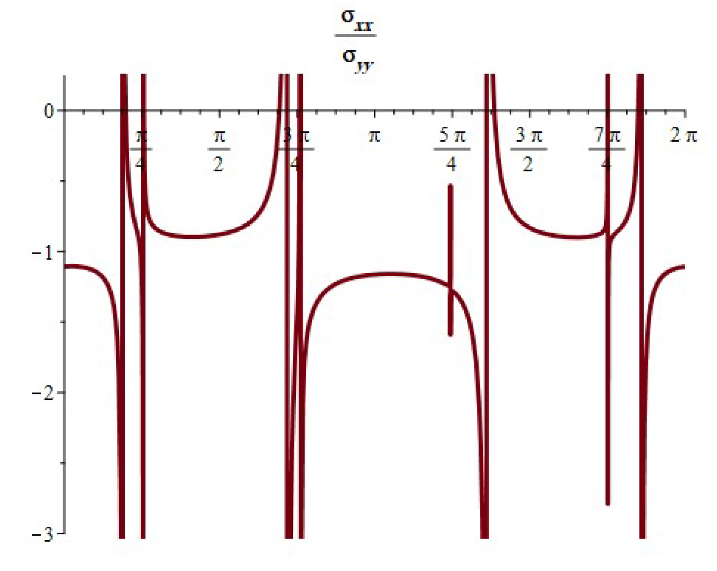
Figure 28.
Stress ratio where .
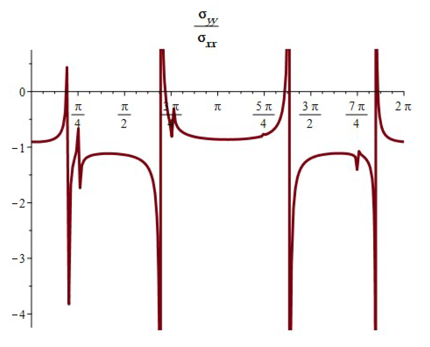
Figure 29.
The relation between stress components and the angle .
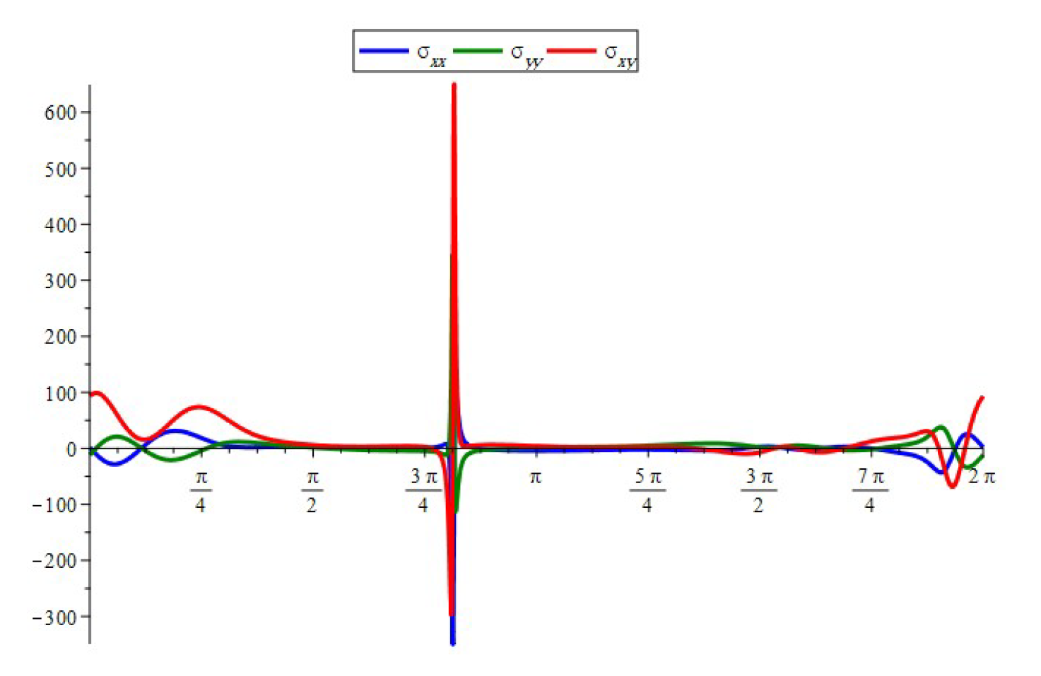
Figure 30.
Stress ratio where .

Figure 31.
Stress ratio where .
Disclaimer/Publisher’s Note: The statements, opinions and data contained in all publications are solely those of the individual author(s) and contributor(s) and not of MDPI and/or the editor(s). MDPI and/or the editor(s) disclaim responsibility for any injury to people or property resulting from any ideas, methods, instructions or products referred to in the content. |
© 2024 by the authors. Licensee MDPI, Basel, Switzerland. This article is an open access article distributed under the terms and conditions of the Creative Commons Attribution (CC BY) license (https://creativecommons.org/licenses/by/4.0/).
Share and Cite
MDPI and ACS Style
Alharbi, F.M.; Alhendi, N.G. New Approach of Normal and Shear Stress Components for Multiple Curvilinear Holes Which Weakened a Flexible Plate. Symmetry 2024, 16, 360. https://doi.org/10.3390/sym16030360
AMA Style
Alharbi FM, Alhendi NG. New Approach of Normal and Shear Stress Components for Multiple Curvilinear Holes Which Weakened a Flexible Plate. Symmetry. 2024; 16(3):360. https://doi.org/10.3390/sym16030360
Chicago/Turabian StyleAlharbi, Faizah M., and Nafeesa G. Alhendi. 2024. "New Approach of Normal and Shear Stress Components for Multiple Curvilinear Holes Which Weakened a Flexible Plate" Symmetry 16, no. 3: 360. https://doi.org/10.3390/sym16030360
Note that from the first issue of 2016, this journal uses article numbers instead of page numbers. See further details here.