
Mathematical Modeling of Robotic Locomotion Systems
by
 , , , , and
Erik Prada
1,* ,
,
Ľubica Miková
1,
Ivan Virgala
1 ,
,
Michal Kelemen
1,
Peter Ján Sinčák
1 and
and
Roman Mykhailyshyn
2
1
Department of Industrial Automation and Mechatronics, Faculty of Mechanical Engineering, Technical University of Košice, Park Komenského 8, 04200 Košice, Slovakia
2
Walker Department of Mechanical Engineering, Cockrell School of Engineering, The University of Texas at Austin, Austin, TX 78712, USA
*
Author to whom correspondence should be addressed.
Symmetry 2024, 16(3), 376; https://doi.org/10.3390/sym16030376
Submission received: 31 January 2024
/
Revised: 7 March 2024
/
Accepted: 12 March 2024
/
Published: 20 March 2024
(This article belongs to the Special Issue Symmetry in the Advanced Mechanics of Systems)
Abstract
:This article deals with the presentation of an alternative approach that uses methods of geometric mechanics, which allow one to see into the geometrical structure of the equations and can be useful not only for modeling but also during the design of symmetrical locomotion systems and their control and motion planning. These methods are based on extracting the symmetries of Lie groups from the locomotion system in order to simplify the resulting equations. In the second section, the special two-dimensional Euclidean group and its splitting into right and left actions are derived. The physical interpretation of the local group and spatial velocities is investigated, and by virtue of the fact that both of these velocities represent the same velocity from a physical point of view, the dependence between them can be found by means of the adjoint action. The third section is devoted to the modeling and analysis of the planar locomotion of the symmetrical serpentine robot; the positions and local group velocities of its links are derived, the vector fields for the local connections are given, and the trajectories of the individual variables in the lateral movement of the kinematic snake are shown. At the end of the article, the overall benefits of the scientific study are summarized, as is the comparison of the results from the simulation phase, while the most significant novelty compared to alternative publications in the field can be considered the realization of this study with a description of the relevant methodology at a detailed level; that is, the locomotion results confirm the suitability of the use of geometric mechanics for these symmetrical locomotion systems with nonholonomic constraints.
1. Introduction
Modeling biologically inspired symmetric mechanisms in mobile robotics is relatively problematic. The reason is the complexity of such mechanisms and the overall complexity of systems at multiple levels. Primary modeling of symmetric locomotion systems, where the movement or structural solution is characterized by symmetry, brings new challenges, such as the reduction of the overall dimension of the mechanism, generation of optimal gait functions, analysis of stability due to external perturbations, and identification of parameters representing appropriate biological patterns and is partly related to the overall biorealism of a complex solution. In the future, however, there will be important challenges regarding the overall energy efficiency or the adaptability of the mechanism to the changing environment and to the overall conditions affecting locomotion. In the past, several methods were developed for the description of mechanical systems, but the overall complexity of the mechanical system prevented the simple use of conventional methods. Currently, quite a lot of interest is devoted to the applications of geometric mechanics in robotics, while it has a high ability to describe a given mechanical system in a more elegant way, taking into account its geometric parameters, which can show a symmetrical character.
If we look in more detail at the concept of symmetry in combination with a mechanical solution, we can define the concept of a symmetrical mechanical system. This type of system is characterized by its geometry and design. This means that the overall mechanical system acquires a symmetrical character, which means that it is structurally symmetrical. At the same time, a part of this system is the symmetrical structure of the subsystem layout, which is mechanically balanced at the level of force action and overall structural stress.
Geometric mechanics has been used in scientific practice for decades. Its origin dates back to the sixties and seventies, when Vladimir Arnold (1966) [1], Stephen Smale (1970) [2], and Jean-Marie Souriau (1970) [3], laid the foundations of this discipline. Currently, geometric mechanics is used in a wide range of scientific fields, such as computer graphics, control theory, magnetohydrodynamics, and nonlinear stability. It is also used in the design of mechanisms for environments with active flow, such as aircraft systems, submarines, and the like. The motivation for its use in locomotion systems was probably due to the good results it achieved in solving the problems of positioning satellite systems in orbit, a falling cat, parking a car, and others. With a more detailed focus on robotic locomotion systems, we can encounter the application of geometric mechanics in several scientific works. For example, during the 1990s, in the work titled “Symmetry, Stability, Geometric Phases, and Mechanical Integrators—Part I” Marsden et al. (1991) [4], the authors presented the development of modern methods of mathematical analysis and their use for describing dynamics and overall progress in mechanics. In the work titled “Geometric Phases and Robotic Locomotion”, Kelly and Murray (1995) [5] deal with specific robotic applications, where they describe the mechanisms of a two-wheeled robot, an inchworm robot, a serpentine robot with sidewinding motion, and a six-legged robot with a tripod gait application. In the mentioned work, the authors developed and applied the theory of principal fiber bundles and the theory of connections. Geometric mechanics itself could be defined in several ways, but for our application, the most suitable definition is that geometric mechanics is a field of mechanics that deals with the study of the movement and iteration of bodies based on geometric and, at the same time, algebraic methods, with the aim of overall analysis of locomotion trajectories and identification of configuration parameters within defined spaces while using the language of differential geometry for formal description.
A more detailed view of the theory of geometric mechanics can also be obtained from the older works of Chaplygin (1897), Cartan (1928), Kobayashi and Nomizu (1963), Neimark and Fufaev (1972), Rosenberg (1977), Weber (1986), Bloch and Crouch (1992), Yang, Krishnaprasad, and Dayawansa (1993), and others. The work titled “Nonholonomic Mechanical Systems with Symmetry” by Bloch, Marsden, Krishnaprasad, and Murray (1995) [6] is considered another important work in the field. In this work, the authors deal with the development of the dynamics of mechanical systems with non-holonomic constraints, taking into account the geometric principle. This work is considered one of the basic sources for the study of the given issue. As an example, it shows the suitability of using the given approach In robotic locomotion for the entire class of possible solutions, such as legged robots, snake-like robots, and wheeled mobile robots. Within movement modeling, the theory of connection on a principal bundle is applied. An important part is the geometric phase, which generates a specific form of robot movement. Another application can be seen in the work titled “Nonholonomic Mechanics and Locomotion: The Snakeboard Example” by Ostrowski et al. (1994) [7]. The writers of this work concentrate on the design and description of the snake board-type mechanism for a better understanding of the undulating locomotion of snakes. Snake board has no biological counterpart and is an artificial imitation of the desired mechanism performing a snake-like symmetrical movement.
Important works at the beginning of the millennium include the work titled “Nonholonomic mechanics” by Bloch (2003) [8], which discusses nonholonomic mechanical systems and their control, and the work titled “Optimal Gait Selection for Nonholonomic Locomotion Systems” by Ostrowski et al. (2000) [9]. This work concentrates on the optimum control and selection of gaits in a category of nonholonomic locomotion systems that demonstrate group symmetry. Other works include, for example, A Framework for Steering Dynamic Robotic Locomotion Systems by McIsaac and Ostrowski (2003) [10], where the authors address the challenge of controlling robot motion in various dynamic environments, such as uneven terrain, obstacles, or unstable conditions, and modeling, analyzing, and controlling motion in various situations. They also present successful experimental results. The next work, titled “A method for determination of optimal gaits with application to a snake-like serial-link structure” by Hicks and Ito (2005) [11] introduces a strategy for identifying the most efficient gaits for serpentine robotic systems. The authors use optimization and simulation algorithms to identify the best walking parameters and confirm the success of the proposed method through simulation results. In the work titled “Geometric motion planning analysis for two classes of underactuated mechanical systems” by Shammas, Choset, and Rizzi (2007) [12], the authors develop gaits for two different types of underactuated mechanical systems: primarily kinematic and purely mechanical systems. They define inputs as gaits, which are a series of regulated shape changes in a multi-bodied mechanical system. A similarly important work is the article called Geometric motion planning: The local connection, Stokes’ theorem, and the importance of coordinate choice by Hatton and Choset (2011) [13], where the authors introduce two tools for understanding the fundamental principles of movement: connection vector fields and connection height functions. Connection vector fields depict the geometric link between internal shape changes and the resulting body velocities of a system.
The last decade in the field of application of geometric mechanics in the description of biologically inspired locomotion systems was also rich in interesting works and solutions. For example, the work titled “Locomotive reduction for snake robots” by Xiao et al. (2015) [14] introduces locomotive reduction, a simplifying approach that simplifies the control of a redundant snake robot to that of maneuvering a differential-drive vehicle. The next work titled “Geometric motion planning for systems with toroidal and cylindrical shape spaces” by Gong et al. (2018) [15] focuses on understanding the topology of the form space and develops geometric tools for systems with toroidal and cylindrical shape spaces. In the work titled “A hierarchical geometric framework to design locomotive gaits for highly articulated robots” by Chong et al. (2019) [16], the authors implement a hierarchic framework that decomposes a high-dimensional system into subsystems; they primarily focus on the movement of mechanical systems in two dimensions, in pairs, to achieve the desired movement of the robot. Similarly, in the work titled “Geometric phase predicts locomotion performance in undulating living systems across scales” by Rieser et al. (2019) [17], the authors focus on the geometric framework and the overall simplification of the calculations of the movement of biologically inspired robotic systems without limbs in different scales. The authors conclude that undulating locomotion in a damp environment can be applied to small organisms in viscous substances and animals navigating in viscous liquids like sand. It is therefore easy to describe the dynamics of these systems through sinusoidal modes. In the article titled “Guided Motion Planning for Snake-like Robots Based on Geometry Mechanics and HJB Equation” by Guo et al. (2018) [18], a method is proposed, through which the movement planning of a snake-like robot is realized, which is based on the re-composition of the multi-dimensional configuration space into low-dimensional fiber bundle topological space and gait space. The work thus derives a kinematic connection that maps the movement very well. In the work titled “Moving sidewinding forward: optimizing contact patterns for limbless robots via geometric mechanics” by Chong et al. (2021) [19], the authors deal with contact planning and the subsequent design of a framework for the design and optimization of contact patterns for generating efficient locomotion in the desired directions. The work is based on previous works in the field of geometric mechanics and introduces the optimization of the function that connects the contact state space and the position space. Another important work is “Coordinating tiny limbs and long bodies: Geometric mechanics of lizard terrestrial swimming” by Chong et al. (2022) [20], where the authors use the theory of geometric mechanics and its possibilities to explain observations in biological experiments. In this work, it was found that movement using body undulation with an advancing wave refers to the situation when this wave is generated by the whole body and not from the limbs (in the case of a static wave), and therefore, lizards living in the soil move in the “terrestrial swimming” manner defined by the authors. The interaction between the body and the environment during movement plays a crucial role.
Within our service robotics and mechatronics laboratory, geometric modeling techniques are used. Since 2014, our team has been evaluating and researching the geometric mechanics-based locomotion principles of biologically inspired robotic systems. As shown by several publications on the subject, we concentrate on locomotion based on body shape changes utilizing gradual cyclic waves as well as locomotion of articulated systems where a change in the limb position is applied in accordance with a predetermined movement function [21,22,23].
The suitability of the use of a geometric framework thus consists of its application in solving the problems of mobile robotics, in which the solution of mechanical problems is left to classical mechanics. It is especially suitable for use in locomotion situations with cyclic symmetric movement functions. In the following section, we will introduce basic concepts from the field of geometric mechanics that must be understood for the correct interpretation of mathematical notation. In geometric mechanics, there are many mathematical terms that represent, in most cases, abstract forms. The part itself is the description of appropriate basic forms using a special mathematical formalism. It expresses their mutual relations and subsequently, more complex constructions.
The geometric mechanics method allows one to see into the geometric structure of the equations and is used in the design, modeling, and control of motion planning. It can be used on a variety of locomotion systems, whether they are wheeled robots, legged robots, or underwater robots. It provides a deeper insight into the overall behavior of the system. Advances in the use of geometric mechanics have enabled more realistic models to be created, simulated, and then analyzed in a realistic environment.
Therefore, the aim of this study is to create a conceptual summary of the method of solving mobile non-holonomic symmetric robotic mechanisms, such as a snake-like robot, and to verify the suitability of using geometric mechanics.
2. Materials and Methods
The configuration of a symmetrical mechanical system is a set of variables q1, q2, …, qn that uniquely specify the position of any point on the mechanical system in two-dimensional or three-dimensional Euclidean space. These variables are called configuration variables or generalized variables and are characterized by the fact that they uniquely define the configuration of the mechanical system, while their n is equal to the number of degrees of freedom of the mechanical system. In a simplified way, we can write that the configuration space defines a set of possible arrangements of configurations q in the previously unbounded space known to us. In this way, we can uniquely define every single point in the configuration space that is related to the described mechanical system during its movement. The specific definition also refers to the number of degrees of freedom as they allow us to achieve a specific type of movement, such as translational, rotational, and bending. We denote the configuration space by . Its dimension is similar to the number of degrees of freedom of the mechanical system. The dimension, also known as the system dimension, represents the possibilities of movement in mechanical systems and is analogous to the dimensions in Euclidean space. We can also use generalized coordinates within this analogy.
In geometric mechanics, the configuration space of mechanical systems is also called a manifold and is geometrically most often represented by a curve, a circle, or a spherical surface. In order to have a better idea when dealing with the term manifold later, we will rigorously define it in the following subsection.
2.1. Definition of Manifold
The idea of manifold is one of the most fundamental concepts in modern mathematics, cropping up in almost all aspects of mathematics (especially geometry and topology), many parts of physics, and even some parts of engineering. Basically, manifolds are just a way to extend the idea of “surface” to more than three dimensions. Any curve that can be drawn by hand is a one-dimensional manifold, a surface such as a sphere, disc, or torus is a two-dimensional manifold, and the entire 3D space is an example of a three-dimensional manifold.
Variable P, put simply, the manifold of dimension n, is a set of points that is locally similar to the Euclidean space , that is, it is a continuous space that is locally Cartesian, and it is possible to perform differentiation on it. A manifold is therefore not a set of rational numbers. However, the rigorous definition of manifold says that the manifold is a set for which every point P lies in some open set , which is continuously uniquely mapped onto an open subset . The symbolic notation of this expression is as follows:
Within this manifold definition, is a coordinate representation, is a map, and n is the manifold’s dimension. However, the mentioned representation introduces a local coordinate system on the set , which is the inverse image of the Cartesian system or:
The entire manifold represents a complete set, usable for the given purpose of the application; for this reason, the entire manifold is covered by an atlas or a set of maps. However, local map overlays are required to be smooth enough, as shown in Figure 1.
The manifold is graphically illustrated on the example of a terrestrial globe, where the surface of the globe is an example of a simple manifold. From a geometric point of view, it is a sphere, i.e., a two-dimensional curved continuous surface, on which we can locally introduce specific maps of coordinates for individual regions. Together, the maps form an atlas that covers the entire surface of the globe. The advantage is that trajectories, as well as speeds and accelerations, can be studied on local maps. This means that derivative and integration operations can be performed locally. A manifold is therefore a space that looks like a piece of n-dimensional Cartesian space around each point. One piece of such an n-dimensional space around the selected point is called a map or local coordinates.
Each point x on this map clearly corresponds to n real numbers, i.e., its coordinates. Thanks to this, differential and integral calculus can be meaningfully developed on it. A manifold is a natural generalization of . Locally, it is the same as , but globally, it need not be. An n-dimensional manifold can be understood as being glued together from several pieces of , i.e., maps that make up an atlas. Mechanical systems, with the exception of pathological cases, “live” on manifolds.
2.2. Fundamental Configuration Blocks and Operations within the Configuration Space
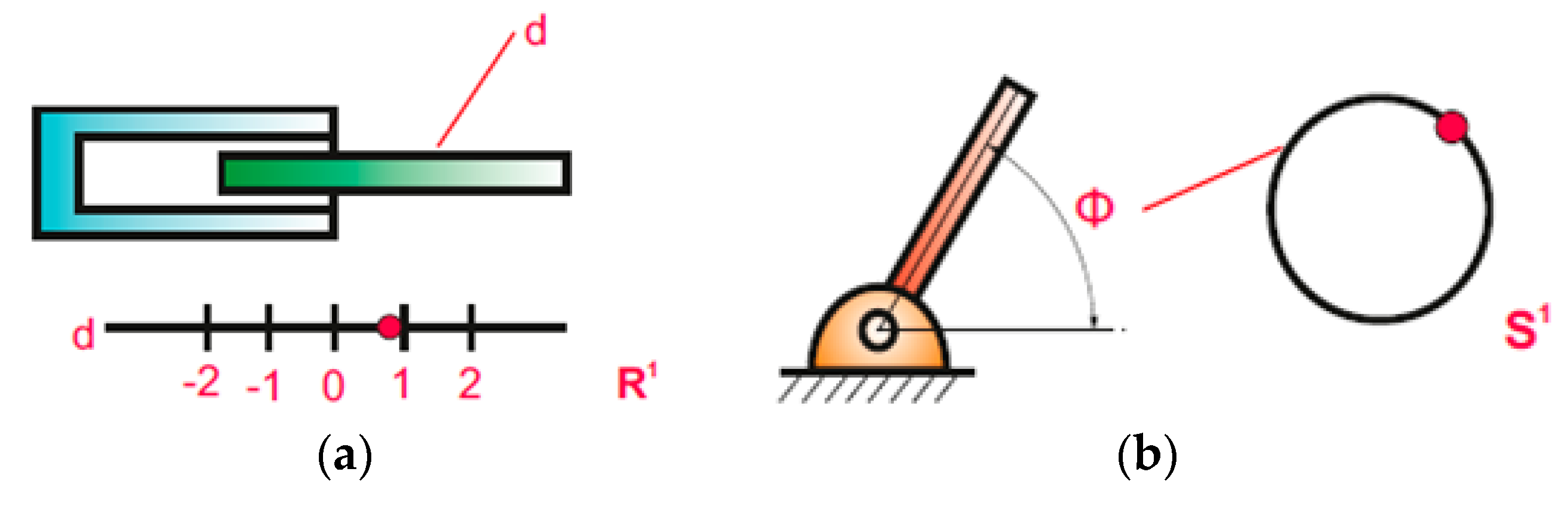
The first fundamental configuration blocks that are applicable within the design description include a straight line and a curve. In their cases, the configuration space has one dimension. Mechanically, a straight line can be expressed using a prismatic joint, and in the case of a curve, it is possible to use a tracking ball whose movement along the curve is limited. The symbolic notation makes it possible to designate such one-dimensional systems whose elements are real numbers. The second fundamental configuration block belongs to the circle denoted by the symbolic notation . In terms of application, it is represented by a cyclic movement. The set is represented by a spherical surface with one dimension. Structurally, such a block can be expressed by a wheel, a joint, or a closed loop. In these applications, a rotating circular space occurs, which is repeated cyclically. The main feature for identifying the configuration block labeled is the space’s cyclicity, Figure 2. This means that this type of block can also include a system that does not physically have a circular shape but only has a cyclical course. For this reason, this category does not include mechanical joint systems that cannot fully rotate cyclically, i.e., their ability to rotate is only partial.
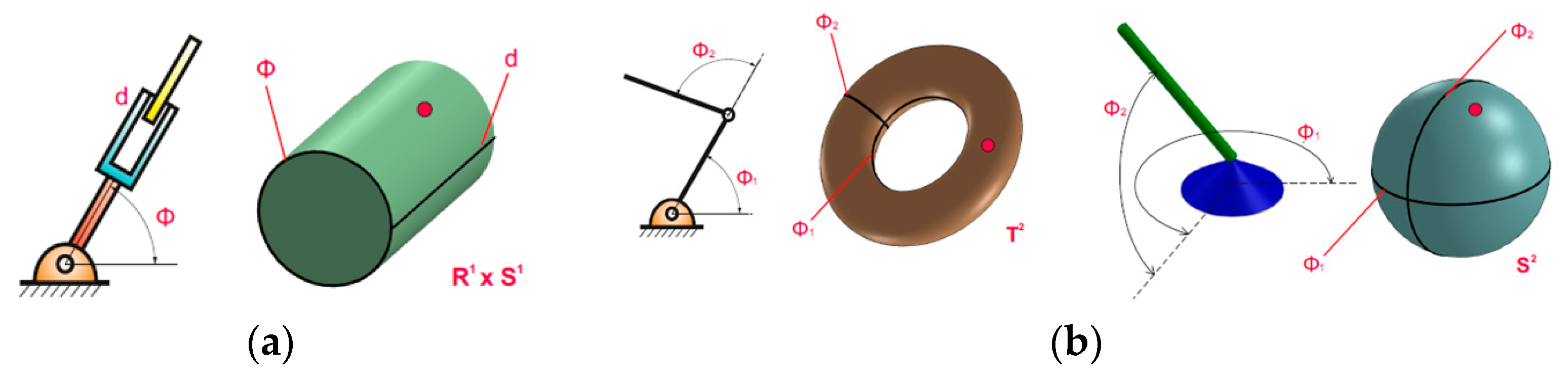
Another configuration block can be created by combining a straight line and a circular configuration block. This gives us an extended configuration block that enables the use of configuration spaces for much more complex mechanical systems. The simplest of these systems is the configuration block represented by a plane. This configuration block was created by applying the Cartesian product of two configuration blocks represented by lines. In reality, it can be a surface on which a mobile robot moves or a connection with a pair of prismatic joints. Similarly, as in the previous case, by applying the Cartesian product to two configuration blocks , which are represented by a line and a circle, we obtain a configuration block geometrically corresponding to the shape of a cylinder. Mechanically, such a block is represented by a combination of a prismatic and a rotary joint. By combining two configuration blocks in the shape of a circle, one obtains an extended configuration block , geometrically represented by a torus. In the mechanical application, it is a pair of rotary cyclic joints, as shown in Figure 3.
2.3. Lie Groups
In general, groups are important algebraic systems within mathematics. Formally, they have a good application, for example, in the description of symmetries. The group can be rigorously defined as an algebraic system with a binary operation on the set , where is a neutral element of this binary operation. The associativity condition must also be fulfilled for the binary operation :
Furthermore, it must be true that for every element , there is an inverse element with respect to the operation . If the binary operation on the given group is additionally commutative,
we call such a group an Abelian group.
However, if we operate on the set using the binary operations of addition, multiplication, or composition of functions, the notation of such algebraic systems has the following form: for addition, for multiplication, and for the composition of functions. Within algebraic systems, it is also possible to perform the so-called null operations. To clarify, for example, addition and multiplication are binary operations, and the numbers 0 and 1 are null operations on the set , where 0 is the additive identity, while 1 is the multiplicative identity. Analogously, we can write that we have a set , which we call a group if a group operation is defined as one that assigns exactly one element to each ordered pair of . It therefore applies to group :
For an algebraic system to be a group, the following conditions must be fulfilled:
- Associativity for the binary operation
- The existence of a neutral (unit) element for the operation if and only if:
- The existence of an inverse element for every :
In our case, we are mainly interested in algebraic systems from the point of view of geometry. For this specific view, there is a special class of groups called Lie groups. These are objects in which two different aspects, algebraic and geometric, coexist at the same time. In the main sense, they are groups, but they are also smooth varieties at the same time. If the group elements were not formed by a discrete set but by a continuum, it would be possible to introduce points, i.e., their coordinates in the geometric sense of the word. In calculations, there are often situations where we need to perform algebraic operations such as addition and multiplication within a certain configuration space while operating on a set of real numbers. We conduct these operations to determine the absolute configuration of a component positioned relative to a separate component or to identify the relative configuration of two separate components positioned based on an absolute expression. For example, a Lie group with an additive binary operation on a configuration block of one dimension, namely a line, has a symbolic notation of the form . Another example is the special orthogonal group , which is a rotation group in an -dimensional space. If the space has two dimensions, the rotation is defined by matrix formal notation:
represents the rotation angle in matrix notation. This matrix is cyclic, smooth, and unique with respect to the rotation angle; so, it naturally corresponds to the definition of the manifold .
2.4. Special Euclidean Group
The group encompasses the operations of rotation and translation within its structure. The movements can be categorized as “clean,” showing no signs of irregularity. Part of the Euclidean group is the orthogonal group , which represents a rotation in the planar-plane within the entire algebraic-structure. The resulting shape can be expressed as a semi-direct product of the orthogonal two-dimensional group and the planar configuration space , showcasing the interaction between rotational and translational components of the mechanism. For planar systems, the elements of the Euclidean group have four possible interpretations:
- The first interpretation refers to the position of the rigid body and its orientation at the same time.
- The second interpretation refers to the position of the coordinate frame.
- The third interpretation concerns the movement actions of both the rigid body and the coordinate frame.
- The fourth interpretation refers to the action of identifying a point in another coordinate system relative to the coordinate frame.
It is necessary to state that the first two interpretations are closely related to each other as the position and orientation of rigid bodies are essentially identified by local coordinate systems aligned with the longitudinal and transverse axes of individual links. So, for both of these interpretations, we can say that the group describes all possible configurations of the body in 2-dimensional space. The third and fourth interpretations of the group are not only related to space, but also to the Lie group, which creates a certain configuration with each specific action. The geometric meaning of these operations is in the form of rotation and displacement using a homogeneous matrix, where is the displacement vector and the orthogonal group is the submatrix consisting of the first and second rows and first and second columns. The aforementioned actions are divided into right actions and left actions. We denote the left action as and the right action as , where the element acts on the element . Since the group is not commutative like, for example, Abelian groups, the right and left group actions are also not equivalent. Expressing the action in matrix form, where is the following for the elements (represents the initial configuration of the body with respect to the origin of the coordinate system) and (represents the transformation):
The realization of the left action is the multiplication of the given matrices in the specified order (the left action of the group element to the group element ).
This resulting left action matrix represents the new rigid body position configuration. The notation of this new position takes the form of a line vector, as shown in Figure 4a.
The realization of the right action of group element on element is as follows:
This resulting right action matrix represents the new rigid body position configuration. The notation of this new position takes the form of a line vector:
By using the right action, we have thus achieved the placement of the body’s local coordinate system in a new position represented by the position vector. The graphic interpretation of the action is shown in Figure 4b. For the points p of the rigid body, which are characterized by the coordinates against the moving coordinate system and if the configuration of the rigid body is , a special calculation of the action on the group is provided in the following form:
It is clear from the matrix (19) that only the positions of the points, but not the orientation, are not considered. This process of mapping from to global system coordinates is known as direct kinematics.
Using the Euclidean group to make a mathematical model of a certain mechanism is helpful because it takes into account how the rigid bodies in the mechanism are positioned in relation to each other using the group’s action. For example, the individual displacements in the group have a reference to the global coordinate framework regarding the group, and the displacements have a reference to the initial coordinate framework. If , then the result of the right and left actions of the group is the unit element of the group , i.e., the beginning of the group configuration space.
2.5. Function, Curve, and Vectors on the Manifold
For further work with the manifold structure, we will define basic concepts such as functions, curves, and vectors on the manifold, which will help better understand the interrelationships between the formal description and the physical interpretation on a rigid body. For the function on the manifold , it is true that the representation is also a situation where each point is assigned a real number . In the local coordinates of the map , the function can be represented by its coordinate definition . Working with functions on the manifold is intuitive as physical interpretation is relatively frequent. To define the curve on the manifold , it is necessary to emphasize that it is a differentiable representation . So, the parametric curve is a smooth representation of , where is an open interval. In the local map , the surroundings of the point is parameterized by the coordinates ; so, the curve is locally defined by the functions . For our practical implementation, the curve on the manifold represents the possible trajectory of the center of gravity movement, joint coordinates, joint rotation, and a number of other interpretations. Another important concept is defining a vector on a manifold. The vector at the point located on the manifold is given by the tangent to the curve located on the manifold , while the curve passes through the point . It is characteristic of the vector v that has a direction determined by the curve and a magnitude corresponding to the magnitude of the change at time . If several different curves with different parametrization pass through the point , then the set of all vectors determined by these curves is called the tangential space . For the vectors , it is true that they lie in the tangential space , which is a linear space and not on the manifold . The application of these vectors is, for example, in the description of kinematic quantities of speed. Dealing with the speeds of the mechanical system is an essential part of the overall analysis of the behavior of the mechanism. The configuration of the body thus changes not only on the basis of the position coordinate , but also on the basis of the velocity coordinate .
2.6. Velocities of the Mechanical Systems and Tangent Spaces
When focusing on the analysis of a symmetric mechanical system, it is important to focus not only on the current position coordinates but also on their first derivatives representing the velocity coordinates . Their change simultaneously changes the overall configuration of the investigated mechanism, which actually defines its current state. After choosing a suitable configuration space for the mechanical system, the next step in modeling its behavior is determining the velocities, i.e., the speed and direction in which the mechanical system moves. In general, velocities can be interpreted geometrically as tangent vectors to the configuration of the system, corresponding to infinitesimal changes in the configuration over time. With regard to geometric mechanics, velocity vectors are elements of tangential space, which can be imagined as a tangent plane to a specific manifold. If we focus on the concept of space, we will find that it is closely connected to the definition of its dimension; that is, it depends on the dimension of the manifold. The difference is that if we consider the manifold , then, the geometric representation of such a configuration space is in the shape of a circle. In this case, the velocity vector on this manifold is geometrically represented by a tangent to the circle. The tangent space thus has one dimension. If we work with a manifold with a higher number of dimensions, such as the torus , then, in this case, the velocity vector is located in the tangential space, which is represented by the contact plane. The set of all such n-dimensional tangent spaces is a new configuration space, i.e., a new manifold, which, however, is called a tangent manifold “tangent bundle” . If we understand the configuration of the coordinate system as a point on the manifold , then its velocity is the direction, and the speed with which this point moves through the manifold is the vector that we can think of as “connected” to the manifold in the current configuration. The velocity vectors that a mechanical system can have at a given configuration are parts of a vector space named the tangent space at in that configuration, , which generally contains all possible differential changes in configuration from point . Tangent spaces on an n-dimensional manifold are vector spaces and can be conceptualized of as “linearization” of the manifold or vector spaces that come closest to the manifold at each point. The term “tangent space” reflects the idea that small changes in configuration are always in the direction contained on the manifold and are thus “tangent lines” to it. Like manifolds, tangent spaces and the vectors they contain exist as geometric objects that are independent of any coordinates used to describe them. However, to perform calculations on these vectors, it is useful to assign a basis to the tangent space so that each vector is parameterized by a set of real numbers. In the case of Rn varieties, the velocity calculation is simpler. Rigorously, we can characterize the tangent bundle as the union of all tangent spaces at all points on the manifold , that is, . Each point on the new manifold represents a specific tangent vector . For a tangent bundle, there exists a point , which determines the vector and a point , where the vector is tangent to the manifold . There is also a representation , while holds. Furthermore, for the tangent bundle, the point has the components of local coordinates in the form and the components of the vector have the form in the basis . For an existing point , it holds that it has natural components of coordinates in the form , while the representation is in coordinates defined simply as .
2.7. Lifted Actions with Vectors in the Tangent Manifold
During operations of addition and comparison of velocity vectors in individual tangent spaces and at the same time, in the tangent manifold, we will introduce a new type of method, the so-called “lifted actions”. These are directly associated with transformations. Similar to how the left and right actions apply to the Lie groups for the initial configuration , it is analogously true that the lifted actions also have a left and right variant. For example, on a Lie group, a left action applied to the initial configuration using a left-lifted action will allow a vector from the initial tangent space to be transformed into equivalent vectors in the final tangent space .
Similarly, for the right-lifted action:
Lifted actions can be calculated as differentials corresponding to the respective actions:
2.8. Velocities of a Rigid Body
In general, velocities can be interpreted geometrically as tangent vectors to the configuration of the system, corresponding to infinitesimal changes in the configuration over time. The special Euclidean group describes the configuration of a rigid body. As already mentioned, the speed of a mechanical system can be defined by how fast the group’s operations are performed. Let the inertial coordinate system and the local coordinate system be given, and let the motion of the rigid body be described by a trajectory on the group, i.e., , where is time. In a group statement, this can be expressed as:
where it is assumed that the curve is differentiable.
The velocities on Lie groups are defined by the velocity with which the infinitesimal actions of the group are applied to the configuration. Let the group (body) move by infinitesimal time :
Then the group velocity is calculated as the difference between and the unit element of the group , which is divided by the time for which the displacement was performed:
If there is a difference between the left and right actions of the group , then the relation is the right shift from to and then:
defines the right group velocity .
Substituting the left displacement into Equation (29) produces the left group velocity :
The group velocities and are an element of the tangent space in the unit group e, which is called the Lie algebra. This vector space is a linearization of a group around its unit in a very similar way as a tangent space is a linearization of a manifold around a given point. The natural basis can thus be obtained from members of the 1st order of the Taylor expansion of the group , which means that the group element representing the infinitesimal displacement is as follows:
The generation of the basis for the group velocities thus results from adjusting Equation (34) after substituting into Equation (29), removing the group unit and dividing the remainder by :
The resulting matrix in Appendix A represents an element of the Lie algebra. Its three parameters , , and describe the group velocity of a planar rigid body in the group unit. Further, the left group velocity will be called the spatial group velocity and will be denoted by the symbol , , and the right group velocity will be called the local group velocity , i.e., , and their expression will be the following:
Considering that the movement of a rigid body imitating the movement of a biological model is studied and is not acted upon by any external forces, the spatial and local velocities are constant during the movement. This results in two matrix differential equations: one with spatial and the other with local velocity.
To obtain the solution of Equation (38), assuming that , , are scalars, we will proceed with the following relations. We obtain and modify the differential equation of the first order, where the initial condition is .
Matrix equations also have analogous solutions of Equations (40) and (39):
The set of all these solutions to the differential equation for all possible initial conditions is called the flow of the vector field. We can interpret these solutions as a representation that any point moves along the integral curve from the point to the point . Formally, we can express it as and . The trajectories induced by the vector field’s flow are called integral curves (i.e., curves that do not leave the unit group at time ). Only one integral curve starts from the point , and it is called a one-parameter subgroup. The manifold of the group is thus filled with an infinite system of curves , while these curves do not intersect anywhere, and the velocity of movement along them is determined by the group velocity ξ, which is constant. The integral curve , which starts from the unit of the group , is called a one-parameter subgroup of the group . Its entire course is fully determined by where and how quickly it leaves the unit of group at time , i.e., by its tangent vector in the unit group e. Its solution has the following form:
The overall expression in and coordinates can be found in Appendix B. The final form of these equations is as follows:
From Equations (45) and (47), it is possible to notice that it is actually a representation of the group velocities , and in the Lie algebra to the configurations (positions) , and on the Lie group. This representation is called the exponential representation and is defined as:
The image of the element on the one-parameter subgroup is assigned a point to which we arrive at time if at time , we start from point with the initial velocity and for the entire time we go uniformly in a straight-line geodetics, as shown in Figure 5.
2.9. Left- and Right-Lifted Actions
It is characteristic of the left-lifted action that it preserves the expression of the velocity of the rigid body regarding the local coordinate system, the velocity of which is expressed in two different approaches. One possible way is to describe the velocity of the body in the plane using a forward, rotational, or lateral component. For the right-lifted action , in turn, it is true that it preserves the expression of the spatial velocity and its simplification of the calculation at fixed points relative to the rigid body.
The rigid body is moved from the g configuration to the center of the inertial coordinate system by the left lift action. Velocity vectors on a group are said to be equivalent if their configuration velocities are equal to the configuration velocity of the group velocity or . The use of this fact will make it possible to find the relationship between the vectors on the group and consequently, the lifted action. Let the group velocity and the velocity vector be in the configuration . Applying the left action to the configuration leads to the new configuration . The velocity vector in this configuration is denoted as . It is necessary to find the relationship (lifted action) between the velocity vector and the velocity vector . By comparing the group velocities from both configurations, we obtain the following:
The dependence between velocities , , a can be expressed in the following way:
In matrix form, the relationship between velocities is expressed as:
or by symbolic notation:
Any left action that rotates the local coordinate system by an angle accompanies the lifted action by rotating the velocity vector by the same value. In addition, the left-lifted action has an interesting property where is equal to . By combining and , a solid body is taken from and placed at the origin of the coordinate system with an equivalent velocity, thus aligning the local coordinate frame with the global frame. For the velocity of such a body:
After inverting relation (65), we can obtain the world velocities:
For the right-lifted action , in turn, it is true that it preserves the expression of the spatial velocity and its simplification of the calculation at fixed points relative to the rigid body. Just as the left-lifted action was obtained, it is also possible to determine the right-lifted action on the group . Let the group velocity and the velocity vector be in the configuration . Applying the right action to the configuration leads to the new configuration . The velocity vector in this configuration is denoted as . It is necessary to find the relationship (lifted action) between the velocity vector and the velocity vector . By comparing the group velocities of both configurations, we obtain the following:
For searched vector , a is valid:
The resulting relationship of the right-lifted action by components is as follows:
In matrix form, the relationship between velocities is expressed as:
The right-lifted action preserves the spatial velocity . This group velocity is the velocity of an imaginary point of a rigid body, which, at a given moment, passes through the beginning of the inertial coordinate system, and its value is calculated according to the following equation:
By inverting the equation, the spatial velocity becomes the world velocity for any local rigid body coordinate system:
2.10. Spatial Velocity and Its Determination Using Adjoint Operators
After applying the right action to the Euclidean group , the local coordinate system is located in the position and orientation of the group element with respect to the group element . When determining such a local coordinate system, for example, regarding articulated systems, it is subsequently appropriate to determine its velocity as a function of the group element . This speed can also be expressed using standard kinematic equations:
We can also express this velocity using the right-lifted action as follows:
As shown above, Equations (82) and (84) are the same. However, the difference is that by using the right-lifted action, its spatial velocity is preserved. The spatial velocity can be defined as the velocity of a rigid body of an imaginary point located on the rigid body at the moment it passes through the origin of the coordinate system. It is represented in the body’s local coordinate system, and we can calculate it using the following equation:
If we perform the inversion of Equation (85) by simple processing, we arrive at a relation that expresses the world speed for any local coordinate system, as follows:
The spatial velocity of a body is a suitable mathematical construction connected together with the world velocity and the velocity of the body. Adjoint operators are used for transformations between the spatial velocity and the body’s own velocity and vice versa.
These adjoint operators consist of a pair of lifted actions, and together, they can form adjoint actions of Lie groups. For example, the adjoint operation is used to map the body velocity to the spatial velocity :
The inverse adjoint operation is used for the inverse mapping of the spatial velocity to the body velocity :
The velocity vector in configuration g has the same value in the relations and . By comparing these two relationships, we obtain the following:
Their mutual dependence is obtained, as follows:
After subsequent modifications implemented in Appendix C, we obtained the final shape of the individual components of the vector :
The same applies to the inverse relationship.
where the entire form is detailed in Appendix C.
An adjoint operation is described by the following equation:
The adjoint action on the Euclidean group maps the velocity of the rigid body into the spatial velocity of the rigid body:
Similarly, the inverse adjoint action on the Euclidean group has the effect of mapping the spatial velocity of the rigid body to the velocity of the rigid body :
3. Results
This section will be devoted to the modeling and analysis of the planar locomotion of a symmetric serpentine robot with lateral shear constraints provided by passive wheels. The snake robot, which is composed of three links, performs lateral movements. Its undulating locomotion movement will be ensured by changing the size of the angles , while it has fixed wheel axles perpendicular to the body, as shown in Figure 6. The kinematic snake’s location in the plane is denoted by the variables and its configuration space is as follows:
The chosen kinematic snake has three degrees of freedom given by and the two shape variables .
3.1. Calculation of the Position of the Coordinate Systems of the Symmetric Three-Link Kinematic Snake
The coordinate systems will be marked on the simplified diagram of the kinematic snake in Figure 7, and the position calculation will be carried out from the middle link, in which the local coordinate system for the entire system with the origin in is determined, the shape of which is as follows:
In order to be able to calculate the individual positions of the first and third link, first, the position of the end of the second link h2 with respect to is calculated by moving it in the direction of the x-axis to the right by a distance L/2:
The resulting position of the end of the first link is as follows:
We calculate the position at the other end of the second link in the same way as , but by moving it to the left in the direction of the axis L/2:
The resulting position of the end of the second link is as follows:
In the case of a multi-link serpentine robot, the same procedure would, of course, be followed, while the obtained expressions for the positions of the coordinate systems become more complex with each additional member added. The key point is that the configurations of any members can be readily represented as a sequence of relative positions of the coordinate systems that result in these expressions, as shown in Figure 7.
3.2. Calculation of Local Velocities of a Three-Link Kinematic Snake
When modeling these systems, it is important to consider the functional relationship between the local velocity of each member in the kinematic chain and the total local velocity , and its shape velocity is sought. This dependence on the three-member system is investigated. The local coordinate system for the entire system is fixed to the middle member with the origin at . This choice of the local coordinate system of the system gives a trivial Jacobian at the point :
This will ensure the calculation of the velocity of other members of the chain. In order to determine the local velocity of snake body member 1, the local velocity of the end of snake body member 2 must first be found and used to calculate the local velocity of the nearer end of snake body member 1, which has a rotational speed with respect to :
Finally, the local velocity in is calculated as:
Similarly, when the local velocity of snake body member 3 is calculated, first, the local velocity of the other end of snake body member 2 is calculated, and then, it is transformed into the local velocity of the nearer end of snake body member 3. The local velocity of the other end of snake body member 2 is equal to:
It applies to local velocities , and and is adjusted to the Jacobian form:
For the three-link kinematic snake, three non-holonomic constraints are obtained without sideslip of the wheels. The individual y components of the Jacobians are expressed in the Pfaffian form:
By modifying the previous equation, the resulting relationship between the positional and shape variables of the kinematic snake is obtained, as follows:
3.3. Depiction of Local Connections Using Vector Fields
The local connection of the three-link kinematic snake is displayed using vector fields. In addition to displaying the individual components of the local connection, the vector fields also contain a generated gait ϕ, which represents the association between the shape variables, i.e., the rotations of the snake’s joints. Gait, which generates the lateral movement of the snake robot Figure 8, has the following form:
The rotation speed of the joints is obtained by differentiating the rotation angles with respect to time, Figure 9:
After defining the gait, the curve can be displayed in individual vector fields. Figure 10, Figure 11 and Figure 12 show how the kinematic snake will move in the direction of the x, y, and θ axes. If the arrows of the vector field are in the opposite direction of the sense of the generated gait, then the kinematic snake will move in the negative direction, and in the opposite case, the snake will move in the positive direction. Arrows that land perpendicular to the gait curve only cause the snake to turn. The vector field of the local connection is a zero-vector field, which results from the conditions of non-holonomy. In the case of the arrows of the local connection vector field which are parallel to the gait curve, they only cause the snake’s joints to rotate, and the snake does not rotate in the direction perpendicular to the curve.
4. Conclusions
Based on the results from Section 3.3, where the simulation results were presented, we can conclude that when applying the serpentine lateral movement to the symmetrical kinematic snake, the individual vector fields, together with the drawn movement curves, give us information about the real behavior in individual sections of the movement. Individual sections of the curve are represented by points 1, 2, 3, 4, and 5. The key input in this case is the shape of the function ϕ. The gradual shape change of the robotic snake’s body is realized by simultaneously setting the rotation angles and in the snake’s joints. The results show a simplified diagram of the layout of individual links and their sizes and angles in the joints of the model. The current gradual change of rotation in time is interpreted in the output results figures. The green color identifies the total cycle of change of rotation of both angles, which corresponds to a time of 6.5 s for both angles simultaneously. Similarly, for the angular speeds of rotation of the joints, in the result figure, we can see the cyclic character of the change in the angular speeds and . When comparing these shape parameters, it is clear that the magnitude of the speed in the initial phases of the movement is greater. At the same time, however, it is necessary to take into account the influence of non-holonomic restrictions on the movement of the snake, which will be manifested by the impossibility of direct movement in the perpendicular direction at the location of the individual wheels.
The total movement of the robot globally expresses the vector field of the connection in the direction of the x and y axes and the angle θ. Is presented in the results the vector field together with the gait curve, on which the positions of the points within one cycle are highlighted in black. It is the position of the points on the gait curve and the influence of the vectors at the location of the given point that represent the overall character of the symmetrical movement. The effect of the non-holonomic constraint can be seen in results too, where no vector field acts in the corresponding plane during the cycle of the gait curve. For a proper understanding, the overall rotation of the central link at the center of gravity, i.e., the overall orientation of the entire body of the snake and its gradual change during one cycle of the curve.
A three-link robotic snake with non-holonomic constraints, which has two action quantities of rotation changes and at the joints, moves in a lateral cyclic motion, while the changes of the shape of the body based on the change of the shape variables are equal to the respective phases of the movement in points 1 to 5, Figure 13. Finally, we can observe the change in the coordinates of the global variables x, y, and angle during the simulation verification. It can be seen in Figure 14 that the movement of turning the angle is repeated cyclically. Movement in the y-axis direction is forbidden precisely because of non-holonomic constraints. For this reason, the value Y of the transformation is equal to the constant 0.
The most important research findings can be summarized in the following points:
- To implement the locomotion of a three-link snake robot of the under-actuated type, the shape of the robot is changed in order to achieve the required movement function through the rotation of the joints.
- During the locomotion of the mechanism, there is also a cyclical change of an-gular velocities when it is found that the velocities are greater in the initial phases of the movement.
- From the results of the simulation of a three-link snake robot during the cyclic phases of locomotion, it follows that visualizing the local connection through a vector field clearly contributes to the body shape changes. Moreover, it is related to the overall control of the mechanism and depends on the input geometric parameters.
- The equation of the input movement curve is an important influencing parameter for the overall resulting shape of the movement of the mechanism.
Based on these findings, we can conclude that when modeling a mobile robotic mechanism with non-holonomic constraints, we must pay attention not only to non-holonomic constraints but also to the classification of shape variables, the shape of motion functions, and the overall geometric symmetry of the mechanism. Based on this, we can, to a certain extent, generalize the use of the given method to multi-element systems with non-holonomic constraints.
The advantages of using a geometric approach to describe the principle of locomotion of a biologically inspired snake robot are clearly visible in the graphic representation and in the simplification of the mathematical description of the symmetric mechanical system. Geometric mechanics provides a mathematical framework for accurately describing the motion and kinematic properties of a robot. Using geometric tools such as Lie groups and algebras, it is possible to mathematically model and analyze the movement of a robot in space, and it is also possible to analyze the movement of different types of robots, regardless of their specific construction and mechanical parameters. In addition, it allows for optimizing the design of the robot’s movement and searching for efficient trajectories. Using the principles of differential geometry and variation, it is possible to evaluate the energy requirements, stability, and other properties of the robot’s movement. All this makes geometric mechanics a powerful tool for describing locomotion and its physical understanding.
Author Contributions
Conceptualization, E.P. and Ľ.M.; formal analysis, Ľ.M. and E.P.; funding acquisition, M.K. and I.V.; methodology, Ľ.M.; software, E.P.; formal analysis, I.V.; investigation, M.K. and R.M.; resources, Ľ.M. and P.J.S.; data curation, E.P. and P.J.S.; writing—original draft preparation, E.P.; writing—review and editing, E.P.; visualization, Ľ.M.; supervision, M.K.; project administration, I.V. and R.M. All authors have read and agreed to the published version of the manuscript.
Funding
This research was funded by the Slovak Grant Agency VEGA 1/0201/21 Mobile mechatronic assistant, Slovak Grant Agency VEGA 1/0436/22 research on modeling methods and control algorithms of kinematically redundant mechanisms, and the Cultural and Educational Grant Agency of the Ministry of Education, Science, Research and Sports of the Slovak Republic KEGA 027TUKE-4/2022 Implementation of Internet of Things technology to support the pedagogical process in order to improve the specific skills of graduates of the study program of industrial mechatronics.
Data Availability Statement
Data are contained within the article.
Conflicts of Interest
The authors declare no conflicts of interest.
Appendix A
An illustrative example of the calculation of the first two terms of of the Taylor series is:
By substituting Equation (A2) into Equation (29) and after a small modification, we obtain the following:
After the adjustments, the matrix shape is as follows:
Appendix B
Based on Equation (44), we express the position of the object in coordinates and as follows:
Appendix C
By substituting the respective matrices into the individual members and performing matrix operations, the resulting relationship based on Equation (90) is obtained, as follows:
where
Appendix D
Position of the first link:
where represents the transition from one link to the next by rotating by an angle :
after substituting into the following equation:
Next, the more distant remaining positions of the first link are determined, as follows:
The positions of the coordinate systems for the third link are derived in the same way:
The local velocity of the nearer end of link 1 will have the following form:
We calculate the local velocity by moving L/2 in the direction of the x-axis to the right:
When deriving the local velocities of the third link, the same procedure will be followed:
References
- Arnold, V. Sur la géométrie différentielle des groupes de Lie de dimension infinie et ses applications à l’hydrodynamique des fluides parfaits. Ann. L’institut Fourier 1966, 16, 319–361. [Google Scholar] [CrossRef]
- Smale, S. Topology and mechanics. I. Invent. Math. 1970, 10, 305–331. [Google Scholar] [CrossRef]
- Souriau, J.-M. Structure des Systèmes Dynamiques: Maîtrises de Mathématiques; Dunod: Paris, France, 1970; ISBN 2-04-010752-5. (In French) [Google Scholar]
- Marsden, J.E.; O’Reilly, O.M.; Wicklin, F.J.; Zombro, B.W. Symmetry, stability, geometric phases, and mechanical integrators. Nonlinear Sci. Today 1991, 1, 4–11. [Google Scholar]
- Kelly, S.D.; Murray, R.M. Geometric phases and robotic locomotion. J. Robot. Syst. 1995, 12, 417–431. [Google Scholar] [CrossRef]
- Bloch, A.M.; Krishnaprasad, P.S.; Marsden, J.E.; Murray, R.M. Nonholonomic mechanical systems with symmetry. Arch. Ration. Mech. Anal. 1996, 136, 21–99. [Google Scholar] [CrossRef]
- Ostrowski, J.; Lewis, A.; Murray, R.; Burdick, J. Nonholonomic mechanics and locomotion: The snakeboard example. In Proceedings of the 1994 IEEE International Conference on Robotics and Automation, San Diego, CA, USA, 8–13 May 1994; pp. 2391–2397. [Google Scholar]
- Bloch, A.M. Nonholonomic Mechanics; Springer: New York, NY, USA, 2003. [Google Scholar]
- Ostrowski, J.P.; Desai, J.P.; Kumar, V. Optimal gait selection for nonholonomic locomotion systems. Int. J. Robot. Res. 2000, 19, 225–237. [Google Scholar] [CrossRef]
- McIsaac, K.A.; Ostrowski, J.P. A framework for steering dynamic robotic locomotion systems. Int. J. Robot. Res. 2003, 22, 83–97. [Google Scholar] [CrossRef]
- Hicks, G.; Ito, K. A method for determination of optimal gaits with application to a snake-like serial-link structure. IEEE Trans. Autom. Control 2005, 50, 1291–1306. [Google Scholar] [CrossRef]
- Shammas, E.A.; Choset, H.; Rizzi, A.A. Geometric motion planning analysis for two classes of underactuated mechanical systems. Int. J. Robot. Res. 2007, 26, 1043–1073. [Google Scholar] [CrossRef]
- Hatton, R.L.; Choset, H. Geometric motion planning: The local connection, Stokes’ theorem, and the importance of coordinate choice. Int. J. Robot. Res. 2011, 30, 988–1014. [Google Scholar] [CrossRef]
- Xiao, X.; Cappo, E.; Zhen, W.; Dai, J.; Sun, K.; Gong, C.; Travers, M.J.; Choset, H. Locomotive reduction for snake robots. In Proceedings of the 2015 IEEE International Conference on Robotics and Automation (ICRA), Seattle, WA, USA, 26–30 May 2015; pp. 3735–3740. [Google Scholar]
- Gong, C.; Ren, Z.; Whitman, J.; Grover, J.; Chong, B.; Choset, H. Geometric motion planning for systems with toroidal and cylindrical shape spaces. In Proceedings of the Dynamic Systems and Control Conference, Atlanta, GA, USA, 30 September–3 October 2018; p. V003T32A013. [Google Scholar]
- Zhong, B.; Ozkan-Aydin, Y.; Sartoretti, G.; Rieser, J.; Gong, C.; Xing, H.; Choset, H.; Goldman, D. A hierarchical geometric framework to design locomotive gaits for highly articulated robots. In Proceedings of the Robotics: Science and Systems, Virtual, 22–26 June 2019. [Google Scholar]
- Rieser, J.M.; Chong, B.; Gong, C.; Astley, H.C.; Schiebel, P.E.; Diaz, K.; Pierce, C.; Lu, H.; Hatton, R.L.; Choset, H.; et al. Geometric phase predicts locomotion performance in undulating living systems across scales. arXiv 2019, arXiv:1906.11374. [Google Scholar]
- Guo, X.; Zhu, W.; Fang, Y. Guided motion planning for snake-like robots based on geometry mechanics and HJB equation. IEEE Trans. Ind. Electron. 2018, 66, 7120–7130. [Google Scholar] [CrossRef]
- Chong, B.; Wang, T.; Lin, B.; Li, S.; Choset, H.; Blekherman, G.; Goldman, D. Moving sidewinding forward: Optimizing contact patterns for limbless robots via geometric mechanics. In Proceedings of the Robotics: Science and Systems, Virtual, 12–16 July 2021. [Google Scholar] [CrossRef]
- Chong, B.; Wang, T.; Erickson, E.; Bergmann, P.J.; Goldman, D.I. Coordinating tiny limbs and long bodies: Geometric mechanics of lizard terrestrial swimming. Proc. Natl. Acad. Sci. USA 2022, 119, e2118456119. [Google Scholar] [CrossRef]
- Miková, L.; Gmiterko, A.; Kelemen, M.; Virgala, I.; Prada, E.; Hroncová, D.; Varga, M. Motion control of nonholonomic robots at low speed. Int. J. Adv. Robot. Syst. 2020, 17, 1729881420902554. [Google Scholar] [CrossRef]
- Lipták, T.; Gmiterko, A.; Kelemen, M.; Virgala, I.; Prada, E.; Menda, F. The use of geometric mechanics concept at kinematic modeling in mobile robotics. Procedia Eng. 2014, 96, 273–280. [Google Scholar] [CrossRef]
- Prada, E.; Kelemen, M.; Gmiterko, A.; Virgala, I.; Mikova, L.; Hroncova, D.; Varga, M.; Sincak, P.J. Locomotive, principally kinematic system of snakelike robot mathematical model with variable segment length. In Proceedings of the 2020 19th International Conference on Mechatronics-Mechatronika (ME), Prague, Czech Republic, 2–4 December 2020; pp. 1–6. [Google Scholar]
Figure 1.
Imagination of manifold with a local map and its representation into .

Figure 2.
A physical representation of the configuration space of a type (a) and (b).

Figure 3.
A physical representation of the configuration space: (a) and (b) and .

Figure 4.
Representation of (a): action of the Euclidean group as rotation and displacement of the object from position 1 to position 3; representation of (b): action of the Euclidean group.
Figure 4.
Representation of (a): action of the Euclidean group as rotation and displacement of the object from position 1 to position 3; representation of (b): action of the Euclidean group.

Figure 5.
Exponential representation in graphic form.

Figure 6.
A simplified diagram of a symmetric three-link kinematic snake.

Figure 7.
Designation of coordinate systems on the three-link kinematic snake.

Figure 8.
Display of rotation angles of joints and with the green line marked period for the lateral movement of the kinematic snake.
Figure 8.
Display of rotation angles of joints and with the green line marked period for the lateral movement of the kinematic snake.

Figure 9.
Display of the rotational speeds of the joints and with the green line marked period for the lateral movement of the kinematic snake.
Figure 9.
Display of the rotational speeds of the joints and with the green line marked period for the lateral movement of the kinematic snake.

Figure 10.
Vector field (blue arrows) of local connection along on cyclic gait (green line).

Figure 11.
Without vector field (no blue arrows) of local connection along on cyclic gait (green line).
Figure 11.
Without vector field (no blue arrows) of local connection along on cyclic gait (green line).

Figure 12.
Vector field (blue arrows) of local connection along on cyclic gait (green line).

Figure 13.
Lateral movement of a three-link kinematic snake with a marked trajectory of the center of gravity of the middle red link.
Figure 13.
Lateral movement of a three-link kinematic snake with a marked trajectory of the center of gravity of the middle red link.

Figure 14.
Characteristics of the dependence of the values of the x, y coordinates and the angle over time.
Figure 14.
Characteristics of the dependence of the values of the x, y coordinates and the angle over time.

Disclaimer/Publisher’s Note: The statements, opinions and data contained in all publications are solely those of the individual author(s) and contributor(s) and not of MDPI and/or the editor(s). MDPI and/or the editor(s) disclaim responsibility for any injury to people or property resulting from any ideas, methods, instructions or products referred to in the content. |
© 2024 by the authors. Licensee MDPI, Basel, Switzerland. This article is an open access article distributed under the terms and conditions of the Creative Commons Attribution (CC BY) license (https://creativecommons.org/licenses/by/4.0/).
Share and Cite
MDPI and ACS Style
Prada, E.; Miková, Ľ.; Virgala, I.; Kelemen, M.; Sinčák, P.J.; Mykhailyshyn, R. Mathematical Modeling of Robotic Locomotion Systems. Symmetry 2024, 16, 376. https://doi.org/10.3390/sym16030376
AMA Style
Prada E, Miková Ľ, Virgala I, Kelemen M, Sinčák PJ, Mykhailyshyn R. Mathematical Modeling of Robotic Locomotion Systems. Symmetry. 2024; 16(3):376. https://doi.org/10.3390/sym16030376
Chicago/Turabian StylePrada, Erik, Ľubica Miková, Ivan Virgala, Michal Kelemen, Peter Ján Sinčák, and Roman Mykhailyshyn. 2024. "Mathematical Modeling of Robotic Locomotion Systems" Symmetry 16, no. 3: 376. https://doi.org/10.3390/sym16030376
Note that from the first issue of 2016, this journal uses article numbers instead of page numbers. See further details here.