Abstract
In data analysis using a nonparametric regression approach, we are often faced with the problem of analyzing a set of data that has mixed patterns, namely, some of the data have a certain pattern and the rest of the data have a different pattern. To handle this kind of datum, we propose the use of a mixed estimator. In this study, we theoretically discuss a developed estimation method for a nonparametric regression model with two or more response variables and predictor variables, and there is a correlation between the response variables using a mixed estimator. The model is called the multiresponse multipredictor nonparametric regression (MMNR) model. The mixed estimator used for estimating the MMNR model is a mixed estimator of smoothing spline and Fourier series that is suitable for analyzing data with patterns that partly change at certain subintervals, and some others that follow a recurring pattern in a certain trend. Since in the MMNR model there is a correlation between responses, a symmetric weight matrix is involved in the estimation process of the MMNR model. To estimate the MMNR model, we apply the reproducing kernel Hilbert space (RKHS) method to penalized weighted least square (PWLS) optimization for estimating the regression function of the MMNR model, which consists of a smoothing spline component and a Fourier series component. A simulation study to show the performance of proposed method is also given. The obtained results are estimations of the smoothing spline component, Fourier series component, MMNR model, weight matrix, and consistency of estimated regression function. In conclusion, the estimation of the MMNR model using the mixed estimator is a combination of smoothing spline component and Fourier series component estimators. It depends on smoothing and oscillation parameters, and it has linear in observation and consistent properties.
1. Introduction
Often, we have to carry out statistical analyses that involve relationships between several variables in the sense of functional relationships between response variables and predictor variables. The appropriate statistical analysis to use in cases like this is regression analysis. In this regression analysis, basically, we build a mathematical model that is usually called a regression model, where the functional relationship between variables in the model is represented by a regression function, and for analysis purposes, we must estimate this regression function. In general, there are two basic types of regression model, namely, a parametric regression model and nonparametric regression model. Meanwhile, if we combine these two basic types of regression model, we will obtain a regression model called a semiparametric regression model. The parametric regression model is suitable for use in cases where the pattern of the relationship between the response variables and predictor variables is known in the sense of indicating a certain curve shape, such as linear, quadratic, cubic, etc., either through the results of initial investigations based on scatter diagrams or from past experience regarding the relationship between these variables. Hereinafter, the nonparametric regression model is suitable for use in cases where the pattern of the relationship between the response variables and predictor variables is unknown in the sense that it does not indicate the shape of a particular curve. The shape of the curve is only assumed to be smooth, that is, it is contained in a Sobolev space [1].
To estimate the regression functions of the regression models such as a parametric regression model, nonparametric regression model, and semiparametric regression model, several smoothing techniques are used, which are represented by estimators. Until now, several estimators have been discussed by several previous researchers both theoretically and in application in several cases. Some of these estimators are local linear estimators, which are used to determine the boundary correction of regression function of the nonparametric regression model [2], to determine the bias reduction in the estimating regression function [3], and to design a standard growth chart used for assessing toddlers’ nutritional status [4]; as a local polynomial estimator used to estimate regression functions in cases of errors-in-variable [5], in case of correlated errors [6], and to estimate the regression function of a functional data regression model [7] and finite population regression model [8]; as a kernel estimator used for estimating nonparametric regression function [9], for estimating and investigating the consistency property of a regression function [10], and for estimating regression function in case of correlated errors [11]. However, these estimators (i.e., local linear, local polynomial, and kernel) are less flexible because they are highly dependent on the neighborhood of the target point, called bandwidth, so that we need a small bandwidth to estimate a fluctuating data model, and this will cause a curve of estimation result that is too rough. Also, these estimators do not include penalty function as smoothness factor; these estimators only consider the goodness of fit factor. This means that these estimators are not so good for estimating models of data that fluctuate in the subintervals, because these estimators will return the estimation results with large value of mean squared errors (MSEs). On the other hand, spline estimators, especially the smoothing spline estimator, have the ability to handle these problems because the splines consider not only the goodness of fit factor but also the smoothness factor [1,12]. Further, the spline estimators such as the smoothing spline, M-type spline, truncated spline, penalized spline, least square spline, linear spline, and B-spline estimators are more flexible than other estimators to use for estimating the nonparametric regression functions, especially for prediction and interpretation purposes [12,13]. These splines have been used and developed widely in several cases by many researchers. For example, Liu et al. [14] and Gao and Shi [15] used M-type splines for analyzing the variance in correlated data, and for estimating regression functions of nonparametric and semiparametric regression models, respectively; Chamidah et al. [16] used truncated splines to estimate mean arterial pressure for prediction purposes, Chamidah et al. [17] and Lestari et al. [18] developed truncated spline and smoothing spline estimators, respectively, for estimating semiparametric regression models and determining the asymptotic properties of the estimator; Tirosh et al. [19], Irizarry [20], Adams et al. [21,22], Lee [23], and Maharani and Saputro [24] discussed smoothing spline for problems of analyzing fractal-like signals, minimizing risk estimate, modeling ARMA observations and estimating smoothing parameter, selection smoothing parameter using simulation data, and determining GCV criterion, respectively; Wang [13], Wang and Ke [25], Gu [26], and Sun et al. [27] discussed smoothing splines in ANOVA models; Wang et al. [28] applied a bivariate smoothing spline to data of cortisol and ACTH hormones; Lu et al. [29] used a penalized spline for analyzing current status data; Berry and Helwig [30] compared tuning methods for penalized splines; Islamiyati et al. [31,32] developed a least square spline for estimating two responses of nonparametric regression models and discussed linear spline in the modeling of blood sugar; and Kirkby et al. [33] estimated nonparametric density using B-Spline. Additionally, Osmani et al. [34] estimated the coefficient of a rates model using kernel and spline estimators.
In statistical modeling such as regression modeling, we often have to analyze the functional relationship between response variable and predictor variable where there are two or more response variables and the between responses are correlated with each other. The regression models that draw a functional relationship between response variables and predictor variables with correlated responses are the multiresponse nonparametric regression (MNR) model and multiresponse semiparametric regression (MSR) model. Due to there being correlation between responses, in the estimation process of a regression function, we need to include a matrix called a weight matrix. The inclusion of a weight matrix in the estimation process is what differentiates the MNR model from a uniresponse nonparametric regression (UNR) model, where there is no correlation between responses. So, the process of estimating the regression functions of the MNR and MSR models requires a symmetric weight matrix, namely, a diagonal matrix. We can also use several estimators to estimate the regression functions of these MNR and MSR models. One of these estimators is the smoothing spline estimator. Currently, many researchers are paying attention to developing and applying the smoothing spline estimator in many areas of research. For example, Chamidah et al. [17], Lestari et al. [18] discussed smoothing splines in MSR models; Lestari et al. [35] and Wang et al. [28] discussed RKHS in an MNR model and applied an MNR model to determine associations between hormones, respectively. Because of its powerful and flexible properties, the smoothing spline estimator is one of the most popular estimators used for estimating the regression functions of UNR and MNR models.
The previous description shows that the smoothing spline estimator has been used in statistical analysis using regression model approaches such as UNR and MNR models. The smoothing spline estimator provides good fitting results because it can overcome the curve of data, which has a sharp decrease and increase pattern that results a relatively smooth curve. Also, using the smoothing spline provides several advantages in that it has unique statistical properties, enables visual interpretation, can handle smooth data and functions, and can readily handle data that change at certain subintervals [1,12,13]. Meanwhile, the Fourier series estimator is a popular smoothing technique in nonparametric regression modeling. The Fourier series also provides good statistical and visual interpretation among nonparametric regression models. Using the Fourier series estimator provides advantages such as being able to handle data that have a repeating pattern at a certain trend interval and to provide good statistical interpretation [36]. Suparti et al. [37], Mardianto et al. [38], and Amato et al. [39] proposed Fourier series methods for modeling inflation in Indonesia, for modeling longitudinal data, and for approximating separable models, respectively.
The research discussed in the previous description relating to the estimation of nonparametric regression models is still limited to the use of only one type of estimator, whereas in data analysis using a nonparametric regression approach, we are often faced with the problem of analyzing a set of data that has mixed patterns, namely, some of the data have a certain pattern and the rest of the data have a different pattern. To handle these kinds of data, we should use a mixed estimator, namely, a combination of more than one estimator. Mariati et al. [40] discussed a uniresponse multivariable nonparametric regression model using a mixed estimator comprising a smoothing spline and Fourier series that was applied to data of poor households in Bali Province. However, previous researchers, namely, Mariati et al. [40], discussed the use of a mixed estimator to estimate a nonparametric regression model, but they only discussed estimating a UNR model in the sense that there is no correlation between the response variables. In this study, therefore, we theoretically discuss a new estimation method using a mixed estimator for a nonparametric regression model with two or more response variables and predictor variables, and there is a correlation between the response variables. The model is called the multiresponse multipredictor nonparametric regression (MMNR) model. The mixed estimator used for estimating the MMNR model is a combination of smoothing spline and Fourier series suitable for analyzing data wherein some patterns partly change at certain subintervals, and others follow a recurring pattern in a certain trend. Since there is a correlation between responses in the MMNR model, a weight matrix is involved in its estimation process. Also, we apply the reproducing kernel Hilbert space (RKHS) method to penalized weighted least square (PWLS) optimization for estimating the regression function of our MMNR model. In this study, therefore, we discuss theoretically about determining the smoothing spline component and Fourier series component of the MMNR model, determining the goodness of fit and penalty components of PWLS optimization, determining the MMNR model estimate, determining the weight matrix, selecting optimal smoothing and oscillation parameters in the MMNR model, and investigating the consistency of the regression function estimator of the MMNR model. Additionally, the results of this study contribute to the development of the field of theoretical statistics, namely, statistical inference theory, regarding theories of estimation and hypothesis testing in multiresponse multipredictor nonparametric regression based on a mixed smoothing spline and Fourier series estimator.
2. Materials and Methods
To achieve the objectives of this research, in this section, we briefly present materials and methods such as the MMNR model, mixed smoothing spline and Fourier series estimator, reproducing kernel Hilbert space (RKHS), and penalized weighted least square (PWLS) optimization.
2.1. The MMNR Model
We first consider a paired dataset for and . We say that the paired dataset follows an MMNR model if the relationship between and () satisfies the following functional equation:
where represents responses; represents observations; is the value of the response variable at the observation and response; is the unknown regression function of the response; are values of smoothing spline predictor variables at the observation and response; are values of Fourier series predictor variables at the observation and response; and is the random error at the observation and response, which has mean of zero and variance of . Here, we assume that the correlation between responses is .
Since the shape of the regression function in the MMNR model is assumed to be unknown and additive in nature, the regression function in Equation (1) can be presented as follows:
where ; ; is a smoothing spline component of regression function in which , are contained in a Sobolev space , namely, ; and is a Fourier series component of regression function that is approximated by a Fourier series function. Hereinafter, based on Equations (1) and (2), we have the following MMNR model:
Furthermore, the regression function of the MMNR model presented in (3) is estimated using a mixed smoothing spline and Fourier series estimator by applying the reproducing kernel Hilbert space (RKHS) method to the developed penalized weighted least square.
2.2. Mixed Smoothing Spline and Fourier Series Estimator
To estimate the regression function of the MMNR model presented in (3), we use a mixed smoothing spline and Fourier series estimator, which is suitable for analyzing data with some patterns that partly change at certain subintervals, and others that follow a recurring pattern in a certain trend. The regression function in the MMNR model in (3) consists of the component , which is approached by smoothing spline, and the component , which is approximated by the following Fourier series function:
where ; ; and .
Since we involve a smoothing spline estimator in the process of estimating the regression function, according to Wahba [12] and Wang [13], we should use the reproducing kernel Hilbert space (RKHS) method approach, which is applied to the developed penalized weighted least square (PWLS) optimization.
2.3. Reproducing Kernel Hilbert Space (RKHS)
The reproducing kernel Hilbert space (RKHS) method was first introduced by Aronszajn [41]. The RKHS method was developed for estimating nonparametric regression models and semiparametric regression models by several researchers such as Wang [13], Chamidah et al. [17], Lestari et al. [18], and Kimeldorf and Wahba [42]. We call a Hilbert space an RKHS on a set X over field if it meets certain conditions, as shown by Aronszajn [41], Berlinet and Thomas-Agnan [43], Paulsen [44], and Yuan and Cai [45]:
- (i)
- If is a vector, then , namely, is the subspace of a vector space over , which is notated by (X,);
- (ii)
- If is equipped with an inner product, , then it will be a Hilbert space;
- (iii)
- If is a linear evaluation functional that is defined by for every X, then the linear evaluation functional is bounded.
Furthermore, if , namely, is an RKHS on , then there exists a unique vector, , for every , such that for every . Note that every linear functional that is bounded will be given by the inner product with a unique vector in , and under this condition, we call the function as a reproducing kernel (RK) for the point . This means that the reproducing kernel (RK) for is a two-variable function, which is defined by . It implies that and [41,42,43,44,45].
In this study, the RKHS method is employed to the developed penalized weighted least square (PWLS) optimization for obtaining the estimation of the regression function of the MMNR model presented in (3). In the following section, we provide the penalized weighted least square (PWLS) optimization that we developed according to the case of our interest.
2.4. Penalized Weighted Least Square (PWLS) Optimization
Since the regression function of the multiresponse multipredictor nonparametric regression (MMNR) model in (3) consists of two components, namely, the smoothing spline component and the Fourier series component , for estimating the regression function, we developed the PWLS optimization for a single-estimator case, namely, the smoothing spline estimator, only as proposed by Wang et al. [28], Lestari et al. [18], and Islamiyati et al. [31], to the two mixed estimators, namely, the smoothing spline and Fourier series estimators. In the process of estimating the regression function of the multiresponse multipredictor nonparametric regression (MMNR) model by using the developed penalized weighted least square (PWLS) optimization, we assume that is a fixed function. Hence, we can estimate the smoothing spline component in the multiresponse multipredictor nonparametric regression (MMNR) model presented in (3) for every response by using the following developed penalized weighted least square (PWLS) optimization:
where ; ; ; and represents a weight that is an inverse of variances. Note that we include a weight in the developed penalized weighted least square (PWLS) presented in (5) because in this case there is a correlation between responses.
3. Results and Discussions
In this section, we theoretically discuss the estimating process of the multiresponse multipredictor nonparametric regression (MMNR) model. Firstly, suppose that we have a paired dataset such as for and , where the functional relationship between predictor variables and response variables meets the MMNR model presented in Equation (3), namely:
where information and assumptions about the multiresponse multipredictor nonparametric regression (MMNR) model are presented in Section 2.1.
Since this multiresponse multipredictor nonparametric regression (MMNR) model has more than one response variable and predictor variable, and has a regression function that is composed of two components, namely, a smoothing spline component and a Fourier series component, to simplify the process of estimating the multiresponse multipredictor nonparametric regression (MMNR) model by using the reproducing kernel Hilbert space (RKHS) method approach that is employed to the developed penalized weighted least square (PWLS) optimization, we should express the multiresponse multipredictor nonparametric regression (MMNR) model presented in Equation (3) in the form of matrix notation, as follows:
Furthermore, we may write the MMNR model presented in (6) as follows:
Hence, the MMNR model given in (7) can be written as follows:
where ; ; ;
- ; ; ;…; ; ;
- ;…; ;
- ; ;…;
- ; ;
- ; …; .
Next, by letting , we may write the MMNR model given in (8) as follows:
In the following sections, we discuss about determining smoothing spline component and Fourier series component of MMNR model, determining goodness of fit and penalty components of PWLS optimization, estimating the MMNR model, estimating the weight matrix, selecting optimal smoothing and oscillation parameters in the MMNR model, and investigating the consistency of regression function estimator of MMNR model.
3.1. Determining Smoothing Spline Component of MMNR Model
To determine the function of the smoothing spline component of the regression function of multiresponse multipredictor nonparametric regression (MMNR) model presented in Equation (1), we use the RKHS method, which is applied to PWLS optimization. Due to being a smoothing spline component in the MMNR model presented in (3), we use the RKHS method to estimate it with the following steps: Firstly, suppose that we decompose a Hilbert space into a direct sum of Hilbert subspaces with basis where represents the order of polynomial spline, with basis where represents the number of observations, and (i.e., is perpendicular to ), as follows:
Hence, we express every function where as follows:
where ; ; and are constans; ; ; ; .
Secondly, suppose is a bounded linear functional, and , then we have the following relationship:
Since is a bounded linear functional, then according to Yuan and Cai [45] and Lestari et al. [35], there exists a representer that meets the following equation:
Based on Equations (10) and (11), we may write Equation (12) as follows:
Hence, for , we may write Equation (13) as follows:
Next, based on Equation (14) for and , we have as follows:
Similarly, based on Equation (14) for and , we have as follows:
If we continue this process for and in a similar way, then for , we have as follows:
Furthermore, based on Equation (13) for , we have as follows:
Hence, based on Equation (17) for and , we have as follows:
In similar way, based on Equation (17) for and , we have as follows:
We continue this process for and in a similar way such that for we have as follows:
Based on Equations (15)–(17), we obtain the smoothing spline component of the regression function of the MMNR model for and as follows:
Next, in the same way as in the process of obtaining Equation (22), we obtain for as follows:
Since , we have matrix as follows:
Based on Equations (22) and (23), we obtain the smoothing spline component for the response, namely, , as follows:
Finally, based on Equation (25), we obtain the smoothing spline component for all responses , namely, , as follows:
where
- ;
- ;
- ;
- ;
- .
Thus, the smoothing spline component of the MMNR model can be presented in matrix notation as given in Equation (26), that is, .
3.2. Determining Fourier Series Component of MMNR Model
We consider the Fourier series component of the regression function of the MMNR model presented by Equation (3), namely, . Note that the curve shape of is unknown and only assumed to be contained in a continuous space . Based on Equation (4), this component is approximated by Fourier series function as follows:
Next, for , we may express the Fourier series function given in Equation (27) as follows:
Hence, based on Equation (28), we can write the Fourier series component of the regression function of the MMNR model for as follows:
where , , and
Furthermore, based on Equation (29) and in the same way as in the process of obtaining Equation (26), we obtain the Fourier series component for all responses , namely, , as follows:
where
- ;
- ;
- .
3.3. Determining Goodness of Fit and Penalty Components of PWLS Optimization
To estimate the regression function of the MMNR model, we use the PWLS as presented in Equation (5), namely, by taking the solution to the following PWLS optimization:
where ; ; ; and represents a weight that is an inverse of random error variances.
Based on Equations (8) and (9), we have the MMNR model, which can be expressed as or where z . Therefore, by considering Equation (26), the PWLS optimization can be written in matrix notation as follows:
where is a symmetrical weight matrix that is the inverse of a covariance matrix of random errors. Details of the weight matrix can be found in Lestari et al. [18,35]. In addition, the PWLS optimization function presented in Equation (31) shows that the goodness of fit component of PWLS optimization is .
Next, we determine the penalty component of PWLS optimization. In the PWLS optimization function presented in Equation (31), is a penalty component of PWLS optimization. In this step, we also express in matrix notation as follows:
Hence, based on Equation (32), we obtain the penalty component of PWLS optimization, which can be expressed in matrix notation for the response as follows:
Furthermore, based on Equation (33) and in the same way as in the process of obtaining Equation (26), the penalty component for all responses can be obtained as follows:
Let be the response penalty, and the penalty component for all responses is presented by as follows:
where
- ;
- ;
- .
Thus, the goodness of fit component of the PWLS optimization is presented as follows:
and the penalty component of the PWLS optimization is presented as follows:
3.4. Estimating the MMNR Model
The PWLS optimization presented in Equation (31) is used to obtain the estimation of the MMNR model. Also, we definitely consider Equations (26), (30) and (34). In this section, we provide a complete explanation of the estimation process of the MMNR model. In Equation (31), we have the PWLS as follows:
In this step, we first determine the estimator for , namely, , as follows:
Let such that Equation (35) can be written as follows:
Next, we determine the estimator for , namely, , as follows:
By substituting Equation (36) into Equation (37), we obtain the following equation:
Since , then we have , and we may therefore write Equation (38) as follows:
Equation (39) returns the following result:
By substituting Equation (40) into Equation (36), we obtain the following result:
Hence, based on Equations (26), (40) and (41), we obtain the following estimated smoothing spline component:
Thus, the estimation of the smoothing spline component of the MMNR model notated as is given by
where , and is a special symmetric weight matrix, namely, a diagonal matrix, which is an inverse of a covariance matrix of random errors. In this case, based on the assumption of random errors of the MMNR model, the weight matrix is given as follows [18,35]:
where
In the previous explanation, we obtained , which is presented in (42). The next step is determining the Fourier series component of the regression function of the MMNR model. Let us look again at the MMNR model presented in Equation (8):
We substitute Equation (42) into Equation (8) such that we obtain the following equation:
Next, we substitute Equation (30), namely, , into Equation (43) such that we obtain the equation for random error as follows:
Hence, we have
Furthermore, based on Equation (44), we determine the estimator for , namely, , as follows:
Additionally, by substituting Equation (45) into Equation (30), we obtain the estimator for the Fourier series component of the regression function of the MMNR model, namely, , as follows:
where .
Hereinafter, by substituting Equation (46) into Equation (42) we obtain the estimator for the smoothing spline component of the regression function of the MMNR model as follows:
where .
Finally, based on Equations (2), (8), (46) and (47), we obtain the estimation of the regression function of the MMNR model, which consists of estimations of the smoothing spline component and Fourier series component as follows:
Thus, the estimation result of the MMNR model by using the mixed smoothing spline and Fourier series estimator is as follows:
where λ represents the smoothing parameter of the smoothing spline estimator, represents the oscillation parameter of the Fourier series estimator,
Next, in the following section, we discuss the estimation of weight matrix W.
3.5. Estimating Weight Matrix W
Suppose that we have a paired dataset for and , which follows the MMNR model, and we assume that is a normally distributed random sample with a mean of m and covariance of such that we have a likelihood function as follows:
Since , then we may write the likelihood function as follows:
Hence, the estimated weight matrix can be obtained by determining the solution to the following optimization:
Hereinafter, according to Johnson and Wichern [46], we can determine the maximum value of each component of the likelihood function by taking the following equations:
Furthermore, based on Equation (48), we have
where . Hence, we obtain the maximum likelihood estimator for the weight matrix as follows:
where , , …, .
This shows that the estimated weight matrix obtained is a symmetric matrix, especially a diagonal matrix whose main diagonal components are the estimated weight matrices of the first response, second response, and so on, up to the R-th response.
Next, in the following section, we provide discussion on selecting optimal smoothing and oscillation parameters in the MMNR model.
3.6. Selecting Optimal Smoothing and Oscillation Parameters in the MMNR Model
In statistical analysis using an MMNR model approach based on a mixed smoothing spline and Fourier series estimator, selecting the optimal smoothing parameter and oscillation parameter, namely, (), cannot be neglected, and it is crucial to good regression function fitting of the MMNR model based on the mixed smoothing spline and Fourier series estimator. In other words, the mixed smoothing spline and Fourier series estimator highly depends on both the smoothing parameter and oscillation parameter. Therefore, in this study, we also need to discuss selecting the optimal smoothing and oscillation parameters. There are some criteria used for selecting the smoothing parameter, including minimizing CV (cross-validation), GCV (generalized cross-validation), Mallows’ , and AIC (Akaike’s information criterion) [1,12]. However, according to Ruppert and Carroll [47], for good fitting of a regression function based on a spline estimator, Mallows’ and GCV were very satisfactory.
In this study, we use the GCV criterion, which has been developed for multiresponse cases to determine the optimal smoothing parameter and oscillation parameter values for good regression function fitting of the multiresponse multipredictor nonparametric regression (MMNR) model. Firstly, we determine the mean squared errors (MSEs) of the regression function presented in (48) as follows:
where λ represents the smoothing parameter of the smoothing spline estimator, represents the oscillation parameter of the Fourier series estimator,
- ,
- , and
- .
Secondly, based on the given in Equation (49), we have the GCV (generalized cross-validation) for the MMNR model as follows:
Hence, based on the GCV function presented in (50), we can obtain the optimal smoothing parameter () and optimal oscillation parameter (K) values, namely, (), by taking the solution to the following optimization:
where represents a positive real number set. Thus, the optimal values of both smoothing parameter and oscillation parameter, namely, (), can be obtained by taking the solution to the optimization function given in Equation (51).
Furthermore, in the following section, we determine one of the statistically sound estimator properties, namely, the consistency property.
3.7. Consistency of Regression Function Estimator of MMNR Model
To investigate the consistency of the regression function estimator of the MMNR model, , firstly, we should investigate asymptotic properties of the mixed smoothing spline and Fourier series estimator, , based on an integrated mean squared error (IMSE) criterion. In this study, we develop the IMSE from the uniresponse with one predictor case proposed by Wand and Jones [48] and multiresponse with one predictor case proposed by Lestari et al. [35] into a multiresponse with multipredictor case. Next, by considering Equation (48), the IMSE can be decomposed into two components, namely, the component and component, as follows:
where , , is a weight matrix, and as given in Equation (48) is a regression function of the MMNR model.
Next, by using Theorem 2 in Lestari et al. [35], we obtain as , where represents the “big oh”. We can find the details of the “big oh” in Wand and Jones [48], and Sen and Singer [49]. Also, by using Theorem 3 in Lestari et al. [35], we obtain as and for every response . Hence, we obtain the asymptotic property of the mixed regression function estimator of the MMNR model based on the IMSE criterion as follows:
where , , , and .
Furthermore, based on Equation (53), we obtain an inequality as follows:
Hence, according to Sen and Singer [49] and Serfling [50], for any small positive number, , we obtain the following relationship:
Since then by considering Equation (54) and by applying the properties of probability, we obtain the following equation:
Equation (55) shows that the regression function estimator, , of the multiresponse multipredictor nonparametric regression (MMNR) model obtained by using the mixed smoothing spline and Fourier series estimator is a consistent estimator based on the integrated mean squared error (IMSE) criterion.
Next, in the following section, we provide a simulation study.
3.8. Simulation Study
In this section, we provide a simulation study to show the performance of the mixed smoothing spline and Fourier series estimator in estimating the MMNR model. In other words, the simulation study provided is intended to show the sensitivity of parameter selection and its impact on model performance. In this simulation study, we used generation data of with a correlation of 0.95 and a variance of 0.25. Here, we use a three-response MMNR model as follows:
Next, to show the influence of smoothing parameters (λ) and oscillation parameters (K), we use different smoothing parameters by generating lambda (λ) randomly, and different oscillation parameters by moving K from 1 to 4. We carry out this process 15 times until the optimal values of smoothing parameters (λ) and oscillation parameters (K) are obtained.
Simulation results including MSE (mean squared error) values, minimum GCV (generalized cross-validation) values, coefficient of determination () values, and lambda (λ) values for every oscillation parameter value are given in Table 1.

Table 1.
Values of MSE, minimum GCV, , and λ.
Table 1 presents the optimal lambda values based on the minimum GCV values from 15 repetitions of the MMNR model presented in Equation (56) for every oscillation parameter (K) where . From Table 1, we can observe that every different value of both the smoothing parameter and oscillation parameter will give different performance to the estimation performance. These are indicated by the different coefficient of determination () and MSE (mean squared errors) values as the values change due to oscillation parameters (K) and smoothing parameters (λ).
Next, based on all the minimum GCV values presented in Table 1, we chose the minimum GCV value from the four oscillation parameter (K) values. In Table 1, the minimum GCV value is produced by , namely, 0.5786323, with an MSE value of 1.02363794, value of 0.95311712, and ; ; . In Table 1, these values are shown in bold. These values are the optimal values and the best MMNR estimate is obtained based on these optimal values. Therefore, these values are then used to determine the estimated values of the MMNR model and to produce the plots of the estimated values of the MMNR model presented in Equation (56).
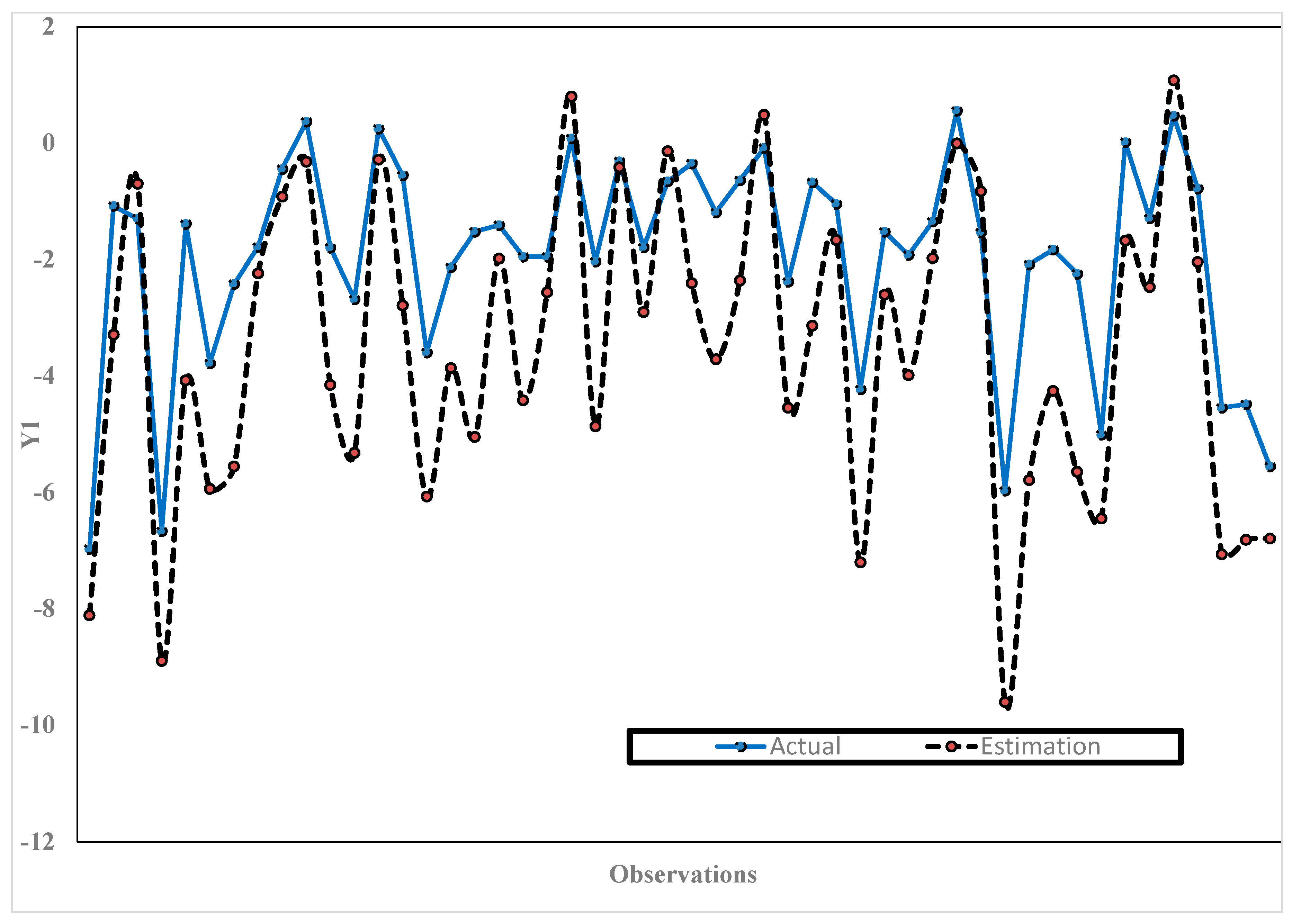
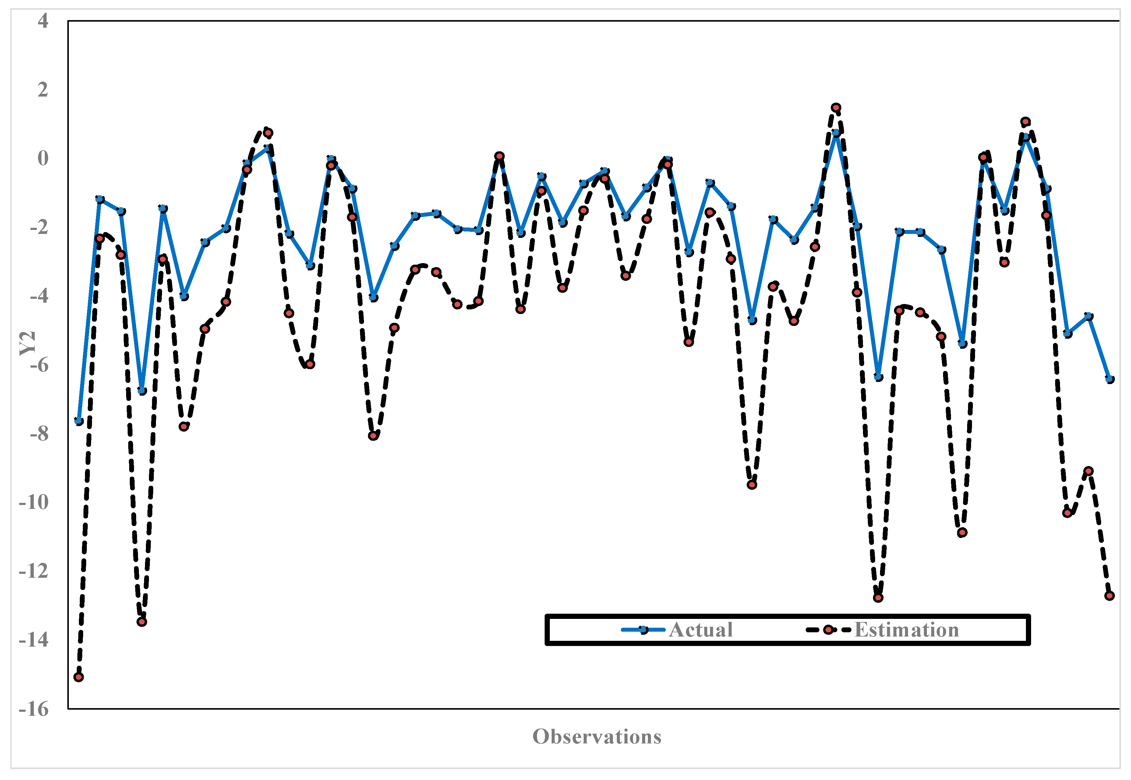
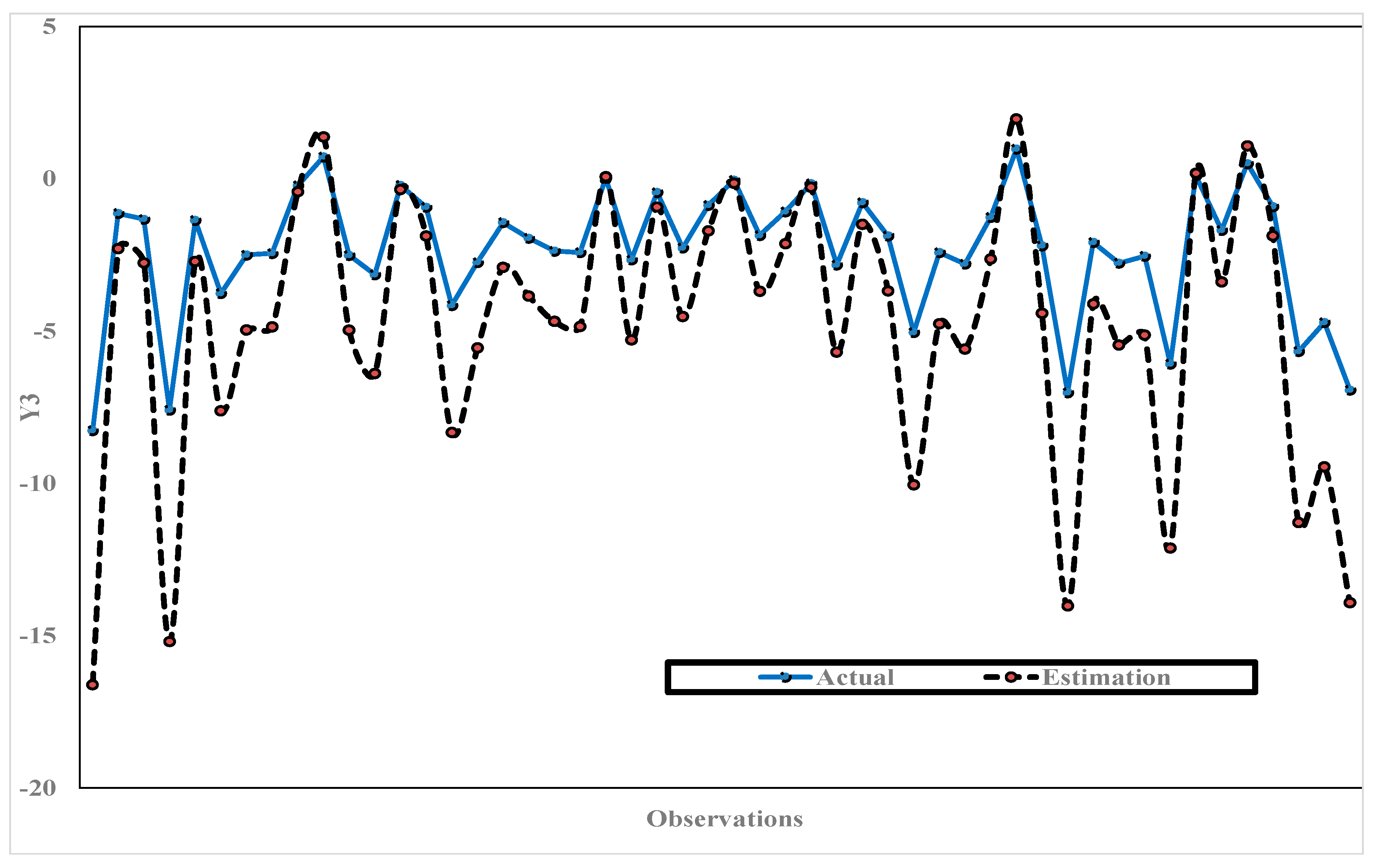
Hereinafter, we obtained the plots of estimated model values versus predictor (observation) values for every response together with the plots of their actual values. The plots of estimated model values versus predictor (observation) values for the first response together with the plots of actual values of the first response are presented in Figure 1. The plots of estimated model values versus predictor (observation) values for the second response together with the plots of actual values of the second response are presented in Figure 2. The plots of estimated model values versus predictor (observation) values for the third response together with the plots of actual values of the third response are presented in Figure 3.
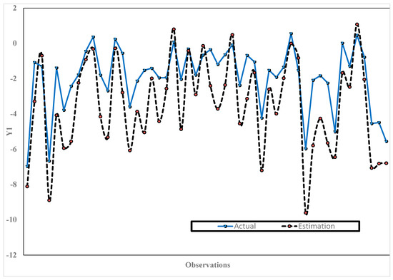
Figure 1.
Plots of estimated model values versus predictor (observation) values for the first response () together with the plots of actual values of the first response.
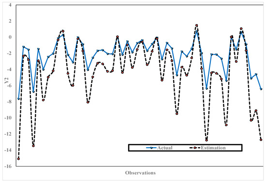
Figure 2.
Plots of estimated model values versus predictor (observation) values for the second response () together with the plots of actual values of the second response.

Figure 3.
Plots of estimated model values versus predictor (observation) values for the third response () together with the plots of actual values of the third response.
From Figure 1, Figure 2 and Figure 3, we can observe that the values of the estimated MMNR models using the mixed smoothing spline and Fourier series estimator are close to the actual values. This is shown by the performance curves of the values of the estimated MMNR models, which tend to be similar to the actual values curves. Hence, based on the results of the simulation study presented in Table 1, and Figure 1, Figure 2 and Figure 3, it shows that the estimation value of the MMNR model in (56) depends on both the smoothing spline parameter and oscillation parameter. In other words, it shows that the selection of the smoothing spline parameter and oscillation parameter is sensitive and impacts the MMNR model’s performance.
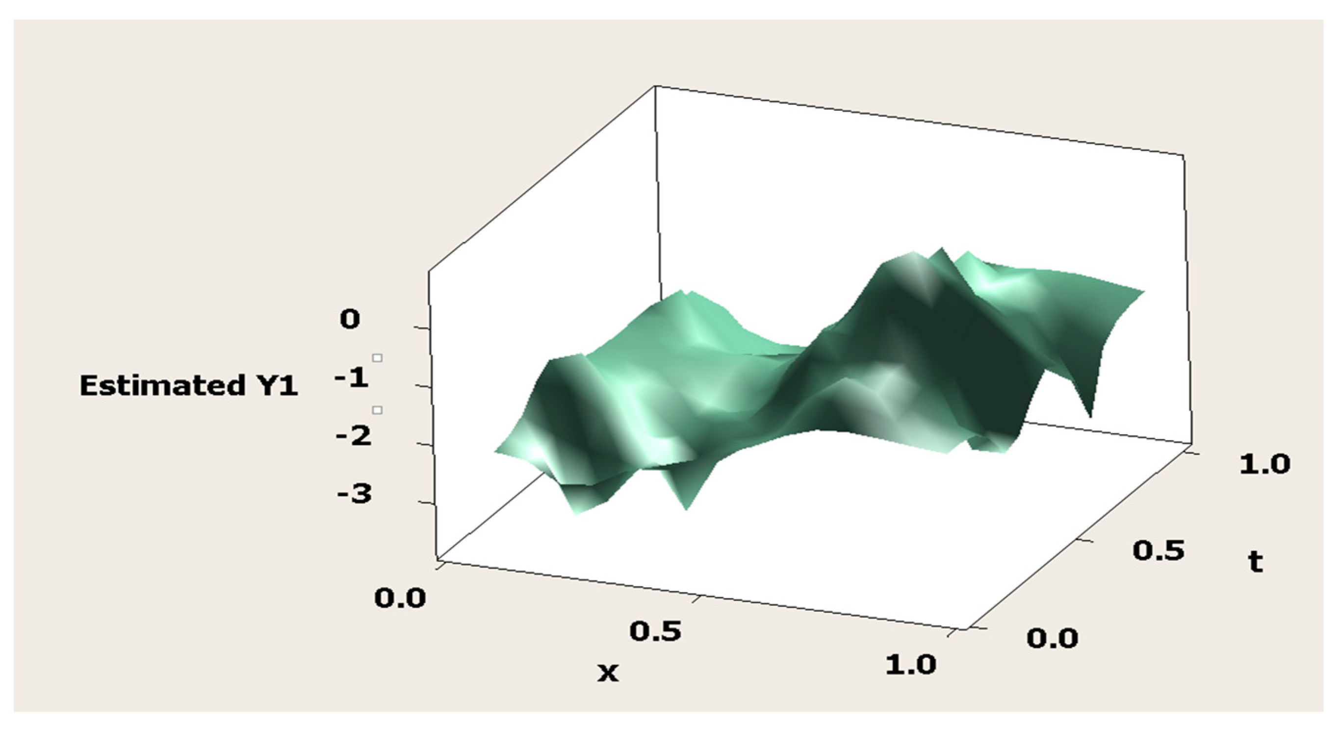
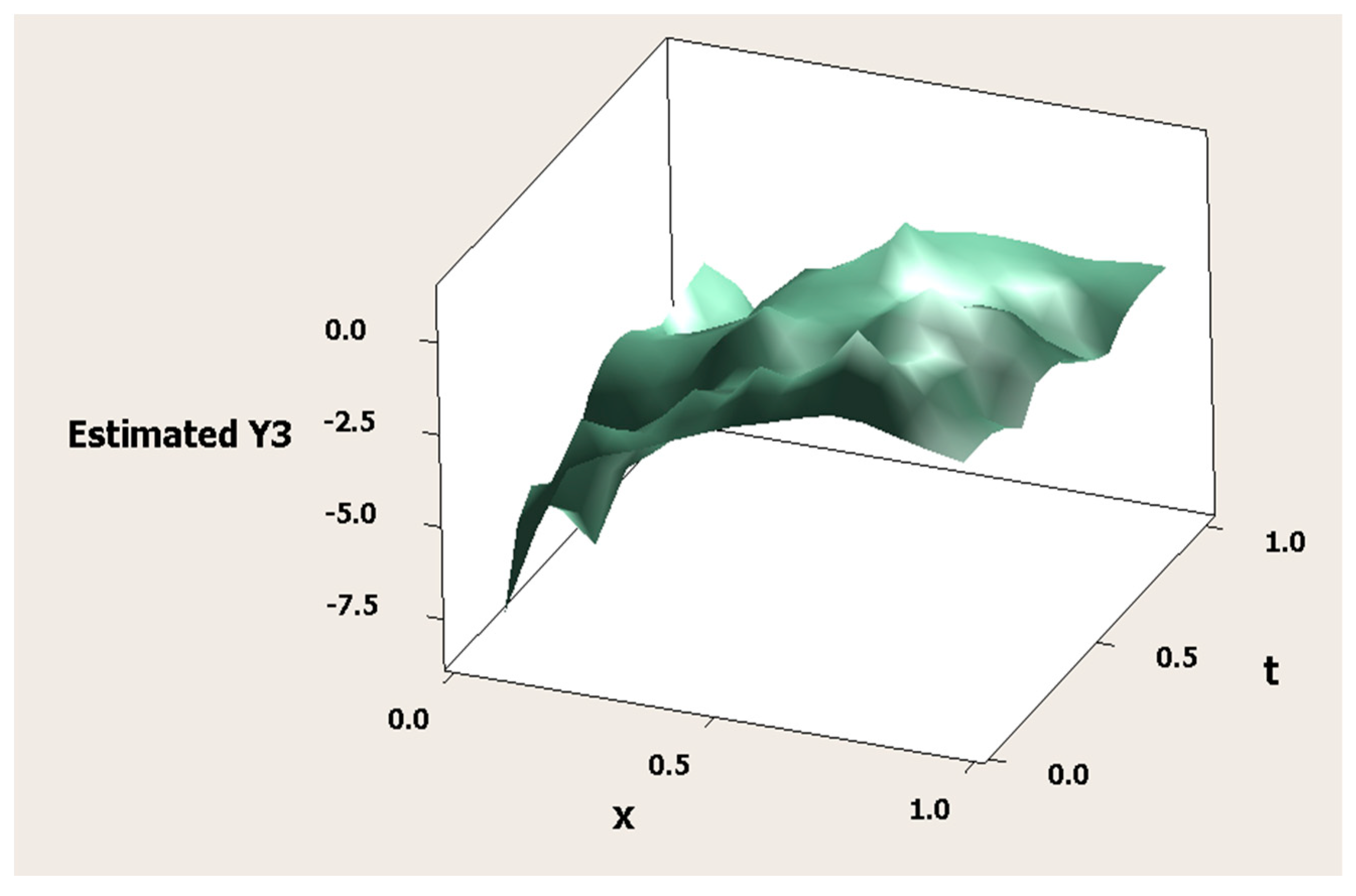
Hereinafter, based on the results of the simulation study, we obtained the surface plots of the estimation results of the MMNR model presented in Equation (56). These surface plots of the estimated MMNR model are presented in three-dimensional plots (see Figure 4, Figure 5 and Figure 6).
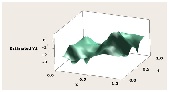
Figure 4.
Surface plot of the estimated model versus predictors for the first response ().
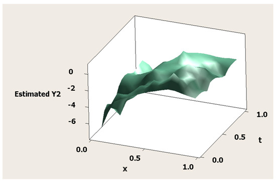
Figure 5.
Surface plot of the estimated model versus predictors for the second response ().

Figure 6.
Surface plot of the estimated model versus predictors for the third response ().
4. Conclusions
The estimation result of the MMNR model by using the mixed smoothing spline and Fourier series estimator, presented by , is a combination of the smoothing spline component and Fourier series component estimators presented by and , respectively. The estimator of the MMNR model is highly dependent on the smoothing parameter () and oscillation parameter (K). These optimal parameter values, namely, (), are determined by using the GCV criterion to determine the values that minimize the function . Also, the estimator of the MMNR model by using the mixed smoothing spline and Fourier series estimator that we have obtained is linear with respect to the observations given in Equation (48). Additionally, the regression function estimator, , of the MMNR model obtained by using the mixed smoothing spline and Fourier series estimator is a consistent estimator based on the IMSE criterion. This means that the mixed smoothing spline and Fourier series estimator is statistically a good estimator because it meets one of the criteria for the goodness of an estimator, namely, being consistent. It is therefore suitable for analyzing data with patterns that partly change at certain subintervals, and others that follow a recurring pattern in a certain trend. In addition, the estimated weight matrix that we obtained is a diagonal matrix where the main diagonal elements are the estimated weight matrix of the first response, the estimated weight matrix of second response, and so on, until the estimated weight matrix of the R-th response. The results of this study contribute to developing statistical inference theories such as estimation and hypothesis testing theories, especially the development of statistical inference theory of nonparametric regression.
Author Contributions
All authors contributed to this research article, namely, conceptualization, N.C., B.L. and I.N.B.; methodology, N.C., B.L. and I.N.B.; software, B.L., N.C. and D.A.; validation, B.L., N.C., I.N.B. and D.A.; formal analysis, B.L., N.C., I.N.B. and D.A.; investigation, resource and data curation, B.L., N.C., D.A. and I.N.B.; writing—original draft preparation, B.L. and N.C.; writing—review and editing, B.L. and N.C.; visualization, B.L. and N.C.; supervision, B.L., N.C., I.N.B. and D.A.; project administration, N.C. and B.L.; funding acquisition, N.C. All authors have read and agreed to the published version of the manuscript.
Funding
This research was funded by Airlangga Research Fund, Universitas Airlangga, Indonesia through a research scheme of the Airlangga’s Flagship Research (Penelitian Unggulan Airlangga—PUA) with contract number 312/UN3.15/PT/2023, dated 6 February 2023.
Data Availability Statement
All data are contained within this article.
Acknowledgments
The authors thank Airlangga University for technical support. The authors are also grateful to the editors and anonymous peer-reviewers of the Symmetry journal for providing comments, corrections, criticisms, and suggestions that were useful for improving the quality of this article.
Conflicts of Interest
The authors declare no conflicts of interest.
References
- Eubank, R.L. Nonparametric Regression and Spline Smoothing, 2nd ed.; Marcel Dekker: New York, NY, USA, 1999. [Google Scholar]
- Cheruiyot, L.R. Local linear regression estimator on the boundary correction in nonparametric regression estimation. J. Stat. Theory Appl. 2020, 19, 460–471. [Google Scholar] [CrossRef]
- Cheng, M.-Y.; Huang, T.; Liu, P.; Peng, H. Bias reduction for nonparametric and semiparametric regression models. Stat. Sin. 2018, 28, 2749–2770. [Google Scholar] [CrossRef]
- Chamidah, N.; Zaman, B.; Muniroh, L.; Lestari, B. Designing local standard growth charts of children in East Java province using a local linear estimator. Int. J. Innov. Creat. Change 2020, 13, 45–67. [Google Scholar]
- Delaigle, A.; Fan, J.; Carroll, R.J. A design-adaptive local polynomial estimator for the errors-in-variables problem. J. Am. Stat. Assoc. 2009, 104, 348–359. [Google Scholar] [CrossRef]
- Francisco-Fernandez, M.; Vilar-Fernandez, J.M. Local polynomial regression estimation with correlated errors. Comm. Stat. Theory Methods 2001, 30, 1271–1293. [Google Scholar] [CrossRef]
- Benhenni, K.; Degras, D. Local polynomial estimation of the mean function and its derivatives based on functional data and regular designs. ESAIM Probab. Stat. 2014, 18, 881–899. [Google Scholar] [CrossRef]
- Kikechi, C.B. On local polynomial regression estimators in finite populations. Int. J. Stats. Appl. Math. 2020, 5, 58–63. [Google Scholar]
- Wand, M.P.; Jones, M.C. Kernel Smoothing, 1st ed.; Chapman and Hall/CRC: New York, NY, USA, 1995. [Google Scholar]
- Cui, W.; Wei, M. Strong consistency of kernel regression estimate. Open J. Stats. 2013, 3, 179–182. [Google Scholar] [CrossRef]
- De Brabanter, K.; De Brabanter, J.; Suykens, J.A.K.; De Moor, B. Kernel regression in the presence of correlated errors. J. Mach. Learn. Res. 2011, 12, 1955–1976. [Google Scholar]
- Wahba, G. Spline Models for Observational Data; SIAM: Philadelphia, PA, USA, 1990. [Google Scholar]
- Wang, Y. Smoothing Splines: Methods and Applications; Taylor & Francis Group: Boca Raton, FL, USA, 2011. [Google Scholar]
- Liu, A.; Qin, L.; Staudenmayer, J. M-type smoothing spline ANOVA for correlated data. J. Multivar. Anal. 2010, 101, 2282–2296. [Google Scholar] [CrossRef]
- Gao, J.; Shi, P. M-Type smoothing splines in nonparametric and semiparametric regression models. Stat. Sin. 1997, 7, 1155–1169. [Google Scholar]
- Chamidah, N.; Lestari, B.; Massaid, A.; Saifudin, T. Estimating mean arterial pressure affected by stress scores using spline nonparametric regression model approach. Commun. Math. Biol. Neurosci. 2020, 2020, 72. [Google Scholar]
- Chamidah, N.; Lestari, B.; Budiantara, I.N.; Saifudin, T.; Rulaningtyas, R.; Aryati, A.; Wardani, P.; Aydin, D. Consistency and asymptotic normality of estimator for parameters in multiresponse multipredictor semiparametric regression model. Symmetry 2022, 14, 336. [Google Scholar] [CrossRef]
- Lestari, B.; Chamidah, N.; Budiantara, I.N.; Aydin, D. Determining confidence interval and asymptotic distribution for parameters of multiresponse semiparametric regression model using smoothing spline estimator. J. King Saud Univ.-Sci. 2023, 35, 102664. [Google Scholar] [CrossRef]
- Tirosh, S.; De Ville, D.V.; Unser, M. Polyharmonic smoothing splines and the multidimensional Wiener filtering of fractal-like signals. IEEE Trans. Image Process. 2006, 15, 2616–2630. [Google Scholar] [CrossRef]
- Irizarry, R.A. Choosing Smoothness Parameters for Smoothing Splines by Minimizing an Estimate of Risk. Available online: https://www.biostat.jhsph.edu/~ririzarr/papers/react-splines.pdf (accessed on 3 February 2024).
- Adams, S.O.; Ipinyomi, R.A.; Yahaya, H.U. Smoothing spline of ARMA observations in the presence of autocorrelation error. Eur. J. Stats. Prob. 2017, 5, 1–8. [Google Scholar]
- Adams, S.O.; Yahaya, H.U.; Nasiru, O.M. Smoothing parameter estimation of the generalized cross-validation and generalized maximum likelihood. IOSR J. Math. 2017, 13, 41–44. [Google Scholar]
- Lee, T.C.M. Smoothing parameter selection for smoothing splines: A simulation study. Comput. Stats. Data Anal. 2003, 42, 139–148. [Google Scholar] [CrossRef]
- Maharani, M.; Saputro, D.R.S. Generalized cross-validation (GCV) in smoothing spline nonparametric regression models. J. Phys. Conf. Ser. 2021, 1808, 12053. [Google Scholar] [CrossRef]
- Wang, Y.; Ke, C. Smoothing spline semiparametric nonlinear regression models. J. Comp. Graph. Stats. 2009, 18, 165–183. [Google Scholar] [CrossRef]
- Gu, C. Smoothing Spline ANOVA Models; Springer: New York, NY, USA, 2002. [Google Scholar]
- Sun, X.; Zhong, W.; Ma, P. An asymptotic and empirical smoothing parameters selection method for smoothing spline ANOVA models in large samples. Biometrika 2021, 108, 149–166. [Google Scholar] [CrossRef] [PubMed]
- Wang, Y.; Guo, W.; Brown, M.B. Spline smoothing for bivariate data with applications to association between hormones. Stat. Sin. 2000, 10, 377–397. [Google Scholar]
- Lu, M.; Liu, Y.; Li, C.-S. Efficient estimation of a linear transformation model for current status data via penalized splines. Stat. Methods Med. Res. 2020, 29, 3–14. [Google Scholar] [CrossRef] [PubMed]
- Berry, L.N.; Helwig, N.E. Cross-validation, information theory, or maximum likelihood? A comparison of tuning methods for penalized splines. Stats 2021, 4, 701–724. [Google Scholar] [CrossRef]
- Islamiyati, A.; Zakir, M.; Sirajang, N.; Sari, U.; Affan, F.; Usrah, M.J. The use of penalized weighted least square to overcome correlations between two responses. BAREKENG J. Ilmu Mat. Dan Terap. 2022, 16, 1497–1504. [Google Scholar] [CrossRef]
- Islamiyati, A.; Raupong; Kalondeng, A.; Sari, U. Estimating the confidence interval of the regression coefficient of the blood sugar model through a multivariable linear spline with known variance. Stat. Transit. New Ser. 2022, 23, 201–212. [Google Scholar] [CrossRef]
- Kirkby, J.L.; Leitao, A.; Nguyen, D. Nonparametric density estimation and bandwidth selection with B-spline basis: A novel Galerkin method. Comput. Stats. Data Anal. 2021, 159, 107202. [Google Scholar] [CrossRef]
- Osmani, F.; Hajizadeh, E.; Mansouri, P. Kernel and regression spline smoothing techniques to estimate coefficient in rates model and its application in psoriasis. Med. J. Islam. Repub. Iran 2019, 33, 90. [Google Scholar] [CrossRef] [PubMed]
- Lestari, B.; Chamidah, N.; Aydin, D.; Yilmaz, E. Reproducing kernel Hilbert space approach to multiresponse smoothing spline regression function. Symmetry 2022, 14, 2227. [Google Scholar] [CrossRef]
- Bilodeau, M. Fourier smoother and additive models. Can. J. Stat. 1992, 20, 257–269. [Google Scholar] [CrossRef]
- Suparti, S.; Prahutama, A.; Santoso, R.; Devi, A.R. Spline-Fourier’s Method for Modelling Inflation in Indonesia. E3S Web Conf. 2018, 73, 13003. [Google Scholar] [CrossRef]
- Mardianto, M.F.F.; Gunardi; Utami, H. An analysis about Fourier series estimator in nonparametric regression for longitudinal data. Math. Stats. 2021, 9, 501–510. [Google Scholar] [CrossRef]
- Amato, U.; Antoniadis, A.; De Feis, I. Fourier series approximation of separable models. J. Comput. Appl. Math. 2002, 146, 459–479. [Google Scholar] [CrossRef]
- Mariati, M.P.A.M.; Budiantara, I.N.; Ratnasari, V. The application of mixed smoothing spline and Fourier series model in nonparametric regression. Symmetry 2021, 13, 2094. [Google Scholar] [CrossRef]
- Aronszajn, N. Theory of reproducing kernels. Trans. Am. Math. Soc. 1950, 68, 337–404. [Google Scholar] [CrossRef]
- Kimeldorf, G.; Wahba, G. Some results on Tchebycheffian spline functions. J. Math. Anal. Appl. 1971, 33, 82–95. [Google Scholar] [CrossRef]
- Berlinet, A.; Thomas-Agnan, C. Reproducing Kernel Hilbert Spaces in Probability and Statistics; Kluwer Academic: Norwell, MA, USA, 2004. [Google Scholar]
- Paulsen, V.I. An Introduction to the Theory of Reproducing Kernel Hilbert Space. Research Report. 2009. Available online: https://www.researchgate.net/publication/255635687_AN_INTRODUCTION_TO_THE_THEORY_OF_REPRODUCING_KERNEL_HILBERT_SPACES (accessed on 24 March 2022).
- Yuan, M.; Cai, T.T. A reproducing kernel Hilbert space approach to functional linear regression. Ann. Stat. 2010, 38, 3412–3444. [Google Scholar] [CrossRef]
- Johnson, R.A.; Wichern, D.W. Applied Multivariate Statistical Analysis; Prentice Hall: New York, NY, USA, 1982. [Google Scholar]
- Ruppert, D.; Carroll, R. Penalized Regression Splines, Working Paper; School of Operation Research and Industrial Engineering, Cornell University: Ithaca, NY, USA, 1997. [Google Scholar]
- Wand, M.P.; Jones, M.C. Kernel Smoothing; Chapman & Hall: London, UK, 1995. [Google Scholar]
- Sen, P.K.; Singer, J.M. Large Sample in Statistics: An Introduction with Applications; Chapman & Hall: London, UK, 1993. [Google Scholar]
- Serfling, R.J. Approximation Theorems of Mathematical Statistics; John Wiley: New York, NY, USA, 1980. [Google Scholar]

Disclaimer/Publisher’s Note: The statements, opinions and data contained in all publications are solely those of the individual author(s) and contributor(s) and not of MDPI and/or the editor(s). MDPI and/or the editor(s) disclaim responsibility for any injury to people or property resulting from any ideas, methods, instructions or products referred to in the content. |
© 2024 by the authors. Licensee MDPI, Basel, Switzerland. This article is an open access article distributed under the terms and conditions of the Creative Commons Attribution (CC BY) license (https://creativecommons.org/licenses/by/4.0/).