A Review of Statistical-Based Fault Detection and Diagnosis with Probabilistic Models

Abstract

As industrial processes grow increasingly complex, fault identification becomes challenging, and even minor errors can significantly impact both productivity and system safety. Fault detection and diagnosis (FDD) has emerged as a crucial strategy for maintaining system reliability and safety through condition monitoring and abnormality recovery to manage this challenge. Statistical-based FDD methods that rely on large-scale process data and their features have been developed for detecting faults. This paper overviews recent investigations and developments in statistical-based FDD methods, focusing on probabilistic models. The theoretical background of these models is presented, including Bayesian learning and maximum likelihood. We then discuss various techniques and methodologies, e.g., probabilistic principal component analysis (PPCA), probabilistic partial least squares (PPLS), probabilistic independent component analysis (PICA), probabilistic canonical correlation analysis (PCCA), and probabilistic Fisher discriminant analysis (PFDA). Several test statistics are analyzed to evaluate the discussed methods. In industrial processes, these methods require complex matrix operation and cost computational load. Finally, we discuss the current challenges and future trends in FDD.

1. Introduction

Modern industry has brought about more complex and high-dimensional industrial processes. There is less tolerance for potential safety hazards, which means performance degradation and productivity drawdown. FDD is a significant task to ensure product quality and process reliability in modern industrial systems. Traditional FDD methods are based on experiences and have met challenges with the expansion of plant scale and large numbers of process variables. Methods based on statistical analysis become a trend in industry applications. Recently, the probabilistic model based on statistical methods broadened the industrial application in cases of high dimensionality, non-Gaussian distribution, nonlinear relationships, and time-varying variables. This article aims to overview the statistical analysis of FDD methods, especially under the probabilistic framework.

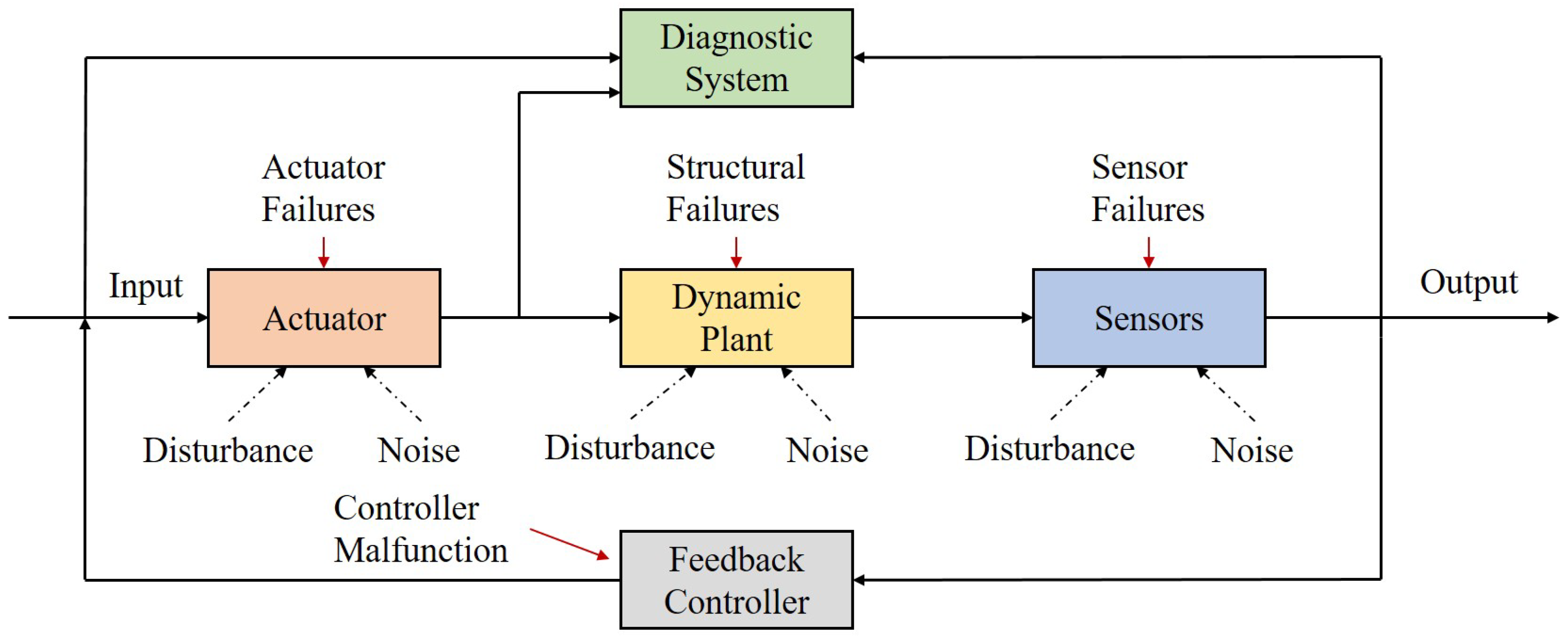
1.1. Background

Compared to passive fault-tolerant control, taking fault into account as a system perturbation, FDD is an active strategy for detecting and identifying potential abnormalities and faults, providing early warning, and recommending corrective actions to prevent failure occurrence. Compared to prognostics, dealing with fault prediction before it occurs, diagnostics is a posterior event analysis and it is required after occurring a fault. In harsh working environments, such as extreme temperatures, high pressure, and underwater, sensors are prone to faults, while the sensor is an essential component of data acquisition systems, sensor faults, including incipient failure and abrupt failure, will affect the accuracy, stability, and reliability. It has become essential for industrial applications, especially for engineering systems such as mechanical engineering [1,2,3,4], electric vehicle dynamics [5,6], power electronic systems [7,8,9,10], electric machines [11,12,13,14], and wind energy conversion systems [15,16,17,18]. The task of FDD is to spot process abnormalities promptly and identify their early causes [19]. The elements of a general structure for fault diagnosis system and control system are shown in Figure 1. It demonstrates different components in a control loop, and failures could exist in actuators, dynamic plants, sensors, and feedback controllers.

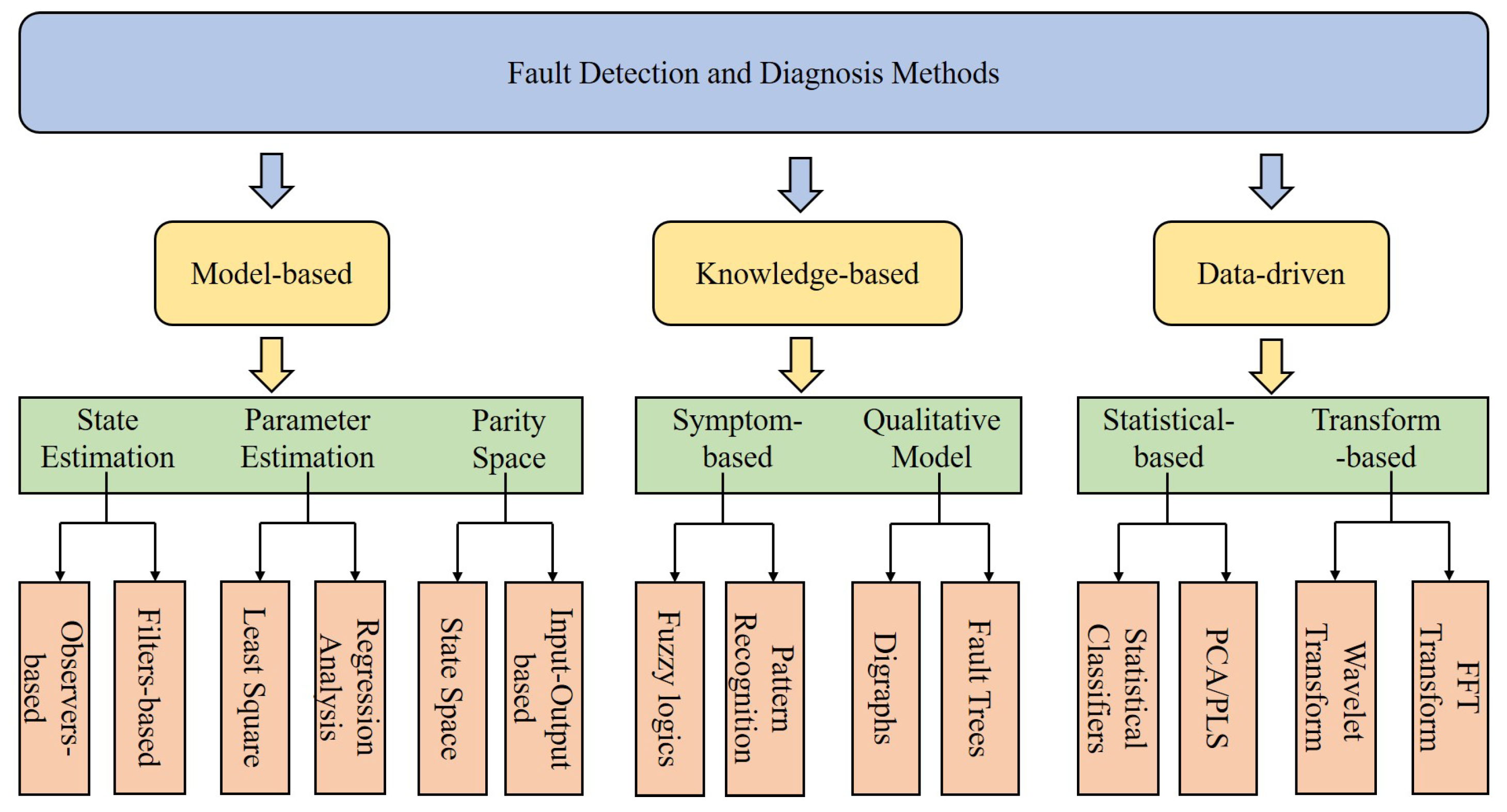
1.2. Evolution of Fault Detection and Diagnosis

Generally, approaches to detecting and diagnosing faults can be divided into three categories, as shown in Figure 2.

1.2.1. Model-Based Methods

Model-based methods include state estimation, parameter estimation, and parity space. The model-based methods utilize physical and mathematical knowledge and they possess the explainability for making decisions in a transparent way rather than in a black box [20,21,22]. However, the noisy operation environment hinders physics-based modeling and degrades the accuracy of complex dynamic modeling [23,24].

1.2.2. Knowledge-Based Methods

Knowledge-based methods include symptom-based methods and qualitative methods. The knowledge-based methods are usually implemented by experts, and the fault diagnosis relies on the accumulation of prior information and logical reference [25]. These methods are efficient within the scope of existing knowledge and struggle to tackle unexpected failures.

1.2.3. Data-Driven Methods

Data-driven methods include statistical-based methods and transform-based methods. Compared to model-based methods and knowledge-based methods, data-driven approaches are efficient when confronted with high-dimensional data. They require a sufficient quantity of data and enhance accuracy by extracting information or features from large-scale datasets [26,27]. Yet the lack of an accurate mathematical model makes it inadequate for detecting incipient faults.

The Internet of Things era revolutionizes industrial processes by collecting a large amount of information via a network of terminals, leading to a data explosion and the rocketing complexity of model construction. Troubleshooting highly complex systems involves multiple processes and multiple anomalies, making conventional physics-based deterministic modeling more challenging. Moreover, implementing the knowledge-based FDD methods relies heavily on expertise or prior information, which is time-consuming and labor-intensive especially when dealing with a high-dimensional process. Data-driven approaches are targeted for addressing large-scale data and extracting features from data.

The statistical approach is a branch of data-driven schemes, and extracts the process information from measurement or observation. Its significant advantage is that it can tackle many highly correlated variables without complex mathematical forms or costly design efforts. Statistical methods [28] have gained popularity in practical applications for their ability to directly analyze input and output data, particularly PCA [29,30,31,32,33] and PLS [34,35,36,37]. PCA, PLS, and independent component analysis (ICA) are traditional statistical analysis methods based on deterministic models. The underlying theoretical foundation of traditional multivariate analysis is linear algebra.

In practice, industrial process data are polluted by missing data and outliers, which can significantly influence the accuracy of features and control thresholds. The probabilistic extensions of traditional statistical methods employ distributions to describe states to enhance their ability to process sampling data with disturbances, outliers, and missing values. In addition, the probabilistic form of statistical analysis can employ non-linear data and thus can be applied in industrial processes. Recently, the probabilistic counterparts of PCA [38] and factor analysis (FA) [39] have been generated for fault diagnosis. Furthermore, the extensions of their mixture form with multiple operation modes have been generalized [40].

The study on statistical-based fault diagnosis methods draws remarkable research attention. Due to their similarity in collecting, processing, and extracting information from data, these strategies are viewed as statistical-based methods. In this context, these schemes are mainly characterized as follows:

(1)

Without a complex model construction, a statistical-based FDD design can extract the information and make decisions directly on the sampling data.

(2)

These strategies are designed to address FDD in static or dynamic systems in a stable state with the flexible application of statistical tests and their mixed indices.

1.3. Motivation and Contribution

Statistical-based fault diagnosis has attracted attention in industrial applications and the academic community. The sensor technology gives rise to a data explosion, and the data quality significantly impacts the modeling of the process and thus influences the performance of fault diagnosis. Probabilistic extensions of conventional statistical methods spring up due to their robustness and advantages in treating outliers, disturbance, and missing values. There is no comprehensive review of statistical FDD methods under a probabilistic framework. Therefore, statistical methods with a probabilistic model are an unavoidable element that needs to be addressed in industrial applications and the academic community. Different from other reviews on FDD [41,42,43], this review focuses on detailed explanations to let readers understand the principle of each method and save some time searching a lot of references. The purpose of this review is to provide theoretical background and recent application instances of probabilistic-based statistical fault diagnosis.

1.4. Organization of This Paper

The remainder of this paper is organized as follows. The theoretical background of the probabilistic model is presented in Section 2. Section 3 gives a brief overview of the probabilistic extensions of statistical methods and their practical applications. The challenges and perspectives are demonstrated in Section 4. Conclusions are finally drawn in Section 5.

2. Theoretic Background

Maximum likelihood estimation (MLE) and Bayesian theory are employed when the probabilistic model is introduced into statistical methods. This section will briefly introduce the principles of MLE and Bayesian inference.

2.1. Maximum Likelihood Estimation

In statistics, MLE estimates the parameters of an assumed probability distribution with observation measurement and maximizes the probability [44]. MLE is generated to find the probability density function (PDF) that is most likely to produce a data sample given the observation. The data $\mathbf{y}=(y_1,y_2,\cdots ,y_m)$ is a random sample from an unknown population. In practice, the model usually involves abundant parameters, and the likelihood function is probably nonlinear, making it difficult to obtain an analytic solution. A nonlinear model is established to estimate the remaining useful life of a system, where the unknown parameters are estimated with the help of MLE [45].

The $\mathbf{v}=(v_1,v_2,\cdots ,v_k)$ is a vector defined on a multi-dimensional parameter space. $p\left(\mathbf{y}\right|\mathbf{v})$ denotes the probability of y given v. The likelihood function is defined by [46]

$$\begin{array}{c}\hfill L\left(\mathbf{v}\right|\mathbf{y})=p(\mathbf{y}\left|\mathbf{v}\right).\end{array}$$

(1)

The MLE estimate is obtained by maximizing the log-likelihood function. Assuming that the log-likelihood $lnL\left(\mathbf{v}\right|\mathbf{y})$ is differentiable, if ${\mathbf{v}}_{MLE}$ exists, it must satisfy Equation (2):

$$\begin{array}{c}\hfill \frac{\partial logL\left(\mathbf{v}\right|\mathbf{y})}{\partial v_i}=0.\end{array}$$

(2)

$L\left(\mathbf{v}\right|\mathbf{y})$ and $p\left(\mathbf{y}\right|\mathbf{v})$ are defined on different axes, that $p\left(\mathbf{y}\right|\mathbf{v})$ is a function of the data given parameters, defined on the data scale, and $L\left(\mathbf{v}\right|\mathbf{y})$ is defined on the parameter scale.

2.2. Bayesian Learning

Bayesian learning provides a rigorous framework for complex nonlinear systems whose internal state variables are inaccessible to direct measurement. Given a general discrete-time state estimation equation and measurement function,

$$\begin{array}{c}\hfill {\mathbf{x}}_k=g\left({\mathbf{x}}_{k-1}\right)+{\mathbf{e}}_k,\end{array}$$

(3)

$$\begin{array}{c}\hfill {\mathbf{y}}_k=h\left({\mathbf{x}}_k\right)+{\mathbf{v}}_k,\end{array}$$

(4)

where ${\mathbf{x}}_k\in {\mathbb{R}}^n$ is the state at time step k, ${\mathbf{e}}_k\in {\mathbb{R}}^n$ is the process noise, and $g:{\mathbb{R}}^n\to {\mathbb{R}}^n$ denotes the transition function. ${\mathbf{y}}_k\in {\mathbb{R}}^p$ is the measurement, ${\mathbf{v}}_k\in {\mathbb{R}}^p$ is the measurement noise, and $h:{\mathbb{R}}^n\to {\mathbb{R}}^p$. ${\mathbf{e}}_k$ and ${\mathbf{v}}_k$ are independent.

The Bayesian learning is to recursively estimate the PDF of ${\mathbf{x}}_k$ given measurements ${\mathbf{y}}_k$. The initial density is determined beforehand, and $p\left({\mathbf{x}}_k\right|{\mathbf{x}}_{k-1})$ denotes the transition probability density. The inference of the state ${\mathbf{x}}_k$ relies on the marginal density $p\left({\mathbf{x}}_k\right|{\mathbf{y}}_{1:k})$. The predictive function of ${\mathbf{x}}_k$ at step k is estimated by [47]

$$\begin{array}{c}\hfill p\left({\mathbf{x}}_k\right|{\mathbf{y}}_{1:k-1})=\int p\left({\mathbf{x}}_k\right|{\mathbf{x}}_{k-1})p\left({\mathbf{x}}_{k-1}\right|{\mathbf{y}}_{1:k-1})\mathrm{d}{\mathbf{x}}_{k-1}.\end{array}$$

(5)

Then, the marginal filtering density is computed

$$\begin{array}{c}\hfill p\left({\mathbf{x}}_k\right|{\mathbf{y}}_{1:k})=\frac{p\left({\mathbf{y}}_k\right|{\mathbf{x}}_k)p\left({\mathbf{x}}_k\right|{\mathbf{y}}_{1:k-1})}{p\left({\mathbf{y}}_k\right|{\mathbf{y}}_{1:k-1})},\end{array}$$

(6)

where $p\left({\mathbf{y}}_k\right|{\mathbf{y}}_{1:k-1})$ is the normalizing parameter.

A Bayesian network is a probabilistic graphical model that illustrates the relationships between variables.

$$\begin{array}{c}\hfill p(\mathbf{a},\mathbf{b})=p\left(\mathbf{a}\right|\mathbf{b})·p(\mathbf{b}),\end{array}$$

(7)

and the joint probability distribution for a Bayesian network with nodes $\mathbf{a}=\{a_1,\cdots ,a_n\}$ is given by

$$\begin{array}{c}\hfill p\left(\mathbf{a}\right)=\prod _{i=1}^{n}p\left(a_i\right|parents\left(a_i\right)),\end{array}$$

(8)

where $parents\left(a_i\right)$ is the parent set of node $a_i$.

Research based on Bayesian learning has attracted huge attention in the field of fault diagnosis. Zhao proposed advanced Bayesian estimation algorithms to monitor the faulty sensors [48], then improved algorithms for online ability and correlated signals in nonlinear processes, respectively, [49,50]. Bayesian network is adopted in fault diagnosis [51,52,53,54,55,56,57,58,59,60,61]. Multivariate statistical analysis has been combined with Bayesian inference for fault detection and isolation [62]. A Bayesian maximum likelihood classifier is validated as accurate for induction machine and stator short circuit fault diagnosis [63]. The probabilistic Bayesian deep learning framework exploits the risk-aware model to identify unknown faults and enhance the trustworthiness of the diagnostic results [64,65].

3. Probabilistic Statistical-Based Approaches

This section discusses different kinds of static statistical-based approaches. Four probabilistic models applied in the field of FDD are illustrated, including probabilistic PCA, probabilistic PLS, probabilistic ICA, probabilistic canonical correlation analysis (CCA), and probabilistic Fisher discriminant analysis (FDA). PCA extracts the principal components that are retained to explain the majority of the variability in the data by maximizing the variance. Compared to PCA, the FDA maximizes the separation among classes while minimizing the separation between classes. The components after PCA decomposition are orthogonal and therefore irrelevant, but independence is not guaranteed. Compared to PCA, ICA can find the original components in the observed mixtures, and it is a linear transformation of the data in the original feature space. PCA involves only one set of variables, while CCA extends to the interdependence between two sets of variables, measuring the correlation between the two sets of variables. The probabilistic approaches of traditional statistical analysis are shown in Figure 3. They differ in the variable distribution, the application scenario, and whether the dataset is labeled. PPCA and PICA have the same characteristics, they can deal with non-Gaussian distribution data and stationary processes. PFDA and PPLS are supervised methods. PCCA excels in other methods of tackling dynamic processes. The probabilistic extensions of traditional multivariate statistical analysis still retain original characteristics and broaden the range of applications.

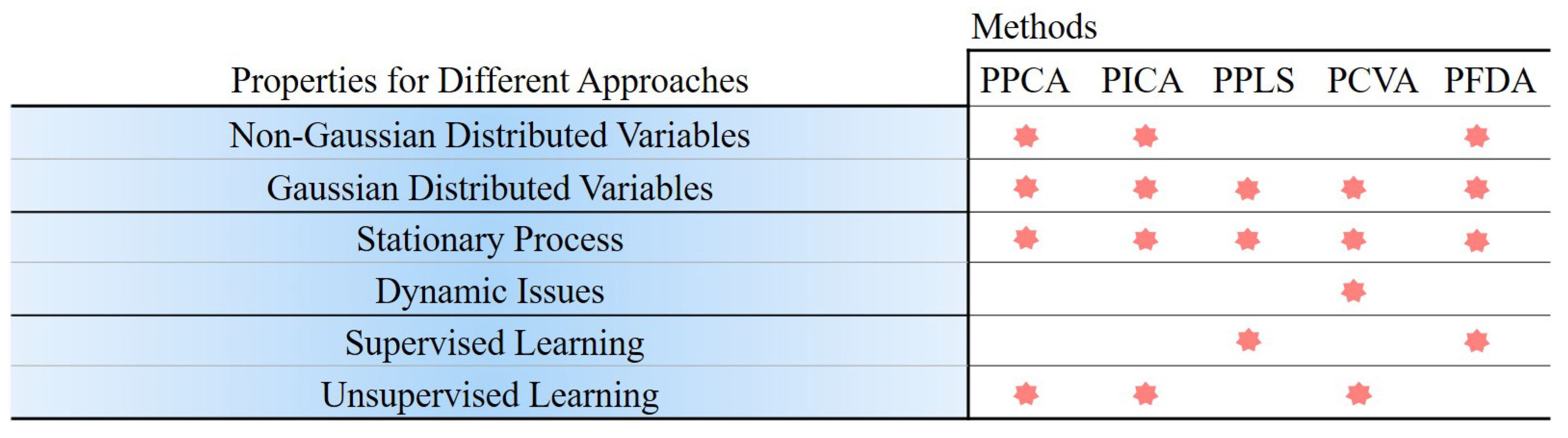
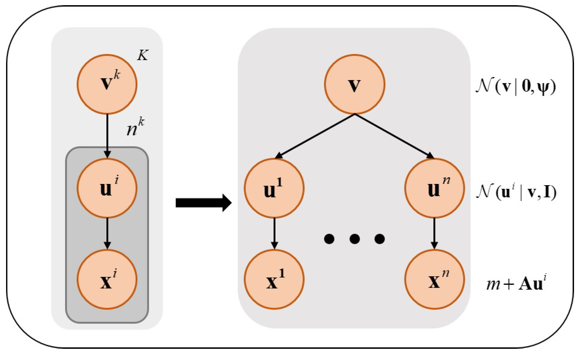
3.1. Probabilistic Principal Component Analysis

PCA is a technique targeted for dimensionality reduction, and it has wide applications, including data compression, image processing, data analysis, and pattern recognition [66,67,68,69]. The probabilistic derivation of PCA is given by

$$\begin{array}{c}\hfill \mathbf{y}=\mathbf{W}\mathbf{t}+\mathbf{m}+\mathit{ϵ},\end{array}$$

(9)

where $\mathbf{y}\in {\mathbb{R}}^d$, independent unobservable variable $\mathbf{t}\in {\mathbb{R}}^q\sim \mathcal{N}(0,\mathbf{I})$, and $q<d$. The transition matrix is $\mathbf{W}\in {\mathbb{R}}^{d\times q}$, and the vector is $\mathbf{m}\ne 0$. The key assumption for PPCA is that the noise in this probability model is likewise Gaussian $\mathit{ϵ}\sim \mathcal{N}(\mathbf{0},\mathrm{\Psi })$ and the covariance $\mathrm{\Psi }={\sigma }^2\mathbf{I}$ is constrained to be a diagonal matrix, so that $\mathbf{y}$ are conditionally independent given the values of $\mathbf{t}$. The conditional PDF of $\mathbf{y}$ and the marginal PDF of $\mathbf{t}$ obtained by integration are implied by

$$\begin{array}{cc}\hfill & \mathbf{y}|\mathbf{t}\sim \mathcal{N}(\mathbf{W}\mathbf{t}+\mathbf{m},{\sigma }^2\mathbf{I}),\hfill \end{array}$$

(10)

$$\begin{array}{cc}\hfill & \mathbf{y}\sim \mathcal{N}(\mathbf{m},\mathbf{A}),\hfill \end{array}$$

(11)

where $\mathbf{A}=\mathbf{W}{\mathbf{W}}^T+{\sigma }^2\mathbf{I}$, then the log-likelihood function is

$$\begin{array}{cc}\hfill & \mathcal{L}=-\frac{N}{2}\{ln|\mathbf{A}|+tr\left({\mathbf{A}}^{-1}\mathbf{S}\right)+dln\left(2\pi \right)\},\hfill \end{array}$$

(12)

$$\begin{array}{cc}\hfill & \mathbf{S}=\frac{1}{N}\sum _{n=1}^N({\mathbf{y}}_n-\mathbf{m}){({\mathbf{y}}_n-\mathbf{m})}^T.\hfill \end{array}$$

(13)

Estimates for $\mathbf{W}$ and ${\sigma }^2$ is obtained by iteratively maximizing Equation (12) by employing the EM algorithm [70].

$$\begin{array}{cc}\hfill {\mathbf{W}}_{ML}& ={\mathbf{U}}_q{({\mathbf{\Lambda }}_q-{\sigma }^2\mathbf{I})}^{\frac{1}{2}}\mathbf{R},\hfill \end{array}$$

(14)

$$\begin{array}{cc}\hfill {\sigma }_{ML}^2& =\frac{1}{d-q}\sum _{j=q+1}^d{\lambda }_j,\hfill \end{array}$$

(15)

where the first qth column vectors in ${\mathbf{U}}_q\in {\mathbb{R}}^{d\times q}$ are the qth principal eigenvectors of $\mathbf{S}$, with corresponding eigenvalues ${\lambda }_i,\cdots ,{\lambda }_q$ in the diagonal matrix ${\mathbf{\Lambda }}_q\in {\mathbb{R}}^{q\times q}$, and $\mathbf{R}\in {\mathbb{R}}^{q\times q}$ is an arbitrary orthogonal matrix. Note that ${\mathbf{U}}_q$ and ${\mathbf{\Lambda }}_q$ can be obtained by performing the singular value decomposition on $\mathbf{S}$.

The conditional distribution of the latent variable $\mathbf{t}$ given the observed $\mathbf{y}$ is obtained with the help of Bayesian inference

$$\begin{array}{cc}\hfill \mathbf{t}|\mathbf{y}\sim \mathcal{N}& ({\mathbf{B}}^{-1}{\mathbf{W}}^T(\mathbf{y}-\mathbf{m}),{\sigma }^2{\mathbf{B}}^{-1}),\hfill \end{array}$$

(16)

where $\mathbf{B}={\mathbf{W}}^T\mathbf{W}+{\sigma }^2\mathbf{I}$. From Equation (16), the point-wise technique can be employed when the conditional distribution is generated

$$\begin{array}{c}\hfill \langle \mathbf{t}|\mathbf{y}\rangle ={\mathbf{B}}^{-1}{\mathbf{W}}_{ML}^T(\mathbf{y}-\mathbf{m}).\end{array}$$

(17)

Then, the high-dimensional observed data $\mathbf{y}$ can be condensed into a new distribution $\mathbf{t}$ which satisfies Gaussian.

The probabilistic PCA model has abundant modifications and extensions to be applied for fault diagnosis. Choi et al. proposed a fault detection scheme based on a maximum-likelihood PCA mixture model [40]. To address the challenge of separating several factors that together cause a failure to occur, probabilistic PCA was created [71]. An aligned mixture probabilistic PCA is proposed by Yang for fault detection of multimode chemical processes [72]. Then, a reconstruction-based multivariate contribution analysis is applied to the PPCA mixture model for fault isolation [73].

The robust version of probabilistic PCA is modified to deal with outliers and missing data during the modeling stage [74]. In addition, a variational inference process based on the Bayesian PCA model structure provides the foundation of a defect reconstruction method [75]. Additionally, the hidden Markov model framework temporally extends the static mixture probabilistic PCA model-based classifier to the dynamic form [76,77]. It was suggested to use a hybrid framework that takes into account moving window PCA and Bayesian networks to cope with barely accessible data in a fault state [78].

By thoroughly analyzing the principle and implementation of probabilistic PCA, the significant advantages can be summarized as follows.

(1)

Enhanced Robustness: In practical applications, disturbances are unavoidable in a complex working environment. Probabilistic PCA disposes of the problem that sampling data are mixed with outliers and missing values by using distribution modeling of these data and enhancing robustness.

(2)

Increased Complex Data: The introduced latent variables enable probabilistic PCA to process non-linear data, improving the performance of dimensional reduction.

(3)

Probability Inference: Probabilistic PCA is a dimensionality reduction method based on probability models. It provides quantitative information on uncertainty and probabilistic inferences to obtain more accuracy and effectiveness. Ultimately, the ability to interpret data is substantially intensified.

3.2. Probabilistic Partial Least Squares

The core of the probabilistic PLS model is to use a part of the latent variables to explain the observed data set. The probabilistic PLS model is formulated by [79]

$$\begin{array}{cc}\hfill \mathbf{x}& ={\mathbf{m}}_x+\mathbf{J}{\mathbf{t}}^s+\mathbf{Q}{\mathbf{t}}^b+{\mathit{ϵ}}_x,\hfill \end{array}$$

(18)

$$\begin{array}{cc}\hfill \mathbf{y}& ={\mathbf{m}}_y+\mathbf{K}{\mathbf{t}}^s+{\mathit{ϵ}}_y,\hfill \end{array}$$

(19)

where $\mathbf{J}\in {\mathbb{R}}^{m\times q_s}$, $\mathbf{K}\in {\mathbb{R}}^{r\times q_s}$ and $\mathbf{Q}\in {\mathbb{R}}^{m\times q_b}$; ${\mathbf{t}}^s\in {\mathbb{R}}^{q_s\times 1}$, ${\mathbf{t}}^b\in {\mathbb{R}}^{q_b\times 1}$; ${\mathbf{m}}_x$ and ${\mathbf{m}}_y$ are the mean of $\mathbf{x}$ and $\mathbf{y}$; and ${\mathit{ϵ}}_x$ and ${\mathit{ϵ}}_y$ denotes measurement noises of $\mathbf{x}$ and $\mathbf{y}$, respectively.

In the probabilistic PLS model, ${\mathbf{t}}^s\sim \mathcal{N}(\mathbf{0},\mathbf{I})$, ${\mathbf{t}}^b\sim \mathcal{N}(\mathbf{0},\mathbf{I})$, ${\mathit{ϵ}}_x\sim \mathcal{N}(\mathbf{0},{\mathbf{\Sigma }}_x)$, and ${\mathit{ϵ}}_y\sim \mathcal{N}(\mathbf{0},{\mathbf{\Sigma }}_y)$. Different from the probabilistic PCA model that assumes the error covariance matrix to be a diagonal matrix with a constant value, different noise variances have been assumed for different variables ${\mathbf{\Sigma }}_x=diag{\left\{{\sigma }_{x,u}^2\right\}}_{u=1,2,\cdots ,m}$ and ${\mathbf{\Sigma }}_y=diag{\left\{{\sigma }_{y,v}^2\right\}}_{v=1,2,\cdots ,r}$. Given data sets $\mathbf{X}={[{\mathbf{x}}_1,{\mathbf{x}}_2,\cdots ,{\mathbf{x}}_n]}^T\in {\mathbb{R}}^{n\times m}$ and $\mathbf{Y}={[{\mathbf{y}}_1,{\mathbf{y}}_2,\cdots ,{\mathbf{y}}_n]}^T\in {\mathbb{R}}^{n\times r}$, the log-likelihood function can be determined by

$$\begin{array}{cc}\hfill & L(\mathbf{X},\mathbf{Y}|{\mathbf{m}}_x,{\mathbf{m}}_y,\mathbf{J},\mathbf{Q},\mathbf{K},{\mathbf{\Sigma }}_x,{\mathbf{\Sigma }}_y)\hfill \\ \hfill =ln& {\displaystyle \prod _{i=1}^n}p({\mathbf{x}}_i,{\mathbf{y}}_i|{\mathbf{m}}_x,{\mathbf{m}}_y,\mathbf{J},\mathbf{Q},\mathbf{K},{\mathbf{\Sigma }}_x,{\mathbf{\Sigma }}_y).\hfill \end{array}$$

(20)

The optimal values of parameters are determined by the EM algorithm:

$$\begin{array}{cc}\hfill & {\mathbf{J}}^{new}=\left[\sum _{i=1}^n{\mathbf{x}}_{i}E{\left({\mathbf{t}}_i^s\mid \left[\begin{array}{c}{\mathbf{x}}_i\\ {\mathbf{y}}_i\end{array}\right]\right)}^T\right]{\left[\sum _{i=1}^{n}E\left({\mathbf{t}}_i^s{{\mathbf{t}}_i^s}^T\mid \left[\begin{array}{c}{\mathbf{x}}_i\\ {\mathbf{y}}_i\end{array}\right]\right)\right]}^{-1},\hfill \end{array}$$

(21)

$$\begin{array}{cc}\hfill & {\mathbf{Q}}^{new}=\left[\sum _{i=1}^n{\mathbf{x}}_{i}E{\left({\mathbf{t}}_i^b\mid \left[\begin{array}{c}{\mathbf{x}}_i\\ {\mathbf{y}}_i\end{array}\right]\right)}^T\right]{\left[\sum _{i=1}^{n}E\left({\mathbf{t}}_i^b{{\mathbf{t}}_i^b}^T\mid \left[\begin{array}{c}{\mathbf{x}}_i\\ {\mathbf{y}}_i\end{array}\right]\right)\right]}^{-1},\hfill \end{array}$$

(22)

$$\begin{array}{cc}\hfill & {\mathbf{K}}^{new}=\left[\sum _{i=1}^n{\mathbf{y}}_{i}E{\left({\mathbf{t}}_i^s\mid \left[\begin{array}{c}{\mathbf{x}}_i\\ {\mathbf{y}}_i\end{array}\right]\right)}^T\right]{\left[\sum _{i=1}^{n}E\left({\mathbf{t}}_i^s{{\mathbf{t}}_i^s}^T\mid \left[\begin{array}{c}{\mathbf{x}}_i\\ {\mathbf{y}}_i\end{array}\right]\right)\right]}^{-1},\hfill \end{array}$$

(23)

$$\begin{array}{cc}\hfill & {\mathbf{\Sigma }}_x^{new}=\frac{1}{n}diag\left\{\sum _{i=1}^n\left[{\mathbf{x}}_i{\mathbf{x}}_i^T-\left[{\mathbf{J}}^{new}{\mathbf{Q}}^{new}\right]E\left({\mathbf{t}}_i^s|\left[\begin{array}{c}{\mathbf{x}}_i\\ {\mathbf{y}}_i\end{array}\right]\right){\mathbf{y}}_i^T\right]\right\},\hfill \end{array}$$

(24)

$$\begin{array}{cc}\hfill & {\mathbf{\Sigma }}_y^{new}=\frac{1}{n}diag\left\{\sum _{i=1}^n\left[{\mathbf{y}}_i{\mathbf{y}}_i^T-{\mathbf{K}}^{new}E\left({\mathbf{t}}_i^s|\left[\begin{array}{c}{\mathbf{x}}_i\\ {\mathbf{y}}_i\end{array}\right]\right){\mathbf{y}}_i^T\right]\right\}.\hfill \end{array}$$

(25)

The supervised model PPLS builds a regression model between two sets of variables. For further applications, the probabilistic PLS model has been modified. On the basis of this, the validity of the classification of an unknown item is assessed [80]. Zheng adapted the probabilistic PLS model to the semi-supervised version for the creation of soft sensors [81]. Data-driven fault identification and diagnosis techniques are proposed based on a novel locally weighted probabilistic kernel PLS [82]. Botella described an improvement to discriminant partial least squares that use the kernel trick and Bayes rule to implement data classification [83]. To further decompose the PPLS model, a concurrent probabilistic PLS approach is suggested, and monitoring statistics are created for assessment [84].

Compared with traditional PLS, probabilistic PLS treats independent and dependent variables as random variables and assumes that they satisfy the Gaussian distribution. The probabilistic model is capable of dealing with disturbance, outliers, and missing data and then improving the stability and prediction accuracy of the model.

3.3. Probabilistic Independent Component Analysis

ICA separates the dataset into linear combinations of statistically independent non-Gaussian sources. It is a significant application of the blind source separation method. The probabilistic ICA model is [85]

$$\begin{array}{c}\hfill {\mathbf{x}}_n=\mathbf{A}{\mathbf{s}}_n+{\mathit{ϵ}}_n,\end{array}$$

(26)

where ${\mathbf{x}}_n$ is the observation, ${\mathbf{s}}_n$ is a statistically independent non-Gaussian source, $\mathit{ϵ}\sim \mathcal{N}(\mathbf{0},{\beta }^{-1}\mathbf{I})$ denotes the noise vector, and $\mathbf{A}$ represent a linear transformation. The likelihood can be given by

$$\begin{array}{c}\hfill p\left({\mathbf{x}}_n\right|{\mathbf{s}}_n,\mathbf{A},\beta )=\sqrt{\frac{\beta }{2\pi }}{e}^{\left(\frac{\beta }{2}\right){({\mathbf{x}}_n-\mathbf{A}{\mathbf{s}}_n)}^T({\mathbf{x}}_n-\mathbf{A}{\mathbf{s}}_n)}.\end{array}$$

(27)

Due to the adaptive tails in the Student’s t probability model, the Student’s t distribution can approach the distribution of non-Gaussian sources. The sources used by the Student’s t might be described as

$$\begin{array}{cc}\hfill p\left(s_n^j\right)& =t(s_n^j|0,{\sigma }_j^2,{\nu }_j)\hfill \\ & =\frac{\Gamma \left(\frac{{\nu }_j+1}{2}\right)}{\Gamma \left(\frac{{\nu }_j}{2}\right)\sqrt{{\nu }_j\pi {\sigma }_j^2}}{\left(1+\frac{{\left(s_n^j\right)}^2}{{\nu }_j{\sigma }_j^2}\right)}^{-\frac{({\nu }_j+1)}{2}}\hfill \\ \hfill & ={\int }_0^{\infty }\mathcal{N}(s_n^j|0,{\left(u_n^j\right)}^{-1}{\sigma }_j^2)Ga(u_n^j|a_n^j,b_n^j)d{u}_n^j,\hfill \end{array}$$

(28)

where $Ga(·)$ represent the Gamma distribution. To estimate the non-Gaussian variables, one can use the variational Bayesian EM approach. Defining $\mathbf{F}\sim \{\mathbf{S},\mathbf{U}\}$ for latent variables, the log-likelihood is given by

$$\begin{array}{c}\hfill logp\left(\mathbf{X}\right|\mathit{\theta })=log\frac{p(\mathbf{F},\mathbf{X}|\mathit{\theta })}{p\left(\mathbf{F}\right|\mathbf{X},\mathit{\theta })}.\end{array}$$

(29)

By introducing an auxiliary distribution $q\left(\mathbf{F}\right)$ as the approximation distribution, we have

$$\begin{array}{cc}\hfill & log\frac{p(\mathbf{F},\mathbf{X}|\mathit{\theta })}{p\left(\mathbf{F}\right|\mathbf{X},\mathit{\theta })}\hfill \end{array}$$

(30)

$$\begin{array}{ll}& \hspace{1em}\hspace{1em}\hspace{1em}\hspace{1em}\hspace{1em}=log\int q\left(\mathbf{F}\right)\frac{p(\mathbf{F},\mathbf{X}|\mathit{\theta }\left)q\right(\mathbf{F})}{p\left(\mathbf{F}\right|\mathbf{X},\mathit{\theta }\left)q\right(\mathbf{F})}\mathrm{d}\mathbf{F}\end{array}$$

(31)

$$\begin{array}{ll}& \hspace{1em}\hspace{1em}\hspace{1em}\hspace{1em}\hspace{1em}\hspace{1em}\hspace{1em}\hspace{1em}\hspace{1em}\hspace{1em}\ge \int q\left(\mathbf{F}\right)\left\{log\frac{p(\mathbf{F},\mathbf{X}|\mathit{\theta })}{q\left(\mathbf{F}\right)}-log\frac{p\left(\mathbf{F}\right|\mathbf{X},\mathit{\theta })}{q\left(\mathbf{F}\right)}\right\}\mathrm{d}\mathbf{F}\end{array}$$

(32)

$$\begin{array}{ll}& \hspace{1em}\hspace{1em}\hspace{1em}\hspace{1em}=F\left(q\right(\mathbf{F}),\mathit{\theta })+KL\left(q\right|\left|p\right)\end{array}$$

(33)

$$\begin{array}{ll}& \ge F\left(q\right(\mathbf{F}),\mathit{\theta }).\end{array}$$

(34)

For variational Bayesian, the latent distributions are assumed as independent $q\left(\mathbf{F}\right)\approx q\left(\mathbf{S}\right)q\left(\mathbf{U}\right)$. Then, taking the derivative of the lower bound with respect to $q\left(\mathbf{S}\right)$, $q\left(\mathbf{U}\right)$, $q\left(\mathbf{A}\right)$, $q\left(\beta \right)$, and $q\left({\nu }_j\right)$.

$$\begin{array}{c}\hfill \frac{\partial F\left(q\right(\mathbf{F}),\mathit{\theta })}{\partial q\left(\mathbf{S}\right)}=-\frac{\beta }{2}({\mathbf{x}}_n^T{\mathbf{x}}_n-2{\mathbf{A}}^T{\mathbf{x}}_n{\mathbf{s}}_n+{\mathbf{A}}^T\mathbf{A}{\mathbf{s}}_n^2)-\frac{1}{2}diag\left(〈{\mathbf{u}}_n〉\right){\mathbf{s}}_n^2,\end{array}$$

(35)

where $〈{\mathbf{u}}_n〉={\left[〈u_n^1〉,〈u_n^2〉,\cdots ,〈u_n^d〉\right]}^T$, on the basis of conjugate exponential distribution, $q\left(\mathbf{S}\right)\sim {\displaystyle \prod _{n=1}^N}\left({\mathbf{s}}_n|{\overline{\mathbf{s}}}_n,{\overline{\mathbf{\Sigma }}}_s^n\right)$, the parameters can be obtained as

$$\begin{array}{cc}\hfill {\overline{\mathbf{\Sigma }}}_s^n=& {\left[diag\left(〈{\mathbf{u}}_n〉\right)+\beta {\mathbf{A}}^T\mathbf{A}\right]}^{-1},\hfill \end{array}$$

(36)

$$\begin{array}{ll}{\overline{\mathbf{s}}}_n=& \beta {\overline{\mathbf{\Sigma }}}_s^n{\mathbf{A}}^T{\mathbf{x}}_n.\hfill \end{array}$$

(37)

Similarly, by defining $q\left(\mathbf{U}\right)={\displaystyle \prod _{j=1}^d}{\displaystyle \prod _{n=1}^N}Ga\left(u_n^j\right|{\overline{a}}_{u_n^j},{\overline{b}}_{u_n^j})$, we obtain

$$\begin{array}{c}\hfill \frac{\partial F\left(q\right(\mathbf{F}),\mathit{\theta })}{\partial q\left(\mathbf{U}\right)}=\left(\frac{{\nu }_j-1}{2}\right)log{u}_n^j-\frac{1}{2}\left({〈s_n^j〉}^2+{\nu }_j{\sigma }_j^2\right)u_n^j.\end{array}$$

(38)

We have

$$\begin{array}{cc}\hfill & {\overline{a}}_{u_n^j}={\nu }_j+1,\hfill \end{array}$$

(39)

$$\begin{array}{cc}\hfill & {\overline{b}}_{u_n^j}=\frac{{\langle s_n^j\rangle }^2+{\nu }_j{\sigma }_j^2}{{\nu }_j+1}.\hfill \end{array}$$

(40)

Other parameters can be derived by taking the differentiation concerning $\mathbf{A}$, $\beta$, and ${\nu }_j$

$$\begin{array}{cc}\hfill \mathbf{A}& =\left[\sum _{n=1}^N\langle s_n\rangle {\mathbf{x}}_n^T\right]{\left[\sum _{n=1}^N\langle s_n{s}_n^T\rangle \right]}^{-1},\hfill \end{array}$$

(41)

$$\begin{array}{cc}\hfill \beta & =ND{\left(\sum _{n=1}^N\sum _{n=1}^D〈{(x_n^i-{\mathbf{a}}_i^T{\mathbf{s}}_n)}^2〉\right)}^{-1},\hfill \end{array}$$

(42)

where $x_n^i$ is the ith element of observation and ${\mathbf{a}}_i$ is the ith column of $\mathbf{A}$, while the degree of freedom ${\nu }_j$ can be induced by solving the following nonlinear formula:

$$\begin{array}{c}\hfill 1+\frac{N}{2}log\frac{{\nu }_j}{2}-\psi \left(\frac{{\nu }_j}{2}\right)+log{\sigma }_j^2+\frac{1}{2}\sum _{n=1}^N(〈log{u}_n^j-{\sigma }_j^2\langle u_n^j\rangle 〉)=0.\end{array}$$

(43)

The expectations involved in Equation (43) are given by

$$\begin{array}{cc}\hfill & \langle u_n^j\rangle ={\left({\overline{b}}_{u_n^j}\right)}^{-1},\hfill \end{array}$$

(44)

$$\begin{array}{cc}\hfill {\langle s_n^j\rangle }^2& ={\langle {\mathbf{s}}_n{{\mathbf{s}}_n}^T\rangle }_{jj}={\left({\overline{\mathbf{s}}}_n{{\overline{\mathbf{s}}}_n}^T+{\overline{\mathbf{\Sigma }}}_s^n\right)}_{jj},\hfill \end{array}$$

(45)

$$\begin{array}{cc}\hfill \langle log{u}_n^j\rangle & =\psi \left({\nu }_j\right)-log\frac{{\nu }_j}{2}-log{\overline{b}}_{u_n^j}.\hfill \end{array}$$

(46)

Traditional ICA methods are limited in their ability to process non-Gaussian distributed signals, resulting in inaccurate decomposition results. Probabilistic ICA uses probability distributions to solve the above-mentioned problem. Probabilistic ICA can better process non-Gaussian signals because of its ability to model different probability distributions. In addition, probabilistic ICA employs the variational Bayesian method to estimate the uncertainty of the separation variable and improve the robustness and interpretability of the model.

3.4. Probabilistic Canonical Correlation Analysis

Given two random vectors, canonical correlation analysis (CCA) is concerned with finding projections such that the components within one set of projections are correlated with components in the other set. The probabilistic extension of CCA is given by [86].

$$\begin{array}{cc}\hfill {\mathbf{x}}_1=& {\mathbf{W}}_1\mathbf{z}+{\mathbf{m}}_1+{\mathit{ϵ}}_1,\hfill \end{array}$$

(47)

$$\begin{array}{cc}\hfill {\mathbf{x}}_2=& {\mathbf{W}}_2\mathbf{z}+{\mathbf{m}}_2+{\mathit{ϵ}}_2,\hfill \end{array}$$

(48)

where variables ${\mathbf{x}}_1\in {\mathbb{R}}^{m1}$, ${\mathbf{x}}_2\in {\mathbb{R}}^{m1}$, the latent variables $\mathbf{z}\in {\mathbb{R}}^d\sim \mathcal{N}(\mathbf{0},\mathbf{I})$, and $min\{m_1,m_2\}\ge d\ge 1$. Then, the conditional distribution is supported by

$$\begin{array}{c}\hfill {\mathbf{x}}_1|\mathbf{z}\sim \mathcal{N}({\mathbf{W}}_1\mathbf{z}+{\mathbf{m}}_1,{\mathbf{\Psi }}_1),\end{array}$$

(49)

$$\begin{array}{c}\hfill {\mathbf{x}}_2|\mathbf{z}\sim \mathcal{N}({\mathbf{W}}_2\mathbf{z}+{\mathbf{m}}_2,{\mathbf{\Psi }}_2),\end{array}$$

(50)

The parameter set $\Theta =\left\{{\mathbf{W}}_{\mathbf{1}},{\mathbf{W}}_{\mathbf{2}},{\mathbf{m}}_{\mathbf{1}},{\mathbf{m}}_{\mathbf{2}},{\mathbf{\Psi }}_1,{\mathbf{\Psi }}_2\right\}$ can be determined by maximizing the likelihood. After implementing the EM algorithm, the optimal solution of parameters is given by

$$\begin{array}{cc}\hfill & {\widehat{\mathit{\mu }}}_1={\tilde{\mathbf{m}}}_1,\hfill \end{array}$$

(51)

$$\begin{array}{cc}& {\widehat{\mathit{\mu }}}_2={\tilde{\mathbf{m}}}_2,\hfill \end{array}$$

(52)

$$\begin{array}{cc}\hfill {\widehat{\mathbf{W}}}_1& ={\tilde{\mathbf{\Sigma }}}_{11}{\mathbf{U}}_{1d}{\mathbf{M}}_1,\hfill \end{array}$$

(53)

$$\begin{array}{cc}\hfill {\widehat{\mathbf{W}}}_2& ={\tilde{\mathbf{\Sigma }}}_{22}{\mathbf{U}}_{2d}{\mathbf{M}}_2,\hfill \end{array}$$

(54)

$$\begin{array}{cc}\hfill {\widehat{\mathbf{\Psi }}}_1& ={\tilde{\mathbf{\Sigma }}}_{11}-{\widehat{\mathbf{W}}}_1{\widehat{\mathbf{W}}}_1^T,\hfill \end{array}$$

(55)

$$\begin{array}{cc}\hfill {\widehat{\mathbf{\Psi }}}_2& ={\tilde{\mathbf{\Sigma }}}_{22}-{\widehat{\mathbf{W}}}_2{\widehat{\mathbf{W}}}_2^T,\hfill \end{array}$$

(56)

where ${\mathbf{M}}_1,{\mathbf{M}}_2\in {\mathbb{R}}^{d\times d}$ satisfy ${\mathbf{M}}_1{\mathbf{M}}_2^T={\mathbf{J}}_d$, ${\mathbf{J}}_d$ is the diagonal matrix of the first d canonical correlations, ${\mathbf{U}}_{1d}$ and ${\mathbf{U}}_{2d}$ are the first d canonical directions, $\tilde{\mathbf{m}}$ denotes the sample mean, and $\tilde{\mathbf{\Sigma }}=\left(\begin{array}{cc}{\tilde{\mathbf{\Sigma }}}_{11}& {\tilde{\mathbf{\Sigma }}}_{12}\\ {\tilde{\mathbf{\Sigma }}}_{21}& {\tilde{\mathbf{\Sigma }}}_{22}\end{array}\right)$ denotes sample covariance matrix obtained from data ${\mathbf{x}}_1^j,{\mathbf{x}}_2^j$$(j=1,2,\cdots ,d)$. The log-likelihood is given by

$$\begin{array}{cc}\hfill & L\propto \frac{n}{2}log\left|\mathbf{\Sigma }\right|+\frac{1}{2}tr\left({\mathbf{\Sigma }}^{-1}({\mathbf{x}}_j-\mathbf{m}){({\mathbf{x}}_j-\mathbf{m})}^T\right),\hfill \\ \hfill where& \mathbf{m}=\left(\begin{array}{c}{\mathbf{m}}_1\\ {\mathbf{m}}_2\end{array}\right),\mathbf{\Sigma }=\left(\begin{array}{cc}{\mathbf{W}}_1{{\mathbf{W}}_1}^T+{\mathbf{\Psi }}_1& {\mathbf{W}}_1{{\mathbf{W}}_2}^T\\ {\mathbf{W}}_2{{\mathbf{W}}_1}^T& {\mathbf{W}}_2{{\mathbf{W}}_2}^T+{\mathbf{\Psi }}_2\end{array}\right).\hfill \end{array}$$

(57)

According to Bayesian inference, the posterior expectations and variances of $\mathbf{z}$ given ${\mathbf{x}}_1$ and ${\mathbf{x}}_2$ are

$$\begin{array}{cc}\hfill & var\left(\mathbf{z}\right|{\mathbf{x}}_1)=\mathbf{I}-{\mathbf{M}}_1{{\mathbf{M}}_1}^T,\hfill \end{array}$$

(58)

$$\begin{array}{cc}& var\left(\mathbf{z}\right|{\mathbf{x}}_2)=\mathbf{I}-{\mathbf{M}}_2{{\mathbf{M}}_2}^T,\hfill \end{array}$$

(59)

$$\begin{array}{cc}\hfill & E\left(\mathbf{z}\right|{\mathbf{x}}_1)={{\mathbf{M}}_1}^T{\mathbf{U}}_{1d}^T({\mathbf{x}}_1-{\widehat{\mathbf{m}}}_1),\hfill \end{array}$$

(60)

$$\begin{array}{cc}\hfill & E\left(\mathbf{z}\right|{\mathbf{x}}_2)={{\mathbf{M}}_2}^T{\mathbf{U}}_{2d}^T({\mathbf{x}}_2-{\widehat{\mathbf{m}}}_2),\hfill \end{array}$$

(61)

$$\begin{array}{cc}\hfill var\left(\mathbf{z}\right|{\mathbf{x}}_1,{\mathbf{x}}_2)=\mathbf{I}-& {\left(\begin{array}{c}{\mathbf{M}}_{\mathbf{1}}\\ {\mathbf{M}}_2\end{array}\right)}^T\left(\begin{array}{cc}{(\mathbf{I}-{\mathbf{J}}_d^2)}^{-1}& {(\mathbf{I}-{\mathbf{J}}_d^2)}^{-1}{\mathbf{J}}_d\\ {(\mathbf{I}-{\mathbf{J}}_d^2)}^{-1}{\mathbf{J}}_d& {(\mathbf{I}-{\mathbf{J}}_d^2)}^{-1}\end{array}\right)\left(\begin{array}{c}{\mathbf{M}}_1\\ {\mathbf{M}}_2\end{array}\right),\hfill \end{array}$$

(62)

$$\begin{array}{cc}\hfill E\left(\mathbf{z}\right|{\mathbf{x}}_1,{\mathbf{x}}_2)={\left(\begin{array}{c}{\mathbf{M}}_{\mathbf{1}}\\ {\mathbf{M}}_2\end{array}\right)}^T& \left(\begin{array}{cc}{(\mathbf{I}-{\mathbf{J}}_d^2)}^{-1}& {(\mathbf{I}-{\mathbf{J}}_d^2)}^{-1}{\mathbf{J}}_d\\ {(\mathbf{I}-{\mathbf{J}}_d^2)}^{-1}{\mathbf{J}}_d& {(\mathbf{I}-{\mathbf{J}}_d^2)}^{-1}\end{array}\right)\left(\begin{array}{c}{\mathbf{U}}_{1d}^T({\mathbf{x}}_1-{\widehat{\mathbf{m}}}_1)\\ {\mathbf{U}}_{2d}^T({\mathbf{x}}_2-{\widehat{\mathbf{m}}}_2)\end{array}\right).\hfill \end{array}$$

(63)

Unlike the sensitivity to noise and missing data in traditional CCA, the probabilistic CCA employs probabilistic models to describe the data generation process, which can naturally deal with noise and missing data, thus securing robustness.

3.5. Probabilistic Fisher Discriminant Analysis

FDA attempts to characterize or distinguish between two classes of objects by using a linear combination of features. Many machine learning and pattern recognition applications use this strategy [87,88,89,90]. To identify mixed errors, FDA was integrated with a hybrid kernel extreme learning machine [91]. The criterion of Fisher discriminant is [92]

$$\begin{array}{cc}\hfill & J\left(U\right)=tr\left({\left(U^t{\mathbf{S}}_{W}U\right)}^{-1}{U}^t{\mathbf{S}}_{B}U\right),\hfill \end{array}$$

(64)

$$\begin{array}{cc}\hfill & {\mathbf{S}}_W=\frac{1}{n}\sum _{k=1}^K\sum _{y_i\in C_k}(y_i-m_k){(y_i-m_k)}^T,\hfill \end{array}$$

(65)

$$\begin{array}{cc}\hfill & {\mathbf{S}}_B=\frac{1}{n}\sum _{k=1}^K{n}_k(m_k-\overline{y}){(m_k-\overline{y})}^T,\hfill \end{array}$$

(66)

where ${\mathbf{S}}_W$ is the covariance matrix within classes, and ${\mathbf{S}}_B$ is the covariance matrix between classes, $n_k$ is the number of observations in the kth class, the mean of the observed column vector $y_i$ in the class k is denoted by $m_k=\frac{1}{n_k}{\displaystyle \sum _{i\in C_k}}{y}_i$, and $\overline{y}=\frac{1}{n}{\displaystyle \sum _{k=1}^K}{n}_k{m}_k$ is the mean column vector of the observations. The probabilistic framework of the FDA is

$$\begin{array}{c}\hfill \mathbf{x}=\mathbf{m}+\mathbf{A}\mathbf{u},\end{array}$$

(67)

where $\mathbf{u}\sim \mathcal{N}\left(\mathbf{u}\right|\mathbf{v},\mathbf{I}),\mathbf{v}\sim \mathcal{N}(\mathbf{v}|\mathbf{0},$$\mathbf{\Psi }$), and $\mathbf{v}$ represents the class center. The corresponding graphical model is displayed in Figure 4.

In the PFDA model, $\mathbf{m}$, $\mathbf{\Psi }$, and $\mathbf{A}$ are unknown. The log-likelihood is given by

$$\begin{array}{cc}\hfill \mathcal{L}\left({\mathbf{x}}^{\mathbf{1},\cdots ,\mathit{n}}\right)& =\sum _{\mathit{k}=\mathbf{1}}^{\mathit{n}}ln\mathit{p}({\mathbf{x}}^{\mathit{i}}:\mathit{i}\in {\mathcal{C}}_{\mathit{n}}),\hfill \end{array}$$

(68)

$$\begin{array}{cc}\hfill \mathit{p}({\mathbf{x}}^{\mathbf{1}},\cdots ,{\mathbf{x}}^{\mathit{n}})=\int & \mathcal{N}\left(\mathbf{y}\right|\mathbf{0},{\mathbf{\Phi }}_{\mathit{b}})\mathcal{N}\left({\mathbf{x}}^{\mathbf{1}}\right|\mathbf{y},{\mathbf{\Phi }}_{\mathit{w}})\cdots \mathcal{N}\left({\mathbf{x}}^{\mathit{n}}\right|\mathbf{y},{\mathbf{\Phi }}_{\mathit{w}})\mathrm{d}\mathbf{y},\hfill \end{array}$$

(69)

where $\mathit{p}({\mathbf{x}}^{\mathbf{1}}\cdots {\mathbf{x}}^{\mathit{n}})$ is the joint distribution of a set of $\mathit{n}$ patterns, provided they belong to the same class. By computing the integral, we have

$$\begin{array}{c}\hfill \mathcal{L}\left({\mathbf{x}}^{\mathbf{1},\cdots ,\mathit{n}}\right)=-\frac{\mathit{c}}{\mathbf{2}}(ln\mid {\mathbf{\Phi }}_{\mathit{b}}+\frac{\mathbf{1}}{\mathit{n}}{\mathbf{\Phi }}_{\mathit{w}}\mid +\mathit{tr}({({\mathbf{\Phi }}_{\mathit{b}}+\frac{\mathbf{1}}{\mathit{n}}{\mathbf{\Phi }}_{\mathit{w}})}^{-\mathbf{1}}{\mathbf{S}}_{\mathit{b}})+(\mathit{n}-\mathbf{1})ln\mid {\mathbf{\Phi }}_{\mathit{w}}\mid +\mathit{ntr}({\mathbf{\Phi }}_{\mathit{w}}^{-\mathbf{1}}{\mathbf{S}}_{\mathit{w}})).\end{array}$$

(70)

If ${\mathbf{\Phi }}_{\mathit{w}}$ and ${\mathbf{\Phi }}_{\mathit{b}}$ are both positive definite and ${\mathbf{\Phi }}_{\mathit{w}}$ and ${\mathbf{\Phi }}_{\mathit{b}}$ are both positive semi-definite, then we can maximize the value of $\mathcal{L}$. Without these limitations, basic matrix calculus provides

$$\begin{array}{cc}\hfill {\mathbf{\Phi }}_{\mathit{w}}& =\frac{\mathit{n}}{\mathit{n}-\mathbf{1}}{\mathbf{S}}_{\mathit{w}},\hfill \end{array}$$

(71)

$$\begin{array}{cc}\hfill {\mathbf{\Phi }}_{\mathit{b}}& ={\mathbf{S}}_{\mathit{b}}-\frac{\mathbf{1}}{\mathit{n}-\mathbf{1}}{\mathbf{S}}_{\mathit{w}}.\hfill \end{array}$$

(72)

The EM method is then used to update the parameters $\mathit{m}$, $\mathbf{A}$, and $\mathbf{\Psi }$ to maximize the PFDA model’s likelihood

$$\begin{array}{cc}\hfill & \mathit{m}=\frac{\mathbf{1}}{\mathit{N}}\sum _{\mathit{i}=\mathbf{1}}^{\mathit{N}}{\mathbf{x}}^{\mathit{i}},\hfill \end{array}$$

(73)

$$\begin{array}{cc}\hfill \mathbf{A}& ={\mathit{W}}^{-\mathit{T}}{\left(\frac{\mathit{n}}{\mathit{n}-\mathbf{1}}{\mathbf{\Lambda }}_{\mathit{w}}\right)}^{\frac{\mathbf{1}}{\mathbf{2}}},\hfill \end{array}$$

(74)

$$\begin{array}{cc}\hfill \mathbf{\Psi }=& max\left(\mathbf{0},\frac{\mathit{n}-\mathbf{1}}{\mathit{n}}\left({\mathbf{\Lambda }}_{\mathit{b}}/{\mathbf{\Lambda }}_{\mathit{w}}\right)-\frac{\mathbf{1}}{\mathit{n}}\right).\hfill \end{array}$$

(75)

4. Test Statistics

A fault diagnosis differs from a classification problem and should detect abnormalities from sampling data. Test statistics construct a threshold for judgment.

4.1. ${\mathit{T}}^{\mathbf{2}}$ Test Statistic

The false alarm rate (FAR) is an elementary concept in fault detection, and it displays the probability of a false alert signal, which is given by

$$\begin{array}{c}\hfill \mathit{FAR}=\mathit{P}\{\mathit{J}>{\mathit{J}}_{\mathit{th}}|\mathit{f}=\mathbf{0}\},\end{array}$$

(76)

where $\mathit{J}$ denotes a test statistic, ${\mathit{J}}_{\mathit{th}}$ denotes the threshold, and Equation (76) means the possibility that the decision logic may sound an alert for a malfunction even when one has not occurred. Then, the general formulation of the defect detection issue is provided by

$$\begin{array}{c}\hfill \mathit{y}=\mathit{g}+\mathit{\epsilon }\in {\mathbb{R}}^{\mathit{m}},\mathbf{\epsilon }\sim \mathcal{N}(\mathcal{E}\left(\mathit{\epsilon }\right),\mathbf{\Sigma }),\end{array}$$

(77)

where $\mathcal{E}\left(\mathit{\epsilon }\right)$ and $\mathbf{\Sigma }$ are unknown, and assuming that sampling data ${\mathit{y}}_{\mathbf{1}},\cdots ,{\mathit{y}}_{\mathit{i}},(\mathit{i}=\mathbf{1},\cdots ,\mathit{N})$ are available. Find a corresponding threshold ${\mathit{J}}_{\mathit{th}}$ based on online measurement data ${\mathit{y}}_{\mathit{k}},\cdots ,{\mathit{y}}_{\mathit{k}+\mathit{j}}$ with $\mathit{FAR}\ge \mathit{\alpha }$. Under the framework of model Equation (77), ${\mathit{T}}^{\mathbf{2}}$ test statistic is defined by

$$\begin{array}{cc}\hfill & {\overline{\mathit{y}}}_{\mathit{N}}=\frac{\mathbf{1}}{\mathit{N}}\sum _{\mathit{i}=\mathbf{1}}^{\mathit{N}}{\mathit{y}}_{\mathit{i}},\hfill \end{array}$$

(78)

$$\begin{array}{cc}\hfill & \widehat{\mathbf{\Sigma }}=\frac{\mathbf{1}}{\mathit{N}-\mathbf{1}}\sum _{\mathit{i}=\mathbf{1}}^{\mathit{N}}({\mathit{y}}_{\mathit{i}}-{\overline{\mathit{y}}}_{\mathit{N}}){({\mathit{y}}_{\mathit{i}}-{\overline{\mathit{y}}}_{\mathit{N}})}^{\mathit{T}},\hfill \end{array}$$

(79)

$$\begin{array}{cc}\hfill & \mathit{J}={({\overline{\mathit{y}}}_{\mathit{N}}-{\mathit{y}}_{\mathit{k}})}^{\mathit{T}}{\widehat{\mathbf{\Sigma }}}^{-\mathbf{1}}({\overline{\mathit{y}}}_{\mathit{N}}-{\mathit{y}}_{\mathit{k}}),\hfill \end{array}$$

(80)

$$\begin{array}{cc}\hfill & {\mathit{J}}_{\mathit{th},{\mathit{T}}^{\mathbf{2}}}=\frac{\mathit{m}({\mathit{N}}^{\mathbf{2}}-\mathbf{1})}{\mathit{N}(\mathit{N}-\mathit{m})}{\mathcal{F}}_{\mathit{\alpha }}(\mathit{m},\mathit{N}-\mathit{m}).\hfill \end{array}$$

(81)

where the corresponding threshold is represented by ${\mathit{J}}_{\mathit{th},{\mathit{T}}^{\mathbf{2}}}$, and ${\mathcal{F}}_{\mathit{\alpha }}(\mathit{m},\mathit{N}-\mathit{m})$ denotes $\mathcal{F}$-distribution with $\mathit{m}$ and $(\mathit{N}-\mathit{m})$ degrees of freedom. After obtaining each new measurement ${\mathit{y}}_{\mathit{k}}$, the test statistics will be checked. After calculating the test statistic, the alarm is triggered to indicate the fault by

$$\begin{array}{c}\hfill \left\{\begin{array}{ccc}\hfill \mathit{J}\le {\mathit{J}}_{\mathit{th},\mathit{Q}}& ⟶& \mathit{fault}-\mathit{free}\hfill \\ \hfill \mathit{J}>{\mathit{J}}_{\mathit{th},\mathit{Q}}& ⟶& \mathit{faulty}\mathit{and}\mathit{alarm}\hfill \end{array}\right.\end{array}$$

(82)

4.2. SPE or Q Statistic

The inverse matrix of $\widehat{\mathbf{\Sigma }}$ is necessary for the ${\mathit{T}}^{\mathbf{2}}$ statistic, while numerical trouble may incur in the computation by a high-dimensional or ill-conditioned $\widehat{\mathbf{\Sigma }}$. $\mathit{Q}$ statistic can be alternatively chosen for detecting the fault

$$\begin{array}{c}\hfill \mathit{Q}={\mathit{y}}^{\mathit{T}}\mathit{y}.\end{array}$$

(83)

The threshold ${\mathit{J}}_{\mathit{th},\mathit{Q}}$ can be computed offline with the process data ${\mathit{y}}_{\mathbf{1}},\cdots ,{\mathit{y}}_{\mathit{N}}$ collected

$$\begin{array}{cc}\hfill & {\overline{\mathit{y}}}_{\mathit{N}}=\frac{\mathbf{1}}{\mathit{N}}\sum _{\mathit{i}=\mathbf{1}}^{\mathit{N}}{\mathit{y}}_{\mathit{i}},\hfill \end{array}$$

(84)

$$\begin{array}{cc}\hfill & \mathit{g}=\frac{\overline{{\mathit{Q}}^{\mathbf{2}}}-{\overline{\mathit{Q}}}^{\mathbf{2}}}{\mathbf{2}\overline{\mathit{Q}}},\hfill \end{array}$$

(85)

$$\begin{array}{cc}\hfill & \mathit{h}=\frac{\mathbf{2}{\overline{\mathit{Q}}}^{\mathbf{2}}}{\overline{{\mathit{Q}}^{\mathbf{2}}}-{\overline{\mathit{Q}}}^{\mathbf{2}}},\hfill \end{array}$$

(86)

$$\begin{array}{cc}\hfill \overline{\mathit{Q}}=\frac{\mathbf{1}}{\mathit{N}}\sum _{\mathit{i}=\mathbf{1}}^{\mathit{N}}& {({\mathit{y}}_{\mathit{i}}-{\overline{\mathit{y}}}_{\mathit{N}})}^{\mathit{T}}({\mathit{y}}_{\mathit{i}}-{\overline{\mathit{y}}}_{\mathit{N}}),\hfill \end{array}$$

(87)

$$\begin{array}{cc}\hfill \overline{{\mathit{Q}}^{\mathbf{2}}}=\frac{\mathbf{1}}{\mathit{N}}\sum _{\mathit{i}=\mathbf{1}}^{\mathit{N}}& {\left({({\mathit{y}}_{\mathit{i}}-{\overline{\mathit{y}}}_{\mathit{N}})}^{\mathit{T}}({\mathit{y}}_{\mathit{i}}-{\overline{\mathit{y}}}_{\mathit{N}})\right)}^{\mathbf{2}}.\hfill \end{array}$$

(88)

Then, set ${\mathit{J}}_{\mathit{th},\mathit{Q}}$ for a given significance level $\mathit{\alpha }$

$$\begin{array}{c}\hfill {\mathit{J}}_{\mathit{th},\mathit{Q}}=\mathit{g}{\mathbf{\chi }}_{\mathit{\alpha }}^{\mathbf{2}}\left(\mathit{h}\right).\end{array}$$

(89)

4.3. KL Divergence

Kullback–Leibler divergence (KLD) is well-known for measuring the divergence between two PDFs. The KL divergence of two continuous PDFs $\mathit{p}\left(\mathit{x}\right)$ and $\mathit{q}\left(\mathit{x}\right)$ is given by

$$\begin{array}{c}\hfill \mathit{KL}(\mathit{p}\left(\mathit{x}\right),\mathit{q}\left(\mathit{x}\right))=\int \mathit{p}\left(\mathit{x}\right)log\left(\frac{\mathit{p}\left(\mathit{x}\right)}{\mathit{q}\left(\mathit{x}\right)}\right)\mathrm{d}\mathit{x}.\end{array}$$

(90)

The KL divergence is non-negative and zero if and only if $\mathit{p}\left(\mathit{x}\right)$ equals $\mathit{q}\left(\mathit{x}\right)$. For the PDFs $\mathit{p}\left(\mathit{x}\right)$ and $\mathit{q}\left(\mathit{x}\right)$, assume the random variable $\mathit{x}$ satisfies Gaussian, $\mathit{p}\left(\mathit{x}\right)=\mathcal{N}({\mathit{\mu }}_{\mathit{p}},{\mathbf{\Sigma }}_{\mathit{p}})$, and $\mathit{q}\left(\mathit{x}\right)=\mathcal{N}({\mathit{\mu }}_{\mathit{q}},{\mathbf{\Sigma }}_{\mathit{q}})$, Equation (90) can be further written as

$$\begin{array}{c}\hfill \mathit{KL}(\mathit{p}\left(\mathit{x}\right),\mathit{q}\left(\mathit{x}\right))=\frac{\mathbf{1}}{\mathbf{2}}\left\{{({\mathit{\mu }}_{\mathit{p}}-{\mathit{\mu }}_{\mathit{q}})}^{\mathit{T}}{{\mathbf{\Sigma }}_{\mathit{q}}}^{-\mathbf{1}}({\mathit{\mu }}_{\mathit{p}}-{\mathit{\mu }}_{\mathit{q}})+log\left(\frac{|{\mathbf{\Sigma }}_{\mathit{q}}|}{|{\mathbf{\Sigma }}_{\mathit{p}}|}\right)+\mathit{tr}\left({{\mathbf{\Sigma }}_{\mathit{q}}}^{-\mathbf{1}}{\mathbf{\Sigma }}_{\mathit{p}}\right)\right\}.\end{array}$$

(91)

Lei proposed a paper discussing the detection of an incipient fault condition in complex dynamic systems using the KL distance [93]. This paper proposes a methodology that can detect incipient anomalous behaviors based on KL divergence [94].

4.4. Hellinger Distance

The traditional statistical test cannot be effectively applied to detect the incipient fault. Hellinger distance was first proposed [95] to measure the similarity of two probability distributions. Assuming that $\mathit{p}\left(\mathit{x}\right)$ and $\mathit{q}\left(\mathit{x}\right)$ represent two continuous PDFs, the Hellinger distance (HD) can be defined as

$$\begin{array}{c}\hfill \mathit{H}(\mathit{p},\mathit{q})=\sqrt{\frac{\mathbf{1}}{\mathbf{2}}\int {\left(\sqrt{\mathit{p}\left(\mathit{x}\right)}-\sqrt{\mathit{q}\left(\mathit{x}\right)}\right)}^{\mathbf{2}}\mathrm{d}\mathit{x}}.\end{array}$$

(92)

HD is a symmetric bounded distance, and its possible values are between 0 and 1 as $\mathbf{0}\le \mathit{HD}(\mathit{p},\mathit{q})=\mathit{HD}(\mathit{q},\mathit{p})\le \mathbf{1}$. Based on the Lebesgue metric, the square of HD is expressed as

$$\begin{array}{c}\hfill {\mathit{H}}^{\mathbf{2}}(\mathit{p},\mathit{q})=\mathbf{1}-\int \sqrt{\mathit{p}\left(\mathit{x}\right)\mathit{q}\left(\mathit{x}\right)}\mathrm{d}\mathit{x}.\end{array}$$

(93)

Given two PDFs that obey the normal distributions such that $\mathit{p}\left(\mathit{x}\right)\sim \mathcal{N}({\mathit{\mu }}_{\mathit{p}},{\mathit{\sigma }}_{\mathit{p}}^{\mathbf{2}})$ and $\mathit{q}\left(\mathit{x}\right)\sim \mathcal{N}({\mathit{\mu }}_{\mathit{q}},{\mathit{\sigma }}_{\mathit{q}}^{\mathbf{2}})$, ${\mathit{HD}}^{\mathbf{2}}(\mathit{p},\mathit{q})$ of $\mathit{p}\left(\mathit{x}\right)$ with respect to $\mathit{q}\left(\mathit{x}\right)$ is given by

$$\begin{array}{c}\hfill {\mathit{HD}}^{\mathbf{2}}=\mathbf{1}-{\left(\frac{\mathbf{2}{\mathit{\sigma }}_{\mathit{p}}{\mathit{\sigma }}_{\mathit{q}}}{{\mathit{\sigma }}_{\mathit{p}}^{\mathbf{2}}+{\mathit{\sigma }}_{\mathit{q}}^{\mathbf{2}}}\right)}^{\mathbf{1}/\mathbf{2}}exp\left(-\frac{{({\mathit{\mu }}_{\mathit{p}}-{\mathit{\mu }}_{\mathit{q}})}^{\mathbf{2}}}{\mathbf{4}({\mathit{\sigma }}_{\mathit{p}}^{\mathbf{2}}+{\mathit{\sigma }}_{\mathit{q}}^{\mathbf{2}})}\right).\end{array}$$

(94)

This work combined HD, Bayesian inference, and ICA to monitor a multiblock plant-wide process [96]. HD and KLD are combined to explore the isolation capability of an FDI test by Palmer [97]. Chen introduced HD into a multivariate statistical analysis framework to detect incipient faults for high-speed trains [98].

5. Recent Applications on Statistical Fault Diagnosis

Although statistical schemes for fault diagnosis have been widely applied, there are still many challenges in their practical applications. Abundant modifications are mounted on traditional statistical methods to ensure better performance in industrial applications with harsh working environments. Recent work and applications of statistical fault diagnosis are represented in several aspects in this section.

5.1. Approaches Targeted for Data with Outliers and Missing Values

The advanced sensor technique provides abundant information; however, the multi-rate sampling can lead to incomplete data entries, and the disturbances or measurement errors shall induce outliers [99,100]. Although traditional statistical inference studies for process modeling and monitoring assume no missing data or outliers, industrial process data typically contain missing values, out-of-range values, and outliers. This greatly influences the statistical FD strategies for process modeling and monitoring.

Traditional statistical analysis would assume that the process data is clean since traditional statistics, such as mean and variance, are sensitive to outliers [101,102]. Additionally, the data gathered from industrial processes tends to not be distributed normally. The representative methods of multivariate statistical analysis usually sink into poor performance due to insufficient quality process data. As a result of the fact that the most frequently used test statistics work under the presumption that the sample data meets Gaussian distribution requirements, data quality also affects the determination of whether a fault exists [103]. The improved weighted k neighborhood standardization (WKNS)-PCA is applied to detect process outliers and its advantage lies in employing a single model for multi-mode industrial processes [104]. Multi-PCA models are trained and integrated with a modified exponentially weighted moving averages (EWMA) control chart to improve robustness to outliers and sensitivity to small and sudden abnormalities [105]. A novel dual robustness projection to latent structure method based on the L1 norm (L1-PLS) is proposed and illustrates its insensitivity to outliers [106]. The robust mixture PPCA model incorporates with a Bayesian soft decision fusion strategy for handling the missing data problem. The mixture of probabilistic principal component analysis (MPPCA) models was trained under multiple operational conditions, such as healthy conditions and anomalies with missing measurement data [107].

5.2. Modifications Designed for Non-Gaussian and Nonlinear Processes

The retrieved latent variables are assumed to be Gaussian in traditional statistical methods like PCA and PLS. Additionally, they require a linear correlation between the variables.

While the multiple manufacturing phases or operating conditions often lead to non-Gaussianity [108,109]. The control threshold and the boundary of normal operation may not be correct in non-Gaussianity-related situations. Therefore, the non-Gaussianity of industrial process data for traditional statistical analysis may cause false alarms [110]. ICA has been used to extract components that are non-Gaussian and statistically independent [111,112], while this method is cumbersome for some practice applications due to a number of drawbacks, including the unstable monitoring results and uncertain number selection of retained independent components [110,113,114].

The nonlinearity of industrial processes is mostly shown in two aspects. On the one hand, the nonlinearity is embodied in the relationship among time series ${\mathit{x}}_{\mathit{k}-\mathbf{1}}\to {\mathit{x}}_{\mathit{k}}$. On the other hand, the nonlinear relationship is in different variables ${\mathit{x}}_{\mathit{k}}\to {\mathit{y}}_{\mathit{k}}$. With the ubiquity of nonlinearity in practical applications, these two aspects deserve attention. Compared with the technique for classifying a linear dataset [115], the feasibility of support vector machine [116] and proximal support vector machines [117] was illustrated. Probabilistic ICA serves as a statistical method for blind source separation and constructs a probabilistic model for uncertainty. It was extended to a variational Bayesian form to improve simplicity and robustness [118]. A semi-supervised learning framework was delivered for ICA [119]. Gaussian processes provided a probabilistic approach for dealing with nonlinearity, the model was derived by Lawrence [120], and the process monitoring was implemented by Ge and Song [121]. The support matrix machine, as an extension of SVM, was developed under a probabilistic framework [122]. Weighted difference principal component analysis (WDPCA) eliminates the multimodal and nonlinear characteristics of the original data by using the weighted difference method [123]. As an extension of CVA, the canonical variate analysis integrated with a dissimilarity-based index, for process incipient fault detection in nonlinear dynamic processes under varying operating conditions [124]. To overcome the poor prediction of PCA when inputs and outputs are nonlinear, a formalism integrating PCA and generalized regression neural networks (GRNNs) is introduced, and it is a one-step procedure, which helps in faster development of nonlinear input–output models [125].

5.3. Approaches for Non-Stationary Processes

PCA and CCA are two types of multivariate analysis that are commonly utilized on processes with a single stationary condition. At the same time, their performance may degrade when confronted with highly dynamic systems. When these methods are applied in practice, the highly autocorrelated and time-dependent measurement data can influence the troubleshooting accuracy.

For online operating systems, one should consider moderate adjustments because of the sequential relationships in dynamic process data. Given that time-wise sample points are auto-correlated, one of the most important qualities of industrial systems should be their dynamic characteristics. As a result, extending statistical modeling from static to dynamic representations is preferred [100]. The state-space definition presents discrete-time dynamic systems to monitor dynamic processes [126]. The FIR-smoothing techniques obtain satisfactory performance regarding measurement with time-delay [127,128]. The methods [129,130,131,132] also improve immunity to disturbances using Bayesian inference. Dynamic independent component analysis (DICA) is applied to the augmenting matrix with time-lagged variables to deal with dynamic processes [133]. By combining the advantages of KPCA (Gaussian part) and KICA (non-Gaussian part), Zhang [134] developed a nonlinear dynamic approach to detect fault online compared to other nonlinear approaches.

5.4. Work on Robustness

Industrial process data are often mixed with disturbance, and measurement dimensions vary widely between scales. The data preprocessing involves data normalization to adjust ranges of values, while preprocessing methods need a large computation load, especially for voluminous industrial data. When processes are affected by disturbance, a robust strategy can tolerate unstable measurement quality. Different robust mechanisms of PCA have been researched as fundamental statistical tools for processing data and dimensionality reduction. By combining the projection pursuit (PP) with robust scatter matrix estimation, Hubert proposed a robust PCA [135]. Li and Chen created the robust PCA with PP first [136], and the generalized simulated algorithm was carried out by Xie [137]. Furthermore, the improvement was implemented to obtain stable numerical accuracy for the sake of high-dimensionality [138,139]. The methods mentioned above are deterministic, and the Bayesian methods can be flexible and alternative. The modification of PCA under a probabilistic framework can represent uncertainty and thus be a popular method [140]. To handle the heavy-tail distribution dataset, the Bayesian PCA employed Student’s t distribution [141] and Laplace distribution [142]. Recently, successful industrial applications have been implemented [143,144,145].

5.5. Artificial Intelligence Approaches

The construction of system models and feature extraction can be replaced by network-based strategies [146]. When it comes to coping with nonlinearity and non-Gaussianity, neural networks (NN) excel. Besides being equipped with the ability to discover dynamic behaviors, NNs will be promising in FD systems. This promising trend for FD techniques is built firmly on NNs’ enhanced computational power and explicability. By altering their weights based on input and output data, artificial NNs mimic the organization of the human brain. The use of counter propagation NNs and recurrent NNs may be seen in [147,148]. Convolutional NN combined with fractional Fourier transform and recurrence plot transform is applied under variable working conditions [149]. A membrane learnable residual spiking NN for autonomous vehicle sensor defects was proposed by Wang and Li [150].

6. Challenges and Open Problems

In practice, some challenges and problems like data preprocessing, real-time ability of FDD methods, and multichannel data from multiple sensors need further research. The existing methods also can be enhanced to deal with non-Gaussianity and non-linearity.

6.1. Preprocessing High-Dimensionality Data

The data sampled in a harsh working environment with disturbance, possibly of poor quality, will reduce the accuracy and effectiveness of FDD schemes. The preprocessing of sampling data to remove outliers will be beneficial for subsequent FDD steps. Modern industrial processes consist of various components, and each part can have abundant measured variables. This benefits real-time monitoring but is accompanied by problems with storing, managing, and preprocessing big data. The statistical methods generally use matrices to compute corresponding statistics, and the high-dimension of matrices increases with burgeoning size data. The dimensional explosion problem will induce a large computation load, demanding hardware facilities.

6.2. Statistical FD Schemes Developed without Real-Time Ability

Unlike a simple classification problem, the design of the FDD scheme needs to consider the dynamic behaviors of practical application. For any online system, the FDD schemes are ultimately designed to detect and diagnose faults in real time. The fast and effective decision-making process of judging whether a fault is reflected in the collected data is significant, especially for high-sample-frequency systems. Most methods reviewed in this paper only applied to static processes and have no ability for online implementation. The online implementation is a research gap for statistical FDD methods.

6.3. Enhancement on Existing Methods

Further enhancement on works presented in this review are suggested: (i) use different statistical methods to improve fault diagnosis; (ii) enhancement of statistical methods not explored by authors in their original works; and (iii) modification of methods to handle non-Gaussian and non-linear data. These methods should confirm their robustness when implemented in industrial processes (mainly chemical, mechanism, and bioengineering).

6.4. Development on Fault Diagnosis

Most methods reviewed in this paper focused on fault detection or isolation. That points to the research niche of the development of fault diagnosis methods.

6.5. Processes with Multichannel Data from Multiple Sensors

Research on the monitoring and diagnosis of general multichannel profiles is still limited in processing a single profile’s data. In industrial applications, product quality is often characterized by profile data collected from multiple channels. By taking cross-correlations among multichannel profiles into consideration, profile monitoring is expected to become more sensitive to a variety of shifts.

7. Conclusions

Statistical methods have received increasing attention in recent years as an emerging and active research area in fault detection and diagnosis. This paper has sketched the probabilistic extensions of traditional statistical-based FDD schemes (such as PCA, ICA, CCA, and FDA) along with the test statistics. A brief review of challenges and perspectives on the statistical FDD strategy is presented. The review shows that each of the existing probabilistic approaches has its own strengths and limitations. In addition, several key open problems (such as non-Gaussian, non-linearity, non-stationary, and robustness) are discussed to demonstrate potential future research.

References

- Ma, C.Y.; Li, Y.B.; Wang, X.Z.; Cai, Z.Q. Early fault diagnosis of rotating machinery based on composite zoom permutation entropy. Reliab. Eng. Syst. Saf. 2023, 230, 108967. [Google Scholar] [CrossRef]
- Tan, H.C.; Xie, S.C.; Ma, W.; Yang, C.X.; Zheng, S.W. Correlation feature distribution matching for fault diagnosis of machines. Reliab. Eng. Syst. Saf. 2023, 231, 108981. [Google Scholar] [CrossRef]
- Xia, P.C.; Huang, Y.X.; Tao, Z.Y.; Liu, C.L.; Liu, J. A digital twin-enhanced semi-supervised framework for motor fault diagnosis based on phase-contrastive current dot pattern. Reliab. Eng. Syst. Saf. 2023, 235, 109256. [Google Scholar] [CrossRef]
- Liu, Z.H.; Chen, L.; Wei, H.L.; Wu, F.M.; Chen, L.; Chen, Y.N. A Tensor-based domain alignment method for intelligent fault diagnosis of rolling bearing in rotating machinery. Reliab. Eng. Syst. Saf. 2023, 230, 108968. [Google Scholar] [CrossRef]
- Lu, L.; Han, X.; Li, J.; Hua, J.; Ouyang, M. A review on the key issues for lithium-ion battery management in electric vehicles. J. Power Sources 2013, 226, 272–288. [Google Scholar] [CrossRef]
- Dong, Y.T.; Jiang, H.K.; Wu, Z.H.; Yang, Q.; Liu, Y.P. Digital twin-assisted multiscale residual-self-attention feature fusion network for hypersonic flight vehicle fault diagnosis. Reliab. Eng. Syst. Saf. 2023, 235, 109253. [Google Scholar] [CrossRef]
- Yuan, Z.X.; Xiong, G.J.; Fu, X.F.; Mohamed, A.W. Improving fault tolerance in diagnosing power system failures with optimal hierarchical extreme learning machine. Reliab. Eng. Syst. Saf. 2023, 236, 109300. [Google Scholar] [CrossRef]
- Choi, U.M.; Blaabjerg, F.; Lee, K.B. Study and handling methods of power IGBT module failures in power electronic converter systems. IEEE Trans. Power Electron. 2014, 30, 2517–2533. [Google Scholar] [CrossRef]
- Song, Y.T.; Wang, B.S. Survey on reliability of power electronic systems. IEEE Trans. Power Electron. 2012, 28, 591–604. [Google Scholar] [CrossRef]
- Riera Guasp, M.; Antonino Daviu, J.A.; Capolino, G.A. Advances in electrical machine, power electronic, and drive condition monitoring and fault detection: State of the art. IEEE Trans. Ind. Electron. 2014, 62, 1746–1759. [Google Scholar] [CrossRef]
- Han, T.; Li, Y.F. Out-of-distribution detection-assisted trustworthy machinery fault diagnosis approach with uncertainty-aware deep ensembles. Reliab. Eng. Syst. Saf. 2022, 226, 108648. [Google Scholar] [CrossRef]
- Zhang, P.J.; Du, Y.; Habetler, T.G.; Lu, B. A survey of condition monitoring and protection methods for medium-voltage induction motors. IEEE Trans. Ind. Appl. 2010, 47, 34–46. [Google Scholar] [CrossRef]
- Jung, J.H.; Lee, J.J.; Kwon, B.H. Online diagnosis of induction motors using MCSA. IEEE Trans. Ind. Electron. 2006, 53, 1842–1852. [Google Scholar] [CrossRef]
- CusidÓCusido, J.; Romeral, L.; Ortega, J.A.; Rosero, J.A.; Espinosa, A.G. Fault detection in induction machines using power spectral density in wavelet decomposition. IEEE Trans. Ind. Electron. 2008, 55, 633–643. [Google Scholar] [CrossRef]
- Hameed, Z.; Hong, Y.S.; Cho, Y.M.; Ahn, S.H.; Song, C.K. Condition monitoring and fault detection of wind turbines and related algorithms: A review. Renew. Sustain. Energy Rev. 2009, 13, 1–39. [Google Scholar] [CrossRef]
- Garcia Marquez, F.P.; Mark Tobias, A.; Pinar Perez, J.M.; Papaelias, M. Condition monitoring of wind turbines: Techniques and methods. Renew. Energy 2012, 46, 169–178. [Google Scholar] [CrossRef]
- Jiang, G.Q.; He, H.B.; Yan, J.; Xie, P. Multiscale convolutional neural networks for fault diagnosis of wind turbine gearbox. IEEE Trans. Ind. Electron. 2018, 66, 3196–3207. [Google Scholar] [CrossRef]
- Zhou, K.L.; Fu, C.; Yang, S.L. Big data driven smart energy management: From big data to big insights. Renew. Sustain. Energy Rev. 2016, 56, 215–225. [Google Scholar] [CrossRef]
- Jardine, A.K.; Lin, D.M.; Banjevic, D. A review on machinery diagnostics and prognostics implementing condition-based maintenance. Mech. Syst. Signal Process. 2006, 20, 1483–1510. [Google Scholar] [CrossRef]
- Oppenheimer, C.H.; Loparo, K.A. Physically based diagnosis and prognosis of cracked rotor shafts. In Proceedings of the Component and Systems Diagnostics, Prognostics, and Health Management II, Orlando, FL, USA, 1–5 April 2002; Volume 4733, pp. 122–132. [Google Scholar]
- Zhu, Y.T.; Zhao, S.Y.; Zhang, C.X.; Liu, F. Tuning-free filtering for stochastic systems with unmodeled measurement dynamics. J. Frankl. Inst. 2023, 361, 933–943. [Google Scholar] [CrossRef]
- Asadi, D. Actuator Fault detection, identification, and control of a multirotor air vehicle using residual generation and parameter estimation approaches. Int. J. Aeronaut. Space Sci. 2023, 25, 176–189. [Google Scholar] [CrossRef]
- Zhao, S.Y.; Li, Y.Y.; Zhang, C.X.; Luan, X.L.; Liu, F.; Tan, R.M. Robustification of Finite Impulse Response Filter for Nonlinear Systems With Model Uncertainties. IEEE Trans. Instrum. Meas. 2023, 72, 6506109. [Google Scholar] [CrossRef]
- Zhao, S.Y.; Zhou, Z.; Zhang, C.X.; Wu, J.; Liu, F.; Shi, G.Y. Localization of underground pipe jacking machinery: A reliable, real-time and robust INS/OD solution. Control Eng. Pract. 2023, 141, 105711. [Google Scholar] [CrossRef]
- Gao, Z.W.; Cecati, C.; Ding, S.X. A Survey of Fault Diagnosis and Fault-Tolerant Techniques-Part II: Fault Diagnosis with Knowledge-Based and Hybrid/Active Approaches. IEEE Trans. Ind. Electron. 2015, 62, 3768–3774. [Google Scholar] [CrossRef]
- Qin, S.J. Survey on data-driven industrial process monitoring and diagnosis. Annu. Rev. Control 2012, 36, 220–234. [Google Scholar] [CrossRef]
- Ding, S.X. Data-driven design of monitoring and diagnosis systems for dynamic processes: A review of subspace technique based schemes and some recent results. J. Process Control 2014, 24, 431–449. [Google Scholar] [CrossRef]
- Yu, X.L.; Zhao, Z.B.; Zhang, X.W.; Chen, X.F.; Cai, J.B. Statistical identification guided open-set domain adaptation in fault diagnosis. Reliab. Eng. Syst. Saf. 2023, 232, 109047. [Google Scholar] [CrossRef]
- Joe Qin, S. Statistical process monitoring: Basics and beyond. J. Chemom. J. Chemom. Soc. 2003, 17, 480–502. [Google Scholar] [CrossRef]
- Malhi, A.; Gao, R.X. PCA-based feature selection scheme for machine defect classification. IEEE Trans. Instrum. Meas. 2004, 53, 1517–1525. [Google Scholar] [CrossRef]
- Choqueuse, V.; Benbouzid, M.E.H.; Amirat, Y.; Turri, S. Diagnosis of three-phase electrical machines using multidimensional demodulation techniques. IEEE Trans. Ind. Electron. 2011, 59, 2014–2023. [Google Scholar] [CrossRef]
- Misra, M.; Yue, H.H.; Qin, S.J.; Ling, C. Multivariate process monitoring and fault diagnosis by multi-scale PCA. Comput. Chem. Eng. 2002, 26, 1281–1293. [Google Scholar] [CrossRef]
- Vong, C.M.; Wong, P.K.; Ip, W.F. A new framework of simultaneous-fault diagnosis using pairwise probabilistic multi-label classification for time-dependent patterns. IEEE Trans. Ind. Electron. 2012, 60, 3372–3385. [Google Scholar] [CrossRef]
- Li, G.; Qin, S.J.; Zhou, D.H. Geometric properties of partial least squares for process monitoring. Automatica 2010, 46, 204–210. [Google Scholar] [CrossRef]
- Zhang, Y.W.; Zhou, H.; Qin, S.J.; Chai, T.Y. Decentralized fault diagnosis of large-scale processes using multiblock kernel partial least squares. IEEE Trans. Ind. Inf. 2009, 6, 3–10. [Google Scholar] [CrossRef]
- Muradore, R.; Fiorini, P. A PLS-based statistical approach for fault detection and isolation of robotic manipulators. IEEE Trans. Ind. Electron. 2011, 59, 3167–3175. [Google Scholar] [CrossRef]
- He, X.; Wang, Z.D.; Liu, Y.; Zhou, D.H. Least-squares fault detection and diagnosis for networked sensing systems using a direct state estimation approach. IEEE Trans. Ind. Inf. 2013, 9, 1670–1679. [Google Scholar] [CrossRef]
- Kim, D.S.; Lee, I.B. Process monitoring based on probabilistic PCA. Chemom. Intell. Lab. Syst. 2003, 67, 109–123. [Google Scholar] [CrossRef]
- Kim, D.S.; Yoo, C.K.; Kim, Y.I.; Jung, J.H.; Lee, I.B. Calibration, prediction and process monitoring model based on factor analysis for incomplete process data. J. Chem. Eng. Jpn. 2005, 38, 1025–1034. [Google Scholar] [CrossRef][Green Version]
- Choi, S.W.; Martin, E.B.; Morris, A.J.; Lee, I.B. Fault detection based on a maximum-likelihood principal component analysis (PCA) mixture. Ind. Eng. Chem. Res. 2005, 44, 2316–2327. [Google Scholar] [CrossRef]
- Abid, A.; Khan, M.T.; Iqbal, J. A review on fault detection and diagnosis techniques: Basics and beyond. Artif. Intell. Rev. 2021, 54, 3639–3664. [Google Scholar] [CrossRef]
- Chen, J.L.; Zhang, L.; Li, Y.F.; Shi, Y.F.; Gao, X.H.; Hu, Y.Q. A review of computing-based automated fault detection and diagnosis of heating, ventilation and air conditioning systems. Renew. Sustain. Energy Rev. 2022, 161, 112395. [Google Scholar] [CrossRef]
- Yu, J.B.; Zhang, Y. Challenges and opportunities of deep learning-based process fault detection and diagnosis: A review. Neural Comput. Appl. 2023, 35, 211–252. [Google Scholar] [CrossRef]
- Bishop, C.M.; Nasrabadi, N.M. Pattern Recognition and Machine Learning; Springer: Berlin/Heidelberg, Germany, 2006; Volume 4. [Google Scholar]
- Si, X.S.; Wang, W.B.; Hu, C.H.; Zhou, D.H.; Pecht, M.G. Remaining useful life estimation based on a nonlinear diffusion degradation process. IEEE Trans. Reliab. 2012, 61, 50–67. [Google Scholar] [CrossRef]
- Excoffier, L.; Slatkin, M. Maximum-likelihood estimation of molecular haplotype frequencies in a diploid population. Mol. Biol. Evol. 1995, 12, 921–927. [Google Scholar] [PubMed]
- Kass, R.E.; Raftery, A.E. Bayes factors. J. Am. Stat. Assoc. 1995, 90, 773–795. [Google Scholar] [CrossRef]
- Zhao, S.Y.; Li, K.; Ahn, C.K.; Huang, B.; Liu, F. Tuning-Free Bayesian Estimation Algorithms for Faulty Sensor Signals in State-Space. IEEE Trans. Ind. Electron. 2022, 70, 921–929. [Google Scholar] [CrossRef]
- Zhao, S.Y.; Huang, B.; Zhao, C.H. Online probabilistic estimation of sensor faulty signal in industrial processes and its applications. IEEE Trans. Ind. Electron. 2020, 68, 8853–8862. [Google Scholar] [CrossRef]
- Zhao, S.Y.; Shmaliy, Y.S.; Ahn, C.K.; Zhao, C.H. Probabilistic monitoring of correlated sensors for nonlinear processes in state space. IEEE Trans. Ind. Electron. 2019, 67, 2294–2303. [Google Scholar] [CrossRef]
- Lo, C.H.; Wong, Y.K.; Rad, A.B. Bond graph based Bayesian network for fault diagnosis. Appl. Soft Comput. 2011, 11, 1208–1212. [Google Scholar] [CrossRef]
- Boudali, H.; Dugan, J.B. A discrete-time Bayesian network reliability modeling and analysis framework. Reliab. Eng. Syst. Saf. 2005, 87, 337–349. [Google Scholar] [CrossRef]
- Cai, B.P.; Huang, L.; Xie, M. Bayesian networks in fault diagnosis. IEEE Trans. Ind. Inf. 2017, 13, 2227–2240. [Google Scholar] [CrossRef]
- Cai, B.P.; Liu, H.L.; Xie, M. A real-time fault diagnosis methodology of complex systems using object-oriented Bayesian networks. Mech. Syst. Signal Process. 2016, 80, 31–44. [Google Scholar] [CrossRef]
- Cai, B.P.; Liu, Y.; Xie, M. A dynamic-Bayesian-network-based fault diagnosis methodology considering transient and intermittent faults. IEEE Trans. Autom. Sci. Eng. 2016, 14, 276–285. [Google Scholar] [CrossRef]
- Trucco, P.; Cagno, E.; Ruggeri, F.; Grande, O. A Bayesian Belief Network modelling of organisational factors in risk analysis: A case study in maritime transportation. Reliab. Eng. Syst. Saf. 2008, 93, 845–856. [Google Scholar] [CrossRef]
- Langseth, H.; Portinale, L. Bayesian networks in reliability. Reliab. Eng. Syst. Saf. 2007, 92, 92–108. [Google Scholar] [CrossRef]
- Khakzad, N.; Khan, F.; Amyotte, P. Safety analysis in process facilities: Comparison of fault tree and Bayesian network approaches. Reliab. Eng. Syst. Saf. 2011, 96, 925–932. [Google Scholar] [CrossRef]
- O’Hagan, A. Bayesian analysis of computer code outputs: A tutorial. Reliab. Eng. Syst. Saf. 2006, 91, 1290–1300. [Google Scholar] [CrossRef]
- Bobbio, A.; Portinale, L.; Minichino, M.; Ciancamerla, E. Improving the analysis of dependable systems by mapping fault trees into Bayesian networks. Reliab. Eng. Syst. Saf. 2001, 71, 249–260. [Google Scholar] [CrossRef]
- Li, X.; Ding, Q.; Sun, J.Q. Remaining useful life estimation in prognostics using deep convolution neural networks. Reliab. Eng. Syst. Saf. 2018, 172, 1–11. [Google Scholar] [CrossRef]
- Jiang, Q.C.; Yan, X.F.; Huang, B. Performance-driven distributed PCA process monitoring based on fault-relevant variable selection and Bayesian inference. IEEE Trans. Ind. Electron. 2015, 63, 377–386. [Google Scholar] [CrossRef]
- Da Silva, A.M.; Povinelli, R.J.; Demerdash, N.A. Induction machine broken bar and stator short-circuit fault diagnostics based on three-phase stator current envelopes. IEEE Trans. Ind. Electron. 2008, 55, 1310–1318. [Google Scholar] [CrossRef]
- Zhou, T.T.; Zhang, L.B.; Han, T.; Droguett, E.L.; Mosleh, A.; Chan, F.T. An uncertainty-informed framework for trustworthy fault diagnosis in safety-critical applications. Reliab. Eng. Syst. Saf. 2023, 229, 108865. [Google Scholar] [CrossRef]
- Zhou, T.T.; Han, T.; Droguett, E.L. Towards trustworthy machine fault diagnosis: A probabilistic Bayesian deep learning framework. Reliab. Eng. Syst. Saf. 2022, 224, 108525. [Google Scholar] [CrossRef]
- Tenenbaum, J.B.; Silva, V.D.; Langford, J.C. A global geometric framework for nonlinear dimensionality reduction. Science 2000, 290, 2319–2323. [Google Scholar] [CrossRef]
- Ahonen, T.; Hadid, A.; Pietikainen, M. Face description with local binary patterns: Application to face recognition. IEEE Trans. Pattern Anal. Mach. Intell. 2006, 28, 2037–2041. [Google Scholar] [CrossRef] [PubMed]
- Jolliffe, I.T.; Cadima, J. Principal component analysis: A review and recent developments. Philos. Trans. R. Soc. A Math. Phys. Eng. Sci. 2016, 374, 20150202. [Google Scholar] [CrossRef] [PubMed]
- Yang, J.; Zhang, D.; Frangi, A.F.; Yang, J.Y. Two-dimensional PCA: A new approach to appearance-based face representation and recognition. IEEE Trans. Pattern Anal. Mach. Intell. 2004, 26, 131–137. [Google Scholar] [CrossRef] [PubMed]
- Tipping, M.E.; Bishop, C.M. Probabilistic principal component analysis. J. R. Stat. Soc. Ser. B Stat. Methodol. 1999, 61, 611–622. [Google Scholar] [CrossRef]
- Kariwala, V.; Odiowei, P.E.; Cao, Y.; Chen, T. A branch and bound method for isolation of faulty variables through missing variable analysis. J. Process Control 2010, 20, 1198–1206. [Google Scholar] [CrossRef]
- Yang, Y.W.; Ma, Y.X.; Song, B.; Shi, H.B. An aligned mixture probabilistic principal component analysis for fault detection of multimode chemical processes. Chin. J. Chem. Eng. 2015, 23, 1357–1363. [Google Scholar] [CrossRef]
- He, B.; Yang, X.H.; Chen, T.; Zhang, J. Reconstruction-based multivariate contribution analysis for fault isolation: A branch and bound approach. J. Process Control 2012, 22, 1228–1236. [Google Scholar] [CrossRef]
- Zhu, J.L.; Ge, Z.Q.; Song, Z.H. Robust modeling of mixture probabilistic principal component analysis and process monitoring application. AlChE J. 2014, 60, 2143–2157. [Google Scholar] [CrossRef]
- Ge, Z.Q.; Song, Z.H. Robust monitoring and fault reconstruction based on variational inference component analysis. J. Process Control 2011, 21, 462–474. [Google Scholar] [CrossRef]
- Zhu, J.L.; Ge, Z.Q.; Song, Z.H. Dynamic mixture probabilistic PCA classifier modeling and application for fault classification. J. Chemom. 2015, 29, 361–370. [Google Scholar] [CrossRef]
- Zhu, J.L.; Ge, Z.Q.; Song, Z.H. HMM-driven robust probabilistic principal component analyzer for dynamic process fault classification. IEEE Trans. Ind. Electron. 2015, 62, 3814–3821. [Google Scholar] [CrossRef]
- de Andrade Melani, A.H.; de Carvalho Michalski, M.A.; da Silva, R.F.; de Souza, G.F.M. A framework to automate fault detection and diagnosis based on moving window principal component analysis and Bayesian network. Reliab. Eng. Syst. Saf. 2021, 215, 107837. [Google Scholar] [CrossRef]
- Zheng, J.H.; Song, Z.H.; Ge, Z.Q. Probabilistic learning of partial least squares regression model: Theory and industrial applications. Chemom. Intell. Lab. Syst. 2016, 158, 80–90. [Google Scholar] [CrossRef]
- Pérez, N.F.; Ferré, J.; Boqué, R. Calculation of the reliability of classification in discriminant partial least-squares binary classification. Chemom. Intell. Lab. Syst. 2009, 95, 122–128. [Google Scholar] [CrossRef]
- Zheng, J.H.; Song, Z.H. Semisupervised learning for probabilistic partial least squares regression model and soft sensor application. J. Process Control 2018, 64, 123–131. [Google Scholar] [CrossRef]
- Xie, Y. Fault monitoring based on locally weighted probabilistic kernel partial least square for nonlinear time-varying processes. J. Chemom. 2019, 33, e3196. [Google Scholar] [CrossRef]
- Botella, C.; Ferré, J.; Boqué, R. Classification from microarray data using probabilistic discriminant partial least squares with reject option. Talanta 2009, 80, 321–328. [Google Scholar] [CrossRef] [PubMed]
- Li, Q.H.; Pan, F.; Zhao, Z.G. Concurrent probabilistic PLS regression model and its applications in process monitoring. Chemom. Intell. Lab. Syst. 2017, 171, 40–54. [Google Scholar] [CrossRef]
- Beckmann, C.F.; Smith, S.M. Probabilistic independent component analysis for functional magnetic resonance imaging. IEEE Trans. Med. Imaging 2004, 23, 137–152. [Google Scholar] [CrossRef] [PubMed]
- Bach, F.R.; Jordan, M.I. A Probabilistic Interpretation of Canonical Correlation Analysis; Technical Report; University of California Berkeley: Berkeley, CA, USA, 2005. [Google Scholar]
- He, X.F.; Yan, S.C.; Hu, Y.X.; Niyogi, P.; Zhang, H.J. Face recognition using laplacianfaces. IEEE Trans. Pattern Anal. Mach. Intell. 2005, 27, 328–340. [Google Scholar]
- Yu, H.; Yang, J. A direct LDA algorithm for high-dimensional data—With application to face recognition. Pattern Recognit. 2001, 34, 2067–2070. [Google Scholar] [CrossRef]
- Chen, L.F.; Liao, H.Y.M.; Ko, M.T.; Lin, J.C.; Yu, G.J. A new LDA-based face recognition system which can solve the small sample size problem. Pattern Recognit. 2000, 33, 1713–1726. [Google Scholar] [CrossRef]
- Sugiyama, M. Dimensionality reduction of multimodal labeled data by local Fisher discriminant analysis. J. Mach. Learn. Res. 2007, 8, 1027–1061. [Google Scholar]
- Liu, J.; Xu, H.T.; Peng, X.Y.; Wang, J.L.; He, C.M. Reliable composite fault diagnosis of hydraulic systems based on linear discriminant analysis and multi-output hybrid kernel extreme learning machine. Reliab. Eng. Syst. Saf. 2023, 234, 109178. [Google Scholar] [CrossRef]
- Bouveyron, C.; Brunet, C. Probabilistic Fisher discriminant analysis: A robust and flexible alternative to Fisher discriminant analysis. Neurocomputing 2012, 90, 12–22. [Google Scholar] [CrossRef][Green Version]
- Xie, L.; Zeng, J.S.; Kruger, U.; Wang, X.; Geluk, J. Fault detection in dynamic systems using the Kullback–Leibler divergence. Control Eng. Pract. 2015, 43, 39–48. [Google Scholar] [CrossRef]
- Chen, H.T.; Jiang, B.; Lu, N.Y. An improved incipient fault detection method based on Kullback-Leibler divergence. ISA Trans. 2018, 79, 127–136. [Google Scholar] [CrossRef] [PubMed]
- Beran, R. Minimum Hellinger distance estimates for parametric models. Ann. Stat. 1977, 445–463. [Google Scholar] [CrossRef]
- Jiang, Q.C.; Wang, B.; Yan, X.F. Multiblock independent component analysis integrated with Hellinger distance and Bayesian inference for non-Gaussian plant-wide process monitoring. Ind. Eng. Chem. Res. 2015, 54, 2497–2508. [Google Scholar] [CrossRef]
- Palmer, K.A.; Bollas, G.M. Sensor selection embedded in active fault diagnosis algorithms. IEEE Trans. Control Syst. Technol. 2019, 29, 593–606. [Google Scholar] [CrossRef]
- Chen, H.T.; Jiang, B.; Lu, N.Y. A newly robust fault detection and diagnosis method for high-speed trains. IEEE Trans. Intell. Transp. Syst. 2018, 20, 2198–2208. [Google Scholar] [CrossRef]
- Barnett, V.; Lewis, T. Outliers in Statistical Data; Wiley: New York, NY, USA, 1994; Volume 3. [Google Scholar]
- Zhu, J.L.; Ge, Z.Q.; Song, Z.H.; Gao, F.F. Review and big data perspectives on robust data mining approaches for industrial process modeling with outliers and missing data. Annu. Rev. Control 2018, 46, 107–133. [Google Scholar] [CrossRef]
- Yin, S.; Ding, S.X.; Xie, X.C.; Luo, H. A review on basic data-driven approaches for industrial process monitoring. IEEE Trans. Ind. Electron. 2014, 61, 6418–6428. [Google Scholar] [CrossRef]
- Ding, S.X. Data-Driven Design of Fault Diagnosis and Fault-Tolerant Control Systems; Springer: Berlin/Heidelberg, Germany, 2014. [Google Scholar]
- Chen, H.T.; Jiang, B.; Ding, S.X.; Huang, B. Data-driven fault diagnosis for traction systems in high-speed trains: A survey, challenges, and perspectives. IEEE Trans. Intell. Transp. Syst. 2020, 23, 1700–1716. [Google Scholar] [CrossRef]
- Wang, G.Z.; Liu, J.C.; Zhang, Y.W.; Li, Y. A novel multi-mode data processing method and its application in industrial process monitoring. J. Chemom. 2015, 29, 126–138. [Google Scholar] [CrossRef]
- Bakdi, A.; Kouadri, A.; Mekhilef, S. A data-driven algorithm for online detection of component and system faults in modern wind turbines at different operating zones. Renew. Sustain. Energy Rev. 2019, 103, 546–555. [Google Scholar] [CrossRef]
- Zhou, J.L.; Zhang, S.L.; Wang, J. A dual robustness projection to latent structure method and its application. IEEE Trans. Ind. Electron. 2020, 68, 1604–1614. [Google Scholar] [CrossRef]
- Ma, Z.; Luo, Y.Z.; Yun, C.B.; Wan, H.P.; Shen, Y.B. An MPPCA-based approach for anomaly detection of structures under multiple operational conditions and missing data. Struct. Health Monit. 2023, 22, 1069–1089. [Google Scholar] [CrossRef]
- Jin, X.H.; Zhao, M.B.; Chow, T.W.; Pecht, M. Motor bearing fault diagnosis using trace ratio linear discriminant analysis. IEEE Trans. Ind. Electron. 2013, 61, 2441–2451. [Google Scholar] [CrossRef]
- Chen, Z.W.; Ding, S.X.; Peng, T.; Yang, C.H.; Gui, W.H. Fault detection for non-Gaussian processes using generalized canonical correlation analysis and randomized algorithms. IEEE Trans. Ind. Electron. 2017, 65, 1559–1567. [Google Scholar] [CrossRef]
- Ge, Z.Q.; Song, Z.H.; Gao, F.R. Review of recent research on data-based process monitoring. Ind. Eng. Chem. Res. 2013, 52, 3543–3562. [Google Scholar] [CrossRef]
- Li, R.F.; Wang, X.Z. Dimension reduction of process dynamic trends using independent component analysis. Comput. Chem. Eng. 2002, 26, 467–473. [Google Scholar] [CrossRef]
- Kano, M.; Tanaka, S.; Hasebe, S.; Hashimoto, I.; Ohno, H. Monitoring independent components for fault detection. AlChE J. 2003, 49, 969–976. [Google Scholar] [CrossRef]
- Chen, H.; Jiang, B. A review of fault detection and diagnosis for the traction system in high-speed trains. IEEE Trans. Intell. Transp. Syst. 2019, 21, 450–465. [Google Scholar] [CrossRef]
- Chen, H.; Liu, Z.; Alippi, C.; Huang, B.; Liu, D. Explainable intelligent fault diagnosis for nonlinear dynamic systems: From unsupervised to supervised learning. IEEE Trans. Neural Netw. Learn. Syst. 2022, 1–14. [Google Scholar] [CrossRef]
- Chiang, L.H.; Russell, E.L.; Braatz, R.D. Fault Detection and Diagnosis in Industrial Systems; Springer Science & Business Media: Berlin/Heidelberg, Germany, 2000. [Google Scholar]
- Schölkopf, B.; Smola, A.J.; Bach, F. Learning with Kernels: Support Vector Machines, Regularization, Optimization, and Beyond; MIT Press: Cambridge, MA, USA, 2002. [Google Scholar]
- Chiang, L.H.; Kotanchek, M.E.; Kordon, A.K. Fault diagnosis based on Fisher discriminant analysis and support vector machines. Comput. Chem. Eng. 2004, 28, 1389–1401. [Google Scholar] [CrossRef]
- Chan, K.; Lee, T.W.; Sejnowski, T.J. Variational Bayesian learning of ICA with missing data. Neural Comput. 2003, 15, 1991–2011. [Google Scholar] [CrossRef]
- Salazar, A.; Vergara, L.; Serrano, A.; Igual, J. A general procedure for learning mixtures of independent component analyzers. Pattern Recognit. 2010, 43, 69–85. [Google Scholar] [CrossRef]
- Lawrence, N.; Hyvärinen, A. Probabilistic non-linear principal component analysis with Gaussian process latent variable models. J. Mach. Learn. Res. 2005, 6, 1783–1816. [Google Scholar]
- Ge, Z.Q.; Song, Z.H. Nonlinear probabilistic monitoring based on the Gaussian process latent variable model. Ind. Eng. Chem. Res. 2010, 49, 4792–4799. [Google Scholar] [CrossRef]
- Li, X.; Li, Y.; Yan, K.; Shao, H.D.; Lin, J.J. Intelligent fault diagnosis of bevel gearboxes using semi-supervised probability support matrix machine and infrared imaging. Reliab. Eng. Syst. Saf. 2023, 230, 108921. [Google Scholar] [CrossRef]
- Guo, J.; Wang, X.; Li, Y.; Wang, G.Z. Fault detection based on weighted difference principal component analysis. J. Chemom. 2017, 31, e2926. [Google Scholar] [CrossRef]
- Pilario, K.E.S.; Cao, Y. Canonical variate dissimilarity analysis for process incipient fault detection. IEEE Trans. Ind. Inform. 2018, 14, 5308–5315. [Google Scholar] [CrossRef]
- Kulkarni, S.G.; Chaudhary, A.K.; Nandi, S.; Tambe, S.S.; Kulkarni, B.D. Modeling and monitoring of batch processes using principal component analysis (PCA) assisted generalized regression neural networks (GRNN). Biochem. Eng. J. 2004, 18, 193–210. [Google Scholar] [CrossRef]
- Roweis, S.; Ghahramani, Z. A unifying review of linear Gaussian models. Neural Comput. 1999, 11, 305–345. [Google Scholar] [CrossRef]
- Zhao, S.Y.; Shmaliy, Y.S.; Liu, F. Batch Optimal FIR Smoothing: Increasing State Informativity in Nonwhite Measurement Noise Environments. IEEE Trans. Ind. Inf. 2022. [Google Scholar] [CrossRef]
- Zhao, S.Y.; Wang, J.F.; Shmaliy, Y.S.; Liu, F. Discrete Time q-Lag Maximum Likelihood FIR Smoothing and Iterative Recursive Algorithm. IEEE Trans. Signal Process. 2021, 69, 6342–6354. [Google Scholar] [CrossRef]
- Zhang, T.Y.; Zhao, S.Y.; Luan, X.L.; Liu, F. Bayesian Inference for State-Space Models with Student-t Mixture Distributions. IEEE Trans. Cybern. 2022, 4435–4445. [Google Scholar] [CrossRef] [PubMed]
- Zhao, S.Y.; Huang, B. Trial-and-error or avoiding a guess? Initialization of the Kalman filter. Automatica 2020, 121, 109184. [Google Scholar] [CrossRef]
- Zhao, S.Y.; Shmaliy, Y.S.; Andrade-Lucio, J.A.; Liu, F. Multipass optimal FIR filtering for processes with unknown initial states and temporary mismatches. IEEE Trans. Ind. Inf. 2020, 17, 5360–5368. [Google Scholar] [CrossRef]
- Zhao, S.Y.; Shmaliy, Y.S.; Ahn, C.K.; Liu, F. Self-tuning unbiased finite impulse response filtering algorithm for processes with unknown measurement noise covariance. IEEE Trans. Control Syst. Technol. 2020, 29, 1372–1379. [Google Scholar] [CrossRef]
- Lee, J.M.; Yoo, C.K.; Lee, I.B. Statistical monitoring of dynamic processes based on dynamic independent component analysis. Chem. Eng. Sci. 2004, 59, 2995–3006. [Google Scholar] [CrossRef]
- Zhang, Y.W. Enhanced statistical analysis of nonlinear processes using KPCA, KICA and SVM. Chem. Eng. Sci. 2009, 64, 801–811. [Google Scholar] [CrossRef]
- Hubert, M.; Rousseeuw, P.J.; Vanden Branden, K. ROBPCA: A new approach to robust principal component analysis. Technometrics 2005, 47, 64–79. [Google Scholar] [CrossRef]
- Li, G.Y.; Chen, Z.L. Projection-pursuit approach to robust dispersion matrices and principal components: Primary theory and Monte Carlo. J. Am. Stat. Assoc. 1985, 80, 759–766. [Google Scholar] [CrossRef]
- Xie, Y.L.; Wang, J.H.; Liang, Y.Z.; Sun, L.X.; Song, X.H.; Yu, R.Q. Robust principal component analysis by projection pursuit. J. Chemom. 1993, 7, 527–541. [Google Scholar] [CrossRef]
- Hubert, M.; Rousseeuw, P.J.; Verboven, S. A fast method for robust principal components with applications to chemometrics. Chemom. Intell. Lab. Syst. 2002, 60, 101–111. [Google Scholar] [CrossRef]
- Croux, C.; Ruiz Gazen, A. High breakdown estimators for principal components: The projection-pursuit approach revisited. J. Multivar. Anal. 2005, 95, 206–226. [Google Scholar] [CrossRef]
- Ding, X.H.; He, L.H.; Carin, L. Bayesian robust principal component analysis. IEEE Trans. Image Process. 2011, 20, 3419–3430. [Google Scholar] [CrossRef] [PubMed]
- Luttinen, J.; Ilin, A.; Karhunen, J. Bayesian robust PCA of incomplete data. Neural Process. Lett. 2012, 36, 189–202. [Google Scholar] [CrossRef]
- Gao, J.B. Robust L1 principal component analysis and its Bayesian variational inference. Neural Comput. 2008, 20, 555–572. [Google Scholar] [CrossRef] [PubMed]
- Chen, T.; Martin, E.; Montague, G. Robust probabilistic PCA with missing data and contribution analysis for outlier detection. Comput. Stat. Data Anal. 2009, 53, 3706–3716. [Google Scholar] [CrossRef]
- Chen, H.; Luo, H.; Huang, B.; Jiang, B.; Kaynak, O. Transfer Learning-motivated Intelligent Fault Diagnosis Designs: A Survey, Insights, and Perspectives. IEEE Trans. Neural Netw. Learn. Syst. 2022, 2969–2983. [Google Scholar] [CrossRef] [PubMed]
- Chen, H.; Huang, B. Fault-tolerant soft sensors for dynamic systems. IEEE Trans. Control. Syst. Technol. 2022, 2805–2818. [Google Scholar] [CrossRef]
- Su, H.; Chong, K.T. Induction machine condition monitoring using neural network modeling. IEEE Trans. Ind. Electron. 2007, 54, 241–249. [Google Scholar] [CrossRef]
- Li, C.J.; Huang, T.Y. Automatic structure and parameter training methods for modeling of mechanical systems by recurrent neural networks. Appl. Math. Modell. 1999, 23, 933–944. [Google Scholar]
- Deuszkiewicz, P.; Radkowski, S. On-line condition monitoring of a power transmission unit of a rail vehicle. Mech. Syst. Signal Process. 2003, 17, 1321–1334. [Google Scholar] [CrossRef]
- Bai, R.X.; Meng, Z.; Xu, Q.S.; Fan, F.J. Fractional Fourier and time domain recurrence plot fusion combining convolutional neural network for bearing fault diagnosis under variable working conditions. Reliab. Eng. Syst. Saf. 2023, 232, 109076. [Google Scholar] [CrossRef]
- Wang, H.; Li, Y.F. Bioinspired membrane learnable spiking neural network for autonomous vehicle sensors fault diagnosis under open environments. Reliab. Eng. Syst. Saf. 2023, 233, 109102. [Google Scholar] [CrossRef]
Disclaimer/Publisher’s Note: The statements, opinions and data contained in all publications are solely those of the individual author(s) and contributor(s) and not of MDPI and/or the editor(s). MDPI and/or the editor(s) disclaim responsibility for any injury to people or property resulting from any ideas, methods, instructions or products referred to in the content. |
© 2024 by the authors. Licensee MDPI, Basel, Switzerland. This article is an open access article distributed under the terms and conditions of the Creative Commons Attribution (CC BY) license (https://creativecommons.org/licenses/by/4.0/).
Share and Cite
Zhu, Y.; Zhao, S.; Zhang, Y.; Zhang, C.; Wu, J. A Review of Statistical-Based Fault Detection and Diagnosis with Probabilistic Models. Symmetry 2024, 16, 455. https://doi.org/10.3390/sym16040455
Zhu Y, Zhao S, Zhang Y, Zhang C, Wu J. A Review of Statistical-Based Fault Detection and Diagnosis with Probabilistic Models. Symmetry. 2024; 16(4):455. https://doi.org/10.3390/sym16040455
Chicago/Turabian StyleZhu, Yanting, Shunyi Zhao, Yuxuan Zhang, Chengxi Zhang, and Jin Wu. 2024. "A Review of Statistical-Based Fault Detection and Diagnosis with Probabilistic Models" Symmetry 16, no. 4: 455. https://doi.org/10.3390/sym16040455
APA StyleZhu, Y., Zhao, S., Zhang, Y., Zhang, C., & Wu, J. (2024). A Review of Statistical-Based Fault Detection and Diagnosis with Probabilistic Models. Symmetry, 16(4), 455. https://doi.org/10.3390/sym16040455