Abstract
Taiwan’s auditors have suffered from processing excessive audit data, including drawing audit evidence. This study advances sampling techniques by integrating machine learning with sampling. This machine learning integration helps avoid sampling bias, keep randomness and variability, and target risker samples. We first classify data using a Naive Bayes classifier into some classes. Next, a user-based, item-based, or hybrid approach is employed to draw audit evidence. The representativeness index is the primary metric for measuring its representativeness. The user-based approach samples data symmetrically around the median of a class as audit evidence. It may be equivalent to a combination of monetary and variable samplings. The item-based approach represents asymmetric sampling based on posterior probabilities for obtaining risky samples as audit evidence. It may be identical to a combination of non-statistical and monetary samplings. Auditors can hybridize those user-based and item-based approaches to balance representativeness and riskiness in selecting audit evidence. Three experiments show that sampling using machine learning integration has the benefits of drawing unbiased samples; handling complex patterns, correlations, and unstructured data; and improving efficiency in sampling big data. However, the limitations are the classification accuracy output by machine learning algorithms and the range of prior probabilities.
1. Introduction
Taiwan’s auditors have recently suffered from processing excessive data, including drawing audit evidence. This audit evidence refers to the information to support auditors’ findings or conclusions about those excessive data. Auditors desire assistance from emerging technologies such as machine learning algorithms or software robots in completing the sampling. The overload of sampling excessive data causes Taiwan’s small to medium accounting firms to need more young auditors to help accountants. They even ask Taiwan’s universities to provide excellent accounting students as potential employees.
This study develops a Naive Bayes classifier (e.g., [1]) as a sampling tool. It is employed to help auditors generate audit evidence from a massive volume of data. For example, enterprises employ enterprise resource planning or information management systems to manage accounting data. They output a colossal number of data each day. For economic reasons, auditing all data is almost impossible. Auditors rely on sampling methods to generate audit evidence. It denotes that auditors audit less than 100% of data; nevertheless, the sampling risk will occur correspondingly. It implies the likelihood that auditors’ conclusions based on samples may differ from the conclusion made from the entire data.
A previous study [2] suggested applying a classification algorithm to mitigate the sampling risk in choosing audit evidence. This published research constructed a neural network to classify data into some classes and generate audit evidence from each class. If the classification results are accurate, the corresponding audit evidence is representative.
However, we may make intelligent demands in drawing audit evidence. For example, it is risky for financial accounts to accept frequent transactions as this may indicate money laundering. Criminals may own these financial accounts to receive black money. An auditor will be grateful to sample such risky financial accounts as audit evidence. We select a Naive Bayes classifier to complete those intelligent demands of generating audit evidence since it provides the (posterior) probabilities of members in a class. Other alternative classification algorithms cannot provide (posterior) probabilities. We should derive another expression to predict the probabilities; thus, each class member has an equal chance of being sampled.
Many published studies (e.g., [3,4,5]) attempted to integrate machine learning with sampling; however, the research interest of most was not auditing. Their goal was to develop unique sampling methods for improving the performance of machine learning algorithms in solving specific problems (e.g., [3]). Some studies (e.g., [4]) suggested sampling with machine learning in auditing; moreover, only some researchers (e.g., [5]) have implemented machine-learning-based sampling in auditing.
This study starts acquiring audit evidence by appending some columns to data to store the classification results of a Naive Bayes classifier. It next classifies data into different classes. Referring to existing sampling methods, we next implement a user-based, item-based, or hybrid approach to draw audit evidence. The representativeness index [6] is the primary metric for measuring whether audit evidence is representative. The user-based approach draws samples symmetrically around the median of a class. It may be equivalent to a combination of monetary and variable sampling methods [7]. The item-based approach denotes the asymmetric sampling based on posterior probabilities for detecting riskier samples. It may be equivalent to combining non-statistical and monetary sampling methods [7]. Auditors may hybridize these user- and item-based approaches to balance the representativeness and riskiness in selecting audit evidence.
The contribution of this study is as follows:
- It demonstrates that machine learning algorithms can simplify auditors’ work. Enterprises can thus reduce the number of auditors and save human expenses. Few auditors are needed to obtain representative samples.
- It exploits a machine-learning-based tool to support the sampling of audit evidence. Auditors had similar tools.
- It shows that an ordinary Naive Bayes classifier can be a perfect ’Black Box’ to support the selection of audit evidence.
The remainder of this study has five sections. Section 2 presents a review of relevant studies to this study. Section 3 shows an integration of a Naive Bayes classifier with sampling. Section 4 presents three experiments for testing the resulting works in Section 3. Section 5 discusses the experimental results. Based on the previous two sections, Section 6 lists this study’s conclusion and concluding remarks.
2. Literature Review
As stated earlier, only some studies have sampled data using a machine learning algorithm in auditing. This sparsity leads to harassment in searching for advice to implement this study.
If the purpose is to improve the efficiency of auditing, some published studies (e.g., [5]) integrated machine learning with sampling for detecting anomalies. For example, Chen et al. [5] selected the ID3, CART, and C4.5 algorithms to find anomalies in financial transactions. Their results indicated that a machine learning algorithm can simplify the audit of financial transactions by efficiently exploring their attributes.
Schreyer et al. [8,9] constructed an autoencoder neural network to sample journal entries in their two papers. They fed attributes of these journal entries into the resulting autoencoder. However, Schreyer et al. plotted figures to describe the representatives of samples.
Lee [10] built another autoencoder neural network to sample taxpayers. Unlike Schreyer et al. [8,9], Lee calculated the reconstruction error to quantify the representativeness of samples. This metric measures the difference between input data and outputs reconstructed using samples. Lower reconstruction errors indicate better representativeness of original taxpayers. Moreover, Lee [10] used the Apriori algorithm to find those taxpayers who may be valuable to sample together. If one taxpayer breaks some laws, other taxpayers may also be fraudulent.
Chen et al. [11] applied the random forest classifier, XGBoost algorithm, quadratic discriminant analysis, and support vector machines model to sample attributes of Bitcoin daily transaction data. These attributes contain the property and network, trading and market, attention, and gold spot prices. The goal of this previous research is to predict Bitcoin daily prices. Chen et al. [11] found that machine learning algorithms more accurately predicted Bitcoin 5-min interval prices than statistical methods did.
Different from the above-mentioned four studies, Zhang and Trubey [3] designed under-sampling and over-sampling methods to highlight rare events in a money laundering problem. Their goal was improving the performance of machine learning algorithms in modeling money laundering events. Zhang and Trubey [3] adopted the Bayes logistic regression, decision tree, random forest classifier, support vector machines model, and artificial neural network.
In fields other than auditing, three examples are listed: Liberty et al. [12] defined a specialized regression problem to calculate the probability of sampling each record of a browse dataset. The goal was to sample a small set of records over which the evaluation of aggregate queries can be carried out efficiently and accurately. Deriving their solution to the regression problem employs a simple regularized empirical risk minimization algorithm. Liberty et al. [12] concluded that machine learning integration improved both uniform and standard stratified sampling methods.
Hollingsworth et al. [13] derived generative machine learning models to improve the computational efficiency in sampling high-dimensional parameter spaces. Their results achieve orders-of-magnitude improvements in sampling efficiency compared to a brute-force search.
Artrith et al. [14] combined a genetic algorithm and specialized machine learning potential based on artificial neural networks to quicken the sampling of amorphous and disordered materials. They found that machine learning integration decreased the required calculations in sampling.
Other relevant studies discussed the benefits or challenges of integrating a machine learning algorithm with the audit of data. These studies only encourage or remind the current study to notice these benefits or challenges. For example, Huang et al. [15] suggested that a machine learning algorithm may serve as a ‘Black Box’ to help an auditor. However, auditors may need help in mastering a machine learning algorithm. Furthermore, auditors may have a wrong understanding of the performance of a machine learning algorithm. This misunderstanding causes auditors to believe we can always obtain accurate classification or clustering of data using a machine learning algorithm. Moreover, it improves effectiveness and cost efficiency, analyzes massive data sets, and reduces time spent on tasks. Therefore, we should ensure that the performance of a machine learning algorithm is sufficiently good before applying it to aid auditors’ work.
3. Naive Bayes Classifier
This study applies a Naive Bayes classifier (e.g., [1]) to select audit evidence since this classification algorithm provides posterior probabilities to implement the selection. A Naive Bayes classifier classifies data according to posterior probabilities. We may employ posterior probabilities to relate different members of a class.
Suppose denote N items of data where is the class variable, , is the j-th attribute of , and n is the total number of attributes.
A Naive Bayes classifier is a supervised multi-class classification algorithm. As shown in Figure 1, developing a Naive Bayes classifier considers Bayes’ theorem with conditional independence assumption between every pair of variables:
in which , is the posterior probability, denotes the likelihood, and and comprise the prior probability.
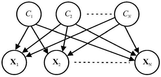
Figure 1.
Bayes’ theorem.
Applying the assumption that features are independent of each other yields
where . Since the denominator of Equation (2) is the same for all classes, comparing the numerator of it for each class is implemented in classifying features , . This comparison ends when Equations (3) and (4) are satisfied:
where denotes a class variable.
Regarding conventional sampling methods [7], this study designs user-based and item-based approaches in integrating Equations (3) and (4) with the selection of audit evidence:
- i.
- User-based approach: In an attempt to generate unbiased representations of data, classify and compute two percentile symmetric around the median of each class according to an auditor’s professional preferences. Draw the bounded by the resulting percentiles as audit evidence;
- ii.
- Item-based approach: Suppose the represent risky samples. Asymmetrically sample them based on the values as audit evidence after classifying .
3.1. User-Based Approach
Suppose the is a class after classifying . For implementing this classification, we compute posterior probabilities and regress the resulting values by a posterior probability distribution. Figure 2 shows an example. Deriving the detailed expression of this posterior probability distribution is unnecessary since deriving such an expression is not our goal. On the curve in Figure 2, we can determine two percentiles symmetric around the median. Draw samples bounded by the resulting percentiles audit evidence. In mathematical formulations, the present user-based approach implements the following Equation (5) to output audit evidence:
where and are two percentiles defining this confidence interval.
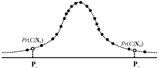
Figure 2.
Construction of a posterior probability distribution.
Auditors may have unique preferences of percentiles and . For example, if and are 97.5th and 2.5th percentiles, samples represent audit evidence in a 95% confidence interval.
Furthermore, computing posterior probabilities of samples yields
After drawing audit evidence, this study measures the representativeness of these by [6]
in which , is the total number of members in the class, and F is the cumulative distribution function of the curve in Figure 2. Since are discrete, this F function is equal to
where . If total members in the class are sampled, the representativeness index is identical to 1. On this value, the goal of drawing audit evidence may be choosing sufficient samples but maintaining high values.
Regarding existing audit sampling methods [7], the present user-based approach may be identical to a combination of the monetary and variable sampling methods.
3.2. Item-Based Approach
Similarly, manipulating Section 3.1, suppose is one of the classes resulting from the classification of data in which are members of this class.
If we have a null hypothesis that members of the class are risky, a member of this class with a lower value increases the possibility of rejecting this . Hence, drawing this as an audit evidence is valueless. To strengthen the belief that is true, it is better to asymmetrically sample members satisfying:
where and represents a selected threshold.
Furthermore, samples and may be simultaneously risky. Selecting them as audit evidence may be valuable. This selection may be based on the posterior probabilities of :
Further simplifying Equation (10) results in
Samples satisfying are drawn as audit evidence in which is another selected threshold. The upper bound of Equation (11) depends upon the value. To save time in searching those suitable for applying Equation (11), the Apriori algorithm states that we may start the search from those samples satisfying Equation (9). Such audit evidence may produce larger numerators in the last expression of Equation (11).
Furthermore, extending Equation (10) to samples yields
Samples satisfying are selected as audit evidence in which denotes third chosen threshold. Similarly, the upper bound of Equation (12) depends upon the value. Again, the Apriori algorithm suggests that we can choose samples from those satisfying .
Regarding existing audit sampling methods [7], the present item-based approach may be equivalent to a combination of non-statistical and monetary sampling methods.
Like Section 3.1, we calculate the representativeness index [6] to check whether audit evidence is sufficiently representative.
If the Python programming language is employed, one may use the Scikit-learn package to implement Equations (3) and (4). The classification results can be stored in an Excel file. We just program a few codes to implement Section 3.1 and Section 3.2. Teaching an auditor to create such codes is feasible.
3.3. Hybrid Approach
Auditors may hybridize the resulting works in Section 3.1 and Section 3.2 to balance representativeness and riskiness. We first apply the user-based approach to sample representative members bounded by two percentiles symmetric around the median of a class. Applying the item-based approach to sample asymmetrically risker samples is next performed among those resulting representative samples.
4. Results
This study generates three experiments to illustrate the benefits and limitations of combining a machine learning algorithm with sampling. The first experiment demonstrates that machine learning integration helps avoid sampling bias and maintains randomness and variability. The second experiment shows that the proposed works help sample unstructured data. The final experiment shows that the hybrid approach balances representativeness and riskiness in sampling audit evidence.
Referring to the previous study [15], implementing machine learning integration with sampling is better based on the accurate classification results provided by a machine learning algorithm. Therefore, this study chooses a random forest classifier and a support vector machines model with a radial basis function kernel as baseline models.
4.1. Experiment 1
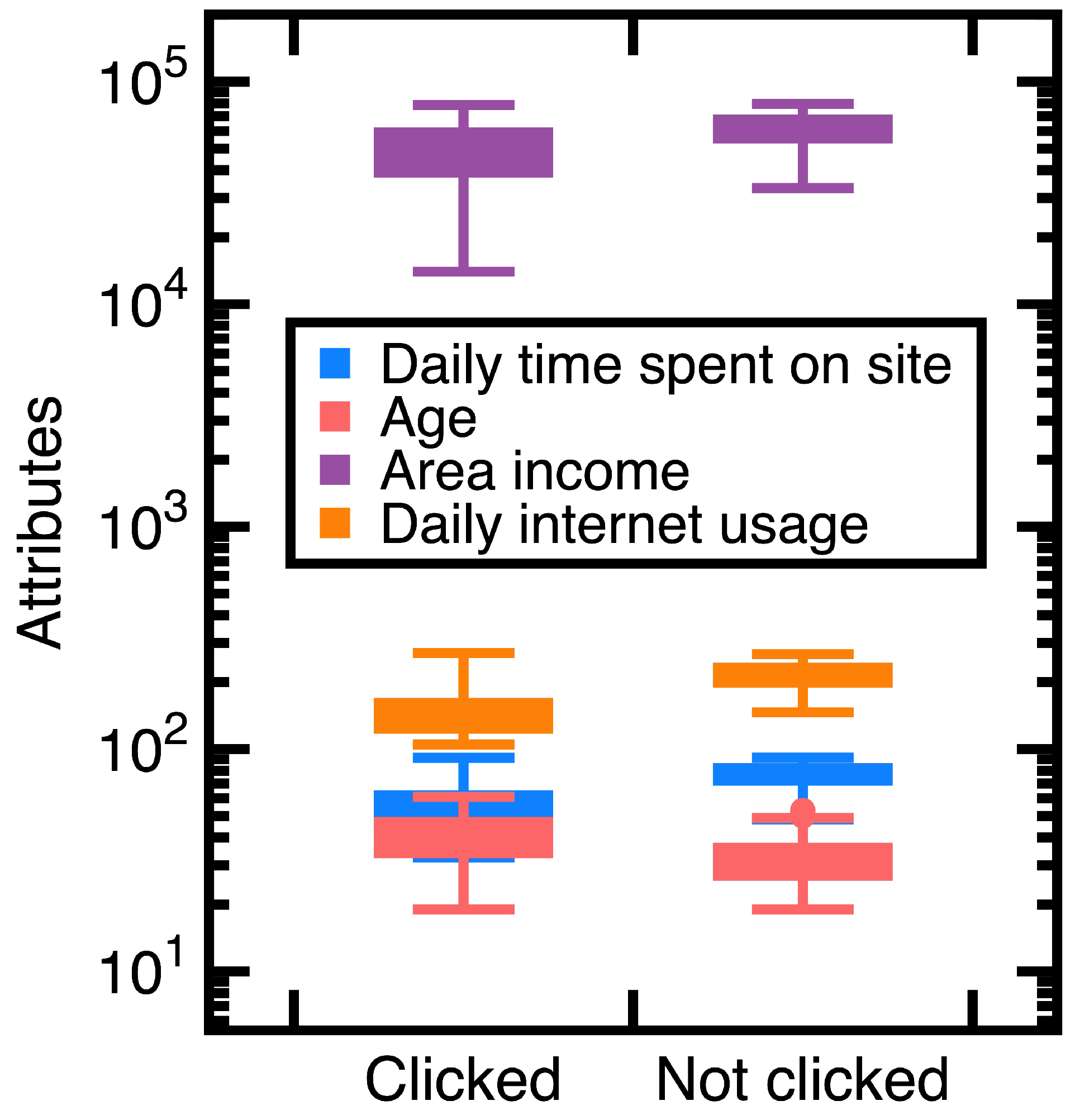
A customer ad click prediction data set contains (i.e., ) records in which 50% of customers clicked the advertisement and the remaining 50% did not. This study uses the ‘Daily time spent on site’, ‘Age’, ‘Area income’, ‘Daily internet usage’, and ‘Clicked on Ad’ columns as experimental data. Two-thirds of those records are randomly chosen as train data, whereas others are test data. The ‘Daily time spent on site’, ‘Age’, ‘Area income’, and ‘Daily internet usage’ columns are attributes . Moreover, set the class variable to indicate the ‘Clicked on Ad’ column equal to ‘Clicked’ or ‘Not clicked’. Figure 3 shows variations of those values.
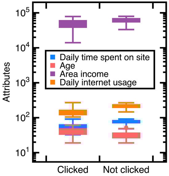
Figure 3.
Distributions of attributes ) values in Experiment 1.
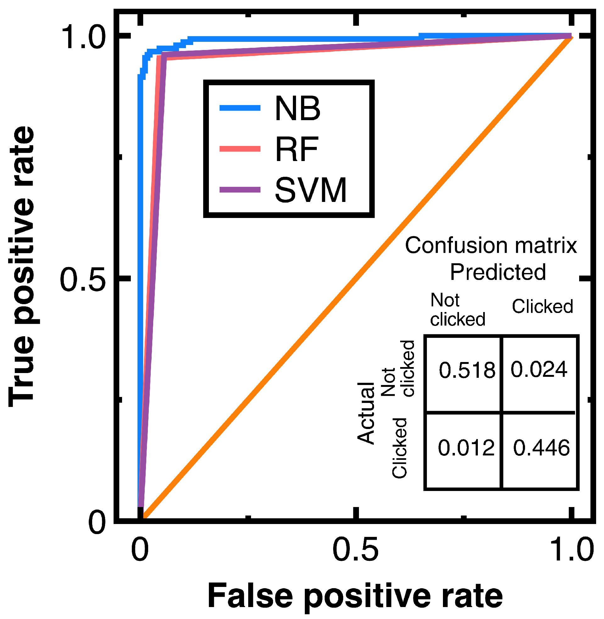
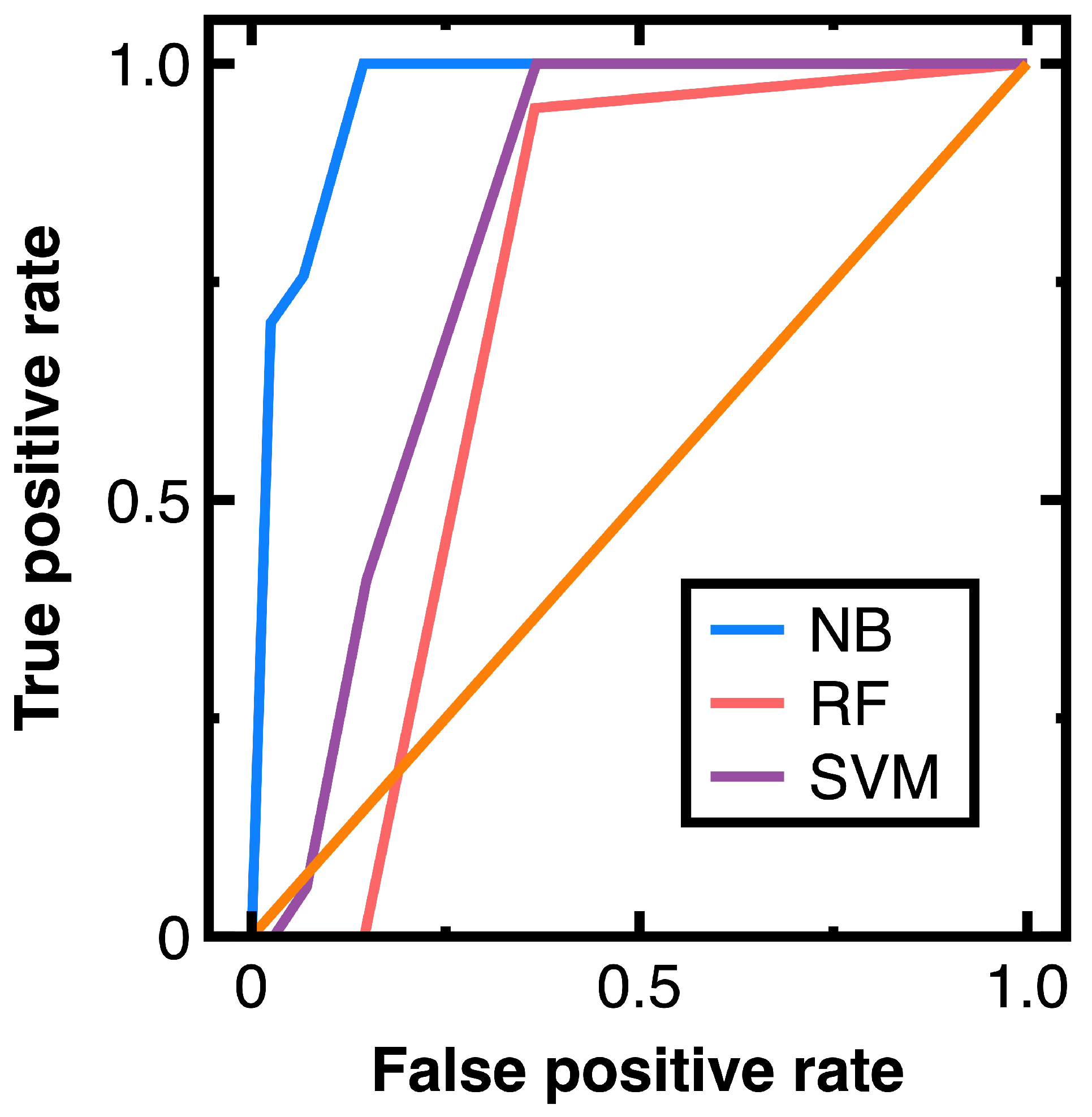
To avoid sampling frame errors [15], studying the classification accuracy output by Equations (3) and (4) is necessary. Figure 4 shows the resulting ROC curves in which NB, RF, and SVM are abbreviations of Naive Bayes, random forest, and support vector machines. This figure also shows the confusion matrix output by Equations (3) and (4). Its components have been normalized based on the amount of test data. Moreover, this study computes:

Figure 4.
ROC curves provided by different machine learning algorithms and the confusion matrix output by Equations (3) and (4) for Experiment 1.
Further computing the F1 score from Equations (14) and (15) yields
Meanwhile, calculating the AUC from Figure 4 obtains 0.965 (Equations (3) and (4)), 0.953 (a random forest classifier), and 0.955 (a support vector machines model with a radial basis function kernel). These AUC values indicate that Equations (3) and (4) slightly outperform the random forest classifier and support vector machines model with a radial basis function kernel in avoiding sampling frame errors and undercoverage. However, all three algorithms are good models.
Our aim for testing Section 3.1 is to sample an unbiased representation of experimental data with machine learning integration. Figure 5 shows the resulting audit evidence with a 50% confidence interval for each class. Histograms on this figure’s top and right sides compare the distributions of original customers and audit evidence. In this figure, light and heavy gray points denote experimental data, whereas red and blue colors mark audit evidence. The total number of blue and red points in Figure 5 equals 250, respectively. Substituting the resulting audit evidence into Equation (7) obtains the representativeness indices listed in the legend of Figure 5.
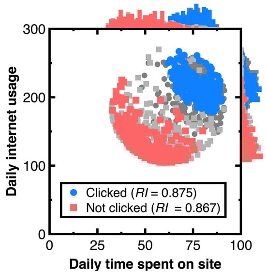
Figure 5.
Audit evidence for 50% confidence intervals.
Suppose the null hypothesis defines that the experimental data and audit evidence originate from the same probability distribution. We calculate the Kolmogorov–Smirnov test statistic [16] to quantify the possibility of rejecting this null hypothesis. The result is equal to 0.044, and it is less than the critical value equal to [16] for concluding Kolmogorov–Smirnov test statistics while considering the probability of 10% in rejecting the null hypothesize.
Calculating the Kolmogorov–Smirnov test statistic ensures that the audit evidence in Figure 5 is unbiased and representative of original customers. If the resulting Kolmogorov–Smirnov test statistic is lower than the critical value for concluding this test statistic, the original customers and audit evidence originate from the same probability distribution. Thus, we can reduce the risk of system errors or biases in estimating customers’ attributes.
We have another aim of keeping the variability in testing Section 3.2. As marked by a blue cross in Figure 6, choose a customer with the predicted posterior probability of 0.999. The caption of Figure 6 lists the attributes of this customer. Other customers relevant to this customer are drawn as audit evidence and marked using red points in Figure 6. Moreover, we still use light or heavy gray points representing the experimental data and histograms besides Figure 6 to describe the distribution of audit evidence. Since the denominator of Equation (11) equals 0.5, setting the threshold to 1.9999 is considered. Substituting the resulting audit evidence into Equation (7) yields the representativeness index in the legend of Figure 7. Counting the number of drawn audit evidence yields 294.
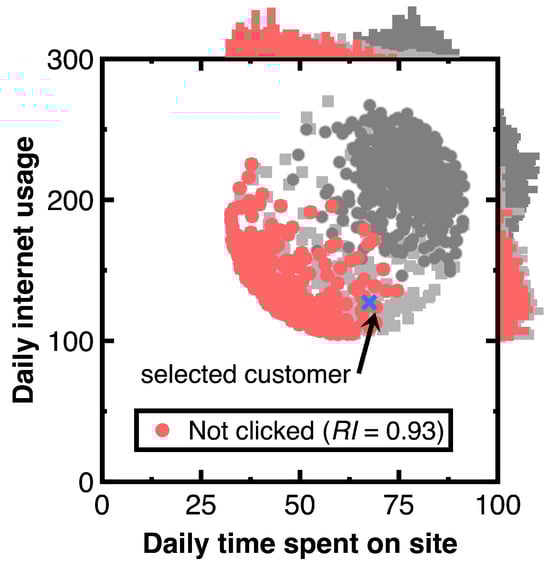
Figure 6.
Audit evidence relevant to a chosen customer (‘Daily time spent on site’ = 67.51, ‘Age’ = 43, ‘Area in-come’ = 23,942.61, ‘Daily internet usage’ = 127.2, and ‘Clicked on Ad’ = ‘Not clicked’).
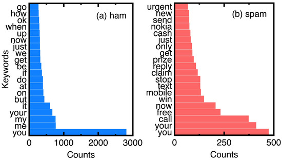
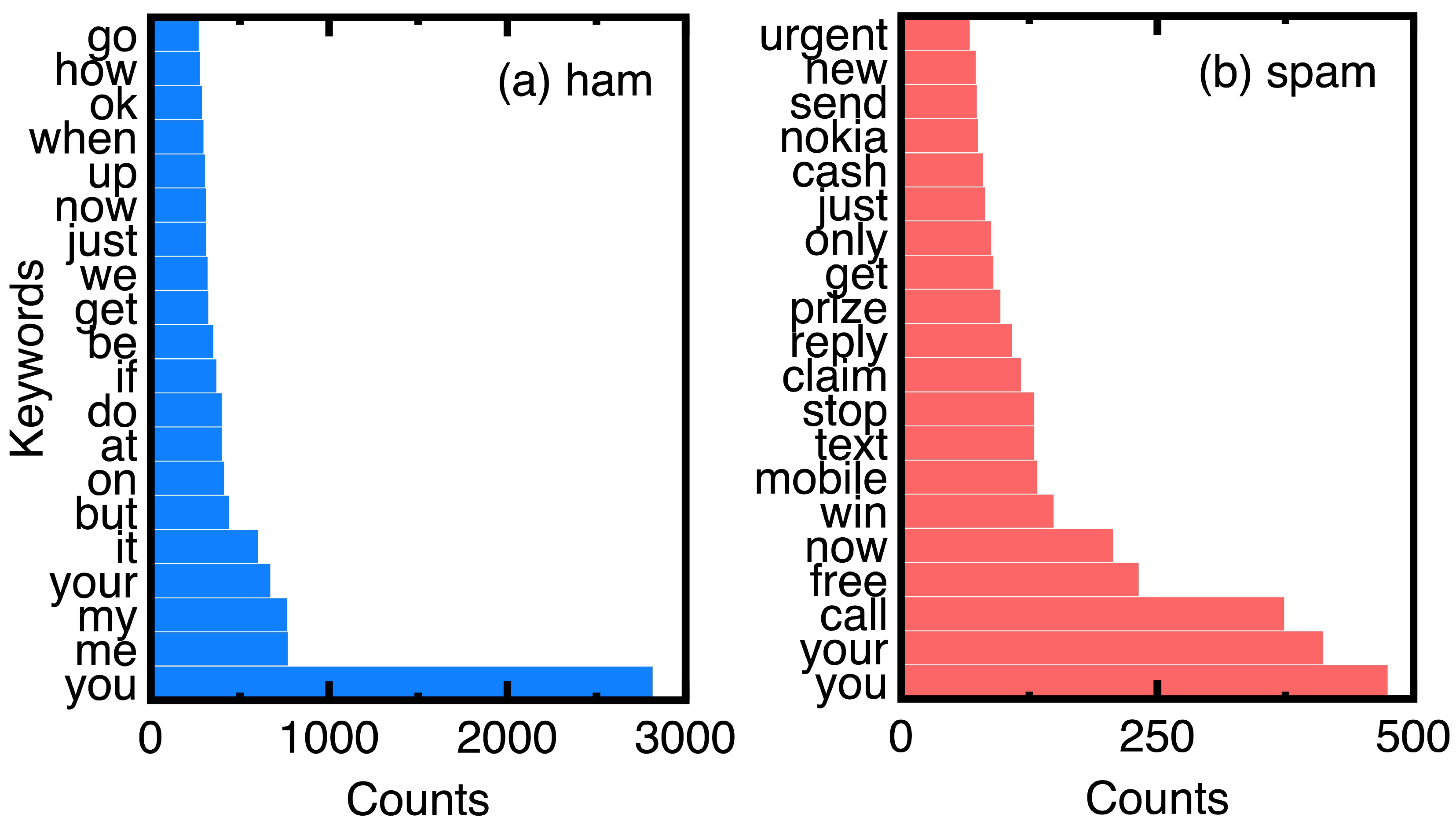
Figure 7.
Comparison of top 20 keywords in ham and spam messages: (a) ham messages; (b) spam messages.
Table 1 compares variability between the original ’Daily Internet use’ variable and audit evidence. We employ the range, standard deviation, interquartile range, and coefficient of variation to measure the variability.

Table 1.
Comparison of the variability between original customers and audit evidence.
Measuring the variability helps one understand the shape and spread of audit evidence. Table 1 shows that the audit evidence maintains the variability.
4.2. Experiment 2
A spam message is one of the unstructured data that did not appear in the conventional sampling. In this experiment, this study introduces a data set containing 5572 messages, and 13% of them are spam. This study randomly selects 75% of them as train data. The other 25% are test data. In implementing this experiment, the first step is preprocessing these train and test data by vectorizing each message into a series of keywords. We employ a dictionary to select candidate keywords. Counting their frequencies is next performed. Classifying ham and spam messages is done by setting a class variable indicating a spam or ham message, and attributes are the frequency of keywords.
Based on the counts of keywords in the ham and spam messages of experimental data, Figure 7 compares the top 20 keywords. Choosing them eliminates ordinary conjunctions and prepositions such as ’to’ and ’and.’ We can understand the unique keywords of spam messages from Figure 7.
To prevent sampling frame errors and undercoverage [15], Figure 8 compares the corresponding ROC curves versus different machine learning algorithms. It also shows the confusion matrix output by Equations (3) and (4). We have normalized its components based on the amount of test data. Table 2 lists other metrics for demonstrating classification accuracy on this confusion matrix.
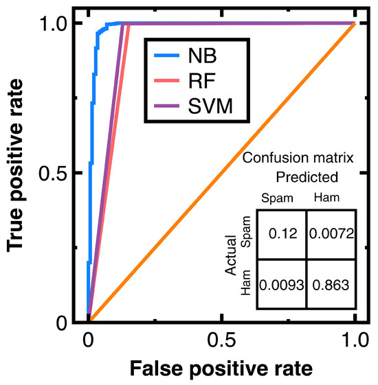
Figure 8.
ROC curves provided by different machine learning algorithms and the confusion matrix output by Equations (3) and (4) for Experiment 2.
Table 2.
Metrics output by Equations (3) and (4) for checking the classification accuracy for Experiment 2.
Calculating the AUC values from Figure 8 yields 0.989 (Equations (3) and (4)), 0.923 (random forest classifier), and 0.934 (a support vector machines model with a radial basis function kernel). Such AUC values indicate a support vector machines model and random forest classifier, and Equations (3) and (4) are all good models for preventing sampling frame errors and undercoverage; however, the performance of Equations (3) and (4) is still the best.
Next, this study chooses the 75% confidence interval of spam messages to generate audit evidence. We obtained 652 samples of spam messages. Figure 9 compares counts of the top 20 keywords of original text data and audit evidence. Substituting their posterior probabilities to compute the representativeness index equals 0.997.
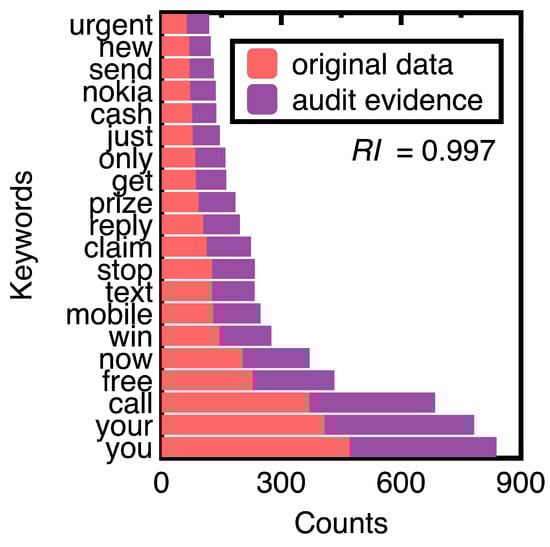
Figure 9.
Comparison of top 20 keywords in original text data and audit evidence.
Figure 9 demonstrates that machine learning integration promotes sampling unstructured data (e.g., spam messages) while keeping their crucial information. The design of conventional sampling methods does not consider unstructured data [7]. In this figure, sampling spam messages keeps the ranking of all the top 20 keywords. The resulting samples may form a benchmark data set for testing the performance of different spam message detection methods.
4.3. Experiment 3
The third experiment illustrates that integrating machine learning with sampling can balance representativeness and riskiness. We use the Panama Papers to create a directed graph model that has 535,891 vertices, in which each vertex denotes a suspicious financial account. Its attributes are the degree centrality and clustering coefficient.
The Panama Papers were a massive leak of documents. They exposed how wealthy individuals, politicians, and public figures worldwide used offshore financial accounts and shell companies to evade taxes, launder money, and engage in other illegal activities.
The degree centrality D [17] is the number of edges connecting to a vertex. The higher the degree centrality, the greater the possibility detects black money flows. Moreover, we consider that two financial accounts may have repeated money transfers. Therefore, computing the degree centrality considers the existence of multiple edges. For example, if a sender transfers money to a payee two times, the degree of a vertex simulating such a sender or payee equals 2.
Meanwhile, the clustering coefficient c [17] measures the degree to which nodes in a graph tend to group. Evidence shows that in real-world networks, vertices may create close groups characterized by a relatively high density of ties. In a money laundering problem, a unique clustering coefficient may highlight a group within which its members exchange black money. Like the computation of degree centrality, calculating the clustering coefficient considers the possible existence of multiple edges.
The purpose of generating Experiment 3 is to demonstrate that integrating machine learning with sampling can balance representativeness and riskiness. Therefore, we set the variable according to the and values. Table 3 lists the results. Its final column lists the total members corresponding to each class.
Table 3.
The resulting degree centrality , clustering coefficient , and total number of members in each class.
To prevent sampling frame errors and undercoverage [15], Figure 10 compares the ROC curves output by different machine learning algorithms in classifying nodes in Experiment 3. In Figure 10, 80% of random nodes are chosen as train data and other vertices are chosen as test data. Moreover, Equations (3) and (4) output the confusion matrix shown in Equation (18):
in which each component has been normalized based on the amount of test data.
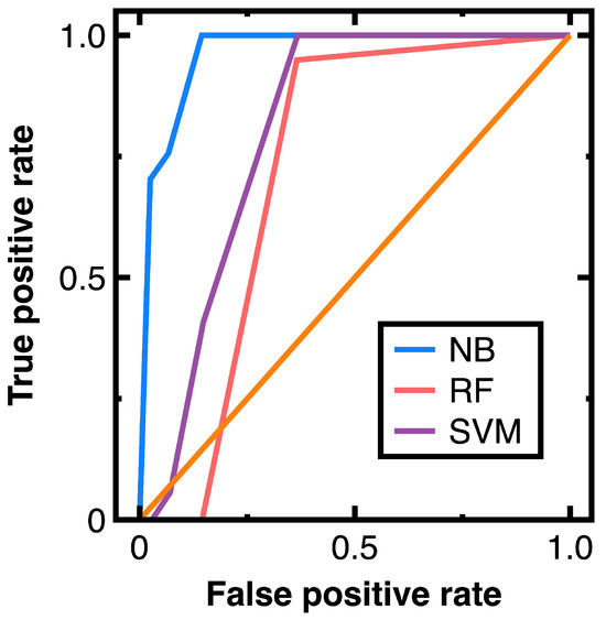
Figure 10.
ROC curves provided by different machine learning algorithms for Experiment 3.
From Equation (18), we further calculate the averaged accuracy, specificity, recall, precision, and F1 value, as shown in Table 4. Next, calculating the AUC values from Figure 10 and Table 4 results in 0.965 (Equations (3) and (4)), 0.844 (random forest classifier), and 0.866 (support vector machines model with a radial basis function kernel). Figure 10 indicates that the random forest classifier and support vector machines model with a radial basis function kernel are unsuitable for this experiment. Since we have a high volume of data in this experiment, these two algorithms may output unacceptable errors in sampling nodes.
Table 4.
Metrics calculated from Equation (18).
Suppose a 75% confidence interval to sample members of each class . However, we agree that the class has the risker members. High values imply frequent transactions. Therefore, further drawing audit evidence from samples with values within the 75% confidence interval of the class. The red points in Figure 11 represent the resulting audit evidence. Heavy gray points denote original data. The legend of this figure lists the corresponding representativeness index and the number of drawn samples.
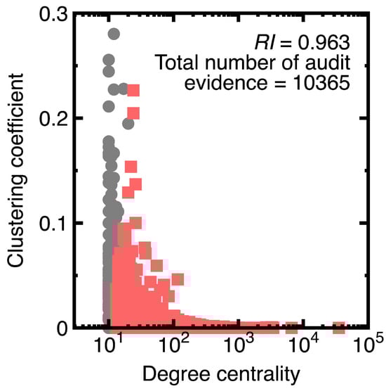
Figure 11.
Risker audit evidence for Experiment 3.
Carefully inspecting Figure 11 indicates that vertices () are drawn as audit evidence. They are riskier than other nodes in the class. With the help of a Naive Bayes classifier (Equations (3) and (4)), profiling the class is unnecessary before sampling this class. This unnecessity illustrates the difference between sampling with machine learning integration and conventional sampling methods.
5. Discussion
Section 4 implies the benefits and limitations of integrating a Naive Bayes classifier with sampling. We further list these benefits and limitations:
- Conventional sampling methods [7] may not profile the full diversity of data; thus, they may provide biased samples. Since this study samples data after classifying them using a Naive Bayes classifier, it substitutes for a sampling method to profile the full diversity of data. The experimental results of Section 4 indicate that the Naive Bayes classifier classifies three open data sets accurately, even if they are excessive. Those accurate classification results indicate that we capture the full diversity of the experimental data.
- Developing conventional sampling methods may not consider complex patterns or correlations in data [7]. In this study, we handle complex correlations or patterns in data (for example, a graph structure in Section 4.3) using a Naive Bayes classifier. This design mitigates the sampling bias caused by complex patterns or correlations if it provides accurate classification results.
- Section 4.3 indicates that a Naive Bayes classifier works well for big data in a money laundering problem. It outperforms the random forest classifier and support vector machines model with a radial basis function kernel in classifying massive vertices. Thus, we illustrate that the efficiency of sampling big data can be improved. One can sample risker nodes modeling fraudulent financial accounts without profiling specific groups of nodes.
- The development of conventional sampling methods considers structured data; however, they struggled to handle unstructured data such as spam messages in Section 4.2. We resolve this difficulty by employing a Naive Bayes classifier before sampling.
- Since this study samples data from each class classified by a Naive Bayes classifier, accurate classification results eliminate sample frame errors and improper sampling sizes.
- Although the source of this study is Taiwan’s auditors’ unsatisfactory workplace environment, our resulting works are applicable to auditors in other nations.
Nevertheless, this study also finds limitations in integrating machine learning and sampling. They are listed as follows:
- It is still possible that a Naive Bayes classifier provides inaccurate classification results. One should test the classification accuracy before sampling with machine learning integration.
- In implementing Section 3.2, thresholds are needed. However, we should inspect variations of the prior probabilities for determining proper values. They denote the second limitation of our machine-learning-based sampling.
6. Conclusions
Sampling plays a crucial role in auditing. It provides a mechanism for auditors to draw audit evidence. However, various challenges exist within available sampling methodologies, including selection bias, sampling frame errors, improper sampling sizes, and the handling of unstructured and massive data. This study develops a Naive Bayes classifier as a sampling tool for drawing data within a confidence interval symmetric to the median or sampling asymmetrically riskier samples. It is employed to overcome the challenges mentioned above. Auditors can build such a Naive Bayes if they have learned ordinary functions of the Python programming language.
From Section 4, we conclude:
- A Naive Bayes classifier is a more suitable classification algorithm for implementing the sampling with machine learning integration. It calculates posterior probabilities for the classification. These posterior probabilities are perfectly suitable as attributes in sampling.
- Sampling with machine learning integration has the benefits of providing unbiased samples, handling complex patterns or correlations in data, processing unstructured or big data, and avoiding sampling frame errors or improper sampling sizes.
- An ordinary Naive Bayes classifier is sufficient as a ’Black Box’ for sampling data. Implementing a Naive Bayes classifier to sample excessive data can be completed by a few auditors.
- The first step of sampling unstructured data can be classifying these unstructured data. Sampling classification results is the next step.
- Machine learning can help reduce human expenses. It mitigates the need for more young auditors. With the introduction of machine learning algorithms, enterprises require few auditors.
However, sampling using a Naive Bayes classifier has limitations. Inaccurate classification results output by the Naive Bayes classifier may result in biased samples or sampling frame errors. Overcoming them requires testing the Naive Bayes classifier before applying it to sampling. Precalculating the range of posterior probabilities is also necessary for choosing specific samples. Fortunately, such calculation is necessary to implement a Naive Bayes classifier.
Author Contributions
Conceptualization, G.-Y.S.; methodology, G.-Y.S.; software, G.-Y.S.; validation, N.-R.L.; formal analysis, G.-Y.S.; investigation, G.-Y.S.; resources, G.-Y.S.; data curation, N.-R.L.; writing—original draft preparation, N.-R.L.; writing—review and editing, G.-Y.S.; visualization, N.-R.L.; supervision, G.-Y.S.; project administration, G.-Y.S.; and funding acquisition, N.-R.L. All authors have read and agreed to the published version of the manuscript.
Funding
The research was funded by the National Science and Technology Council, R.O.C., grant number: 112-2813-C-309-002-H.
Data Availability Statement
Customer ad click prediction dataset at https://www.kaggle.com/code/mafrojaakter/customer-ad-click-prediction (accessed on 15 December 2023); SMS spam collection dataset at https://www.kaggle.com/code/mafrojaakter/customer-ad-click-prediction (accessed on 15 December 2023); Panama Papers at https://offshoreleaks.icij.org/pages/database (accessed on 15 December 2023).
Conflicts of Interest
The authors declare no conflicts of interest.
References
- Deng, H.; Sun, Y.; Chang, Y.; Han, J. Probabilistic Models for Classification. In Data Classification: Algorithms and Applications; Aggarwal, C.C., Ed.; Chapman and Hall/CRC: New York, NY, USA, 2014; pp. 65–86. [Google Scholar]
- Schreyer, M.; Gierbl, A.; Ruud, T.F.; Borth, D. Artificial intelligence enabled audit sampling— Learning to draw representative and interpretable audit samples from large-scale journal entry data. Expert Focus 2022, 4, 106–112. [Google Scholar]
- Zhang, Y.; Trubey, P. Machine learning and sampling scheme: An empirical study of money laundering detection. Comput. Econ. 2019, 54, 1043–1063. [Google Scholar] [CrossRef]
- Aitkazinov, A. The role of artificial intelligence in auditing: Opportunities and challenges. Int. J. Res. Eng. Sci. Manag. 2023, 6, 117–119. [Google Scholar]
- Chen, Y.; Wu, Z.; Yan, H. A full population auditing method based on machine learning. Sustainability 2022, 14, 17008. [Google Scholar] [CrossRef]
- Bertino, S. A measure of representativeness of a sample for inferential purposes. Int. Stat. Rev. 2006, 74, 149–159. [Google Scholar] [CrossRef]
- Guy, D.M.; Carmichael, D.R.; Whittington, O.R. Audit Sampling: An Introduction to Statistical Sampling in Auditing, 5th ed.; John Wiley & Sons: New York, NY, USA, 2001. [Google Scholar]
- Schreyer, M.; Sattarov, T.; Borth, D. Multi-view contrastive self-supervised learning of accounting data representations for downstream audit tasks. In Proceedings of the Second ACM International Conference on AI in Finance Virtual Event, New York, NY, USA, 3–5 November 2021. [Google Scholar] [CrossRef]
- Schreyer, M.; Sattarov, T.; Reimer, G.B.; Borth, D. Learning sampling in financial statement audits using vector quantised autoencoder. arXiv 2020, arXiv:2008.02528. [Google Scholar]
- Lee, C. Deep learning-based detection of tax frauds: An application to property acquisition tax. Data Technol. Appl. 2022, 56, 329–341. [Google Scholar] [CrossRef]
- Chen, Z.; Li, C.; Sun, W. Bitcoin price prediction using machine learning: An approach to sample dimensional engineering. J. Comput. Appl. Math. 2020, 365, 112395. [Google Scholar] [CrossRef]
- Liberty, E.; Lang, K.; Shmakov, K. Stratified sampling meets machine learning. In Proceedings of the 33rd International Conference on Machine Learning, New York, NY, USA, 19–24 June 2016. [Google Scholar]
- Hollingsworth, J.; Ratz, P.; Tanedo, P.; Whiteson, D. Efficient sampling of constrained high-dimensional theoretical spaces with machine learning. Eur. Phys. J. C 2021, 81, 1138. [Google Scholar] [CrossRef]
- Artrith, N.; Urban, A.; Ceder, G. Constructing first-principles diagrams of amorphous LixSi using machine-learning-assisted sampling with an evolutionary algorithm. J. Chem. Phys. 2018, 148, 241711. [Google Scholar] [CrossRef] [PubMed]
- Huang, F.; No, W.G.; Vasarhelyi, M.A.; Yan, Z. Audit data analytics, machine learning, and full population testing. J. Financ. Data Sci. 2022, 8, 138–144. [Google Scholar] [CrossRef]
- Kolmogorov, A. Sulla determination empirica di una legge di distribuzione. G. Inst. Ital. Attuari. 1933, 4, 83–91. [Google Scholar]
- Wasserman, S.; Faust, K. Social Network Analysis: Methods and Applications, 1st ed.; Cambridge University Press: Cambridge, NY, USA, 1994. [Google Scholar]


Disclaimer/Publisher’s Note: The statements, opinions and data contained in all publications are solely those of the individual author(s) and contributor(s) and not of MDPI and/or the editor(s). MDPI and/or the editor(s) disclaim responsibility for any injury to people or property resulting from any ideas, methods, instructions or products referred to in the content. |
© 2024 by the authors. Licensee MDPI, Basel, Switzerland. This article is an open access article distributed under the terms and conditions of the Creative Commons Attribution (CC BY) license (https://creativecommons.org/licenses/by/4.0/).