Abstract
Autonomy of breast cancer classification is a challenging problem, and early diagnosis is highly important. Histopathology images provide microscopic-level details of tissue samples and play a crucial role in the accurate diagnosis and classification of breast cancer. Moreover, advancements in deep learning play an essential role in early cancer diagnosis. However, existing techniques involve unique models for each classification based on the magnification factor and require training numerous models or using a hierarchical approach combining multiple models irrespective of the focus of the cell features. This may lead to lower performance for multiclass categorization. This paper adopts the DenseNet161 network by adding a learnable residual layer. The learnable residual layer enhances the features, providing low-level information. In addition, residual features are obtained from the convolution features of the preceding layer, which ensures that the future size is consistent with the number of channels in DenseNet’s layer. The concatenation of spatial features with residual features helps better learn texture classification without the need for an additional texture feature extraction module. The model was validated for both binary and multiclass categorization of malignant images. The proposed model’s classification accuracy ranges from 94.65% to 100% for binary and multiclass classification, and the error rate is 2.78%. Overall, the suggested model has the potential to improve the survival of breast cancer patients by allowing precise diagnosis and therapy.
1. Introduction
Breast cancer is a widespread disease affecting millions of women worldwide. Early detection and diagnosis of breast cancer can significantly improve the chances of successful treatment and patient survival. Medical imaging is one of the primary methods used for diagnosing breast cancer. The most common techniques are as follows.
- Mammography: Mammography is an X-ray imaging technique used to examine breast tissue.
- Ultrasound: Ultrasound imaging uses high-frequency sound waves to produce images of the breast tissue.
- Magnetic resonance imaging (MRI): MRI is a noninvasive imaging technique that uses powerful magnetic fields and radio waves to produce detailed images of breast tissue.
- Histopathological images: Histopathological images involve examining tissue samples from a patient’s breast to identify the presence of cancerous cells.
Histopathological images are preferable for breast cancer detection over other imaging techniques because they provide high-resolution images of tissue samples obtained from the breast. These images allow pathologists to examine tissue at the cellular level and identify the presence of cancerous cells. In contrast, mammography, ultrasound, and MRI are imaging techniques that provide images of the breast tissue as a whole and can detect abnormalities in the tissue, but they cannot definitively diagnose cancer [1]. Further testing, such as a biopsy, is typically required to confirm the presence of cancer. Pathologists can examine the size, shape, and characteristics of cancerous cells and determine the stage and grade of cancer, which is important for determining the appropriate treatment plan. Additionally, histopathological images can be used to analyze biomarkers, such as hormone receptor status and HER2/neu expression, which can provide important information about cancer and help guide treatment decisions [2]. Overall, histopathological images are a crucial tool in the diagnosis and treatment of breast cancer, and they provide a more comprehensive assessment of cancerous tissue than other imaging techniques.
The analysis of histopathological images is a challenging task that requires significant expertise and experience from the pathologist. Deep-learning algorithms can be trained on large datasets of histopathological images to classify breast tissue as either cancerous or noncancerous. These algorithms can learn to identify features such as the shape, size, and texture of cancerous cells and clusters of cells, which can indicate breast cancer. The use of deep-learning-based breast cancer classification on histopathological images has the potential to improve the accuracy and speed of breast cancer diagnosis, leading to earlier detection and better patient outcomes. Moreover, pathologists can assist in the interpretation of histopathological images, potentially reducing the burden on healthcare systems and improving patient care. Although deep-learning models are efficient at performing image classification, their spatial features are sensitive to shape and position. Thus, classifying histopathological images with texture patterns using spatial feature-oriented deep CNNs is inefficient.
Deep learning allows for the exploration of symmetry in data and models. When training a machine learning model, it might be challenging, if not impossible, to get the weights to vary if they are all initially set to the same value. The "symmetry" happens here. By setting the model’s initial values to tiny, arbitrary numbers, we can disrupt the symmetry and let the various weights learn separately. Liu et al. [3] demonstrated the significance of orderless encoding for texture pattern representation. Zhang et al. [4] integrated Fisher vector encoding with a pretrained CNN model for texture classification. However, the benefits of end-to-end learning are not completely leveraged because the methods suggested in [4] require many phases, including feature extraction, orderless encoding, and dimension reduction. Furthermore, all these approaches operate on large matrices due to the high dimensionality of the features they extract. For effective feature transfer for pattern recognition, a complete learning approach that incorporates the residual pooling layer into any pretrained CNN model was proposed in [5]. This paper aims to classify cancerous histopathological images using this approach. The strength of the encoding in the CNN layers is targeted in the proposed structure to use spatial and spectral features, improving the overall classification accuracy. In the proposed method, residual layer-based encoding and concatenation of features from the previous layers are performed to make the method a learnable layer and to reduce the feature size. The DenseNet161 network is adopted, and learnable residual pooling layers are added for encoding and dimension reduction to learn from the texture features. The overall contributions of the paper are as follows:
- A residual feature that represents spatial features from the present layers is integrated with the spatial features of previous layers. The retention of residual features before integrating them with the features of previous layers helps us better learn texture classification [5].
- A complete framework integrating learnable residual features with a pretrained DenseNet161 network is presented for histopathological image classification. An experimental evaluation using binary classification and multiclass classification is presented.
- A state-of-the-art comparison with other residual and CNN networks classifying benign and malignant images and malignant image subclass categorization for the benchmark dataset used is presented.
The remainder of the paper is structured as follows: An overview of residual network-related work and histopathological image classification using a deep CNN are presented in Section 2. Section 3 describes the proposed network and its layer structure. The experimental results, discussion, and comparative analysis are presented in Section 4. The conclusion is presented in Section 5.
2. Related Work
CNNs are effective in approximating functions for a wide range of tasks and have shown successful results in different fields. Increasing the number of layers in a CNN can help improve its accuracy, but there is a limit to how many layers can be added before the accuracy starts to decrease. Traditional CNNs can also suffer from issues such as loss of spatial features and decreased accuracy for deep networks, as well as large learnable parameter counts that can make training difficult. To overcome these challenges, an integrated approach that combines different techniques may be necessary. Prushty et al. presented a comparison of machine-learning models on four diagnosis approaches, including Schiller, Hinselmann, cytology, and biopsy [6]. The random forest outperformed all traditional machine-learning approaches.
A transformer-based architecture, i.e., the ScoreNet network, was designed for histopathological image classification [7]. By leveraging local and global attention mechanisms, ScoreNet extracts features at both the cell and tissue levels. Moreover, a novel data augmentation technique called ScoreMix is introduced, which generates coherent sample-label pairs based on the semantic distribution of the image. ScoreNet achieves state-of-the-art results on the BRACS dataset and demonstrates high efficiency compared to other transformer-based architectures, such as TransPath and the Swin Transformer. A ResNet152 network was used to detect whether an image was cancerous by Gandomkar et al. [8]. ResNet was trained individually for each magnification factor, and a decision tree was subsequently constructed by combining the outcomes of all the trained networks to determine whether the image was malignant. In reference [9], the authors proposed an optimization of the DenseNet architecture and experimental accuracy for binary classification with a 99% classification rate using the BreakHis dataset. However, the classification rate at each magnification factor and multiclass classification were not evaluated. The optimization and fine-tuning of the DenseNet network using fast AI and one cycle are presented in [10]. This optimized network was used to classify the positive and negative samples from the BreakHis datasets, achieving an accuracy of 92%.
Texture features play a vital role in enhancing multiclass classification accuracy. The wavelet transform provides a multiresolution framework that can extract structural information well. Wavelet transforms providing both spatial and spectral information were integrated with convolution features by Mewada et al. [11] and validated using the BCC2015 dataset with an accuracy of 97%. Liu et al. observed that histopathological images generated using an optical microscope contain noise that may impact CNN classification. Therefore, an adaptive thresholding-based wavelet transformation was adopted with CNN for denoising during the network training. Their model received 94.37% binary classification on the BreakHis dataset [12]. In [13], authors preprocessed images for noise removal and enhancement using weighted guided filtering and Gamma correction. Later, a hierarchical approach was presented to extract optimal structural features using superpixel mixed clustering, GLCM, and optimization algorithms. Finally, features were used to train a dense capsule network for the classification.
Histopathological images have many features because of the presence of texture regions. Dictionary-based sparse representation can increase the discrimination capability of algorithms [14]; therefore, a class-level dictionary-based classification model was presented in [15], and a validated model with a 93.33% binary classification rate was used. Another deep-learning strategy based on the FE-BkCapsNet model was developed by Wang et al. [16]. This method merged the CNN model (which focuses on semantics) and the CapsNet model (which focuses on spatial characteristics). The success rate ranged between 92.71% and 94.52% for image categorization in the BreakHis dataset. However, to produce correct results, these CNN models employ many convolutional layers and parameters, which consumes computer resources and time. Pandey et al. [17] developed three distinct models for binary, benign, and malignant category classifications. In the first phase, the model separates benign from malignant images. This method is repeated for all magnification factors separately, resulting in the training and validation of 12 unique models. The authors employed a pretrained Xception [18] model with classification layers added according to the categorization at hand.
To reduce the complexity of the CNN, a convolution autoencoder was proposed and trained from scratch using the BreakHis dataset [19]. However, the model accuracy, precision, and recall rate are limited to 84.72%, 86.87%, and 80.23%, respectively. A squeeze-and-excitation block was integrated with the residual layer of ResNet, reducing the size of the network by 33% at the cost of accuracy for multiclass classification [20]. Their model performed well for binary classification at all magnification levels, with a maximum accuracy of 99.34% at the 200X level. This model achieved accuracies ranging between 90.66% and 93.81% for multiclass classification. A similar hybrid architecture using ResNet18 and a squeeze-and-excitation block was presented by Liu et al., who focused on minimizing the difference in distribution between labeled and unlabeled samples [21]. They validated their model for eight-class classification, achieving 93.24% accuracy. A tiny swin transformer that operates on nonoverlapping patches of images was used with a SoftMax classifier at the end for eight-class classification [22]. However, a smaller model size impacts complex pattern handling and may impact the model capacity. A complex hierarchical model was presented in [23], where an SVM was initially used to screen image patch labels, i.e., benign patches obtained from malignant images; subsequently, these labeled images were used to train the resolution adaptive network. SURF features were used in the SVM classifier to label the patches from the images. The model achieved 91.14% accuracy for multiclass classification, and there is a need to improve the classification accuracy at the 400X magnification level.
The preceding study emphasized the significance of employing pretrained models and data augmentation strategies to improve model performance. However, traditional CNNs may suffer from issues such as loss of spatial features, decreased accuracy for deep networks, and large learnable parameter counts that can make training difficult. Hybrid approaches with many layers in CNN may enhance classification at the cost of increased resources and time consumption. In addition, the performance of some models varies depending on the magnification factor used. Although most models classify malignant and benign images well, there is room for improvement in the use of the multiclass model for categorizing malignant images. The next section presents the proposed network, which aims to address the multiclass classification problem by adding texture information with spatial information without the need for an additional algorithm. Furthermore, a straightforward yet efficient integrated approach allows for the classification of breast cancer histopathology at multiple levels within a single model.
3. Proposed Method
Histopathology images, used for diagnosing and studying diseases at the cellular level, contain various texture regions. These textures can hold important information for classifying and analyzing images. While the global convolutional features of a CNN can capture overall patterns and structures in an image, they may not be sufficient to capture the local variations and repetitions of patterns that are characteristic of different textures. To accurately classify histopathology images, a tactful approach that combines both local and global information fusion is needed. This integration of both local and global information allows for a comprehensive understanding of the image, considering both the fine details within specific regions and the overall context of the image. A learnable residual approach is adopted in the proposed network to extract the local features, and spatial features are subsequently integrated with residual features for classification. The proposed model is as follows:
3.1. Residual Feature Extraction
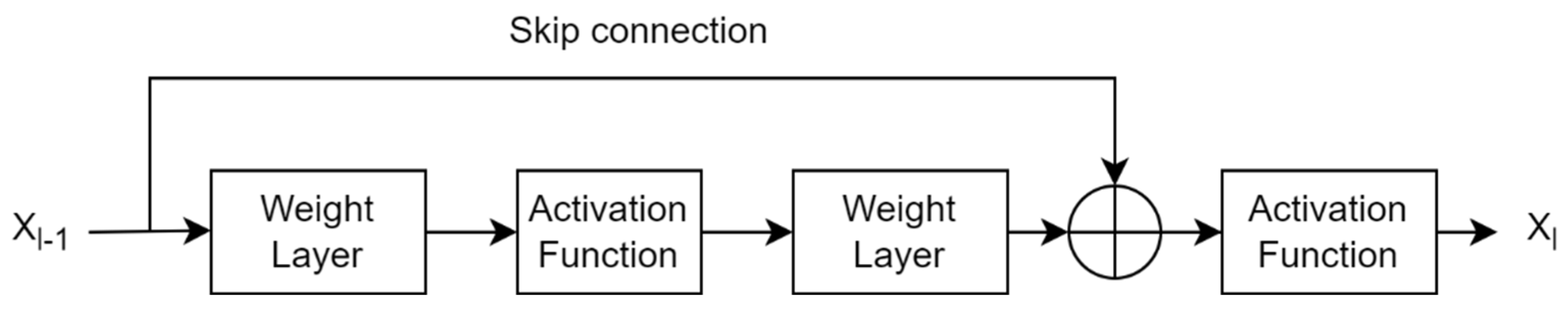
A traditional CNN uses pretrained layers and trainable convolutional layers to extract spatial features from the image plane. These layers provide global (or spatial) features, ignoring local (or spectral) features. Since texture image classification requires local patterns, traditional CNNs do not perform well in texture pattern classification. There is a need to pass texture-specific features to the classification layer while still maintaining global features because they are effective at identifying texture patterns. This architecture configuration allows for completely connected layers with useful texture features and aids in more accurate class boundary estimation. Global average pooling eliminates dependency on spatial location by averaging all features and can add robustness to spatial features obtained from traditional CNN layers [24]. However, simple averaging features completely ignore features’ spatial layout, resulting in inefficient encoding of discrimination features. An alternative approach is a multistep model that employs global feature extraction, local feature extraction (i.e., orderless encoding), and dimension reduction models simultaneously for classification. A similar approach was presented in [5] using texture encoding model integration in a residual network. A residual block learns from the difference in the features of two consecutive layer blocks in the residual network. This traditional residual block is shown in Figure 1.

Figure 1.
Traditional formation of a residual layer in a convolutional neural network.
If x represents the features obtained from the previous layer of the CNN, Xl gives the output features if Xl−1 passes through the current layers l of the CNN with weights of Wl−1 = {Wl−1, k}, it can be expressed as
where 1< k < K gives the number of layers in one unit, represents a residual function that captures the desired transformation of the input. Then, the residual feature can be expressed as
The skip connection has a larger gradient. Therefore, the residual layer also helps in minimizing the vanishing gradient problem during backpropagation due to its skip connection. ResNet is a popular deep network that provides residual features. However, the interpretability of these features is limited because skip connections do not interpret meaningful information as nontrainable connections.
The primary objective is to extract and use local features in addition to global features. In the proposed method, a pretrained DenseNet161 architecture is modified by adding the proposed residual layers after the last convolutional layer. The spatial features obtained from the final convolutional layer of the DenseNet161 network are used to compute the residual. In the proposed residual layer, a skip connection is adopted with a kernel size of 1 × 1, stride of 1, and sigmoid activation function, as explained in [5]. The role of the kernel (K) in the skip connection is to provide new learning features from the pretrained features at each pixel location in the image, and its size is similar to the input. Later, the sigmoid function (σ) emphasizes the difference between the newly learned features and pretrained features. Thus, residual features providing local information can be calculated as
Thus, the adopted skip connection provides learnable features for each pixel. The dropout and batch normalization in this connection help to solve the problem of overfitting. This structure is shown in Figure 2.
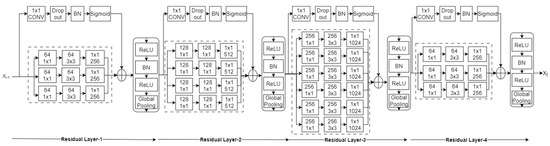
Figure 2.
Learnable residual layer-based deep CNN.
As explained, global average pooling is mostly used to obtain robustness to spatial position in global features. In the adopted network, ReLU is used to force negative residual features to zero, followed by batch normalization and global average pooling, which aggregate features, restricting the dimension of features to the number of channels in the pretrained network’s last convolutional layer. Thus, it protects the extension of feature dimensions in contrast to Fisher vector-oriented CNNs [24] and deep-ten networks [4].
3.2. Concatenation of Global Spatial Features and Residual Features
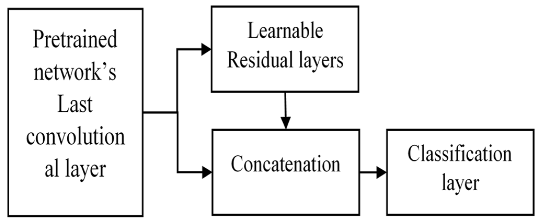
The convolutional features are obtained from the pretrained DenseNet161 layers, which represent global features. These features act as inputs for learnable residual layers, as shown in Figure 2, which serve as local features at each pixel in the image plane. We concatenated these residual features with global features. The concatenation serves the purpose of obtaining both local and global feature requirements to classify the texture patterns in histopathological images. The overall structure is as follows (Figure 3).
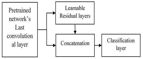
Figure 3.
Proposed extended deep network using learnable residual layers for image classification.
This extension is versatile and applicable to any image size since the initial layers are DenseNet layers. The learnable residual layers give fixed-dimensional features for arbitrary image sizes. Thus, for larger images, more detailed local information can be fetched using this architecture.
4. Results and Discussion
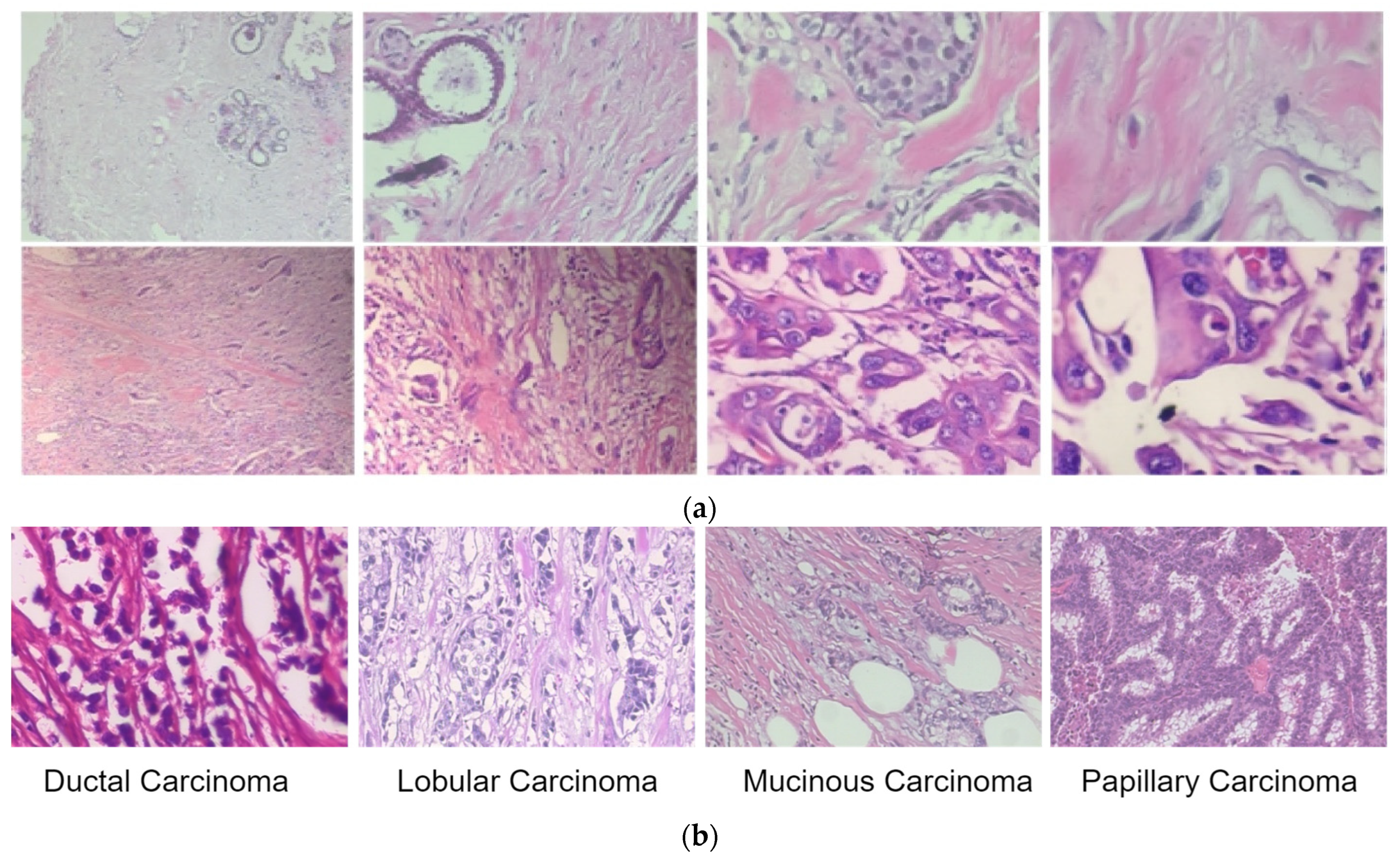
We used the proposed extension of the DenseNet network for breast cancer classification using histopathological images. The publicly available BreakHis dataset [25] consists of benign and malignant classes, and magnification factors of 40X, 100X, 200X and 400X are used to test and validate the network. Overall, there are 7909 images in the BreakHis dataset, including 2480 benign types and 5429 malignant types, each with 700 × 460 resolution. The malignant images were further classified as ductal carcinoma (DC), lobular carcinoma (LC), mucinous carcinoma (MC), or papillary carcinoma (PC). The sample images from the BreakHis dataset are shown in Figure 4.

Figure 4.
Sample images of benign and malignant lesions from the BreakHis dataset. (a) Benign (first row) and malignant images (in the second row) at four magnification levels of 40X, 100X, 200X and 400X (left to right). (b) Sample images of malignant lesion classes.
Table 1 shows the distribution of images according to their class. The proposed model is validated in two phases. First, the model is tested for binary classification; second, it is tested for multiclass classification for malignant images. To obtain local and global features efficiently, these large images are divided into 512 × 512 patches. To increase the size of the datasets, augmentation is applied to each patch via rotation, mirroring, and shifting operations. The histopathological images have different color channels; therefore, the mean value of each color channel is subtracted for each channel individually to normalize each patch, after which rotation and vertical mirroring are applied to each patch during the augmentation process. This augmentation can help to overcome the overfitting problem in the training stage. In data loading, it is configured such that it randomly shuffles the data samples each time a new epoch starts. This randomization helps in reducing any potential bias or overfitting that may arise from the order of the samples. The model’s performance is evaluated on unseen data that is independent of both the training and test sets. This ensures that the evaluation is conducted on data that the model has not been exposed to during training, reducing the potential for bias and overfitting. This strategy will ensure the study’s reliability.

Table 1.
Distribution of images in the BreakHis dataset.
In experimentation, any pretrained model can be extended using these learnable residual layers. A comparison of the texture image classification results presented in [5] shows that DenseNet161 learns faster than the ResNet101 network in the learnable pooling layer, and DenseNet performs better texture classification than ResNet101. Therefore, we used DenseNet161’s pretrained network, which was extended using learnable residual layers, as shown in Figure 3.
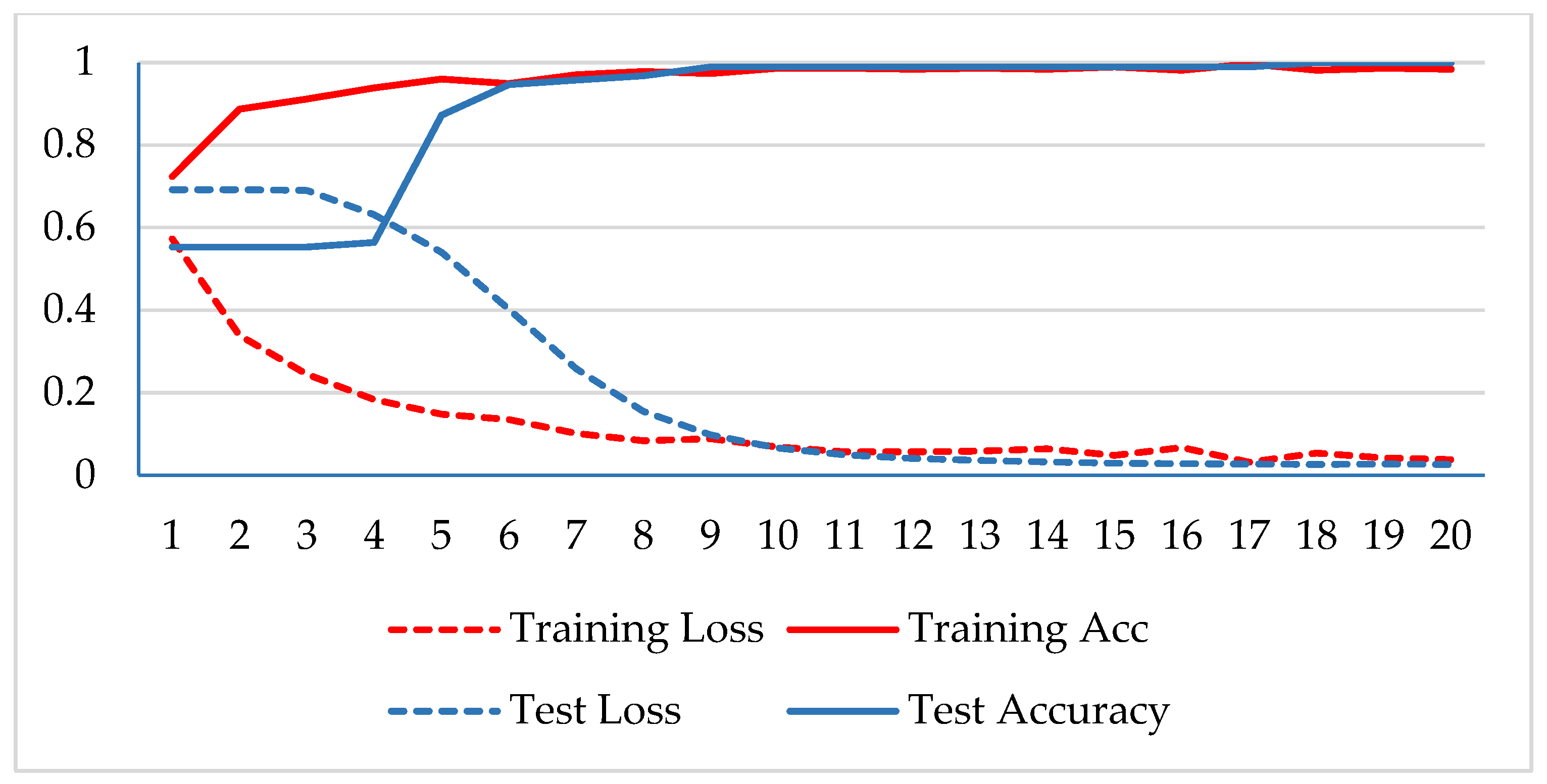
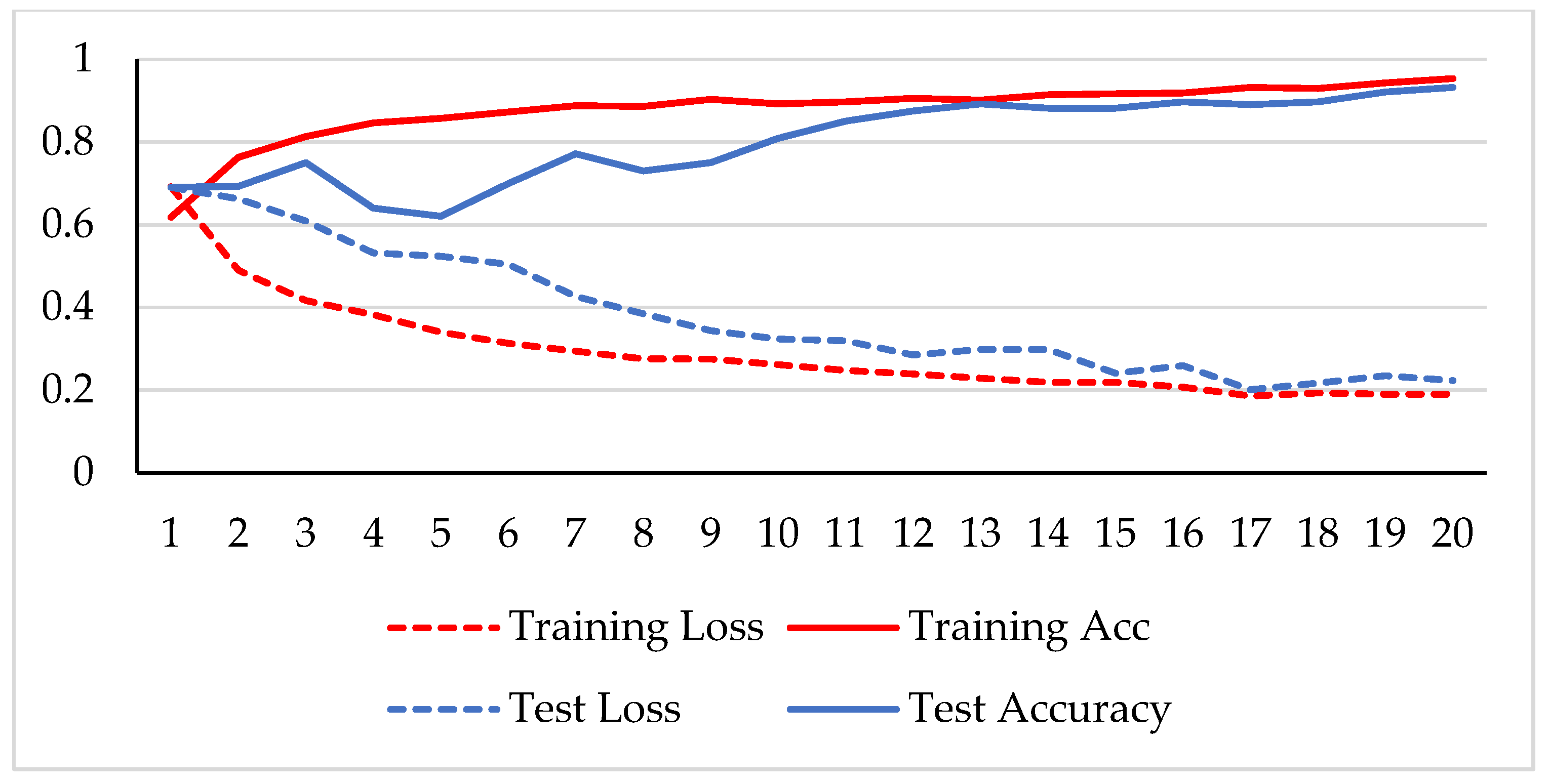
In the first phase, the network is verified for binary classification, i.e., benign and malignant type images, where malignant images include all four classes. A hold-out technique is used in simulation. The dataset is divided into two nonoverlapping subsets: a training and a test set. The training set is used to train the CNN model, while the test set is used to evaluate the model’s performance. The experiment is repeated for each magnification factor individually, and the model is analyzed using its training-testing accuracy and loss. Figure 5, Figure 6, Figure 7 and Figure 8 plot the accuracy and loss over epochs for both the training and testing datasets.
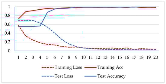
Figure 5.
Accuracy and loss analysis of the proposed network at a 40X magnification factor for binary classification.
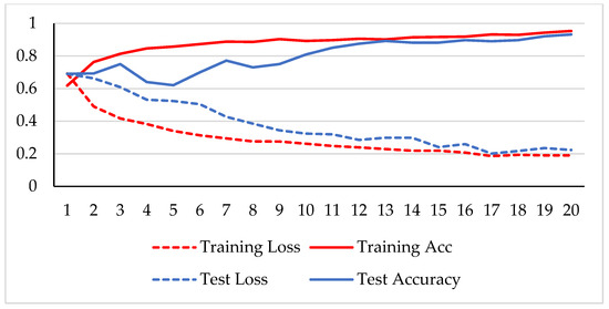
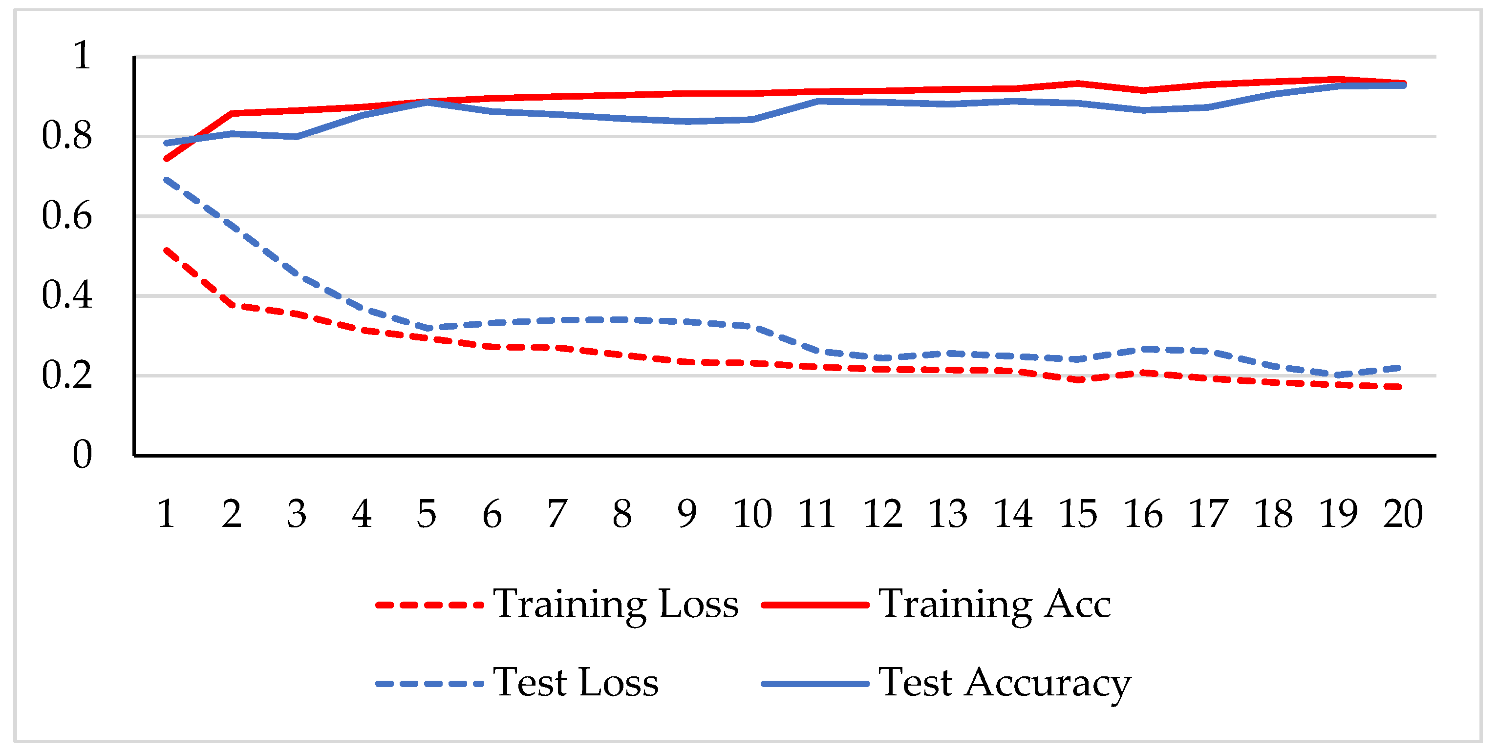
Figure 6.
Accuracy and loss analysis of the proposed network at a 100X magnification factor for binary classification.
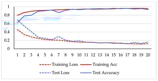
Figure 7.
Accuracy and loss analysis of the proposed network at a 200X magnification factor for binary classification.
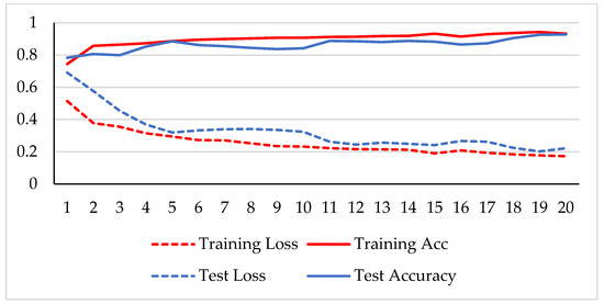
Figure 8.
Accuracy and loss analysis of the proposed network at a magnification factor of 400X for binary classification.
A stable training and testing accuracy was achieved after 12 epochs, and more than 90% accuracy was achieved after approximately 12 epochs. For 40X magnified images, the model’s accuracy is maximized, i.e., 99%, and for the remaining magnification factor, it achieved 96% accuracy. Thus, the extension of DenseNet using learnable residual network results in faster learning and better classification. The binary classification results are again evaluated using a confusion matrix to determine the detailed performance of the model. The results represent the performance of the classifier on test datasets whose true labels are known. Table 2 shows the performance evaluation using precision, recall, accuracy and F1 score, where TP represents the number of correct identifications of positive instances (i.e., the number of correct classifications of benign types), FP represents the number of negative instances classified as positive types (i.e., benign types misidentified as malignant types), FN represents the number of positive instances classified as negative types (i.e., malignant types misidentified as benign types), and TN represents the number of correct identifications of negative instances (i.e., correct classifications of malignant types). Using these four parameters, the model’s precision, recall, accuracy, and F1 score are calculated as follows.
Precision = TP/(TP + FP),
Recall = TP/(TP + FN),
Accuracy = (TP + TN)/(TP + FP + TN + FN)
F1-Score = 2 TP/(2xTP + FP + FN)
Table 2.
Proposed model’s performance analysis using test dataset for binary classification.
Table 2 shows that the model succeeded with an average accuracy of 96% among all the magnified factored images. The model received 100% test accuracy on images magnified at 40X and 94.65% accuracy for 400X magnification factor. The algorithm uses patches from high-resolution images, which could hinder its capability to extract features well. In cancer classification, malignant images are not misclassified, and high recalls are needed. The experiment showed that the average recall attained a significantly large value, i.e., 98.32%. The second phase of the experiment involved verifying the class of malignant images. The BreakHis dataset includes four types of malignant images, namely ductal carcinoma (DC), lobular carcinoma (LC), mucinous carcinoma (MC), and papillary carcinoma (PC) images. The same model is adopted for multiclass classification, changing its classification layer. Table 3 shows the training and testing images of the malignant lesions used to train and test the model.
Table 3.
Training and test datasets of malignant images for each magnification factor.
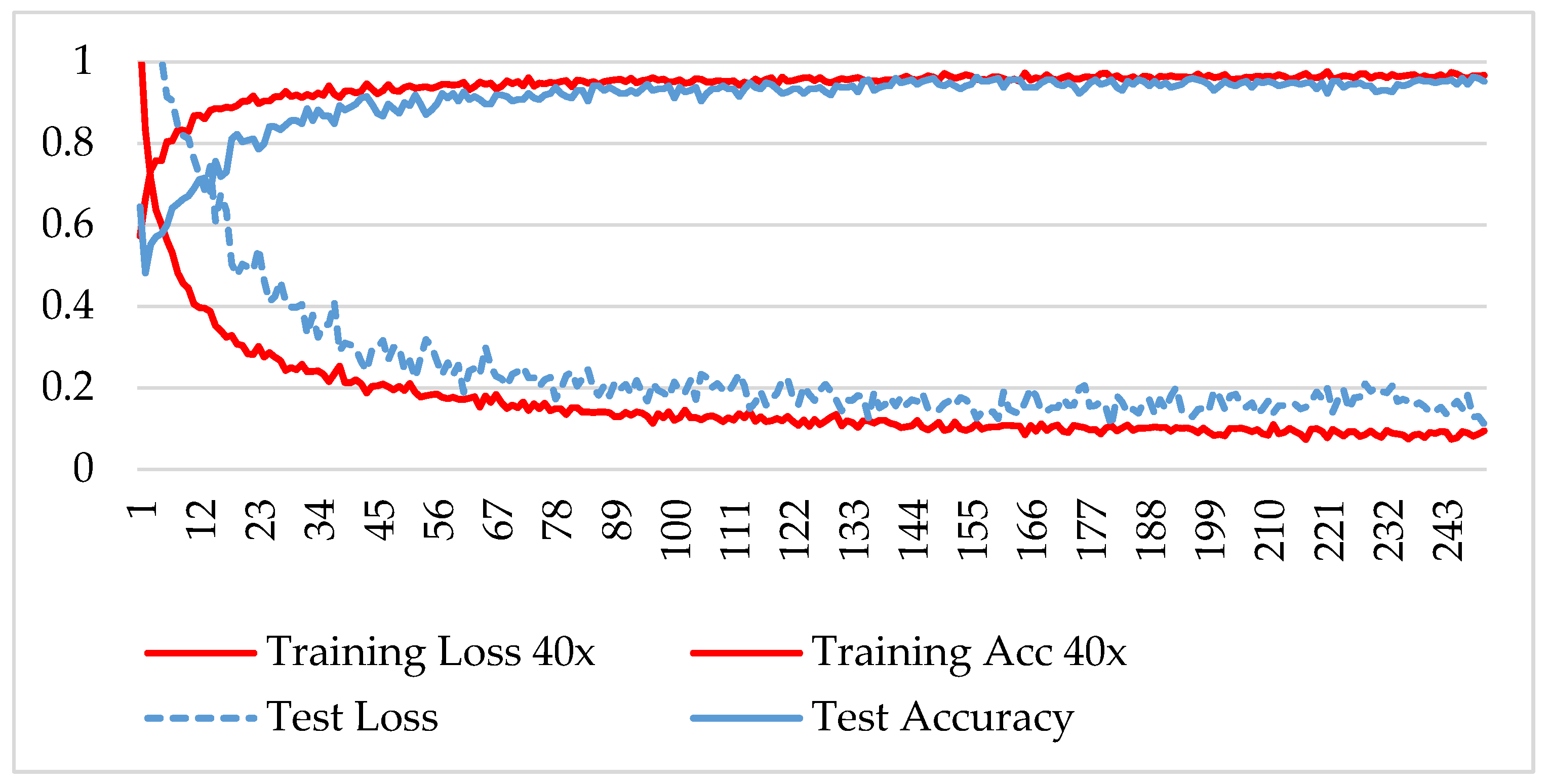
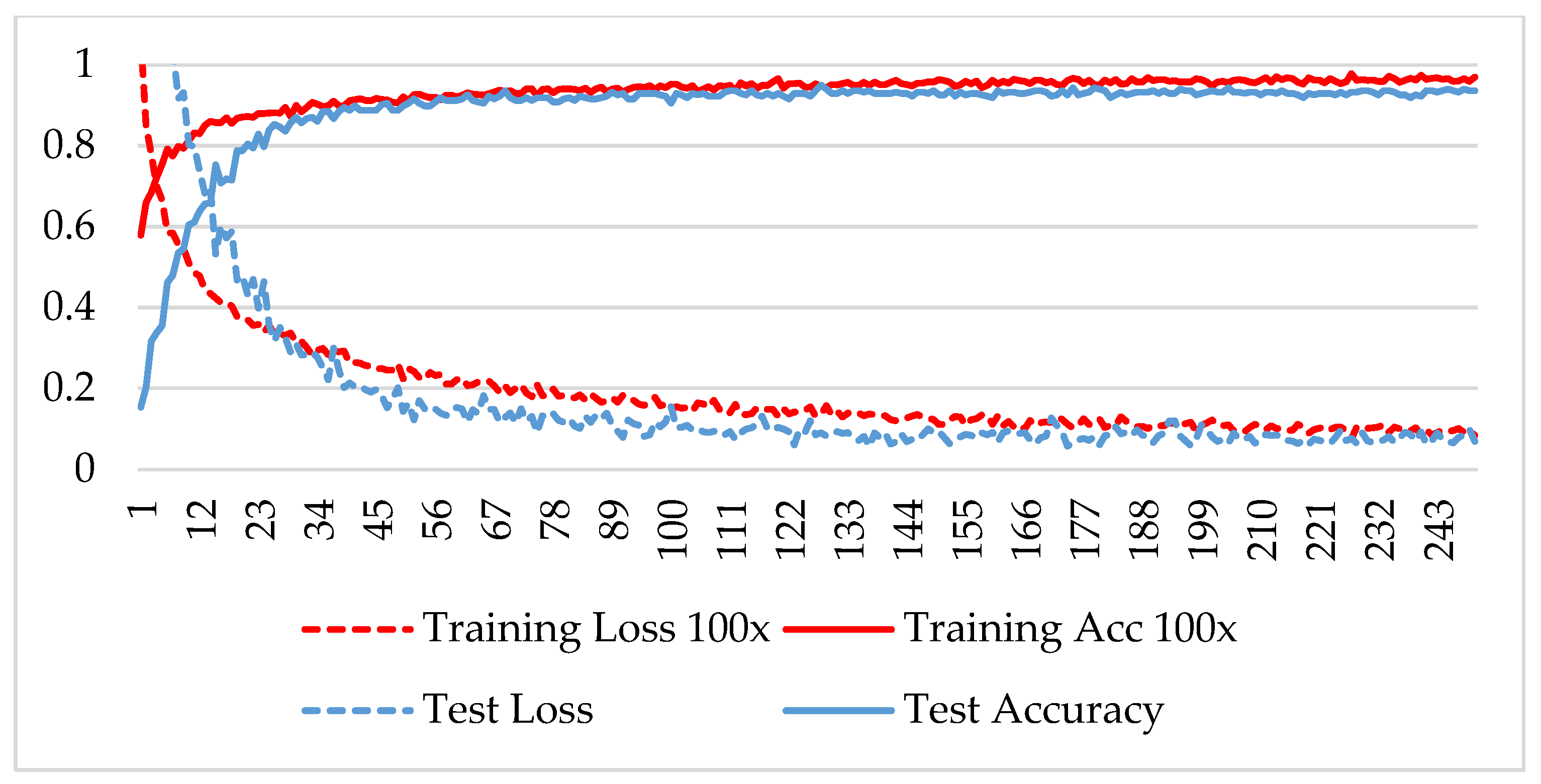
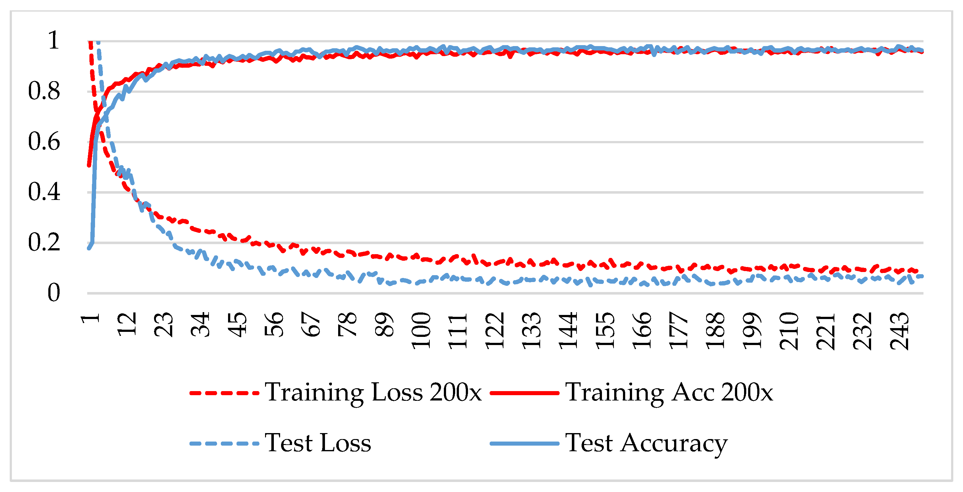
The model was trained over 250 epochs, and its accuracy and loss were analyzed for both the training and testing datasets. Figure 9, Figure 10, Figure 11 and Figure 12 show the accuracy and loss variation over time for each magnification factor. It is evident that training and test accuracies are increasing over epochs, and a small deviation between them shows that the model is not overfitted. The model received more than 95% accuracy at 73 epochs. At 400X magnification factor, the loss continuously decreases and eventually reaches 0.2% for the test dataset, and further training might not significantly improve its performance. The loss curve exhibits little fluctuations. This could be due to noisy images.
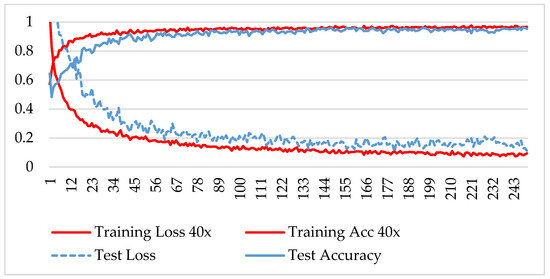
Figure 9.
Accuracy and loss analysis of the proposed network at a 40X magnification factor for malignant image classification.
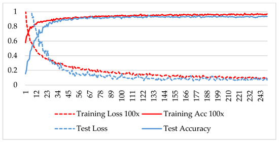
Figure 10.
Accuracy and loss analysis of the proposed network at a 100X magnification factor for malignant image classification.
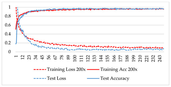
Figure 11.
Accuracy and loss analysis of the proposed network at a magnification factor of 200X for malignant image classification.
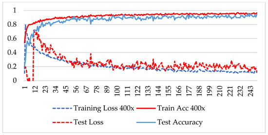
Figure 12.
Accuracy and loss analysis of the proposed network at a magnification factor of 400X for malignant image classification.
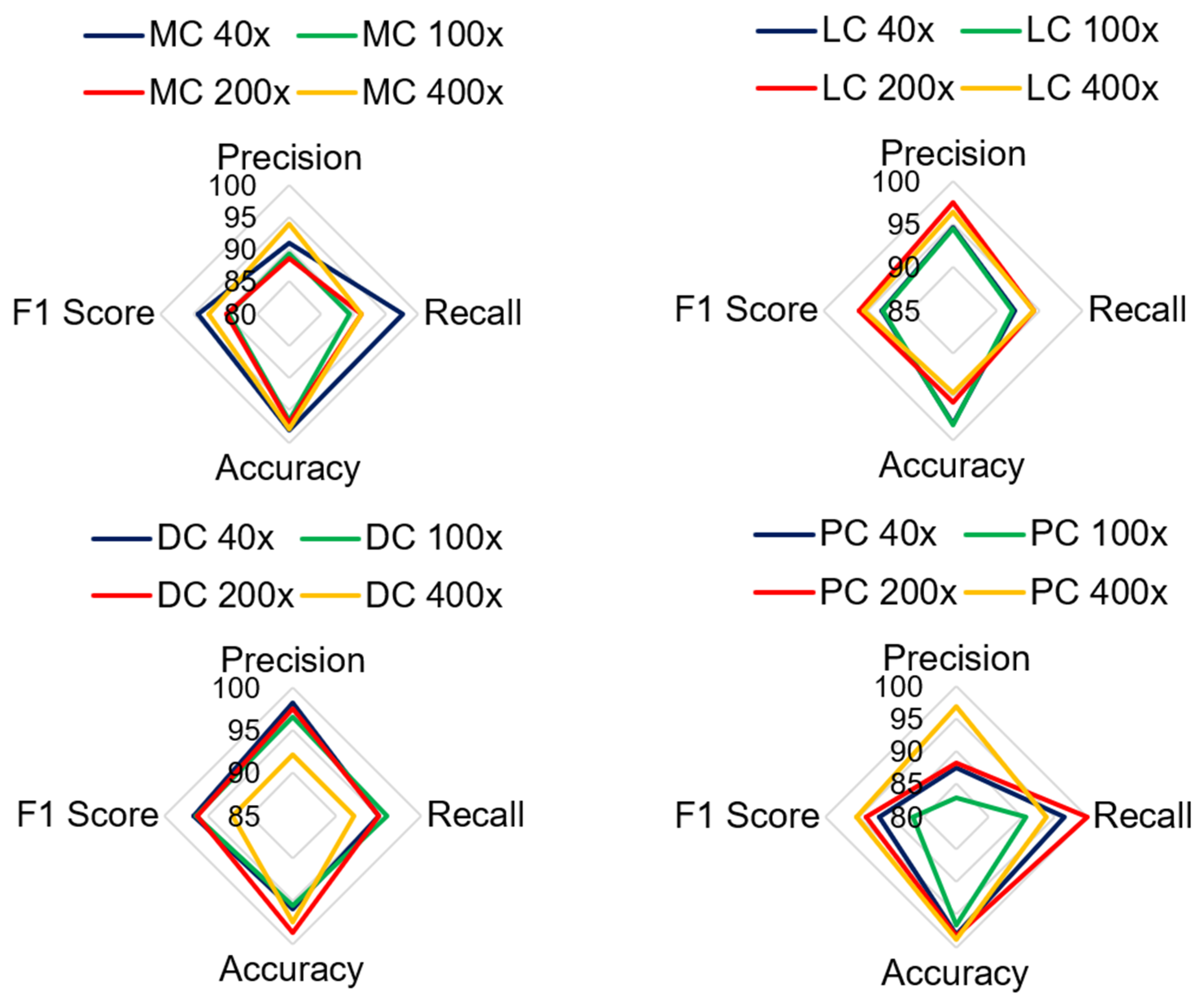
Table 4 shows the performance of the model in classifying malignant images. The average test accuracy for all magnification factors is 97.21%. The experiment shows that the proposed model identified DC, LC, and MC types of cancerous images well for all magnification factors. The F1-score for MC-type images slightly deviates at 100X and 200X magnification factors. The precision score for the PC class is less than that of the four classes. The lowest precision score is 82.86% for PC images at 100X magnification. There is no harmony between the precision and recall rate for PC classes, and therefore, its F1 score is lower than that of other types of classes. The classification accuracy for PC images is greater than 95%, which indicates that the model correctly predicts true classes. The lowest accuracy and F1 scores obtained by the model were 95.55% and 86.57%, respectively. Overall, the model is trained well for most sets of images; therefore, it can classify the negative class more accurately.
Table 4.
Performance analysis of the proposed model for multiclass classification of malignant images.
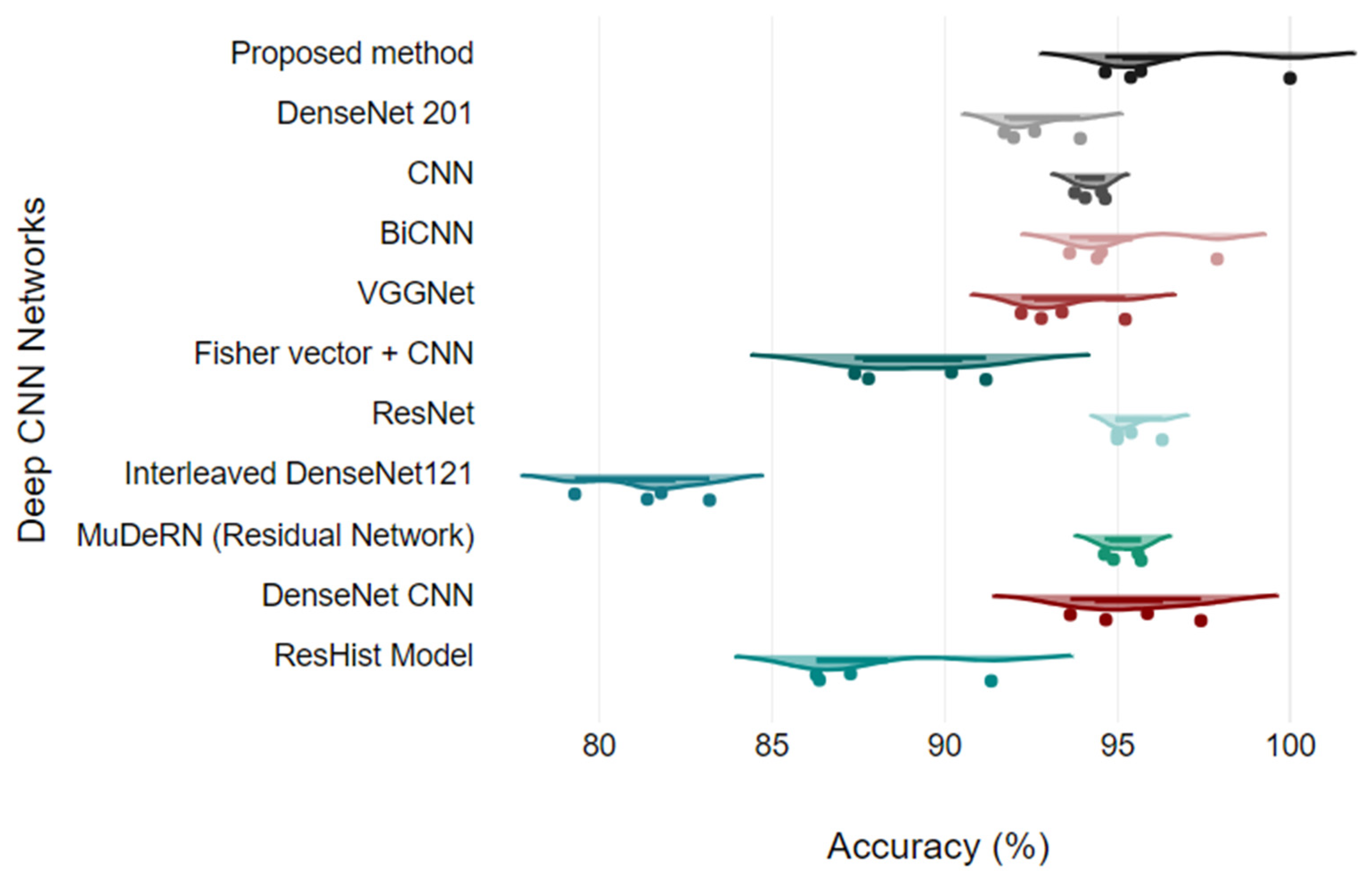
Figure 13 shows the analysis of all the quantitative parameters for each class. Figure 13 shows that the precision and F1 scores for the PC images are lower than those for the other classes, and the model predicts six PC images as either DC or MC type. Overall, the model achieved good performance for all the classes, with a 2.78% error rate. To validate the model, the proposed model is compared with the results of other studies that presented classification on the BreakHis dataset. The proposed model relies on DenseNet and a learnable residual layer; therefore, Table 5 shows a comparison of the proposed model with DenseNet or residual network-based networks for detecting malignant images, and Figure 14 shows a visual comparison.
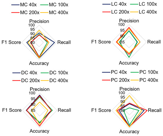
Figure 13.
Comparison of quantitative parameters for each malignant class.
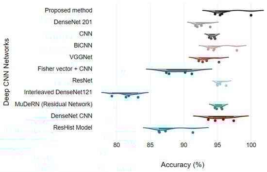
Figure 14.
Model comparison using Raincloud plots.
In [26], a VGG-16 network with a traditional classifier, SVM and RF, was proposed for cancer classification, and the model was validated for binary classes. Three different SVM kernel functions were tested for each magnification factor, and SVM using a polynomial kernel obtained the highest accuracy of 95.23% at the 200X magnification level. They observed that stain normalization of images in the network eventually reduces the accuracy of the model. In [27], a ResHist network, which uses a 152-layered convolutional neural network, was proposed to classify breast cancer histopathological images as binary only, achieving good accuracy and superiority over pretrained networks. The authors showed that ResNet outperformed the AlexNet, VGG16, and GoogLeNet deep-learning networks. The authors also evaluated ResNet features using different machine-learning classifiers, including K-nearest neighbors, support vector machines, and random forests. The authors achieved a maximum accuracy of 92.46% at the 200X zoom level using an SVM classifier.
Table 5.
Accuracy comparison of benign and malignant image classifications (binary classification).
Table 5.
Accuracy comparison of benign and malignant image classifications (binary classification).
| Method | 40X | 100X | 200X | 400X |
|---|---|---|---|---|
| ResHist Model [27] | 86.38 | 87.28 | 91.35 | 86.29 |
| DenseNet CNN [28] | 93.64 | 97.42 | 95.87 | 94.67 |
| MuDeRN (Residual Network) [29] | 95.60 | 94.89 | 95.69 | 94.63 |
| Interleaved DenseNet121 [30] | 81.8 | 79.3 | 81.4 | 83.2 |
| ResNet [31] | 96.3 | 95 | 95 | 95.4 |
| Fisher vector + CNN [32] | 90.2 | 91.2 | 87.8 | 87.4 |
| VGGNet [26] | 92.22 | 93.40 | 95.23 | 92.80 |
| BiCNN [33] | 97.89 | 93.62 | 94.54 | 94.42 |
| CNN [24] | 94.65 | 94.07 | 94.54 | 93.77 |
| DenseNet 201 [15] | 92.61 | 92 | 93.93 | 91.73 |
| Proposed method | 100 | 95.39 | 95.68 | 94.65 |
Nawaz et al. [34] used the DenseNet architecture for multiclass classification of malignant images and obtained a 95.4% classification rate. DenseNet uses a dense layer and transition layer instead of traditional convolutional, nonlinear, or pooling layers. In the dense block, outputs from previous layers are concatenated, allowing for the learning of features at different stages without the need for compression. This helps to avoid the explosion of parameters and reduces the complexity of the training process. Additionally, DenseNet can naturally scale to hundreds of layers without optimization difficulties, making it suitable for processing high-resolution images. By modifying the DenseNet model to handle histopathology images and using transfer learning, the proposed approach achieves high performance in breast cancer classification.
Li et al. [30] suggested the integration of DenseNet, a squeeze-and-excitation module, and a classification subnetwork for robust BC histological image classification. They tested the model on the BreakHis dataset, and the experiment was limited to binary classification. Experiments on the BreakHis dataset show improved performance compared to traditional CNN methods; however, their model’s maximum accuracy is 83.2% on the 400X dataset. In [32], the authors used Fisher vectors to obtain discriminative features from the texture region of histopathological images and embedded these features with a multilayer CNN network. Their model achieved 90.2% accuracy at all zoom levels. Eltoukhy et al. [31] used a residual learning approach to solve the problem of deep layers in the network and classified the BreakHis dataset into eight classes, namely, four benign types and four malignant types. This residual network succeeded with 96% average accuracy. Gandomkar et al. [29] designed a deep residual network to classify malignant images. They trained three different residual networks consisting of 50, 101, and 152 layers. Initially, images were classified as binary or malignant, and later, further subclassification of images was performed using a voting-based method.
In reference [33], the authors presented the BiCNN network using the GoogLeNet network, which provides a network-in-network architecture comparable to that of the AlexNet and VGG16 networks. The authors validated the model for the binary class with a maximum accuracy of 97%. Subclass classification is not presented. Bardou et al. [35] used handcrafted features, i.e., SURF and DSIFT, for classification and tested two models, i.e., SVM and CNN. Later, they configured CNNs and SVMs to improve the classification rate. Their CNN model was able to classify benign and malignant images at a rate of 94.65%; however, the model did not perform well for multiclass classification. Zerouaoui and Idri [15] tested various deep-learning models for feature extraction, including VGG, Inception V3, MobileNet V2, ResNet50, ResNet V2, and DenseNet 201, along with various classifiers, including MLP, SVM, DT, and KNN. They observed the best classification rate for DenseNet 201 with the MLP classifier. The multiclass classification was not presented by the author.
In reference [36], a semisupervised CNN model was proposed by the author. Initially, the model was trained for labeled data. Later, the trained model was tested for unlabeled data, and pseudolabels were generated from the prediction. These labeled images were used along with the training dataset to retrain the model. Thus, the model was trained twice, and it achieved 99.47% accuracy, with the top 5% to 10% of the images being pseudolabeled during retraining. However, the model did not perform well for multiclass classification. Joseph et al. [37] used handcrafted features with a deep CNN network. They obtained Hu-moment, colored histogram, and Haralick texture features from the images, and the CNN was trained using these features for multiclass classification. It was observed that their approach achieved accuracies of 90.87%, 89.57%, 91.58%, and 88.67% for each magnification factor.
Alkassar et al. [38] initially obtained shallow features and deep features using Dense and Xception architectures for binary and multiclass classification. Later, they used an ensemble of classifiers with the maximum rule to make a prediction. They observed that shallow features obtained using separable convolution in a dense network gave better classification than deep features for multiclass classification. The accuracies of these algorithms are listed in Table 6. A transfer learning approach on ResNet 18 was used in [39]. Initially, the images were normalized, and a trained ResNet 18 model was fine-tuned on images from the BreakHis dataset for multiclass classification. They evaluated and compared different ResNet architectures. ResNet18 achieved an average accuracy of 92.03%. The proposed model uses a learnable residual network after the convolutional layer of DenseNet. The DenseNet model provides spatial features, and the learnable residual network provides residual features from the convolutional features and pretrained features. The integration of both features helps to obtain distinct features for classification. Overall, the learning of the residual network helps to efCNNs valuate the booth course and find details from the histopathology images; therefore, the proposed model trained well and was able to classify better than other DenseNet and ResNet architectures. Table 6 shows that the model succeeded with average accuracies of 97.59%, 96.76%, 97.35%, and 97.20% for magnification factors of 40X, 100X, 200X and 400X, respectively.
Table 6.
Comparison of multiclass classification results at each magnification factor.
5. Conclusions
Among the many cancer disorders, breast cancer is at the top of the list. The prevalence of this illness is increasing daily, particularly among women. The death rate is relatively significant if this condition is not recognized in a timely manner. CNN models, which have powerful classification ability for images, can yield faster and better classifications than conventional methods. This paper aimed to improve breast cancer classification using histopathological images. A BreakHis dataset providing histopathological images at four magnification factors and multiclass categorization of both normal and malignant images were used in the experiment. The DenseNet architecture is modified by adding a residual learning network. A learnable residual network enhances the ability of the model to generate low-dimensional distinctive features. Thus, DenseNet’s convolution layers, followed by a learnable residual layer, maximize the chance of discriminating texture patterns. Later, the concatenation of both spatial features with residual features helps improve the overall classification rate. The experimental analysis of both the binary classification and malignant multiclass classification results revealed improvements in the classification results compared to those of other variants of the DenseNet architecture and various CNN models. One of the limitations of the network is that the precision score for PC images is lesser compared to other classes. Therefore, preprocessing these images can provide harmony between the precision and recall rate for PC images. The model is validated on a single dataset. The effectiveness of the model on diverse datasets would provide more robust evidence of its reliability. Future high-performance computer-aided diagnosis systems for other medical imaging tasks can be designed using the suggested method, which can be generalized. Another limitation of the proposed methodology is its inability to leverage multi-size training, as it relies on trained feature sets of pretrained networks. This dependency on pretrained models may limit applicability if the pretrained model is not trained well. This will be addressed in the future.
Funding
This research received no external funding.
Data Availability Statement
The data that support the findings of this study are openly available in reference number [25]. The authors confirm that the data supporting the findings of this study are available within the article [25].
Conflicts of Interest
The author declares no conflicts of interest.
References
- Hermansyah, D.; Firsty, N.N. The Role of Breast Imaging in Pre- and Post-Definitive Treatment of Breast Cancer. In Breast Cancer; Patel, K.C., Mayrovitz, H.N., Eds.; Exon Publications: Brisbane, Australia, 2022; pp. 83–99. [Google Scholar] [CrossRef]
- Gamble, P.; Jaroensri, R.; Wang, H.; Tan, F.; Moran, M.; Brown, T.; Flament-Auvigne, I.; Rakha, E.A.; Toss, M.; Dabbs, D.J.; et al. Determining breast cancer biomarker status and associated morphological features using deep learning. Commun. Med. 2021, 1, 14. [Google Scholar] [CrossRef] [PubMed]
- Liu, L.; Chen, J.; Fieguth, P.; Zhao, G.; Chellappa, R.; Pietikäinen, M. From BoW to CNN: Two Decades of Texture Representation for Texture Classification. Int. J. Comput. Vis. 2019, 127, 74–109. [Google Scholar] [CrossRef]
- Zhang, H.; Xue, J.; Dana, K. Deep TEN: Texture Encoding Network. In Proceedings of the 2017 IEEE Conference on Computer Vision and Pattern Recognition (CVPR), Honolulu, HI, USA, 21–26 July 2017; pp. 2896–2905. [Google Scholar] [CrossRef]
- Mao, S.; Rajan, D.; Chia, L.T. Deep residual pooling network for texture recognition. Pattern Recognit. 2021, 112, 107817. [Google Scholar] [CrossRef]
- Prusty, S.; Patnaik, S.; Dash, S.K. SKCV: Stratified K-fold cross-validation on ML classifiers for predicting cervical cancer. Front. Nanotechnol. 2022, 4, 972421. [Google Scholar] [CrossRef]
- Stegmuller, T.; Bozorgtabar, B.; Spahr, A.; Thiran, J.-P. ScoreNet: Learning Non-Uniform Attention and Augmentation for Transformer-Based Histopathological Image Classifica-tion. arXiv 2022, arXiv:2202.07570. [Google Scholar] [CrossRef]
- Gandomkar, Z.; Brennan, P.C.; Mello-Thoms, C. A framework for distinguishing benign from malignant breast histopathological images using deep residual networks. In Proceedings of the 14th International Workshop on Breast Imaging (IWBI 2018), Atlanta, GA, USA, 8–11 July 2018; Krupinski, E.A., Ed.; SPIE: Atlanta, GA, USA, 2018; p. 54. [Google Scholar] [CrossRef]
- Wakili, M.A.; Shehu, H.A.; Sharif, H.; Sharif, H.U.; Umar, A.; Kusetogullari, H.; Ince, I.F.; Uyaver, S. Classification of Breast Cancer Histopathological Images Using DenseNet and Transfer Learning. Comput. Intell. Neurosci. 2022, 2022, 8904768. [Google Scholar] [CrossRef] [PubMed]
- Vulli, A.; Srinivasu, P.N.; Sashank, M.S.K.; Shafi, J.; Choi, J.; Ijaz, M.F. Fine-Tuned DenseNet-169 for Breast Cancer Metastasis Prediction Using FastAI and 1-Cycle Policy. Sensors 2022, 22, 2988. [Google Scholar] [CrossRef] [PubMed]
- Mewada, H.K.; Patel, A.V.; Hassaballah, M.; Alkinani, M.H.; Mahant, K. Spectral–Spatial Features Integrated Convolution Neural Network for Breast Cancer Classification. Sensors 2020, 20, 4747. [Google Scholar] [CrossRef] [PubMed]
- Liu, Y.; Liu, X.; Qi, Y. Adaptive Threshold Learning in Frequency Domain for Classification of Breast Cancer Histopathological Images. Int. J. Intell. Syst. 2024, 2024, 9199410. [Google Scholar] [CrossRef]
- Salunkhe, P.B.; Patil, P.S. Rapid tri-net: Breast cancer classification from histology images using rapid tri-attention network. Multimedia Tools Appl. 2024, 83, 1–31. [Google Scholar] [CrossRef]
- Patel, H.; Mewada, H. Dictionary Properties for Sparse Representation: Implementation and Analysis. J. Artif. Intell. 2017, 11, 1–8. [Google Scholar] [CrossRef]
- Zerouaoui, H.; Idri, A. Deep hybrid architectures for binary classification of medical breast cancer images. Biomed. Signal Process. Control 2021, 71, 103226. [Google Scholar] [CrossRef]
- Wang, P.; Wang, J.; Li, Y.; Li, P.; Li, L.; Jiang, M. Automatic classification of breast cancer histopathological images based on deep feature fusion and enhanced routing. Biomed. Signal Process. Control 2020, 65, 102341. [Google Scholar] [CrossRef]
- Pandey, A.; Kumar, A. An integrated approach for breast cancer classification. Multimed. Tools Appl. 2023, 82, 33357–33377. [Google Scholar] [CrossRef]
- Chollet, F. Xception: Deep learning with depthwise separable convolutions. In Proceedings of the 2017 IEEE Conference on Computer Vision and Pattern Recognition (CVPR), Honolulu, HI, USA, 21–26 July 2017; pp. 1800–1807. [Google Scholar] [CrossRef]
- Naderan, M.; Zaychenko, Y. Convolutional Autoencoder Application for Breast Cancer Classification. In Proceedings of the 2020 IEEE 2nd International Conference on System Analysis & Intelligent Computing (SAIC), Kyiv, Ukraine, 5–9 October 2020; pp. 1–4. [Google Scholar] [CrossRef]
- Jiang, Y.; Chen, L.; Zhang, H.; Xiao, X. Breast cancer histopathological image classification using convolutional neural networks with small SE-ResNet module. PLoS ONE 2019, 14, e0214587. [Google Scholar] [CrossRef] [PubMed]
- Liu, K.; Liu, Z.; Liu, S. Semi-supervised breast histopathological image classification with self-training based on non-linear distance metric. IET Image Process. 2022, 16, 3164–3176. [Google Scholar] [CrossRef]
- Kolla, B.; P, V. An integrated approach for magnification independent breast cancer classification. Biomed. Signal Process. Control 2024, 88, 105594. [Google Scholar] [CrossRef]
- Zhou, Y.; Zhang, C.; Gao, S. Breast Cancer Classification from Histopathological Images Using Resolution Adaptive Network. IEEE Access 2022, 10, 35977–35991. [Google Scholar] [CrossRef]
- Xu, Y.; Li, F.; Chen, Z.; Liang, J.; Quan, Y. Encoding spatial distribution of convolutional features for texture representation. Adv. Neural Inf. Process. Syst. 2021, 34, 22732–22744. [Google Scholar]
- Spanhol, F.A.; Oliveira, L.S.; Petitjean, C.; Heutte, L. A Dataset for Breast Cancer Histopathological Image Classification. IEEE Trans. Biomed. Eng. 2015, 63, 1455–1462. [Google Scholar] [CrossRef] [PubMed]
- Kumar, A.; Singh, S.K.; Saxena, S.; Lakshmanan, K.; Sangaiah, A.K.; Chauhan, H.; Shrivastava, S.; Singh, R.K. Deep feature learning for histopathological image classification of canine mammary tumors and human breast cancer. Inf. Sci. 2019, 508, 405–421. [Google Scholar] [CrossRef]
- Gour, M.; Jain, S.; Kumar, T.S. Residual learning based CNN for breast cancer histopathological image classification. Int. J. Imaging Syst. Technol. 2020, 30, 621–635. [Google Scholar] [CrossRef]
- Nguyen, P.T.; Nguyen, T.T.; Nguyen, N.C.; Le, T.T. Multiclass Breast Cancer Classification Using Convolutional Neural Network. In Proceedings of the 2019 International Symposium on Electrical and Electronics Engineering (ISEE), Ho Chi Minh, Vietnam, 10–12 October 2019; pp. 130–134. [Google Scholar] [CrossRef]
- Gandomkar, Z.; Brennan, P.C.; Mello-Thoms, C. MuDeRN: Multi-category classification of breast histopathological image using deep residual networks. Artif. Intell. Med. 2018, 88, 14–24. [Google Scholar] [CrossRef]
- Li, X.; Shen, X.; Zhou, Y.; Wang, X.; Li, T.-Q. Classification of breast cancer histopathological images using interleaved DenseNet with SENet (IDSNet). PLoS ONE 2020, 15, e0232127. [Google Scholar] [CrossRef] [PubMed]
- Eltoukhy, M.M.; Hosny, K.M.; Kassem, M.A. Classification of Multiclass Histopathological Breast Images Using Residual Deep Learning. Comput. Intell. Neurosci. 2022, 2022, 9086060. [Google Scholar] [CrossRef]
- Song, Y.; Chang, H.; Huang, H.; Cai, W. Supervised Intra-embedding of Fisher Vectors for Histopathology Image Classification. In Proceedings of the International Conference on Medical Image Computing and Computer-Assisted Intervention, Quebec City, QC, Canada, 11–13 September 2017; Descoteaux, M., Maier-Hein, L., Franz, A., Jannin, P., Collins, D.L., Duchesne, S., Eds.; Lecture Notes in Computer Science, Volume 10435. Springer International Publishing: Cham, Switzerland, 2017; pp. 99–106. [Google Scholar] [CrossRef]
- Wei, B.; Han, Z.; He, X.; Yin, Y. Deep learning model based breast cancer histopathological image classificationin. In Proceedings of the 2017 IEEE 2nd International Conference on Cloud Computing and Big Data Analysis (ICCCBDA), Chengdu, China, 28–30 April 2017; pp. 348–353. [Google Scholar]
- Nawaz, M.; Sewissy, A.A.; Hassan, T. Multi-Class Breast Cancer Classification using Deep Learning Convolutional Neural Network. Int. J. Adv. Comput. Sci. Appl. 2018, 9, 316–322. [Google Scholar] [CrossRef]
- Bardou, D.; Zhang, K.; Ahmad, S.M. Classification of Breast Cancer Based on Histology Images Using Convolutional Neural Networks. IEEE Access 2018, 6, 24680–24693. [Google Scholar] [CrossRef]
- Asare, S.K.; You, F.; Nartey, O.T. A Semisupervised Learning Scheme with Self-Paced Learning for Classifying Breast Cancer Histopathological Images. Comput. Intell. Neurosci. 2020, 2020, 8826568. [Google Scholar] [CrossRef] [PubMed]
- Joseph, A.A.; Abdullahi, M.; Junaidu, S.B.; Ibrahim, H.H.; Chiroma, H. Improved multi-classification of breast cancer histopathological images using handcrafted features and deep neural network (dense layer). Intell. Syst. Appl. 2022, 14, 200066. [Google Scholar] [CrossRef]
- Alkassar, S.; Jebur, B.A.; Abdullah, M.A.M.; Al-Khalidy, J.H.; Chambers, J.A. Going deeper: Magnification-invariant approach for breast cancer classification using histopathological images. IET Comput. Vis. 2021, 15, 151–164. [Google Scholar] [CrossRef]
- Boumaraf, S.; Liu, X.; Zheng, Z.; Ma, X.; Ferkous, C. A new transfer learning based approach to magnification dependent and independent classification of breast cancer in histopathological images. Biomed. Signal Process. Control 2020, 63, 102192. [Google Scholar] [CrossRef]


Disclaimer/Publisher’s Note: The statements, opinions and data contained in all publications are solely those of the individual author(s) and contributor(s) and not of MDPI and/or the editor(s). MDPI and/or the editor(s) disclaim responsibility for any injury to people or property resulting from any ideas, methods, instructions or products referred to in the content. |
© 2024 by the author. Licensee MDPI, Basel, Switzerland. This article is an open access article distributed under the terms and conditions of the Creative Commons Attribution (CC BY) license (https://creativecommons.org/licenses/by/4.0/).