
Numerical Study on Aerodynamic Noise Reduction in Passenger Car with Fender Shape Optimization


Abstract
1. Introduction
2. Simulation Methods
2.1. CFD Simulation Method
2.2. Aerodynamic Noise Analysis
3. Optimization Methods
3.1. Optimization of Fender Configuration Based on FFD Method
3.2. Parameterized Scheme for Fender Configuration
3.3. Design of Experiments
3.4. Construction Approximate Models
4. Results and Analysis
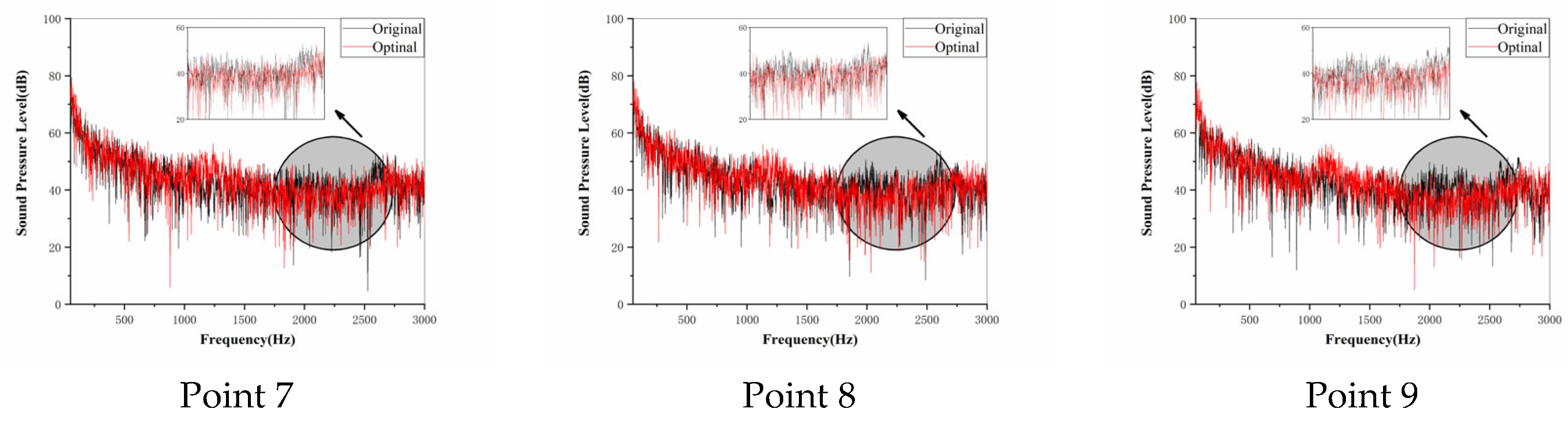
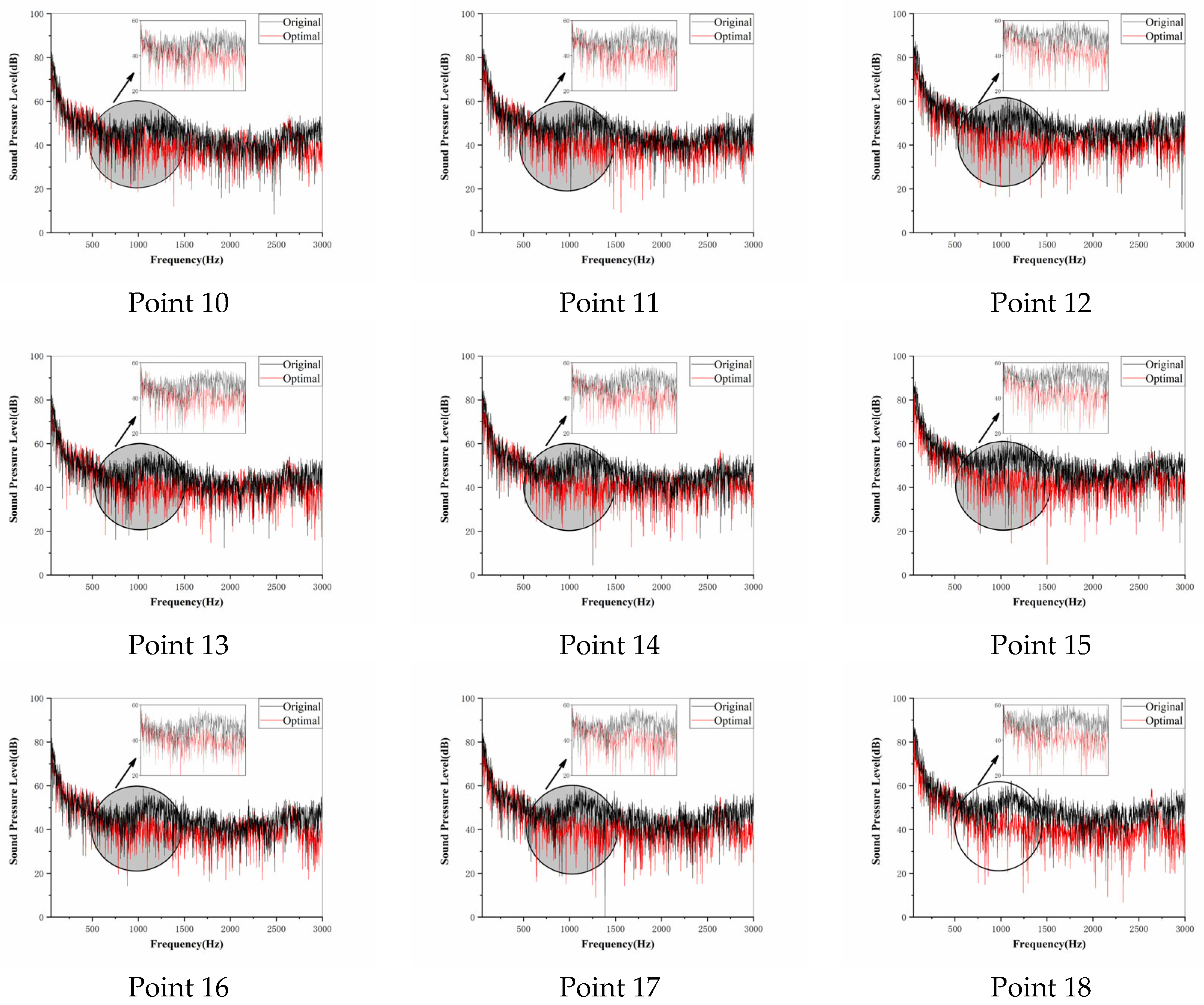
4.1. SPL Characteristics
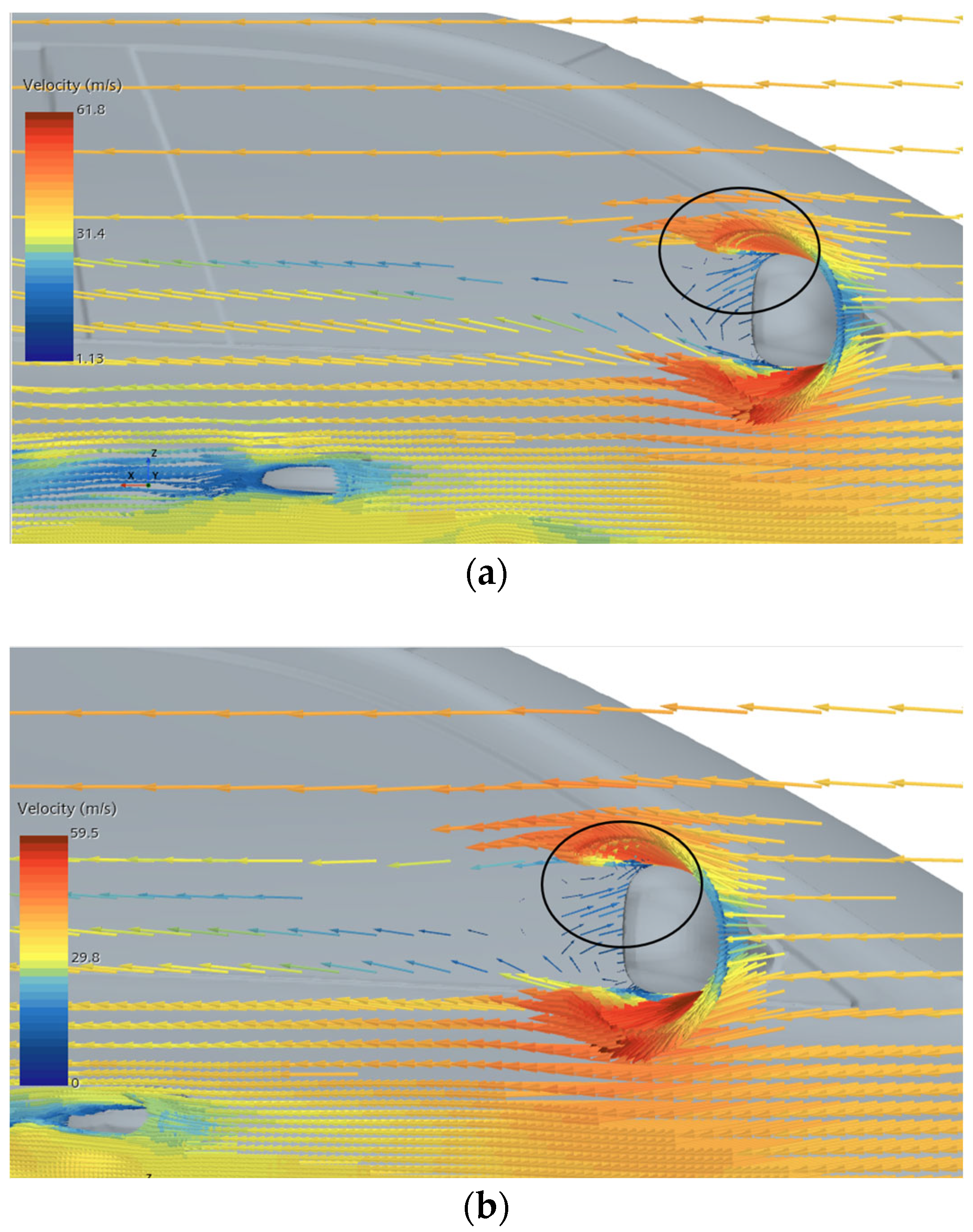
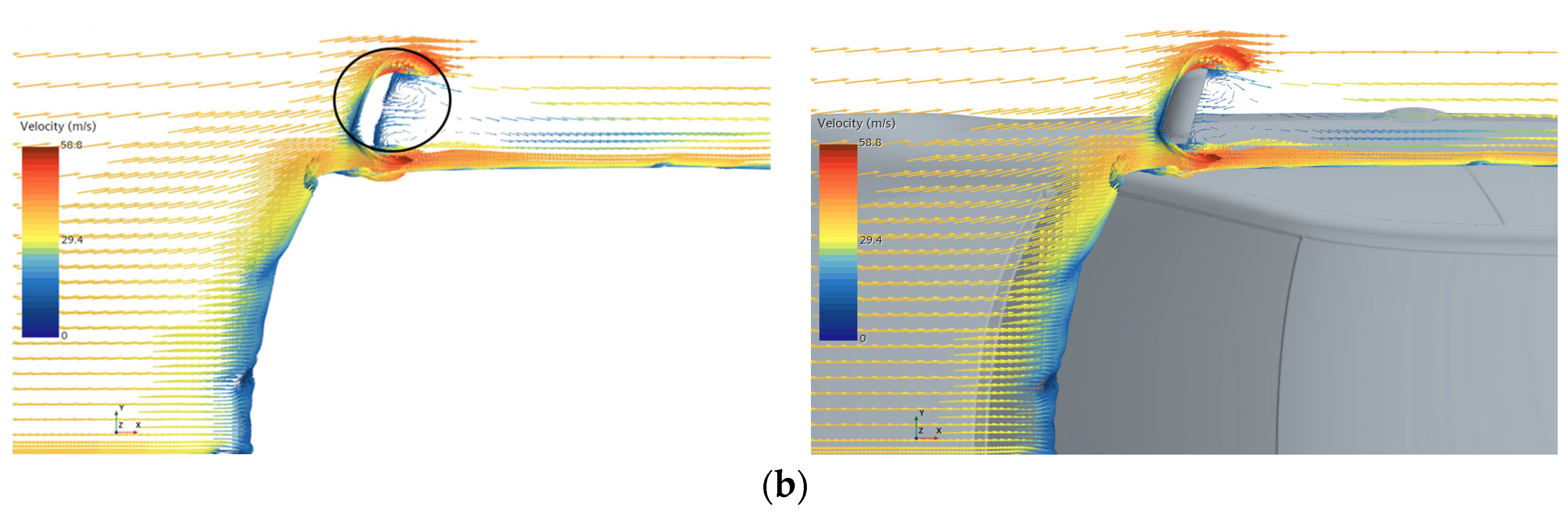
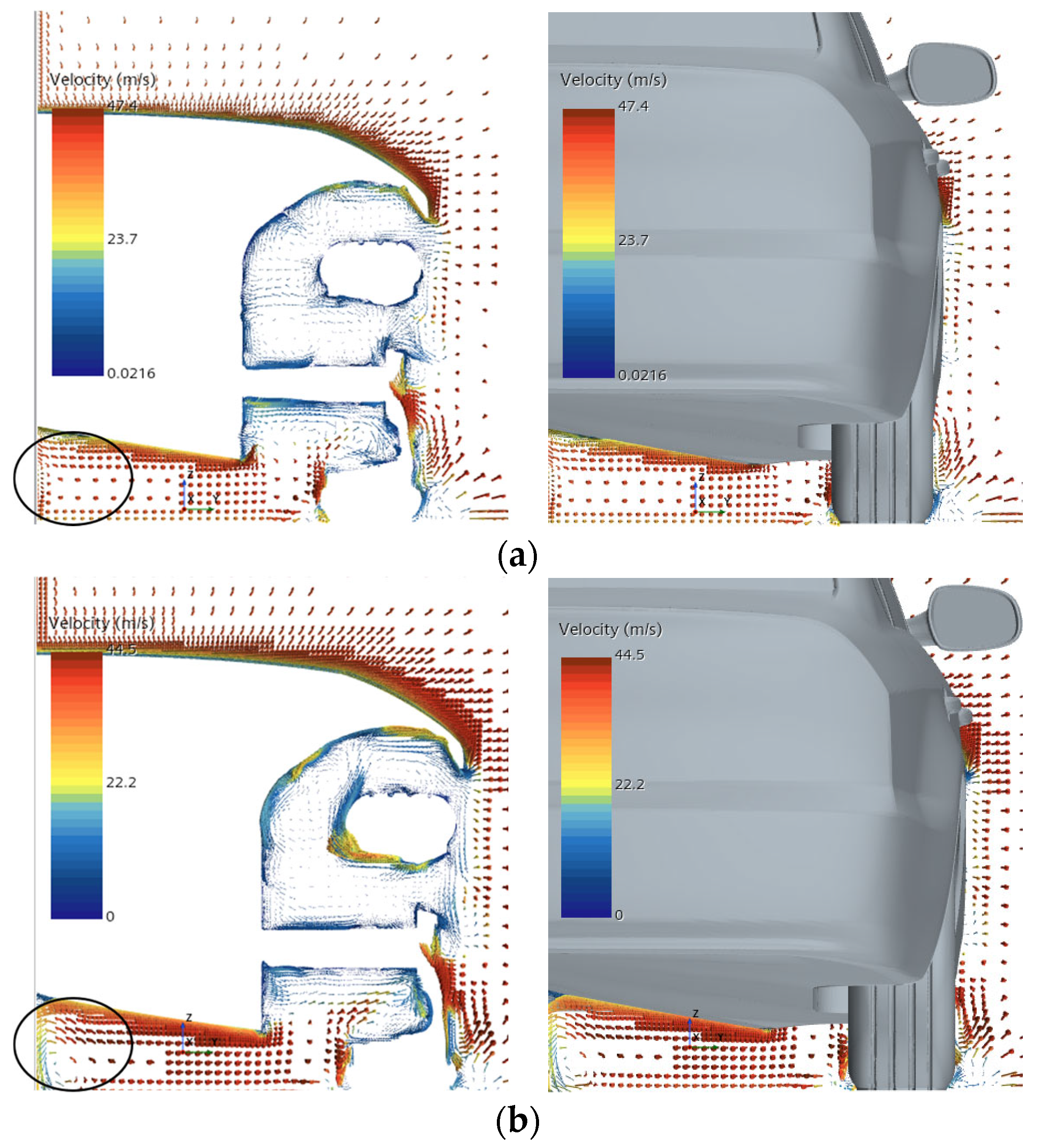
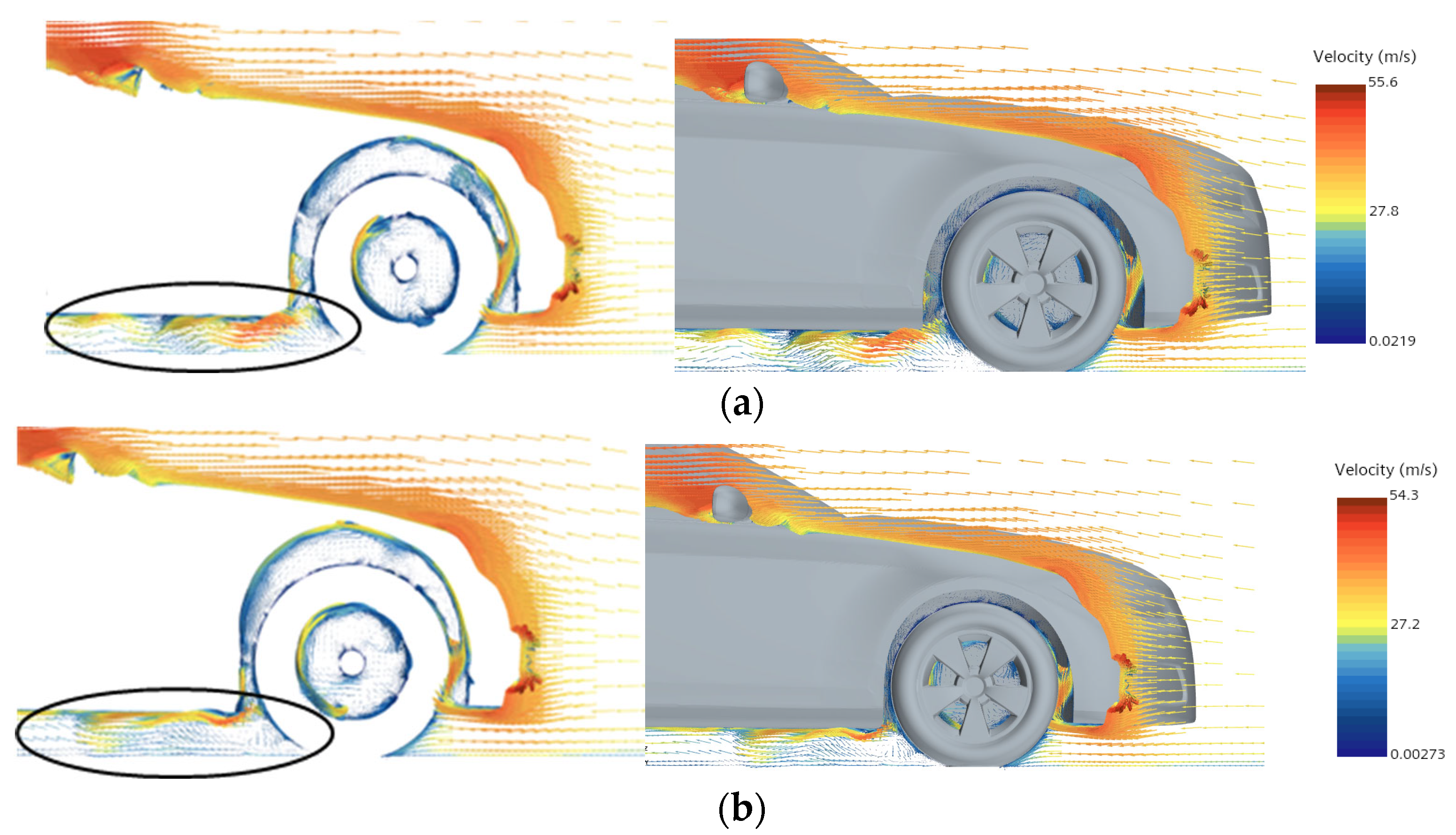
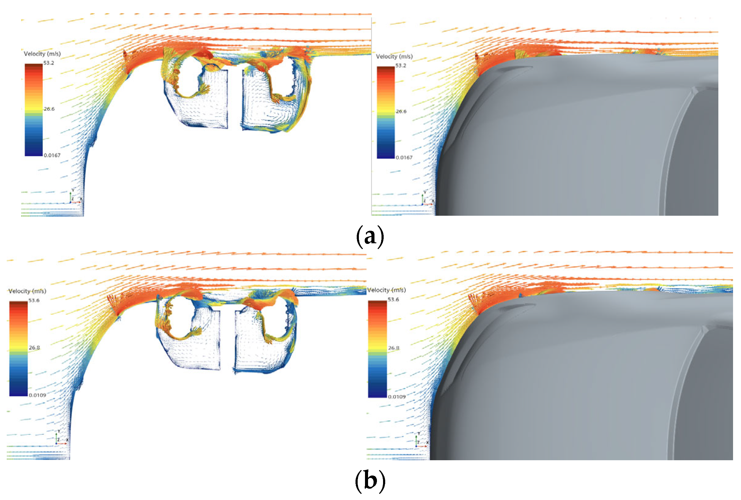
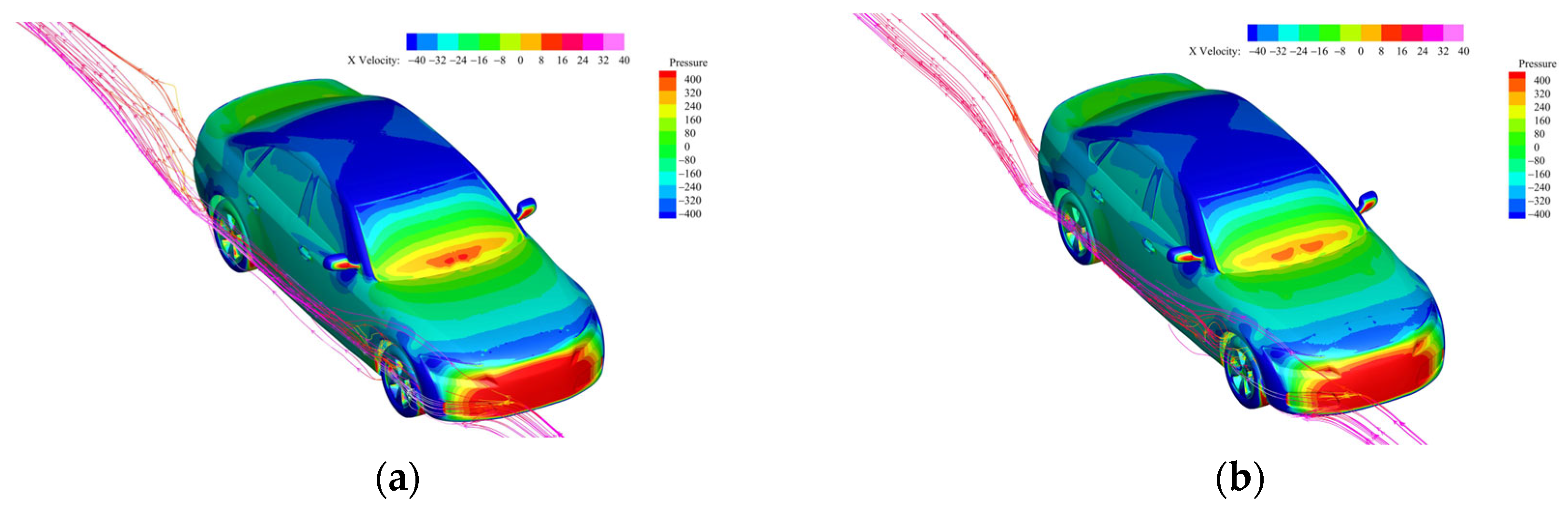
4.2. Velocity Vector Analysis
5. Conclusions
Author Contributions
Funding
Data Availability Statement
Conflicts of Interest
References
- Wolf, A.; Gaertner, U.; Droege, T. Noise Reduction and Sound Design for Diesel Engines—An Achievable Development Target for US Passenger Cars? SAE Technical Paper 2003-01-1719; SAE International: Warrendale, PA, USA, 2003. [Google Scholar] [CrossRef]
- Zhou, H.; Qin, R.; Wang, G.; Xin, L.; Wang, Q.; Zheng, Z. Comparative analysis of the aerodynamic behavior on Ahmed body mounted with different wheel configurations. Proc. Inst. Mech. Eng. Part D J. Automob. Eng. 2024, 238, 128–146. [Google Scholar] [CrossRef]
- Yoo, B.K.; Chang, K.-J. Road Noise Reduction Using a Source Decomposition and Noise Path Analysis; SAE Technical Paper 2005-01-2502; SAE International: Warrendale, PA, USA, 2005. [Google Scholar] [CrossRef]
- Chuang, J.S.; Lin, H.H.; Chen, Y.Y.; Su, T.K. Study of Tire Noise for Vehicle Noise Control; SAE Technical Paper 2005-01-2415; SAE International: Warrendale, PA, USA, 2005. [Google Scholar] [CrossRef]
- Dumas, L. CFD-Based Optimization for Automotive Aerodynamics. In Optimization and Computational Fluid Dynamics; Springer: Berlin/Heidelberg, Germany, 2008; pp. 191–215. [Google Scholar]
- Li, H. Analysis and optimization of aerodynamic noise in vehicle based on acoustic perturbation equations and statistical energy analysis. SAE Int. J. Veh. Dyn. Stab. 2022, 6, 223–232. [Google Scholar] [CrossRef]
- Lian, Y.; Luo, Q.; Zhang, F.; Zhang, R.; Zhang, Y. Automotive Aerodynamics Development Based on Shape Optimization Method. Automot. Eng. 2022, 44, 1619–1626. [Google Scholar]
- Watkins, S. Aerodynamic noise and its refinement in vehicles. In Vehicle Noise and Vibration Refinement; Elsevier: Amsterdam, The Netherlands, 2010; pp. 219–234. [Google Scholar]
- Li, Y.; Kasaki, N.; Tsunoda, H.; Nakamura, T.; Nouzawa, T. Evaluation of Wind Noise Sources Using Experimental and Computational Methods; SAE Technical Paper 2006-01-0343; SAE International: Warrendale, PA, USA, 2006. [Google Scholar] [CrossRef]
- Kameier, F.; Wagner, T.; Horvat, I.; Ullrich, F. Experimental and numerical investigation of air dam aeroacoustics. ATZ Worldw. 2009, 111, 54–59. [Google Scholar] [CrossRef]
- Yang, M.; Zhao, Q.; Sun, Z.; Zhang, Y.; Liu, P. Mechanism analysis on the flow induced low-frequency noise in NEV. In Proceedings of the Society of Automotive Engineers (SAE)-China Congress, Shanghai, China, 25–27 October 2023; Springer: Berlin/Heidelberg, Germany, 2023; pp. 386–401. [Google Scholar]
- Chen, Y.-G.; Wang, X.-H.; Zhou, Y.-M. Numerical investigation on aerodynamic noises of the lateral window in vehicles. J. Vibroeng. 2017, 19, 6502–6518. [Google Scholar] [CrossRef]
- Ringwall, E. Aeroacoustic Sound Sources around the Wheels of a Passenger Car—A Computational Fluid Dynamics Study Using Steady State Models to Evaluate Main Sources of Flow Noise. Master’s Thesis, Gothenburg Chalmers University of Technology, Gothenburg, Sweden, 2017. [Google Scholar]
- Wang, Y.G.; Huang, X.S.; Liu, Y.; Shen, Z.; He, Y.Z. Experimental evaluation on vehicle aerodynamic noise performance. Int. J. Veh. Perform. 2018, 4, 155–174. [Google Scholar] [CrossRef]
- Sederberg, T.W.; Parry, S.R. Free-form deformation of solid geometric models. In Proceedings of the 13th Annual Conference on Computer Graphics and Interactive Techniques, Dallas, TX, USA, 18–22 August 1986; pp. 151–160. [Google Scholar]
- Yiping, W.; Tao, W.; Shuai, L. Aerodynamic drag reduction of vehicle based on free form deformation. J. Mech. Eng. 2017, 53, 135–143. [Google Scholar]
- Granados Casadó, P. Aerodynamic Optimization of an Electric Car Surface. Bachelor’s Thesis, Universitat Politècnica de Catalunya, Barcelona, España, 2022. [Google Scholar]
- Wang, K.; Han, Z.H.; Zhang, K.S.; Song, W.P. An efficient geometric constraint handling method for surrogate-based aerodynamic shape optimization. Eng. Appl. Comput. Fluid Mech. 2023, 17, e2153173. [Google Scholar] [CrossRef]
- Roshanian, J.; Ebrahimi, M. Latin hypercube sampling applied to reliability-based multidisciplinary design optimization of a launch vehicle. Aerosp. Sci. Technol. 2013, 28, 297–304. [Google Scholar] [CrossRef]
- Przysowa, K.; Łaniewski-Wołłk, Ł.; Rokicki, J. Shape optimisation method based on the surrogate models in the parallel asynchronous environment. Appl. Soft Comput. 2018, 71, 1189–1203. [Google Scholar] [CrossRef]
- Zhou, H.; Jiang, Z.; Wang, G.; Zhang, S. Aerodynamic characteristics of isolated loaded tires with different tread patterns: Experiment and simulation. Chin. J. Mech. Eng. 2021, 34, 1–16. [Google Scholar] [CrossRef]
- Wäschle, A. The Influence of Rotating Wheels on Vehicle Aerodynamics-Numerical And Experimental Investigations; SAE Technical Paper 2007-01-0107; SAE International: Warrendale, PA, USA, 2007. [Google Scholar] [CrossRef]
- Rüttgers, M.; Park, J.; You, D. Large-eddy simulation of turbulent flow over the DrivAer fastback vehicle model. J. Wind. Eng. Ind. Aerodyn. 2019, 186, 123–138. [Google Scholar] [CrossRef]
- Hong, L.; Yaohui, L.; Qingyang, W.; Xiaochun, Y.; Xiaobo, S.; Yanhui, T. Research on the influences of side-wing diffuser on automotive aerodynamic characteristics. Automot. Eng. 2021, 43, 1653–1661. [Google Scholar]
- Dawi, A.H.; Akkermans, R.A. Direct noise computation of a generic vehicle model using a finite volume method. Comput. Fluids 2019, 191, 104243. [Google Scholar] [CrossRef]
- Li, H.; Hao, Z.Y.; Zheng, X.; Shi, J.G.; Wang, L.W. LES-FEM coupled analysis and experimental research on aerodynamic noise of the vehicle intake system. Appl. Acoust. 2017, 116, 107–116. [Google Scholar] [CrossRef]
- Viana, F.A. A tutorial on Latin hypercube design of experiments. Qual. Reliab. Eng. Int. 2016, 32, 1975–1985. [Google Scholar] [CrossRef]
- Moody, J.; Darken, C.J. Fast learning in networks of locally-tuned processing units. Neural Comput. 1989, 1, 281–294. [Google Scholar] [CrossRef]
- Shuanbao, Y.; Dilong, G.; Guowei, Y. Aerodynamic optimization of high-speed train based on RBF mesh deformation. Chin. J. Theor. Appl. Mech. Mater. 2013, 45, 982–986. [Google Scholar]


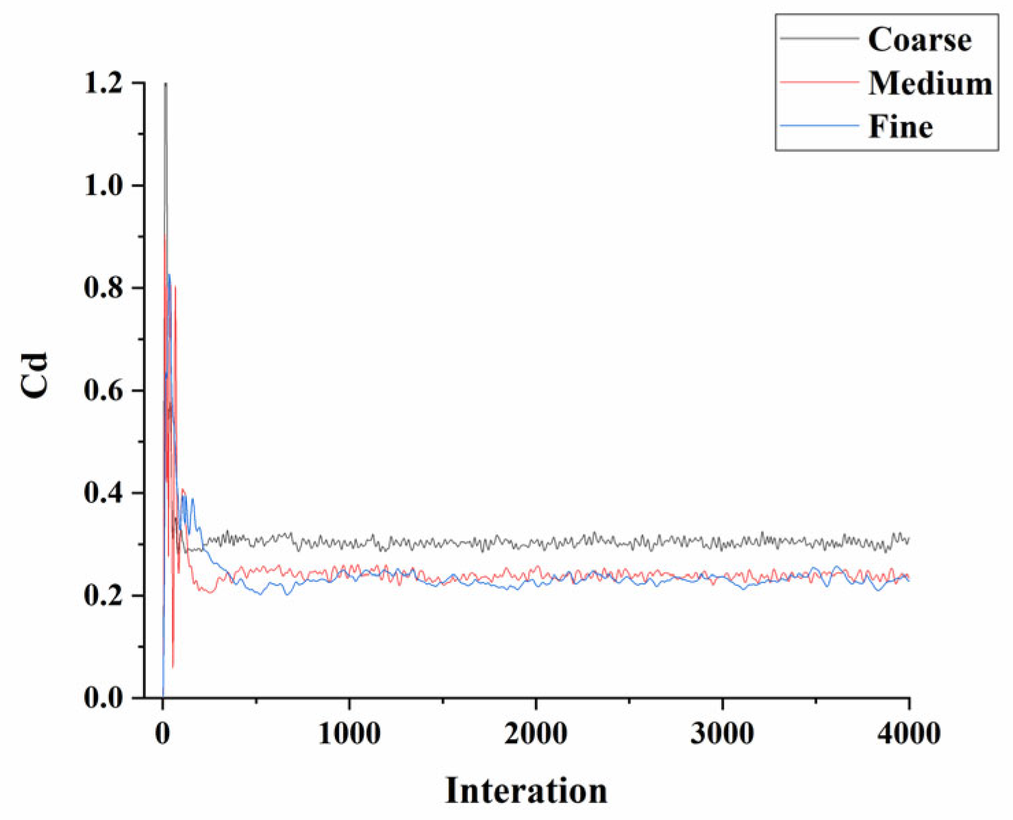
| Mesh | Body | Fender | Computational Domain | Cd |
|---|---|---|---|---|
| Coarse | 15~30 mm | 5~15 mm | 30~200 mm | 0.312 |
| Medium | 10~15 mm | 1~5 mm | 15~200 mm | 0.245 |
| Fine | 5~10 mm | 1~4 mm | 10~200 mm | 0.235 |
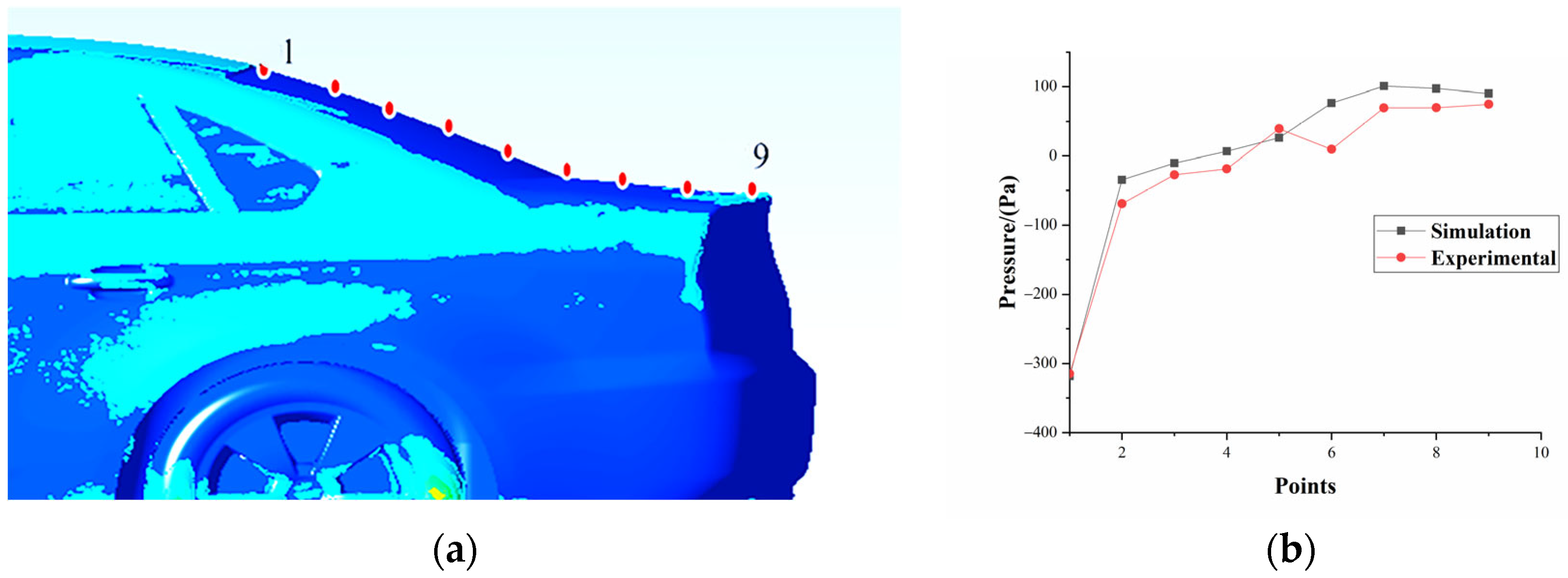
| Parameters | Projection Area/m2 | Cd |
|---|---|---|
| Wind tunnel experiments | 2.173 | 0.250 |
| Numerical simulation | 2.168 | 0.245 |
| Errors/% | 0.23 | 2.00 |
| Lower/m | Upper/m | |
|---|---|---|
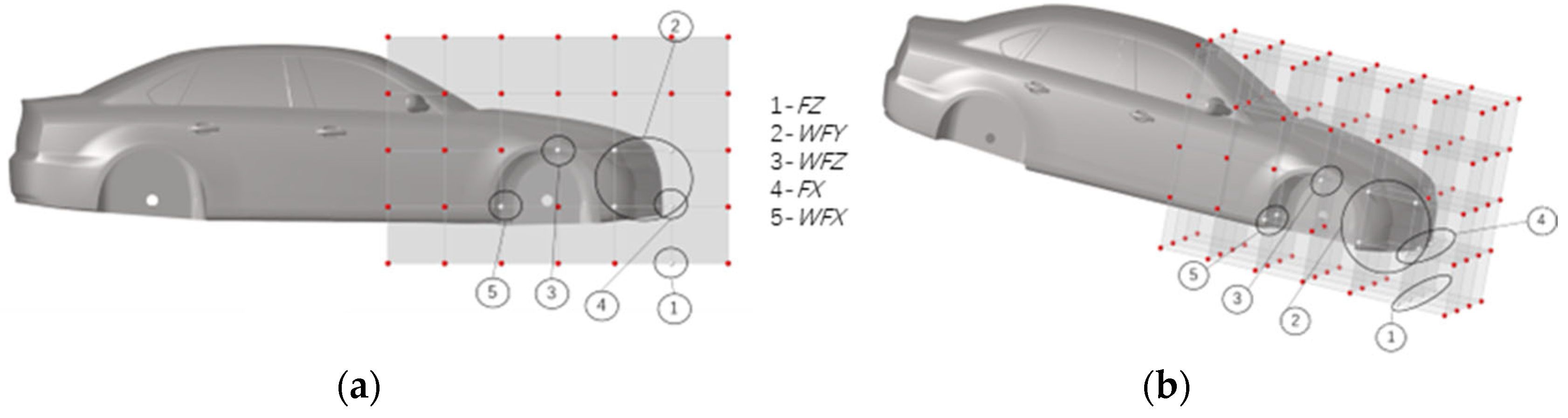
| 1. The height of the front fender from the ground (FZ)32.33.182.184(z) | −0.35 | 0.35 |
| 2. The transverse width of the fender (WFY)69.92.96.102(y) | −0.15 | 0.15 |
| 3. The height of the fender from the ground (WFZ)74.158.75.160(z) | −0.05 | 0.05 |
| 4. The longitudinal length of the front fender (FX)92.90.141.142(x) | −0.1 | 0.1 |
| 5. The longitudinal length of the fender (WFX)80.164(x) | −0.05 | 0.05 |
| No. | FZ/m | WFY/m | WFZ/m | FX/m | WFX/m | Sound Pressure Level/dB | |
|---|---|---|---|---|---|---|---|
| Point 5 | Point 14 | ||||||
| 1 | −0.018 | 0.134 | −0.008 | 0.026 | −0.05 | 99.87 | 105.07 |
| 2 | −0.092 | −0.103 | 0.029 | −0.1 | 0.008 | 103.46 | 102.77 |
| 3 | −0.276 | 0.087 | −0.034 | 0.058 | 0.013 | 103.46 | 102.93 |
| 4 | −0.239 | −0.134 | 0.018 | 0.047 | 0.024 | 99.15 | 104.16 |
| 5 | 0.239 | −0.055 | 0.045 | 0.005 | 0.034 | 96.83 | 100.7 |
| 6 | −0.350 | −0.024 | 0.002 | −0.026 | −0.034 | 97.35 | 100.87 |
| 7 | 0.350 | 0.008 | 0.008 | 0.079 | −0.024 | 99.09 | 103.67 |
| 8 | −0.055 | −0.071 | −0.040 | 0.068 | −0.029 | 96.44 | 104.04 |
| 9 | 0.129 | 0.150 | 0.013 | 0.037 | 0.029 | 94.73 | 105.07 |
| 10 | 0.276 | −0.150 | −0.018 | −0.016 | 0.002 | 109.68 | 105.87 |
| 11 | −0.203 | −0.087 | −0.045 | −0.047 | 0.018 | 101.54 | 105.32 |
| 12 | −0.166 | 0.039 | 0.034 | 0.100 | −0.013 | 98.64 | 104.22 |
| 13 | −0.129 | 0.118 | −0.029 | −0.089 | −0.008 | 97.41 | 102.24 |
| 14 | −0.313 | 0.055 | 0.024 | −0.037 | 0.040 | 97.53 | 101.35 |
| 15 | 0.166 | 0.024 | −0.013 | −0.068 | 0.050 | 98.32 | 104.7 |
| 16 | 0.203 | −0.008 | −0.003 | −0.079 | −0.045 | 124.07 | 104.35 |
| 17 | 0.092 | −0.039 | −0.024 | 0.089 | 0.045 | 97.75 | 105.19 |
| 18 | 0.018 | 0.103 | 0.050 | −0.058 | −0.018 | 96.28 | 102.9 |
| No. | FZ/m | WFY/m | WFZ/m | FX/m | WFX/m | Sound Pressure Level/dB | |
|---|---|---|---|---|---|---|---|
| Point 5 | Point 14 | ||||||
| Original | 0 | 0 | 0 | 0 | 0 | 98.57 | 104.82 |
| Opti | −0.350 | −0.031 | 0.003 | −0.031 | −0.035 | 94.85 | 102.01 |
| Opti CFD | −0.350 | −0.031 | 0.003 | −0.031 | −0.035 | 96.12 | 103.45 |
| Errors/% | - | - | - | - | - | 1.34 | 1.41 |
Disclaimer/Publisher’s Note: The statements, opinions and data contained in all publications are solely those of the individual author(s) and contributor(s) and not of MDPI and/or the editor(s). MDPI and/or the editor(s) disclaim responsibility for any injury to people or property resulting from any ideas, methods, instructions or products referred to in the content. |
© 2024 by the authors. Licensee MDPI, Basel, Switzerland. This article is an open access article distributed under the terms and conditions of the Creative Commons Attribution (CC BY) license (https://creativecommons.org/licenses/by/4.0/).
Share and Cite
Jiao, D.; Zhou, H.; Huang, T.; Zhang, W. Numerical Study on Aerodynamic Noise Reduction in Passenger Car with Fender Shape Optimization. Symmetry 2024, 16, 651. https://doi.org/10.3390/sym16060651
Jiao D, Zhou H, Huang T, Zhang W. Numerical Study on Aerodynamic Noise Reduction in Passenger Car with Fender Shape Optimization. Symmetry. 2024; 16(6):651. https://doi.org/10.3390/sym16060651
Chicago/Turabian StyleJiao, Dongqi, Haichao Zhou, Tinghui Huang, and Wei Zhang. 2024. "Numerical Study on Aerodynamic Noise Reduction in Passenger Car with Fender Shape Optimization" Symmetry 16, no. 6: 651. https://doi.org/10.3390/sym16060651
APA StyleJiao, D., Zhou, H., Huang, T., & Zhang, W. (2024). Numerical Study on Aerodynamic Noise Reduction in Passenger Car with Fender Shape Optimization. Symmetry, 16(6), 651. https://doi.org/10.3390/sym16060651