Abstract
In this article, we consider the statistical analysis of the parameter estimation of the Marshall–Olkin extended generalized extreme value under liner normalization distribution (MO-GEVL) within the context of progressively type-II censored data. The progressively type-II censored data are considered for three specific distribution patterns: fixed, discrete uniform, and binomial random removal. The challenge lies in the computation of maximum likelihood estimations (MLEs), as there is no straightforward analytical solution. The classical numerical methods are considered inadequate for solving the complex MLE equation system, leading to the necessity of employing artificial intelligence algorithms. This article utilizes the genetic algorithm (GA) to overcome this difficulty. This article considers parameter estimation through both maximum likelihood and Bayesian methods. For the MLE, the confidence intervals of the parameters are calculated using the Fisher information matrix. In the Bayesian estimation, the Lindley approximation is applied, considering LINEX loss functions and square error loss, suitable for both non-informative and informative contexts. The effectiveness and applicability of these proposed methods are demonstrated through numerical simulations and practical real-data examples.
1. Introduction
The extreme value theory (EVT) is fundamental to various sectors, including environmental sciences, engineering, finance, insurance, and others. In finance, EVT is especially important for studying the changes in price for many areas, like financial assets or market indices. Forecasting for a better understanding of these extremes is important for effective risk management and strategy formulation. The importance of EVT lies in modeling the distribution tail, which is important in evaluating the risk of rare events. This is especially important in many aspects; it is crucial in market crashes or unexpected increases, where typical financial models may not appropriately capture the risk or possible effects. Ref. [1] is an excellent resource that provides in-depth insights into EVT and its applications to financial data, providing a comprehensive understanding of its methodologies and implications in the financial sector. EVT’s primary goal is to provide a probabilistic description of extreme occurrences within a series of random events. The core concepts of EVT, as originally outlined by [2], form the cornerstone of the conventional EVT framework.
EVT identifies three forms of extreme value distributions: Frechet, Gumbel, and inverse Weibull. The Frechet distribution has an unbounded, hefty upper tail, indicating that it can handle very big numbers. Moreover, it is especially beneficial for modeling data with extreme maxima that are much higher than the average. Meanwhile, the Gumbel distribution is famous for its lighter upper tail, particularly when compared to the Frechet distribution. The Gumbel distribution is frequently used in situations when the distribution of extremes lacks a heavy tail. Due to the inverse Weibull distribution being known to have a finite upper tail, this feature makes it appropriate for simulating situations for values to have a clear upper bound. Generalized extreme value liner distributions (GEVL) is a unified framework that combines these three types of distributions, offering a comprehensive approach for modeling extremes. This versatility makes EVT a powerful tool in statistical analysis, especially in fields where understanding and predicting extreme events is crucial. Several authors have delved into studies concerning GEVL distributions, including [3,4,5,6,7,8] among others.The GEVL probability density function (PDF) and cumulative distribution function (CDF) are given, respectively, as,
and the support of the distribution is
Hence, indicates several parameter sets based on the value. when , suggesting a three-parameter model. However, when approaches zero, , indicating a two-parameter model. is a location parameter, is a scale parameter, and is the shape parameter that affects the distribution’s tail behavior. The values of , whether they be approaching 0, are positive, or are negative, define sub-models representing the Gumbel, Frechét, and Weibull distributions mentioned earlier.
Marshall and Olkin (1997) proposed a technique for modifying any distribution by adding a new parameter, and it is considered a very helpful tool for academics, providing a methodical approach for refining and adapting current distribution models to better suit a wide range of practical applications. Their technology has been widely applied in a variety of industries where an accurate model of data distribution is required. Ref. [9] emphasizes their substantial contribution to statistical theory, especially in extending families of distributions. According to [10], the Marshall–Olkin family of extended distributions is widely applicable and valuable in statistical analysis. They initiated their method by taking a base survival function (SF) and PDF, denoted as and , respectively, to construct a new survival function and PDF as
respectively, where, and , which is known as Marshall and Olkin extension. Many authors utilized the Marshall–Olkin method as an extension to the parent distribution, such as [11,12,13,14].
Because of their robust asymptotic features, maximum likelihood estimation (MLE) and Bayesian approaches have become widely known and used for parameter estimation. MLE treats parameters as fixed but unknown values, which is often useful in estimating measures like means or variances. On the other hand, Bayesian approaches estimate parameters using known prior distributions. This fundamental difference allows Bayesian analysis to incorporate prior knowledge or beliefs about the parameters, making it an exceedingly flexible and powerful tool in statistical inference. For those interested in a deeper understanding of these methodologies and their applications, the work by [15] is an excellent resource.
This paper uses the artificial intelligence algorithm in the estimation process due to the limitation of the traditional numerical method in dealing with complex systems of equations. The genetic algorithms (GAs) fall under the broader category of evolutionary computation. GAs employ mechanisms akin to natural selection. A genetic algorithm (GA) encodes potential solutions to a problem as ’chromosomes,’ which undergo iterative processes of selection, crossing, and mutation. Through these iterations, the population evolves, ideally leading to increasingly optimal solutions. The algorithm’s strength lies in its ability to search through vast and complex solution spaces, making it applicable to a wide variety of problems in optimization and machine learning.
Refs. [16,17] offer deep insights into GAs. Ref. [16] provides a comprehensive overview of GAs, delving into their mechanisms, applications, and theoretical underpinnings. Ref. [17] focuses on the practical applications of GAs, offering insights into how these algorithms can be implemented and optimized for various real data problems.
In many experiments, observing the failure of all units under study can be a challenge due to many constraints, such as time limitations, budgetary restrictions, or other practical limitations. To address this problem, censoring schemes are commonly utilized. Censoring in statistical analysis is a technique primarily utilized in the fields of reliability testing and survival analysis.Censoring allows researchers to make inferences about the entire data set, even for units with unknown failure times. It is particularly useful in many fields, such as reliability engineering, where testing until the failure of all components may be impractical or impossible, and in medical research, where patients may leave a study before its conclusion or the event of interest (like recovery or relapse) has not occurred before the study ends.
The type II progressive censored scheme is a popular censoring strategy for parameter estimation research. Type II progressive censored data is described as follows: Consider an experiment with N items. Only a preset number, designated as n (where ), are observed until they fail. When the first failure donated by occurs, a certain number of items are randomly eliminated from the items . Subsequently, when the second failure occurs, another set of items is randomly eliminated from the remaining items, and this process continues. This process repeats until the nth failure occurs at this point, and the experiment is ended. The type-II progressive censored technique enables researchers to collect and evaluate data without censoring failure times across all objects in the experiment. For more comprehensive information on this scheme, refer to the work by [18]. Also, many others have used type-II progressive censored scheme in their papers, such as [19,20,21,22,23].
This paper’s structure is methodically arranged into sections, beginning with a discussion on the Marshall–Olkin extended generalized extreme value under linear normalization distribution, addressing PDF and CDF along with type-II progressive censoring schemes, in Section 2. It progresses to parameter estimation using type-II progressively censored samples; exploring both point estimates and confidence intervals is discussed in Section 3. In Section 4, Bayesian estimation techniques are detailed, followed by Section 5, which gives the simulation analysis demonstrating theoretical applications. Then, in Section 6, practical applications are exemplified through real data analysis. Finally, Section 7 presents the paper’s conclusions.
2. Marshall–Olkin Extended Generalized Extreme Value under Linear Normalization Distribution and Cases of Type-II Progressive Censored Scheme Considered
2.1. Marshall–Olkin Extended Generalized Extreme Value under Linear Normalization Distribution
Let Marshall–Olkin extended generalized extreme value Under linear normalization distribution. By using Equations (1) and (2) at Equations (4) and (5) to obtain the survival function (SF) and PDF of the Marshall–Olkin extended GEVL (MO-GEVL) contained Marshall–Olkin extended Gambul (MO-Gambul) when and , respectively, are
and
The parameter set , which consists of for and transitions to as approaches zero, plays a critical role in defining the distribution’s characteristics. The influence of and on the distribution’s PDF and CDF shapes is graphically depicted in Figure 1, Figure 2, Figure 3 and Figure 4 to facilitate a deeper understanding of their impacts.
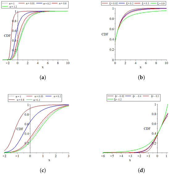
Figure 1.
Plots of the parent distribution GEVL at and the MO-GEVL cumulative function where for certain parameter values. (a) When is random and is fixed where, . (b) when is fixed and is random, where . (c) when is random and is fixed, where . (d) when is fixed and is random, where .
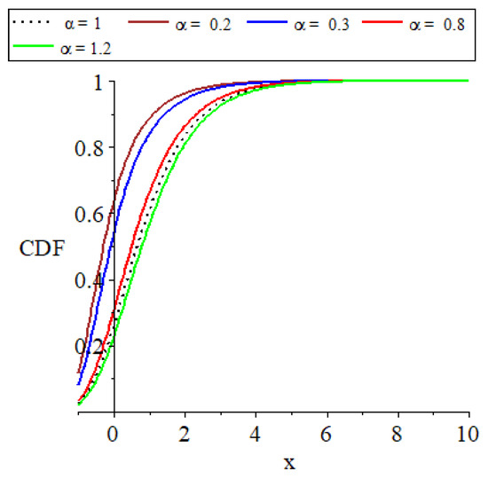
Figure 2.
Plots of the parent distribution GEVL at and the MO-GEVL cumulative function, where and .
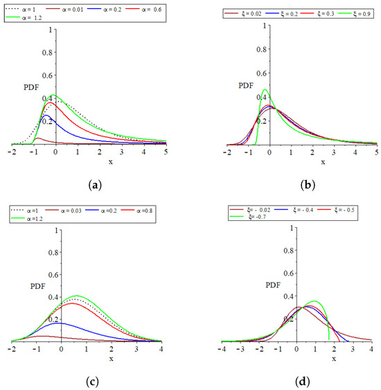
Figure 3.
Plots of the parent distribution GEVL at and the MO-GEVL probability density function where for certain parameter values. (a) When is random and is fixed, where . (b) When is fixed and is random, where . (c) When is random and is fixed, where . (d) When is fixed and is random, where .
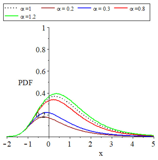
Figure 4.
Plots of the parent distribution GEVL at and the MO-GEVL probability density function where for certain parameter values, where .
Remark 1.
1: Ref [24] is a special case of our paper at .
- 2:
- 3:
- 4:
- The provided plots effectively show the remarkable flexibility of the models introduced.
2.2. Cases of Type-II Progressive Censored Scheme Considered
Assume that is the censoring scheme for the progressively type-II censored ordering data from the MO-GEVL distribution and observed data .
- The first scenario: Fixed Removal Censoring Scheme
In The first scenario, is considered to be predefined set values of the censoring structure.
- The second scenario: Removals With Discrete Uniform Distribution
In this scenario, the censoring scheme is characterized as an independent random variable adhering to a discrete uniform distribution. The joint likelihood function of ℜ is given by,
where
where , , and .
From Equation (9) in Equation (8), the joint distribution of R can be easily obtained as,
It is noticed that Equation (10) is parameter-free; see [25].
- The third scenario: Removals With Binomial Distribution
In this particular scenario, the censoring scheme is modeled as an independent random variable that adheres to binomial distributions, characterized by a specific probability P; see [26]. Then, the joint distribution of is given by
where
where , , for and .
3. Maximum Likelihood Estimation of Parameters and Observed Fisher Information
In the subsequent section, we investigated into the point and interval estimations of the MO-GEVL distribution parameters generated from type-II progressively censored data for the three scenarios explained above. The interval estimate employs observed Fisher information and combines both complete and approximation likelihood equations to establish parameter confidence intervals.
3.1. Maximum Likelihood Estimation of Parameters
To estimate the MO-GEVL distribution parameters based on type-II progressively censored data for all three scenarios discussed above, consider as representing the sequence of failure times arranged in ascending order from a selection of n of N being a pre-established number before initiating the test. When a failure occurs at point i, all units are progressively eliminated from the exam. the joint likelihood function is
- The first scenario:
- The second scenario:
- The third scenario:
Clearly, The maximum likelihood equations (ML equations)for the three scenarios are identical; the only difference is the PDF of the censored scheme . Additionally, in the third scenario, the MLE of P can be identified easily. as
When obtaining the ML equations of parameters by substituting with Equations (6) and (7) at Equation (14), the likelihood function is obtained as
where and . The ML equations of the MO-GEVL and MO-Gumbel distributions could be easily driven by taking the derivative of log of Equation (18) concerning the parameters of , and making them equal to zero. Then, the MLEs of the MO-GEVL distribution are
and
Meanwhile, the ML equations of the MO-Gumbel distribution are
and
Notice:
In type-II progressively censored data, the maximum likelihood estimators (MLEs) for the parameters and are derived by setting the equations from (19) to (22) and from (23) to (25) to zero. The nonlinear characteristics of the likelihood equations Equations (19)–(22) and Equations (23)–(25) are considered a challenge as they do not have a straightforward explicit solution. Given a specific set of a given value , obtaining the maximum likelihood estimators of parameters involves solving these complex equations, which may not be available by classical techniques. Artificial intelligence algorithms are used to discover the optimum probability estimators based on observable data and equations. We used (GA), a popular AI technique that optimizes MLE using type-II progressively censored data. GA is explained in detail on the following website, https://cran.r-project.org/web/packages/GA/vignettes/GA.html#:~:text=The%20R%20package%20GA%20provides,case%2C%20whether%20constrained%20or%20not, accessed on 1 March 2024.
3.2. Observed Fisher Information and Approximate Confidence Interval Concerning the Distribution of the Censoring Scheme
The observed Fisher information is determined by utilizing both the complete and approximate likelihood equations. This approach enables a thorough evaluation of the precision of the parameter estimates derived from the data, providing critical insights into the variability of the estimation process in statistical analysis. Monte Carlo simulations are used to systematically analyze the performance of pivotal quantities. For sufficiently high sample sizes (i.e., > 0), we can create approximate confidence ranges for the three scenarios previously discussed. Confidence intervals offer insights into parameter estimations’ precision and statistical significance across different contexts.
3.2.1. Observed Fisher Information Corresponding
Under the presumption of censoring scheme distribution, the Fisher information matrix, based on log-likelihood functions given in Equation (18) for scenarios 1 and 2, obtained using and if and , respectively, is
and
Meanwhile, for The third scenario, the fisher information matrix and for and , respectively, is obtained as
and
where and are the log of likelihood function of Equation (18) for and , respectively. Then, the partial derivatives are given by
,
where and .
3.2.2. The Asymptotic Confidence Interval
The variance-covariance matrix can be obtained by computing the inverse of matrices (, and ), depending on the scenario under investigation. According to [27], the asymptotic distribution of vector of parameter for the scenarios 1, 2, and 3 adheres to the normal distribution . The asymptotic confidence interval for parameters at significance level r can be found by
where represents the variance–covariance matrix.
4. Bayesian Estimation
We discuss the Bayesian estimation for the MO-GEVL distribution parameters under the three cases proposed in this section. We combine both the observed sample data and the prior knowledge about the sample distribution. Combining the prior probabilities and available information on the population distribution provides a more subjective and informed perspective on unknown parameters. We next explore parameter estimation using Bayesian methods, focusing on two loss functions: square loss and LINEX loss. Our analysis covers two different scenarios: one with informative priors, which rely on specific prior knowledge, and another with non-informative priors, which assume minimal prior information. By integrating these loss functions and types of prior information, we thoroughly examine parameter estimation.
Informative priors. Assume that the unknown parameters in every scenario investigated are independent of one another. The approach of selecting parameter priors for informative cases depends on the parameter validation region, as introduced by [28,29]. So, we considered the priors PDF of the parameters follow an exponential distribution with the hyper-parameters , while the random variable P follows a beta distribution with parameters . Then, the prior PDF of the parameters are
and
where is the beta function. The hyperparameters (, , if ) are estimated by the same method given in [30]. Then, the joint PDF of hyperparameters for MO-GEVL could be written as
where if and if . It is easy to obtain the joint PDF of hyperparameters for MO-Gambul by putting into Equation (50) equal to 0.
Non-informative prior. For this scenario all parameters prior PDFs are assumed to be equal to 1.
According to the informative prior, the posterior PDFs of MO-GEVL for and , respectively, are given by,
where and . Then, the informative Bayesian estimation under the SELF and LINEX loss functions (see, [31]) are given respectively by
where is a shape parameter, in which its negative value provides more weight to underestimation compared with the overestimation, while for it’s small or large values, the LINEX loss [] function is almost symmetric (see [32]).
Meanwhile, for non-informative priors, the posterior PDFs are given by
where and .
The Bayesianestimation of parameters for MO-GEVL using the SELF and LINEX for the informative prior function. by
The systems of equations are presented as Equations (53), (54), (57) and (58) do not have analytical solutions, so it is necessary to use numerical methods for their solution. Among these methods, Lindley’s approximation technique stands out as a popular choice for Bayesian estimation. We will explore this method in detail in the subsequent subsection.
Lindley’s Approximation Method
Lindley’s approximation is a simple technique for approximating the ratio of integrals in systems of equations (Equations (53), (54), (57) and (58)). Other methods, such as the Markov Chain Monte Carlo method and Gibbs sampler, are also used. the easily analytical approach of Lindley’s approximation makes it a popular choice for solving problems among the other analytical approach. The method typically involves expanding the log-likelihood and the log-prior around a suitable point, such as the mode of the posterior distribution, and then approximating the integral using this expansion. This approach is particularly useful when the exact computation of the integral is challenging. Lindley’s approximation provides a way to estimate the expected value of under the posterior distribution, which is crucial in Bayesian analysis for making inferences about the parameters based on the observed data. Below is the Lindley approximation of
In this context, is a vector representing a set of parameters. The function is defined as a function of these parameters.
where ,, , , and is equal to the variance covariance matrix. All partial derivatives are evaluated at the maximum likelihood estimation of parameters. For more details, see [33].
5. Simulation
A Monte Carlo simulation is performed in this section to compare the performance of various estimator parameters discussed in the preceding sections. This simulation offers a comprehensive evaluation of different estimation methods on their effectiveness in parameter estimation. The simulation involves generating 1000 samples for two different sample sizes 100 and 200 for a variable X. In this analysis, the maximum likelihood estimator (MLE) for the parameters is evaluated compared with the Bayesian estimators within the framework of two distinct loss functions: the squared error loss and the linear exponential (LINEX) loss function. The reason for this comparison is to provide insight into their relative performance and suitability for statistical analysis. Moreover, we explore Bayesian estimation using Lindley’s method for the informative and non-informative priors. For the informative priors, the hyperparameters are determined following the approach initiated by [30] and subsequently employed by [34]. Additionally, an approximate confidence interval for the parameters is calculated, offering a comprehensive statistical analysis based on the established methodologies. The LINEX loss function is evaluated for three different values of , as shown in Table 1 and Table 2. Table 3 introduces the lower bound (LB), upper bound (UB), and length of the confidence interval (LC). All calculations are performed using the R programming language. The estimators are evaluated under three different scenarios of random removals, with censoring schemes involving a 10% elimination from the sample size. Moreover, fixed random removal is executed either at the beginning or the end of the sample. For details on the algorithm for generating progressive censoring of type-II, see [18].

Table 1.
The bias and MSE for the MLE and Bayesian estimation of parameters for informative and non-informative priors under the SELF(sq) LINEX loss function at () for n = 100,200 for The first scenario.
Table 2.
The bias and MSE for the MLE and Bayesian estimation of parameters for informative and non-informative priors under the SELF(sq) LINEX loss function at () for for The second scenario and 3.
Table 3.
The 95% confidence intervals of parameters of MO-GEVL under the three cases of censoring schemes.
From Table 1, the informative Bayesian estimation gives a small bias and MSE compared with the non-informative Bayesian estimation. Bayesian estimation utilizing the LINEX loss function tends to give better outcomes in terms of bias and mean squared error (MSE) when compared with the squared error loss function. This advantage is particularly noted when the parameter holds a negative value, emphasizing a greater penalty for underestimation than overestimation. The LINEX loss function approaches symmetry for extremely small or large values of , as detailed in the study by [32]. This finding underscores the effectiveness of the LINEX loss function in various estimation scenarios.
Furthermore, in the first situation, eliminating at the beginning provides a more accurate estimate of bias and MSE compared to eliminating at the end. In terms of the sensitivity of GA for the sample size, we find that the behavior is consistent for both small and high sample sizes. Furthermore, MLE provides better bias than Bayesian estimate. In Table 2, it is apparent that the confidence interval demonstrates that as sample size grows, we obtain a better estimate in terms of shorter intervals encompassing the real value. The Lindley approximation for the second scenario fails to effectively estimate parameters for a sample size of 100. However, for , the estimation improves in terms of bias and MSE.
6. Real Data Example
In this section, we apply the discussed algorithms using actual real data, with a focus on extreme weather events. Extreme weather phenomena, including heatwaves, droughts, and wildfires, are often associated with high temperatures. It is important to recognize that such excessively high temperatures can lead to significant health risks and heat-related illnesses.
Given the recent global crisis triggered by an unexpected rise in temperature levels, understanding historical temperature extremes for each country has become vital. This information is crucial for mitigating the impact of catastrophic events caused by these temperature increases. It also helps in assessing the frequency, severity, and consequences of such events, thereby aiding in the development of more effective strategies for preparedness and response.
For practical demonstration, we analyze real data sets representing the temperatures in Egypt from 1999 to 2023. These data was sourced from https://www.ogimet.com/home.phtml.en, accessed on 12 May 2024.
Table 4 provides basic statistics for this data set, including mean, variance, median, and other relevant measures. This statistical analysis offers insights into the temperature trends in Egypt over the specified period, contributing to a broader understanding of the impacts of rising temperatures on a national scale.
Table 4.
The basic statistics of extreme temperatures in Celsius for the Egypt data set.
In Table 5, these data sets are fitted to both GEVL and MO-GEVL by using computationally intensive ways of comparing model fits like the Kolmogorov–Smirnov(K–S) goodness of fit test at the level of significance of , , Akaike information criterion (AIC) [35], and Bayesian information criterion (BIC) [36].
Table 5.
The values of K-S, , (AIC), and BIC for both GEVL and MO-GEVL distributions.
Moreover, Figure 5 shows the empirical data and fitted cumulative distribution function plot for GEVL and MO-GEVL.
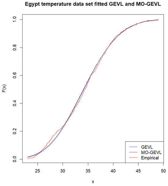
Figure 5.
The empirical and fitted cumulative distribution function plot for GEVL and MO-GEVL.
The results in Table 5 for that data set show that both (GEVL–MO-GEVL) distributions give a good fit for these data, while MO-GEVL gives a better fit than GEVL in terms of lower indicators (KS,, AIC, and BIC). Moreover, the Figure 5 indicates that the MO-GEVL distribution provides a better reasonable fit than GEVL.
In Table 6, we introduce the maximum likelihood estimate and Bayes estimates of MO-GEVL parameters considered in the above sections for the three cases of elimination, considered using a GA.
Table 6.
MLE and Bayes estimates for , where X represents the temperature of Egypt and Y represents the temperature of Queensland (Australia).
7. Conclusions
This study focuses on parameter estimation for variables following the Marshall–Olkin extended generalized extreme value distribution (MO-GEVL) within the framework of type-II progressive censoring. This methodological approach aims to enhance the accuracy of statistical inferences drawn from censored data sets, providing significant insights into the distribution’s characteristics and behavior under specified conditions.
We utilize artificial intelligence, specifically genetic algorithms (GAs), for estimating maximum likelihood estimation (MLE) parameters. Additionally, a Bayesian estimation of parameters is examined under two types of loss, functions-symmetric and asymmetric, considering both informative and non-informative priors.
We also use progressive censoring type-II under three different scenarios of elimination: fixed, discrete uniform, and binomial, with a elimination from the sample size. Within the fixed random removal censoring scheme, we consider two specific cases: elimination at the beginning and at the end of the sample.
A Monte Carlo simulation is conducted to compare the performance of various estimators for the GEVL distribution parameters using Lindley’s method. The simulation results show that informative Bayesian estimation yields results very close to non-informative Bayesian estimation in terms of bias and mean squared error (MSE), but it is still better than the non-informative case. Furthermore, Bayesian estimation under the LINEX loss function shows comparable results with the SELF-loss function regarding both Bias and MSE. It is noted that a negative value of in the LINEX loss function places more emphasis on underestimation compared with overestimation. For extreme (small or large) values of , the LINEX loss function tends to be almost symmetric, as illustrated in Table 1.
For the first case of elimination, removing samples at the beginning provides better estimates in terms of bias and MSE than elimination at the end. In terms of the sensitivity of estimates to sample size, the GA’s performance is consistent across both smaller and larger sample sizes. Moreover, MLE tends to offer better Bias compared with Bayesian estimation. As illustrated in Table 3, we noticed that as sample sizes increase, we receive more accurate estimates of the confidence interval in terms of a smaller interval length that contains both the true and estimated values of the parameters.
Author Contributions
Conceptualization, R.A.E.-W.A., S.W.S. and T.R.; methodology, R.A.E.-W.A., S.W.S. and T.R.; software, R.A.E.-W.A., S.W.S. and T.R.; validation, R.A.E.-W.A., S.W.S. and T.R.; formal analysis, R.A.E.-W.A., S.W.S. and T.R.; investigation, R.A.E.-W.A., S.W.S. and T.R.; resources, R.A.E.-W.A., S.W.S. and T.R.; data curation, R.A.E.-W.A., S.W.S. and T.R.; writing—original draft preparation, R.A.E.-W.A., S.W.S. and T.R.; writing—review and editing, R.A.E.-W.A., S.W.S. and T.R.; visualization, R.A.E.-W.A., S.W.S. and T.R.; supervision, R.A.E.-W.A., S.W.S. and T.R.; project administration, R.A.E.-W.A., S.W.S. and T.R.; funding acquisition, T.R. All authors have read and agreed to the published version of the manuscript.
Funding
This research was funded by the Deanship of Graduate Studies and Scientific Research at Qassim University, Saudi Arabia.
Data Availability Statement
Data are contained within the article.
Acknowledgments
The Researchers would like to thank the Deanship of Graduate Studies and Scientific Research at Qassim University for financial support (QU-APC-2024-9/1).
Conflicts of Interest
The authors declare no conflicts of interest.
References
- Gilli, M.; Këllezi, E. An application of extreme value theory for measuring financial risk. Comput. Econ. 2006, 27, 207–228. [Google Scholar] [CrossRef]
- Fisher, R.A.; Tippett, L.H.C. Limiting forms of the frequency distribution of the largest or smallest member of a sample. In Mathematical Proceedings of the Cambridge Philosophical Society; Cambridge University Press: Cambridge, UK, 1928; Volume 24, pp. 180–190. [Google Scholar]
- Bali, T.G. The generalized extreme value distribution. Econ. Lett. 2003, 79, 423–427. [Google Scholar] [CrossRef]
- Hosking, J.R.M.; Wallis, J.R.; Wood, E.F. Estimation of the generalized extreme-value distribution by the method of probability-weighted moments. Technometrics 1985, 27, 251–261. [Google Scholar] [CrossRef]
- Bertin, E.; Clusel, M. Generalized extreme value statistics and sum of correlated variables. J. Phys. A Math. Gen. 2006, 39, 7607. [Google Scholar] [CrossRef]
- Hu, X.; Fang, G.; Yang, J.; Zhao, L.; Ge, Y. Simplified models for uncertainty quantification of extreme events using Monte Carlo technique. Reliab. Eng. Syst. Saf. 2023, 230, 108935. [Google Scholar] [CrossRef]
- Ali, Y.; Haque, M.M.; Mannering, F. A Bayesian generalised extreme value model to estimate real-time pedestrian crash risks at signalised intersections using artificial intelligence-based video analytics. Anal. Methods Accid. Res. 2023, 38, 100264. [Google Scholar] [CrossRef]
- Lovell, C.C.; Harrison, I.; Harikane, Y.; Tacchella, S.; Wilkins, S.M. Extreme value statistics of the halo and stellar mass distributions at high redshift: Are JWST results in tension with ΛCDM? Mon. Not. R. Astron. Soc. 2023, 518, 2511–2520. [Google Scholar] [CrossRef]
- Marshall, A.W.; Olkin, I. A new method for adding a parameter to a family of distributions with application to the exponential and Weibull families. Biometrika 1997, 84, 641–652. [Google Scholar] [CrossRef]
- Jose, K. Marshall-Olkin family of distributions and their applications in reliability theory, time series modeling and stress-strength analysis. In Proceedings of the 58th World Statistical Congress, Dublin, Ireland, 21–26 August 2011; Volume 201, pp. 3918–3923. [Google Scholar]
- Obulezi, O.J.; Anabike, I.C.; Oyo, O.G.; Igbokwe, C.; Etaga, H. Marshall-Olkin Chris-Jerry distribution and its applications. Int. J. Innov. Sci. Res. Technol. 2023, 8, 522–533. [Google Scholar]
- Ozkan, E.; Golbasi Simsek, G. Generalized Marshall-Olkin exponentiated exponential distribution: Properties and applications. PLoS ONE 2023, 18, e0280349. [Google Scholar] [CrossRef]
- Niyoyunguruza, A.; Odongo, L.O.; Nyarige, E.; Habineza, A.; Muse, A.H. Marshall-Olkin Exponentiated Frechet Distribution. J. Data Anal. Inf. Process. 2023, 11, 262–292. [Google Scholar]
- Alsadat, N.; Nagarjuna, V.B.; Hassan, A.S.; Elgarhy, M.; Ahmad, H.; Almetwally, E.M. Marshall–Olkin Weibull–Burr XII distribution with application to physics data. AIP Adv. 2023, 13, 095325. [Google Scholar] [CrossRef]
- Phoong, S.Y.; Ismail, M.T. A comparison between Bayesian and maximum likelihood estimations in estimating finite mixture model for financial data. Sains Malays. 2015, 44, 1033–1039. [Google Scholar] [CrossRef]
- Haldurai, L.; Madhubala, T.; Rajalakshmi, R. A study on genetic algorithm and its applications. Int. J. Comput. Sci. Eng 2016, 4, 139–143. [Google Scholar]
- Scrucca, L. GA: A package for genetic algorithms in R. J. Stat. Softw. 2013, 53, 1–37. [Google Scholar] [CrossRef]
- Balakrishnan, N.; Balakrishnan, N.; Aggarwala, R. Progressive Censoring: Theory, Methods, and Applications; Springer Science & Business Media: Berlin/Heidelberg, Germany, 2000; pp. 1221–1253. [Google Scholar] [CrossRef]
- Khalifa, E.H.; Ramadan, D.A.; Alqifari, H.N.; El-Desouky, B.S. Bayesian Inference for Inverse Power Exponentiated Pareto Distribution Using Progressive Type-II Censoring with Application to Flood-Level Data Analysis. Symmetry 2024, 16, 309. [Google Scholar] [CrossRef]
- El-Morshedy, M.; El-Sagheer, R.M.; El-Essawy, S.H.; Alqahtani, K.M.; El-Dawoody, M.; Eliwa, M.S. One-and Two-Sample Predictions Based on Progressively Type-II Censored Carbon Fibres Data Utilizing a Probability Model. Comput. Intell. Neurosci. 2022, 2022, 6416806. [Google Scholar] [CrossRef] [PubMed]
- Eliwa, M.S.; Ahmed, E.A. Reliability analysis of constant partially accelerated life tests under progressive first failure type-II censored data from Lomax model: EM and MCMC algorithms. AIMS Math. 2023, 8, 29–60. [Google Scholar] [CrossRef]
- EL-Sagheer, R.M.; El-Morshedy, M.; Al-Essa, L.A.; Alqahtani, K.M.; Eliwa, M.S. The Process Capability Index of Pareto Model under Progressive Type-II Censoring: Various Bayesian and Bootstrap Algorithms for Asymmetric Data. Symmetry 2023, 15, 879. [Google Scholar] [CrossRef]
- EL-Sagheer, R.M.; Eliwa, M.S.; El-Morshedy, M.; Al-Essa, L.A.; Al-Bossly, A.; Abd-El-Monem, A. Analysis of the Stress–Strength Model Using Uniform Truncated Negative Binomial Distribution under Progressive Type-II Censoring. Axioms 2023, 12, 949. [Google Scholar] [CrossRef]
- Attwa, R.; Sadk, S.; Aljohani, H. Investigation the generalized extreme value under liner distribution parameters for progressive type-II censoring by using optimization algorithms. AIMS Math 2024, 9, 15276–15302. [Google Scholar] [CrossRef]
- Wu, S.J.; Chang, C.T. Inference in the Pareto distribution based on progressive type II censoring with random removals. J. Appl. Stat. 2003, 30, 163–172. [Google Scholar] [CrossRef]
- Ghahramani, M.; Sharafi, M.; Hashemi, R. Analysis of the progressively Type-II right censored data with dependent random removals. J. Stat. Comput. Simul. 2020, 90, 1001–1021. [Google Scholar] [CrossRef]
- Lawless, J.F. Statistical Models and Methods for Lifetime Data; John Wiley & Sons: Hoboken, NJ, USA, 2011. [Google Scholar]
- Mokhlis, N.A. Reliability of a Stress-Strength Model with Burr Type III Distributions. Commun. Stat.-Theory Methods 2014, 34, 1643–1657. [Google Scholar] [CrossRef]
- Mokhlis, N.A.; Khames, S.K.; Sadk, S.W. Estimation of Stress-Strength Reliability for Marshall-Olkin Extended Weibull Family Based on Type-II Progressive Censoring. J. Stat. Appl. Probab. 2021, 10, 385–396. [Google Scholar]
- Ahn, S.E.; Park, C.; Kim, H. Hazard rate estimation of a mixture model with censored lifetimes. Stoch. Environ. Res. Risk Assess. 2007, 21, 711–716. [Google Scholar] [CrossRef]
- Tse, C.; Yuen, H. Statistical analysis of Weibull distributed lifetime data under type II progressive censoring with binomial removals. J. Appl. Stat. 2000, 27, 1033–1043. [Google Scholar] [CrossRef]
- Khatun, N.; Matin, M.A. A study on LINEX loss function with different estimating methods. Open J. Stat. 2020, 10, 52. [Google Scholar] [CrossRef]
- Lindley, D.V. Approximate bayesian methods. Trab. Estadística Y Investig. Oper. 1980, 31, 223–245. [Google Scholar] [CrossRef]
- Ali, S.; Aslam, M. Choice of suitable informative prior for the scale parameter of mixture of Laplace distribution using type-I censoring scheme under different loss function. Electron. J. Appl. Stat. Anal. 2013, 6, 32–56. [Google Scholar] [CrossRef]
- Akaike, H. On Entropy Maximization Principle. In Applications of Statistics; Krishnaiah, P.R., Ed.; Scientific Research Publishing Inc.: Amsterdam, The Netherland, 1977; Available online: https://www.scirp.org/reference/referencespapers?referenceid=2053767 (accessed on 1 March 2024).
- Wright, B.D.; Stone, M.H. Best Test Design: Rasch Measurement; Mesa Press: Chicago, IL, USA, 1979; Available online: https://www.scirp.org/reference/referencespapers?referenceid=1646017 (accessed on 1 March 2024).
Disclaimer/Publisher’s Note: The statements, opinions and data contained in all publications are solely those of the individual author(s) and contributor(s) and not of MDPI and/or the editor(s). MDPI and/or the editor(s) disclaim responsibility for any injury to people or property resulting from any ideas, methods, instructions or products referred to in the content. |
© 2024 by the authors. Licensee MDPI, Basel, Switzerland. This article is an open access article distributed under the terms and conditions of the Creative Commons Attribution (CC BY) license (https://creativecommons.org/licenses/by/4.0/).