Abstract
This study examines the behavior of single-walled carbon nanotubes (SWCNTs) suspended in a water-based ionic solution, driven by the combined mechanisms of electroosmosis and peristalsis through ciliated media. The inclusion of nanoparticles in ionic fluid expands the range of potential applications and allows for the tailoring of properties to suit specific needs. This interaction between ionic fluids and nanomaterials results in advancements in various fields, including energy storage, electronics, biomedical engineering, and environmental remediation. The analysis investigates the influence of a transverse magnetic field, thermal radiation, and mixed convection acting on the channel walls. The novel physical outcomes include enhanced propulsion efficiency due to SWCNTs, understanding the influence of thermal radiation on fluid behavior and heat exchange, elucidation of the interactions between SWCNTs and the nanofluid, and recognizing implications for microfluidics and biomedical engineering. The Poisson–Boltzmann ionic distribution is linearized using the modified Debye–Hückel approximation. By employing real-world approximations, the governing equations are simplified using long-wavelength and low-Reynolds-number approximation. Conducting sensitivity analyses or exploring the impact of higher-order corrections on the model’s predictions in recent literature might alter the results significantly. This acknowledges the complexities of the modeling process and sets the groundwork for further enhancement and investigation. The resulting nonlinear system of equations is solved through regular perturbation techniques, and graphical representations showcase the variation in significant physical parameters. This study also discusses pumping and trapping phenomena in the context of relevant parameters.
1. Introduction
Electroosmosis involves the motion induced by an electric field, where the electrolytic solution moves in relation to the pipe due to an externally applied electric field. The connection between electrokinetic effects and the electric double layer (EDL) has been explored. The initial discovery of electrokinetic effects dates back to 1890 when Reuss conducted experimental studies on porous clays [1]. Electroosmosis [2], a mechanism of electrokinetics, refers to the osmotic movement of molecules/liquids from a less concentrated solution to a more concentrated solution under the influence of an electric field. It explores the interrelation between the motion of aqueous solutions/particles and electroosmotic/electrophoretic forces. Electroosmosis has been a widely explored area of research due to its reliability in microdevices and nanodevices. Recent studies have investigated the significance of electroosmosis in various fields such as industry, biochemistry, and medicine [3]. Its practical uses encompass drug delivery [4], DNA analysis/sequencing systems [5], and the development of biochemical agent detection sensors integrated into microchips. A natural transport process called peristalsis [6,7] utilizes consecutive muscle contraction and relaxation to deal with physiological transport problems. Saleem et al. [8] investigated the peristaltic movement of compressible Jeffrey fluid through a porous channel while being subjected to the influence of a magnetic field.
Exploring peristalsis and electroosmosis concurrently [9] introduces a novel dimension to biomicrofluidics, enabling the study of physiological flows under the influence of external electric fields. Inspired by biomicrofluidics applications integrating peristalsis and electroosmosis, a series of mathematical models [10] have been devised to investigate the alterations in peristaltic transport phenomena induced by electroosmosis. Ranjit and Shit analyzed electroosmotic flow propelled by peristaltic pumping, considering entropy generation [11]. Akram et al. [12] explored Sisko fluid in this context. Ranjit et al. [13] studied the transport of ionic liquid within a porous microchannel, while Bhatti et al. performed a computational analysis of heat and mass transfer in two-phase flow [14]. Additionally, Prakash et al. [15] examined the behavior of ionic nanoliquids in a biomicrofluidics channel, and Tripathi et al. [16] investigated a non-Newtonian Jeffrey fluid in an asymmetric setting. Prakash et al. [17] also conducted a heat transfer analysis in blood flow, and Kattamreddy et al. [18] included thermal analysis of Casson fluids. Akram et al. [19] presented a thermal analysis of Sutterby nanofluids, while Noreen and Ain analyzed entropy generation in porous media [20].
Nanoparticles, measuring around 100 nm in size, are dispersed within a base fluid to create nanofluids. These fluids consist of solid nanoparticles suspended in a base fluid, resulting in enhanced thermal conductivity. Nanoparticles find rapid applications in various industries such as biomedicine, heating and cooling systems, fuel cells, and food processing. The term “nanofluid” was coined by Choi [21]. The inclusion of nanoparticles improves the thermal properties of the base fluid. The homogeneous flow model, initially introduced by Tiwari and Das [22], represents the single-phase nanofluid model.
Cilia are hair-like cellular structures that extend from the cell body into the fluid surrounding the cell. Every cell in the human body contains cilia. Cilia have many functions in various tissues in respiratory tracts, kidneys, oviducts, lungs, sperm, brains, and embryos. In 1962, Sleigh [23] discussed the structure of flagella and cilia and the behavior of metachronal waves. He pointed out the primary influence of ciliary transportation on biological systems. The two types of cilia are motile and non-motile. Motile cilia are typically found on the surfaces of certain types of cells. They can be found in the brain and transport the cerebrospinal fluid within the ventricular system to maintain and nourish brain homeostasis; in the respiratory tract, where they help move mucus and foreign particles out of the airways; in the female reproductive tract to aid in moving eggs along the fallopian tubes; and in the male reproductive tract to help propel sperm. Non-motile cilia can be found in various tissues and organs, including the kidney, eye, brain, and sensory organs. In the eye, they are located inside the retina’s light-sensitive cells (photoreceptors). In kidney collecting ducts and tubules, the function of these cilia is to identify the fluid flow that assists kidney cells in stabilizing their proper procedure of cell division. Cilia development and its function are explained in detail in [24,25]. In the adult human body, the airways, reproductive tracts, and particular brain regions are very abundant in epithelial cells containing motile cilia [26]. Motile cilia play a crucial role in these tissues in the cleaning of mucosa (airways), transportation of oocytes (fallopian tubes), and cerebrospinal fluid circulation (brain) [27]. Maiti et al. [28] discussed the motion of fluid with rheological properties inside a tube induced by a metachronal wave of cilia. Asha and Namrata [29] investigated the synovial issues of ciliary peristalsis. A few core studies on the topic under investigation can be seen in [30,31,32,33,34,35,36,37,38,39,40,41].
The concentration of SWCNTs in nanofluids significantly influences their properties and performance in various applications, including thermal conductivity, mechanical properties, electrical conductivity, optical properties, and potential applications. Numerous research studies have investigated the effects of SWCNT concentration on nanofluid behavior, providing valuable insights into the design and optimization of SWCNT-based nanofluids for specific applications. Choi et al. [42] discussed the unexpected boost in thermal conductivity in suspensions containing nanotubes. Kam et al. [43] explored the multifunctional capabilities of carbon nanotubes as biological transporters and near-infrared agents for targeted cancer cell eradication.
The present study provides a comprehensive analysis of thermal radiation effects on the electroosmotic propulsion of an ionic nanofluid interacting with SWCNTs in ciliated channels. It also enhances our knowledge about complex fluid flow and heat transfer phenomena and has various applications in nanotechnology and biomedical engineering. From the literature survey, it is noticed that different studies are available on cilia-driven flows. Still, the effects of electroosmotic forces in different ciliated channels saturated by non-Newtonian nanofluids are not yet available in the existing literature. To fill this gap, the cilia-driven flow of non-Newtonian fluid under the influence of electroosmotic forces is investigated in this research work.
Future research could focus on conducting experimental studies to validate theoretical models, exploring different nanoparticles, studying the impact of biological variability in ciliated channels, and investigating complex thermal dynamics.
2. Mathematical Formulation
In this study, we will investigate the flow characteristics of an electrically conducting ionic nanofluid, based on water and incorporating single-walled carbon nanotubes (SWCNTs), within a ciliated channel. A combination of peristalsis and electroosmosis drives the fluid flow. An external electric field applied across the electric double layer (EDL) in the axial direction generates electroosmotic forces. The analysis includes the effects of mixed convection and viscous dissipation. Additionally, we examine the impact of thermal radiation, with the radiated heat flux term defined by the Rosseland approximation. A constant magnetic field strength B0 is applied in the transverse direction.
The mathematical model for the flow regime is expressed in [44] as
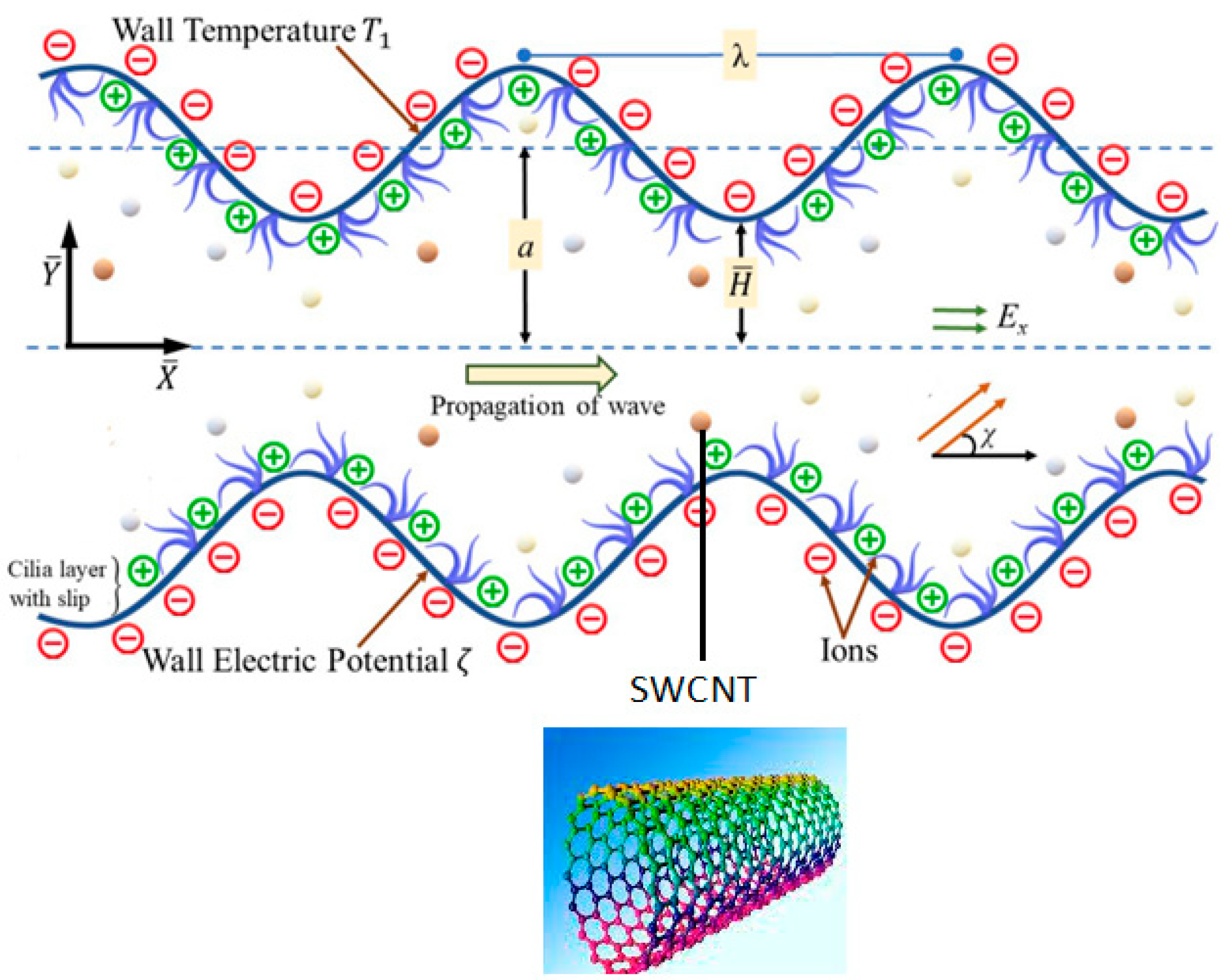
In which “d” is the half-width of the channel, whereas “a” represents the amplitude of sinusoidal waves as shown in Figure 1.

Figure 1.
Geometry of the problem.
The activity of cilia in elliptical tracks is mathematically configured in [45] as
where L is the total width of the channel from the centerline, λ is the wavelength, is the wave speed, and ε is a non-dimensional measure with respect to mean width a. The cilia tips are assumed to move in elliptical paths, such that the horizontal position of the cilia tips can be expressed mathematically as
where the reference position of the particle is while α symbolizes the eccentricity of the elliptical motion. If the no-slip condition is applied to the walls of the channel, then the velocities imparted to the fluid particles remain same as those of the cilia tips.
Further, this cilia activity takes some horizontal plus vertical velocities [46] given below:
3. Governing Equations
The constitutive equations for the current flow problem, under the specified flow conditions, are derived as [47]
where
In this context, represents the radiative heat flux, and it is defined using the Rosseland approximation. It is assumed that the heat flux predominantly influences the direction alone, as indicated in reference [48]:
where , (ργ)nf, σ, ρnf, ρe, , τ, μnf and σnf represents pressure, effective thermal expansion of nanofluid, electric conductivity, effective density of nanofluid, charge number density, electrokinetic body forces in x and y directions, stress tensor, the effective viscosity of nanoliquid, and effective thermal diffusivity of nanoliquid, respectively. The effective thermal conductivity of a carbon nanotube suspension is characterized by the Xue model. The resultant effective properties of SWCNT–water nanofluid are specified in [49].
Here, , , and and Φ represents the density of water, density of single-walled carbon nanotubes, the thermal conductivity of water and single-walled carbon nanotubes, and volume fraction of single-walled carbon nanotubes, respectively.
The Poisson equation is employed to define the electric potential φ generated across the electric double layer (EDL), as indicated in [50]:
where ρe denotes the electric charge number density given by
In this context, denotes electric charge, while n+ and n− represent anions and cations with a bulk concentration of and charge balance z for ionic species. The distribution of ions in the fluid is elucidated by utilizing the Nernst–Planck equation
where, D, , and kB define ionic diffusivity, mean temperature of the ionic solution, and Boltzmann constant.
The transformations used to transform the laboratory frame () to wave frame () are as follows:
To simplify this analysis, we introduce the following dimensionless quantities:
where Pr, δ, θ, U, k, Re, Rd, Gr, Ec, Br, and M represent Prandtl number, wave number, dimensionless temperature, Helmholtz–Smoluchowski velocity, Debye length parameter, Reynolds number, radiation parameter, Grashof number, Eckert number, Brinkman number, and Hartmann number, respectively.
The current problem can be notably simplified by employing the stream function in the following manner:
By substituting Equations (16)–(18) into Equations (6)–(9) and Equations (13)–(15) and applying the long-wavelength and low-Reynolds-number approximation, we derive the following simplified system of equations:
By applying suitable boundary conditions to Equation (23), the resultant expression is as follows:
The Poisson–Boltzmann paradigm is derived by combining Equations (22) and (24).
The Debye–Hückel approximation principle, assuming a lower zeta potential across the electric double layer (EDL), can be applied to simplify the given equation as follows:
Equation (26) is integrated directly while applying the following boundary conditions:
And the resultant electric potential function is expressed as
By incorporating Equation (28) into Equations (19)–(21), we obtain
The associated boundary slip conditions are
The dimensionless flow rate F is expressed as
where Q represents the mean flow rate.
The heat transfer rate can be determined as
4. Solution Procedure
The system of Equations (29)–(33) arises from the mathematical formulation and simplification of the problem, presenting a nonlinear nature that prohibits exact solution. Employing a regular perturbation method allows a reduction in nonlinearity in the mentioned system, facilitating the derivation of an approximate analytical solution. To achieve this, a series expansion of the relevant flow variables around a small Brinkman number is undertaken:
Truncating these series up to O(Br2) only and inserting the above expressions into Equations (29) and (30) and boundary conditions (31)–(33) yield the following zeroth- and first-order systems:
4.1. Zeroth-Order System
4.2. First-Order System
Utilizing the mathematical software Mathematica Version 10, we independently solve the systems of zeroth- and first-order equations to attain an exact solution. The solutions for the stream function, temperature, velocity, and pressure gradient are presented below.
The constants obtained in routine calculations are given in Appendix A.
5. Results and Discussion
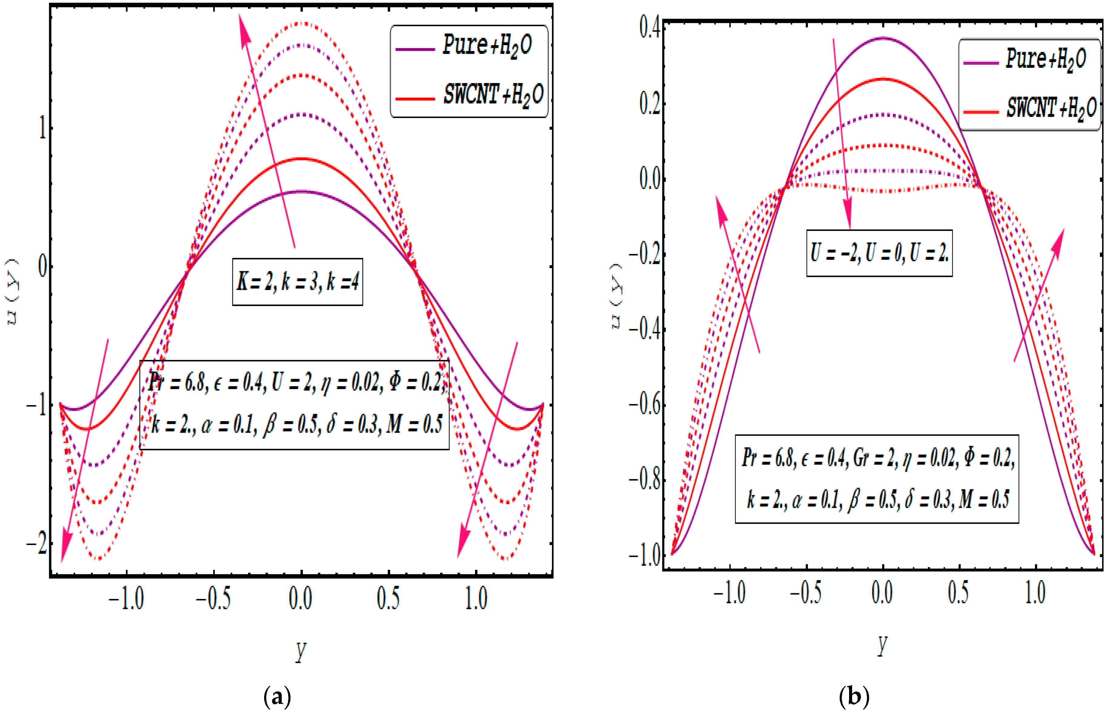
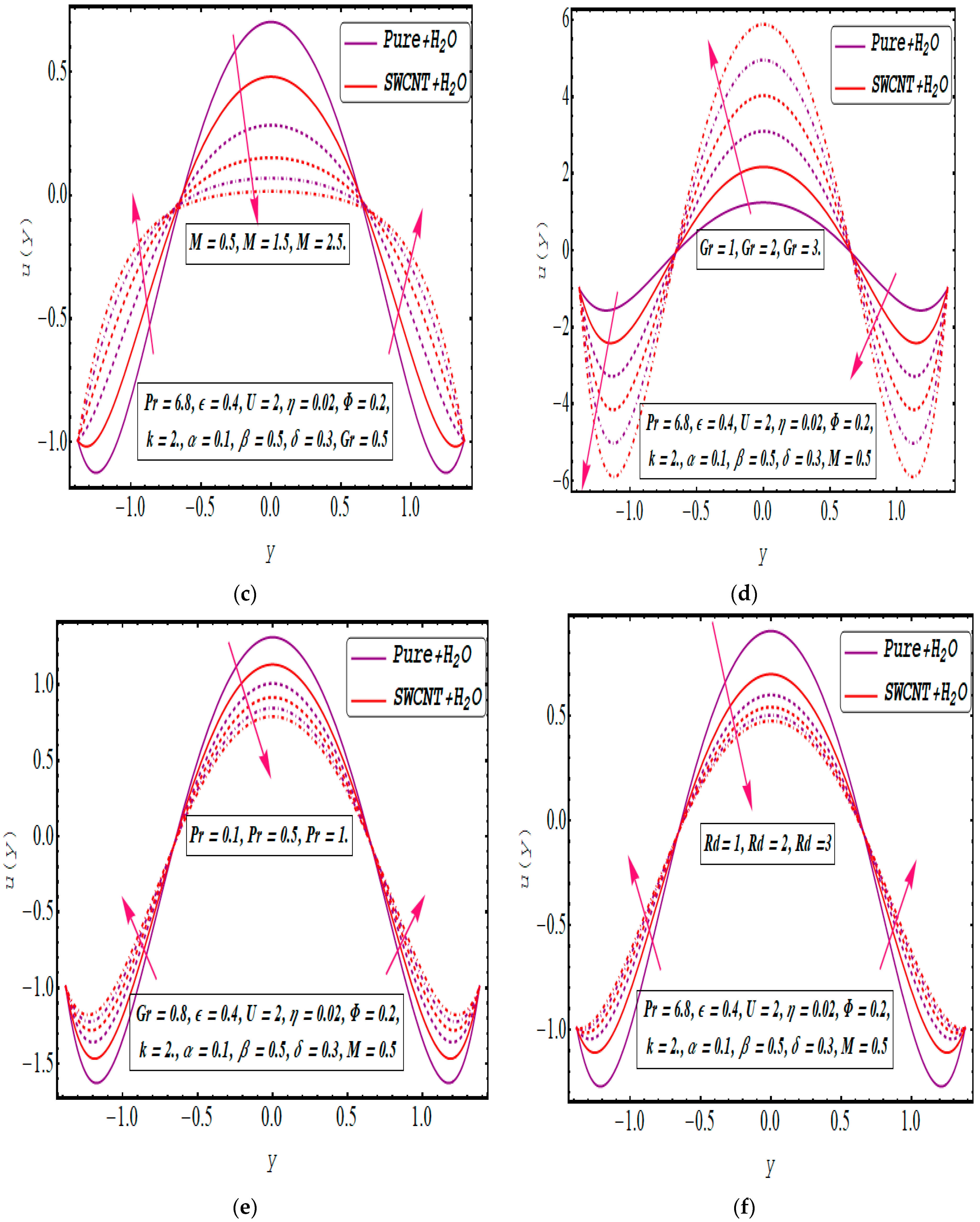
Figure 2a–e illustrate the variations in the velocity profile due to changes in different parameters. The velocity of an ionic aqueous solution exceeds that of the SWCNT–water ionic nanofluid. This result is consistent with the higher thermal conductivity of carbon nanotubes, which facilitates faster heat dissipation compared to pure water. In the SWCNT–water nanofluid, the reduced kinetic energy of fluid particles leads to a decrease in the velocity profile. Table 1 enumerates the thermophysical properties of specific parameters for SWCNTs and water, including specific heat capacity, density, thermal conductivity, and thermal expansion coefficient. Assuming a relative permittivity of 80 for water and an electric field strength of up to 1 kV/m, the Helmholtz–Smoluchowski velocity is approximately 2 m/s. The Debye length parameter (k) spans from O(1) to O(100) with bulk ionic concentrations ranging from 1 μM to 1 mM. The impact of varying the nanoparticle volume percentage from 0.1 to 0.3 vol% is depicted, with the particle number fixed at 0.2 vol%. The Prandtl number for water ranges from 1.7 to 13.7.
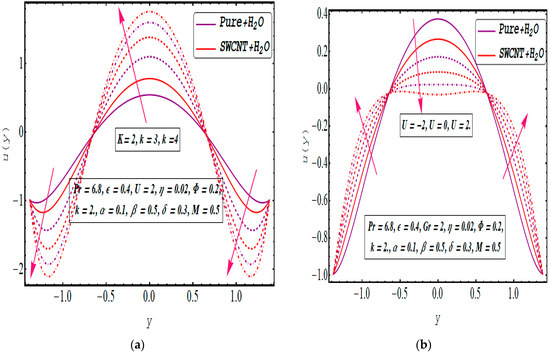
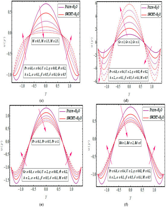
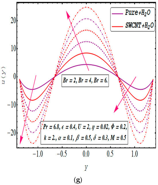
Figure 2.
(a–g) illustrate the velocity profiles u(y) for different values of the k, , Gr, U, Rd, Pr, and Br.

Table 1.
Thermophysical properties of pure water and single-walled carbon nanotubes (see ref. [51]).
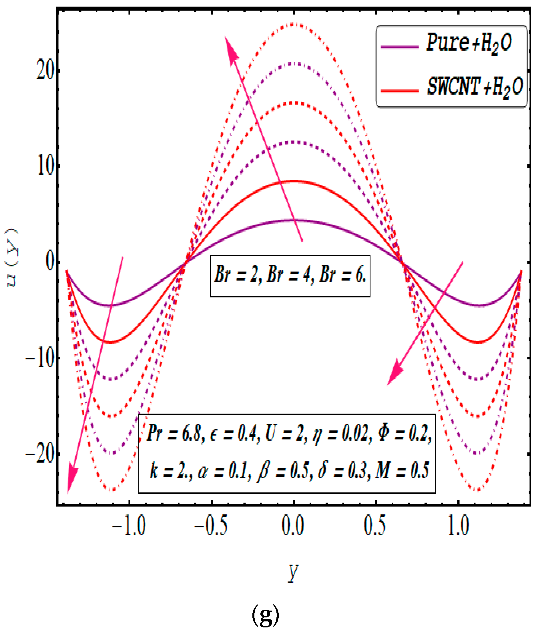
In Figure 2a, an increase in the Debye length parameter (k) results in an increased velocity. Physically, a higher (k) typically reduces the thickness of the electric double layer (EDL), enhancing electroosmotic forces that drive the electroosmotic velocity in the direction of peristaltic pumping. The fluid acceleration is a direct consequence of the elevated Debye length parameter. The diagram shows that velocity reaches its maximum for a negative value of (U) and minimum for a positive value of (U). This behavior is explained by U = −1 representing a supportive electric field (i.e., the electric field in the direction of peristaltic pumping), U = 0 indicating no electric field, and U = 1 corresponding to opposing electric body forces. Figure 2b depicts the velocity profile’s response to different values of the Helmholtz–Smoluchowski (HS) velocity parameter, which represents the velocity generated by the acceleration of ionic species due to electroosmotic forces. Figure 2c shows that an increase in the Hartmann number (M) leads to a decrease in the velocity field. A higher Hartmann number generates strong opposing Lorentz forces that resist the acceleration of fluid particles, reducing their velocity. In Figure 2d, an increase in the Grashof number (Gr), indicative of buoyancy forces dominating over viscous forces, enhances the velocity profile. A higher Grashof number is associated with a temperature difference within the fluid, quantifying the prevalence of buoyancy forces over viscous forces. Figure 2e illustrates that an increase in the Prandtl number (Pr) leads to a decrease in velocity. Figure 2f shows the impact of the radiation parameter on axial velocity, where a higher Reynolds number corresponds to a reduction in velocity. Finally, Figure 2g illustrates that an increase in the Brinkman number results in an augmented velocity field.
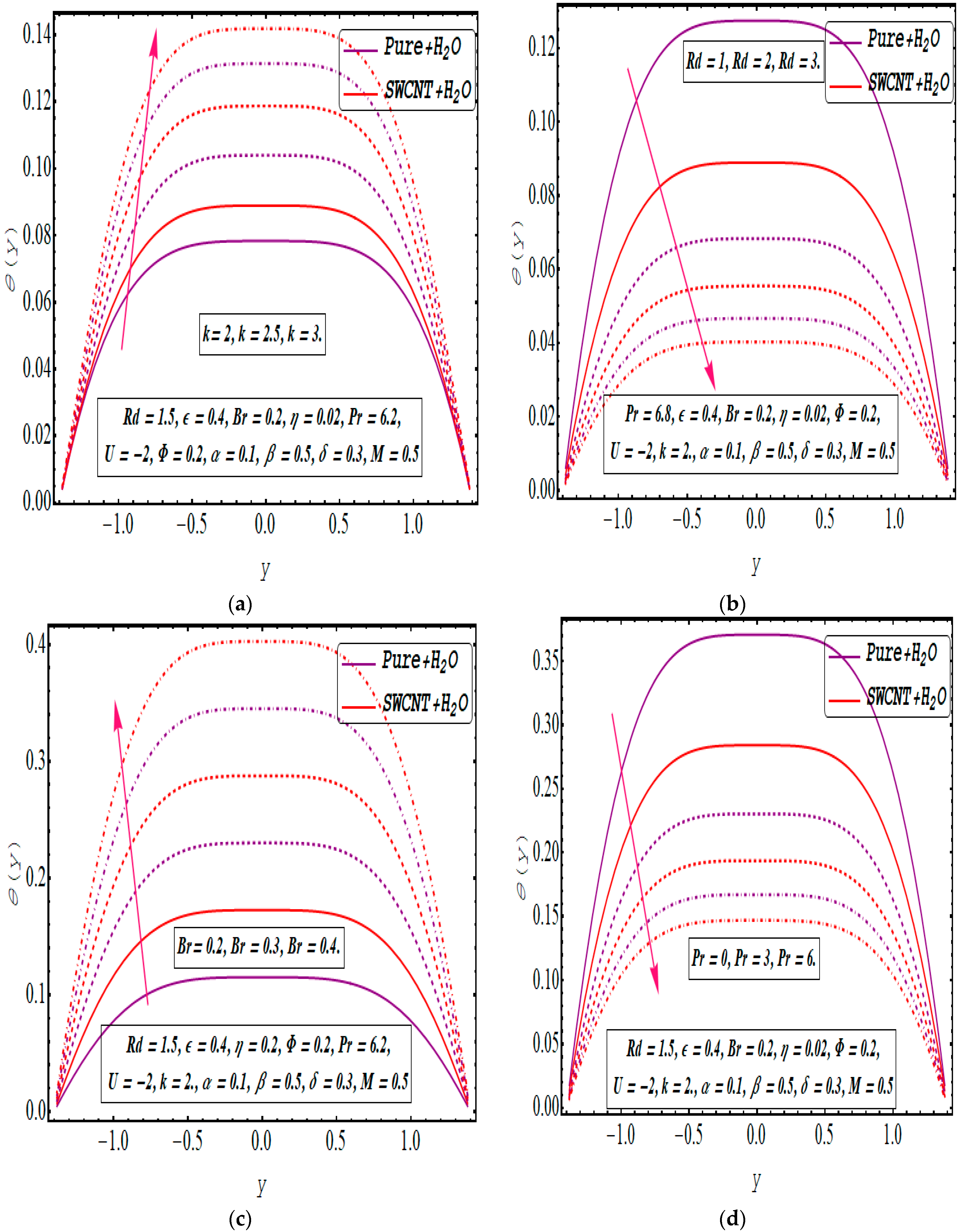
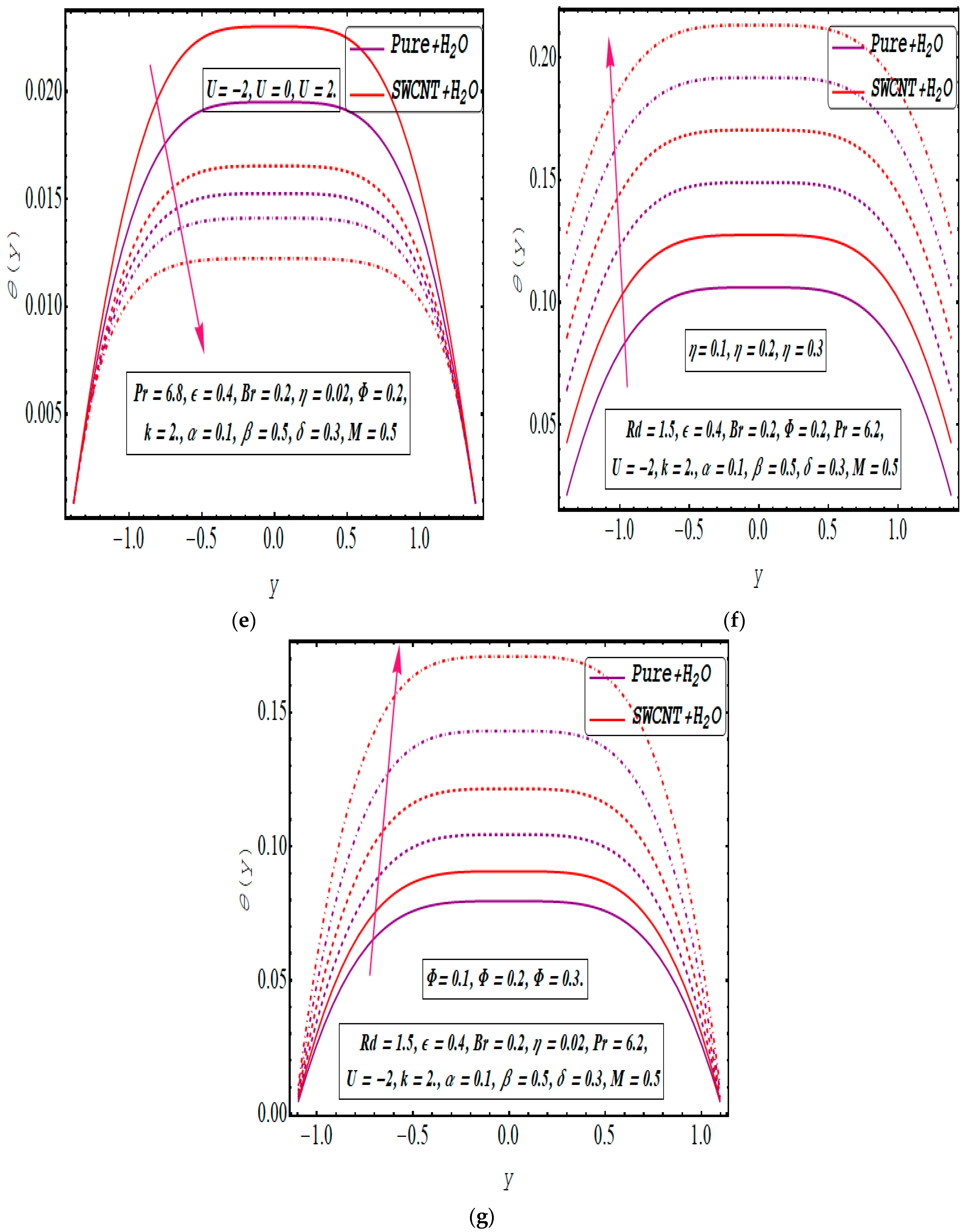
Figure 3a–g illustrate the influence of various embedded parameters on the temperature distribution. In Figure 3a, an increase in the Debye length parameter (k) correlates with a temperature rise. The graph shows a consistent temperature increase with the elevation of (k), which aligns with the physical rationale that a higher (k) enhances the kinetic energy of fluid particles, resulting in elevated temperatures. The presence of SWCNTs lowers the temperature of the water ionic solution, due to the rapid heat dissipation facilitated by the enhanced thermal conductivity of the nanotubes. This property makes carbon nanotube suspensions effective coolants in industrial applications. Figure 3b demonstrates a declining temperature distribution in relation to the radiation parameter. In Figure 3c, the temperature distribution rises with an increase in the Brinkman number, reflecting augmented heat generation due to viscous dissipation through shear stress. Consequently, higher (Br) values result in elevated temperatures. In Figure 3d, an increase in the Prandtl number reduces the temperature profile. Figure 3e shows that the temperature decreases for positive values of the Helmholtz–Smoluchowski (HS) velocity parameter but increases for negative values. This behavior is attributed to accelerated fluid particles generating more heat in the presence of an assisting electric field U = −1. Conversely, at U = 1, the electric field impedes fluid movement, reducing the kinetic energy of fluid particles and thereby decreasing the temperature. Figure 3f illustrates the fluctuation in fluid temperature for different values of the temperature slip parameter, showing an increase in temperature with a rising thermal slip parameter (η). Finally, Figure 3g depicts the impact of the volume fraction of single-walled carbon nanotubes (SWCNTs) on (θ). As the quantity of carbon nanotubes in the base fluid increases, there is a corresponding elevation in the temperature profile.
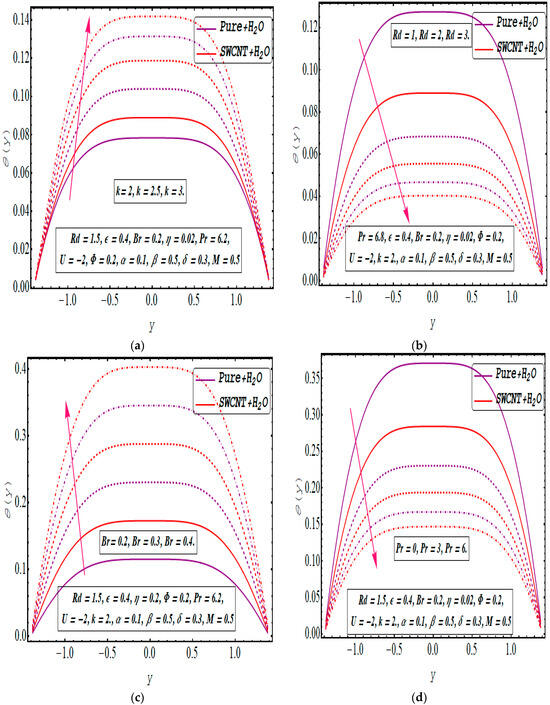
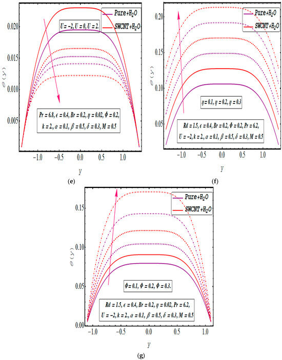
Figure 3.
(a–g): temperature profile θ(y) for different values of the k, Rd, U, Br, Pr, η, and .
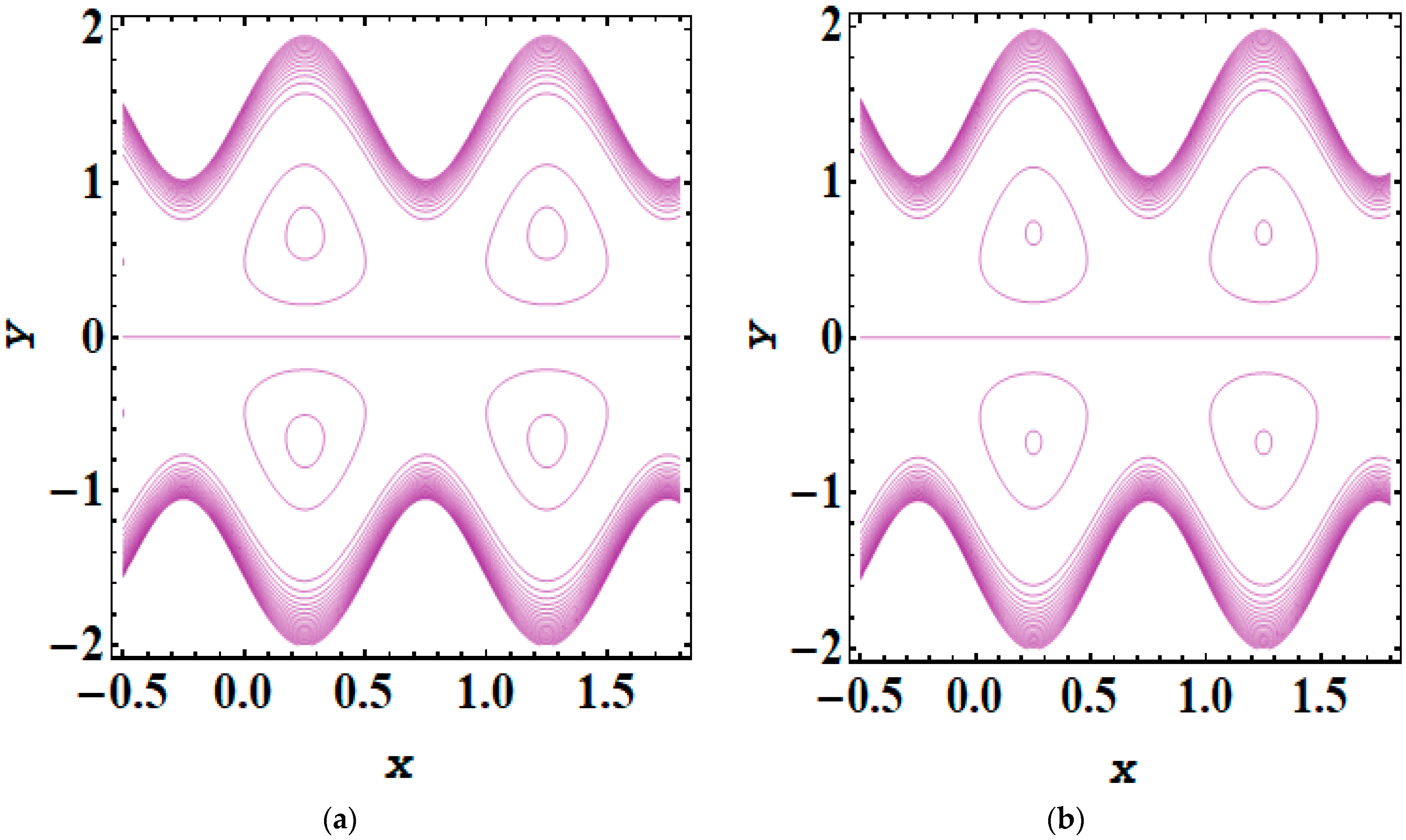
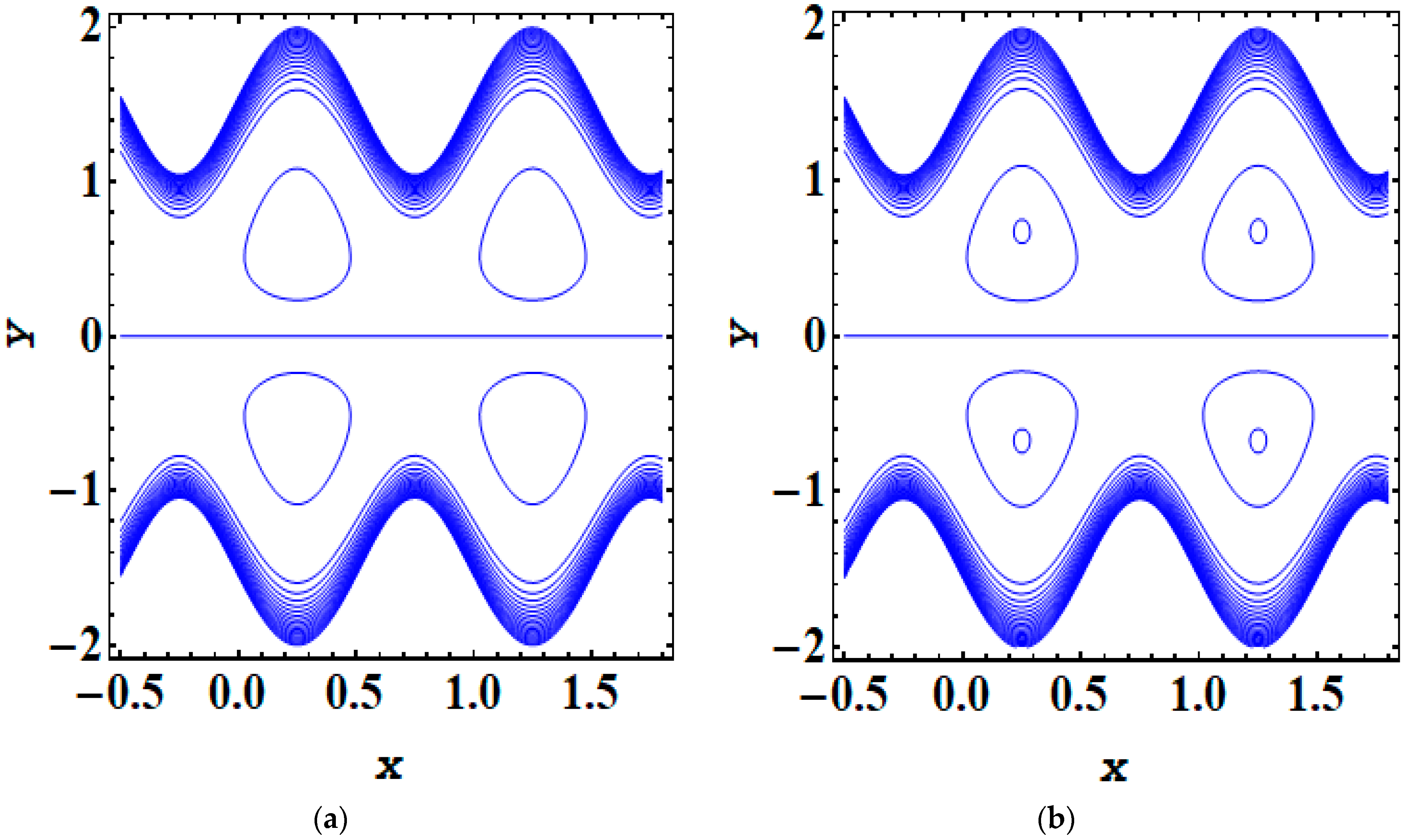
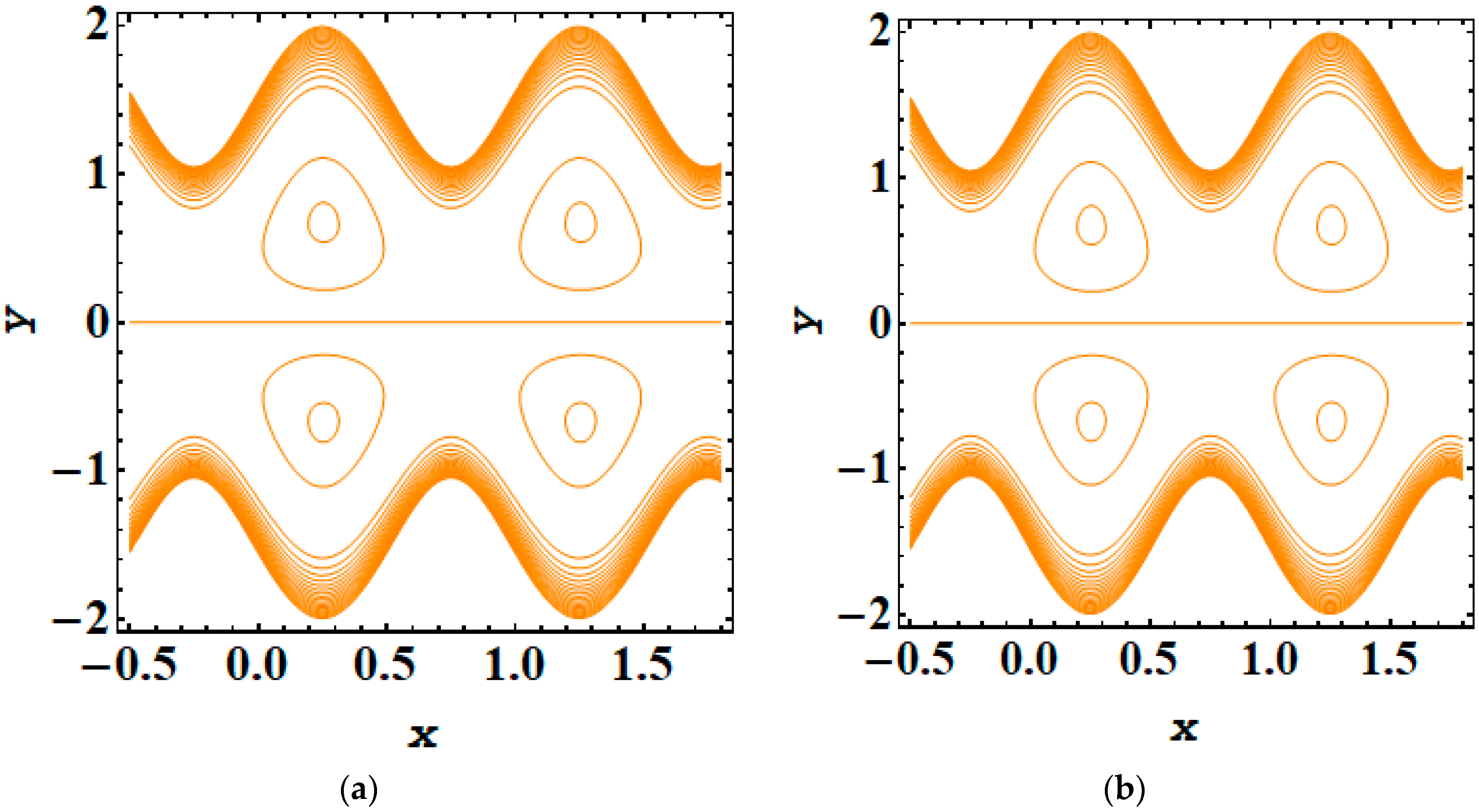
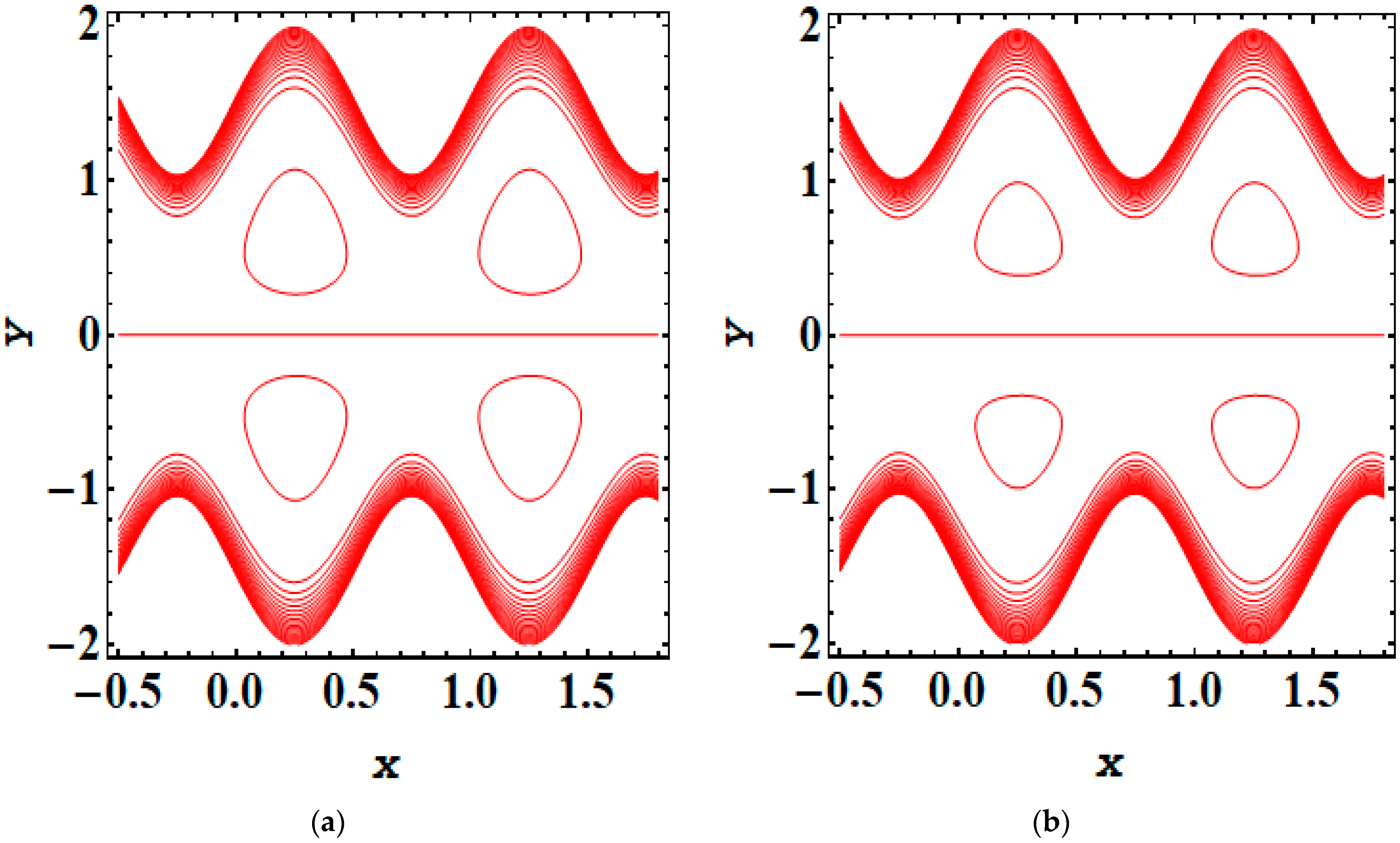
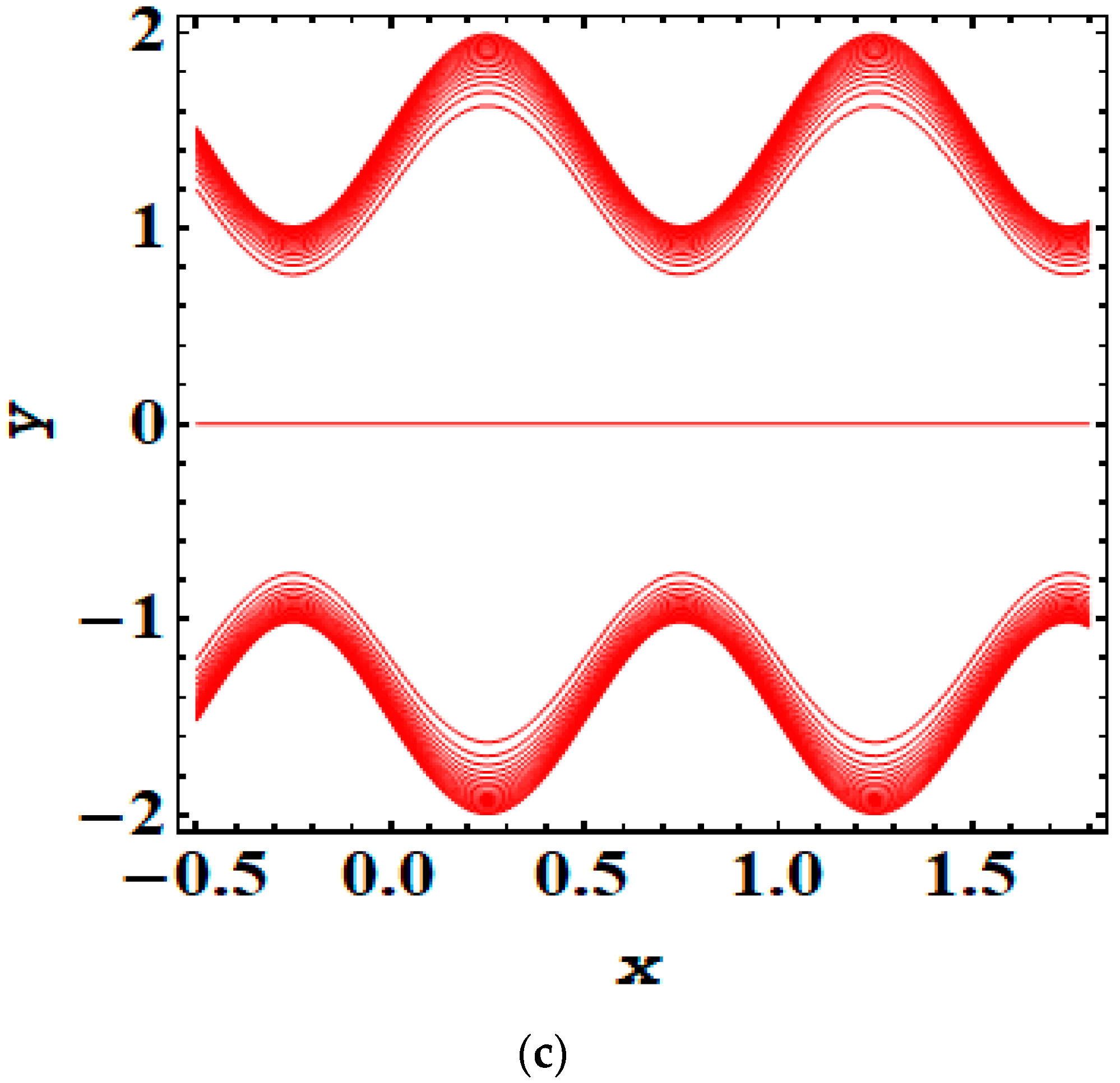
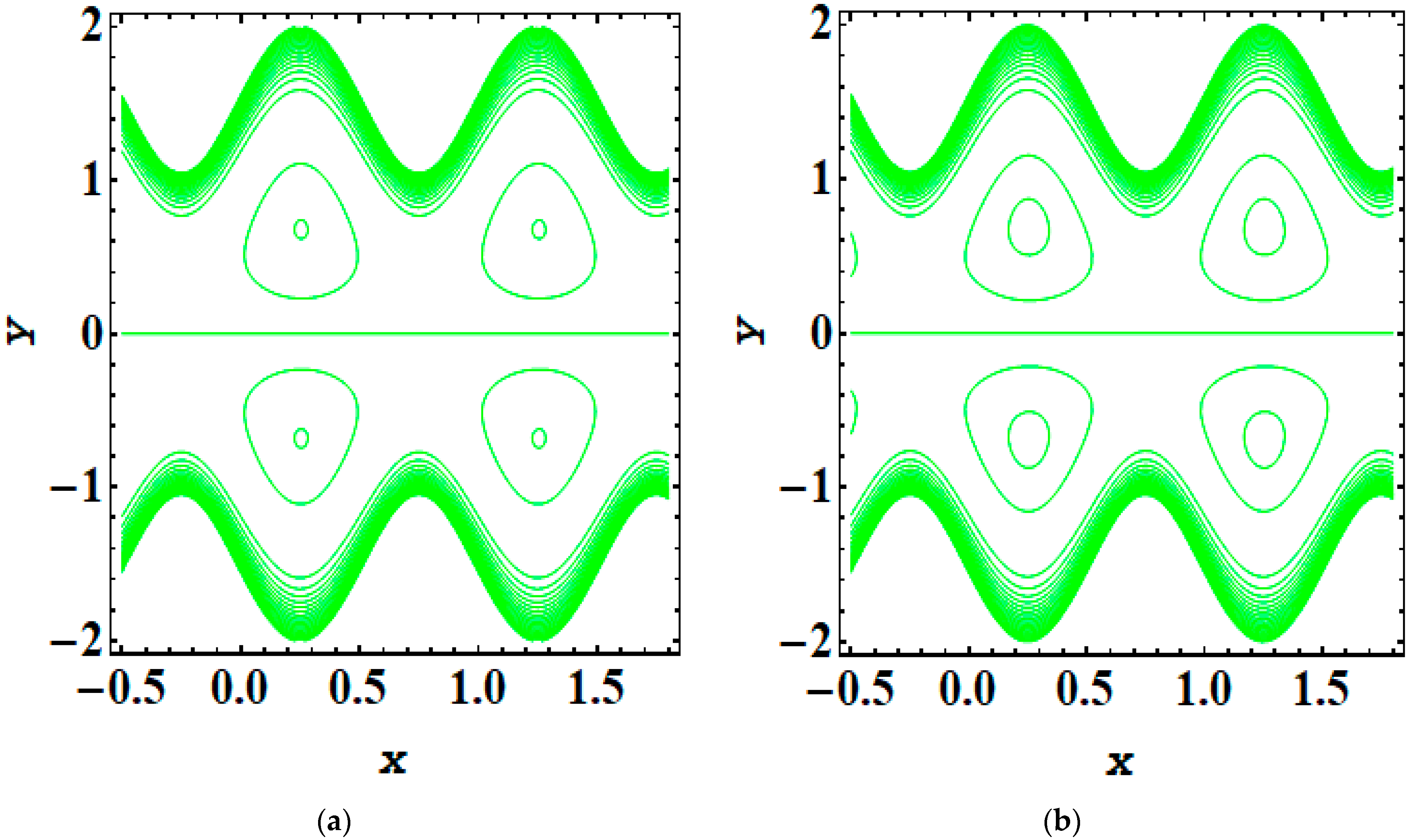
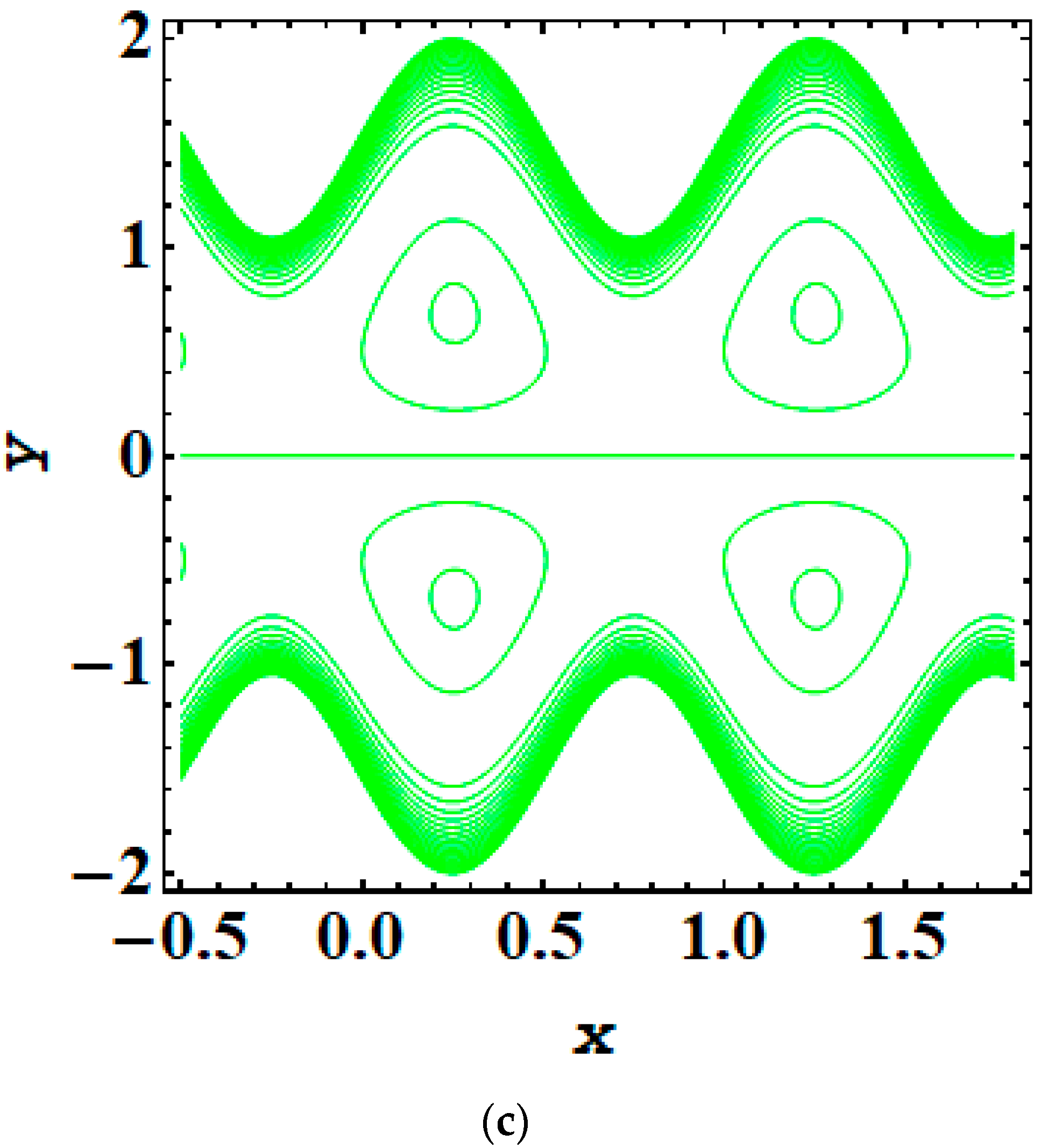
One of the most essential fluid dynamics flow features is streamlining. Examining the streamline patterns in light of the physical factors influencing the flow characteristics is crucial. It is essential for flow visualization. An essential characteristic of peristaltic flow pertains to the circulation of streamlines, known as trapping, and giving rise to a confined volume of fluid known as a bolus. Peristaltic waves effectively transmit this trapped bolus, significantly aiding fluid movement throughout the body. Figure 4, Figure 5, Figure 6, Figure 7, Figure 8, Figure 9 and Figure 10 are constructed to investigate the occurrence of trapping under various conditions for SWCNTs + water nanofluid. The Debye length parameter (k) represents the characteristic length scale over which charged particles in the fluid interact. Its impact on trapping is evident in Figure 4a–c, where an increase in k leads to the enlargement of the trapping bolus due to the mobilization of ionic species within the fluid medium. This is due to the extended influence of electrostatic forces, affecting the distribution and movement of charged particles. The Brinkman number (Br) characterizes the ratio of viscous to inertial forces in a porous medium. A higher Brinkman number in Figure 5a–c signifies dominance of viscous forces, which tend to resist the formation of trapping boluses. Consequently, an increase in this number leads to a reduction in the size of the trapping bolus due to enhanced viscous dissipation. The Prandtl number (Pr) relates the momentum diffusivity to the thermal diffusivity of a fluid. As the Prandtl number increases (Figure 6a–c), the thermal boundary layer becomes thicker than the momentum boundary layer. This results in more trapping boluses being formed since heat transfer mechanisms influence fluid motion, affecting the circulation of streamlines. When an electric field is applied in the direction of peristaltic propulsion (Figure 7a–c), it significantly influences the behavior of charged particles within the fluid. This leads to additional streamlines and trapped boluses as the electric field interacts with the fluid medium, altering its flow pattern. The Grashof number (Gr) signifies the ratio of buoyancy to viscous forces in a fluid flow. An increase in the Grashof number Figure 8a–c indicates dominance of buoyancy forces, which promote the formation of additional streamlines and trapped boluses. This occurs because higher Grashof numbers lead to more vigorous fluid motion, enhancing the trapping phenomenon. The Hartmann number characterizes the ratio of electromagnetic and viscous forces in a conductive fluid subjected to a magnetic field. In Figure 9a–c, a higher Hartmann number results in a decrease in the size of the trapping bolus. This is attributed to Lorentz forces exerted on the fluid flow, which exert control over its velocity, causing retardation and thus reducing the extent of trapping. The radiation parameter reflects the importance of thermal radiation in a fluid flow. As depicted in Figure 10a–c, an increase in the radiation parameter leads to a larger trapped bolus. This is because higher radiation parameters imply a more significant influence of radiative heat transfer on fluid dynamics, altering temperature distributions and consequently affecting the formation and size of trapping boluses.
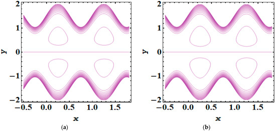

Figure 4.
Streamlines for SWCNT+H2O for (a) k = 2, (b) k = 2.2, and (c) k = 2.4.
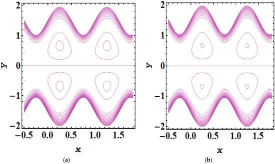
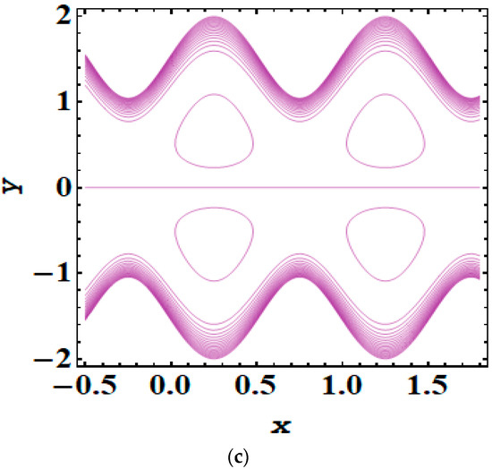
Figure 5.
Streamlines for SWCNT+H2O for (a) Br = 2, (b) Br = 4, and (c) Br = 6.
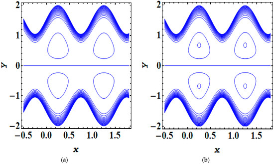
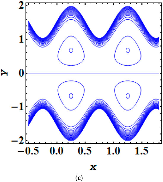
Figure 6.
Streamlines for SWCNT+H2O for (a) Pr = 1, (b) Pr = 2, and (c) Pr = 3.

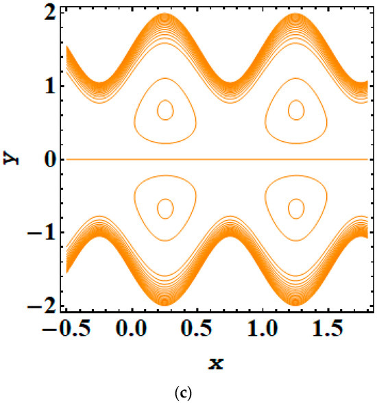
Figure 7.
Streamlines for SWCNT+H2O for (a) U = −2, (b) U = 0, and (c) U = 2.
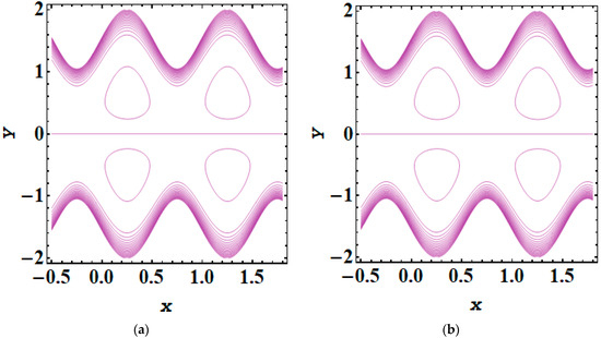
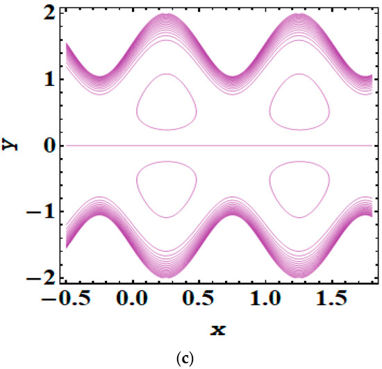
Figure 8.
Streamlines for SWCNT+H2O for (a) Gr = 6, (b) Gr = 7, and (c) Gr = 8.
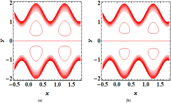

Figure 9.
Streamlines for SWCNT+H2O for (a) M = 0.2, (b) M = 0.7, and (c) M = 1.2.
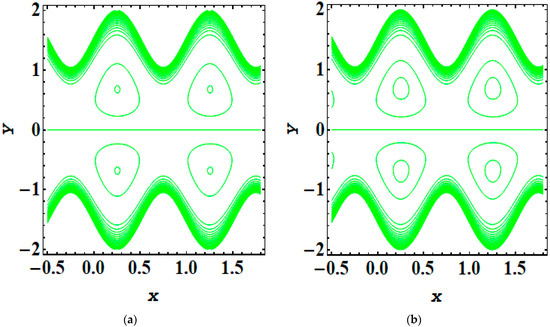
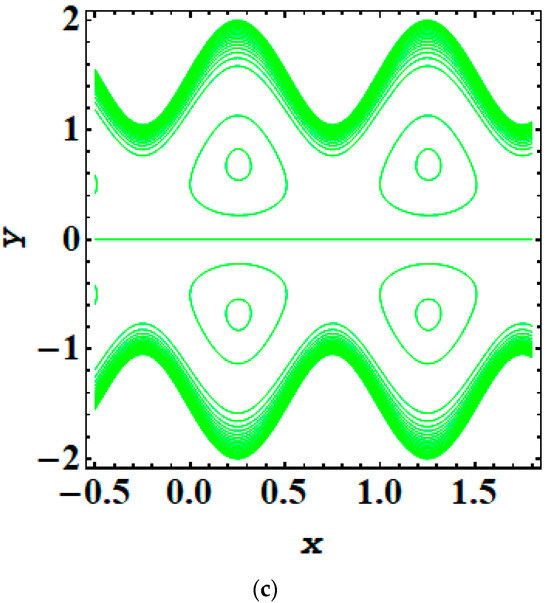
Figure 10.
Streamlines for SWCNT+H2O for (a) Rd = 1, (b) Rd = 2, and (c) Rd = 2.
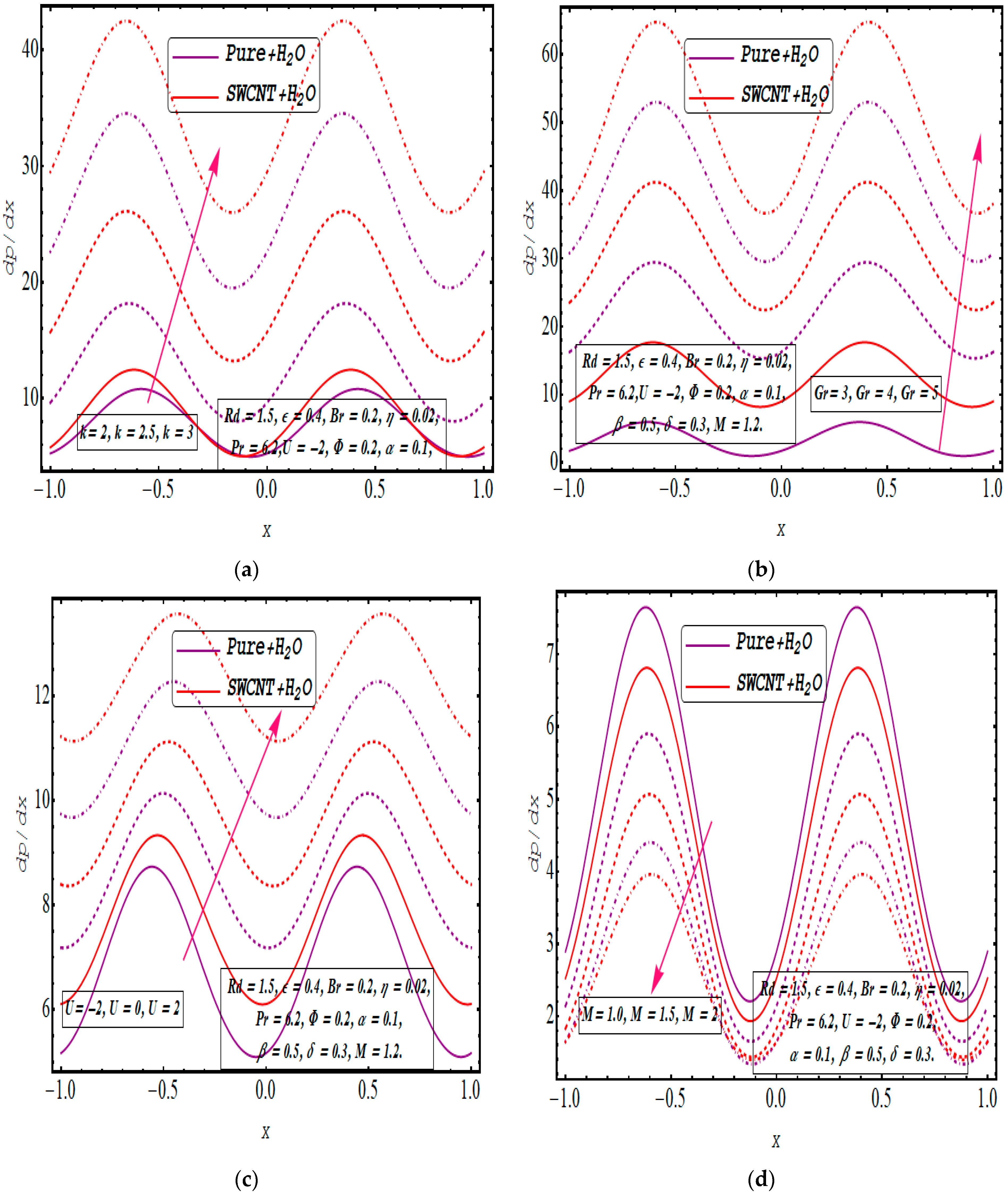
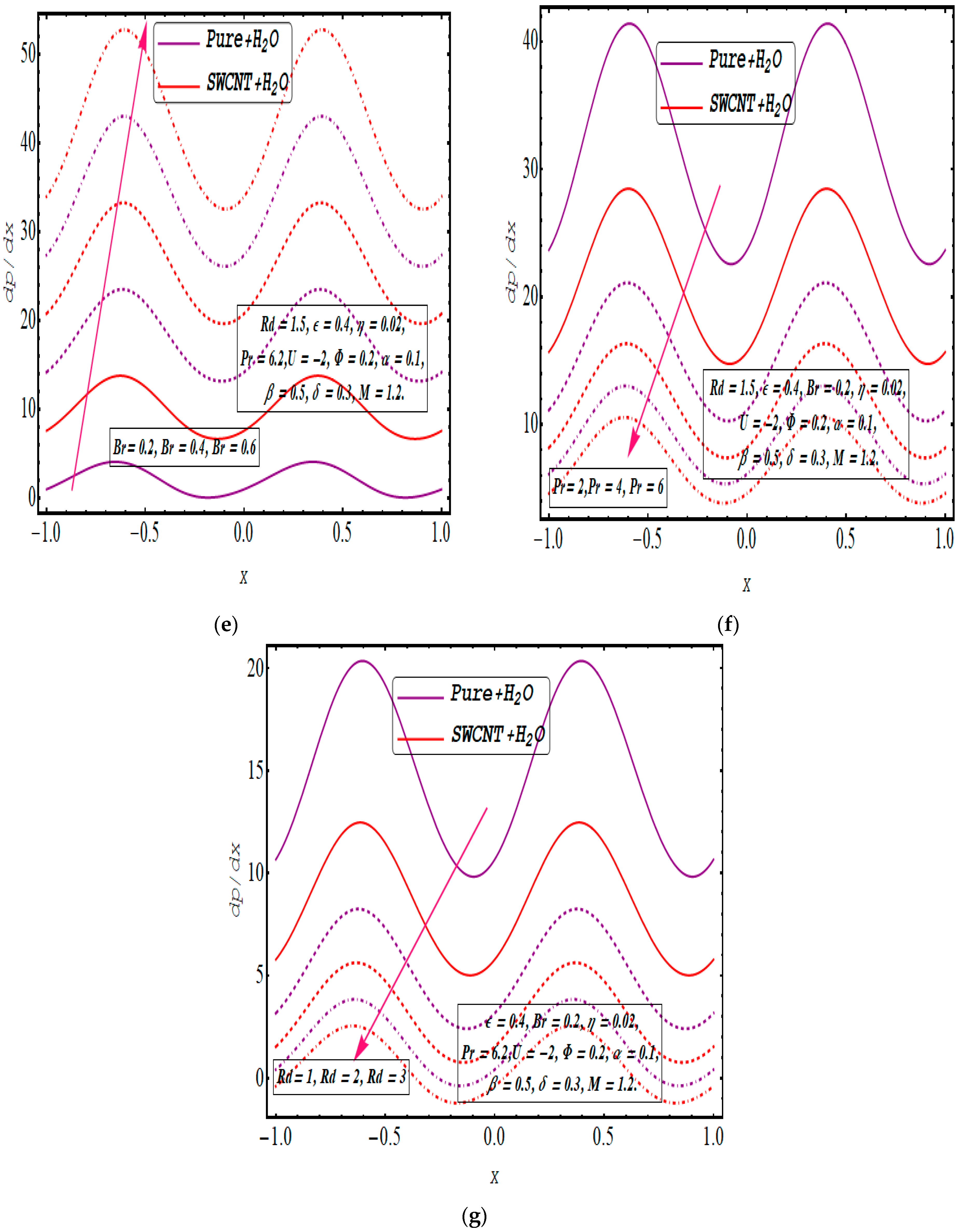
Figure 11a–g illustrate the response of the pressure gradient to developments in various pertinent parameters. The influence of the Debye length parameter (k) on the pressure gradient is presented in Figure 11a, where an increase in k corresponds to an elevation in the pressure gradient. A larger Debye length implies stronger electrostatic screening, allowing more ionic species to mobilize within the fluid. This increased mobility enhances the momentum transfer within the fluid, resulting in a higher pressure gradient. The electrostatic interactions between charged particles influence the fluid’s ability to transmit momentum, thereby affecting the pressure gradient. Similarly, Figure 11b shows that the pressure gradient increases with a rise in the Grashof number. The Grashof number reflects the ratio of buoyancy to viscous forces. As the Grashof number increases, buoyancy-driven flow becomes more dominant, leading to stronger fluid motion and, thus, a higher pressure gradient. This increase in pressure gradient is attributed to the enhanced convective heat transfer and fluid mixing associated with higher Grashof numbers. In Figure 11c, it is evident that the electric field’s facilitation of peristaltic transport results in an advancement of the pressure gradient. However, the assisting pressure gradient tends to decrease in the absence of an electric field or under an opposing electric field. In the former, where peristaltic pumping is the sole source of pressure gradient generation, the net assisting pressure gradient is lower. In the latter, the negative electroosmotic velocity creates a retarding pressure gradient opposing peristaltic pumping, further reducing the net assisting pressure gradient. Figure 11d explores pressure gradient variation with an increased Hartmann number (M), revealing that the pressure gradient diminishes as M magnifies. The Hartmann number represents the ratio of electromagnetic forces to viscous forces. A higher Hartmann number indicates stronger electromagnetic forces, which can suppress fluid motion and momentum transfer, thereby reducing the pressure gradient. Examining the Brinkman number (Br) in Figure 11e, it is apparent that an increase in Br corresponds to a rise in the pressure gradient. The Brinkman number characterizes viscous to inertial forces ratio in a porous medium. A higher Brinkman number implies a dominance of viscous forces, which resist fluid motion. Consequently, an increase in the Brinkman number leads to enhanced viscous dissipation, resulting in a higher pressure gradient. The impact of the Prandtl number (Pr) on the pressure gradient is demonstrated in Figure 11f, showing a decrease in the pressure gradient as the Prandtl number increases. The Prandtl number relates the momentum diffusivity to the thermal diffusivity of a fluid. As the Prandtl number increases, the thermal boundary layer becomes thicker than the momentum boundary layer. This decreases the pressure gradient since the fluid’s ability to transmit momentum is reduced due to the increased dominance of thermal effects. Finally, in Figure 11g, the influence of the radiation parameter (Rd) on the pressure gradient is depicted, indicating a drop in the pressure gradient with an increase in Rd. The radiation parameter reflects the importance of thermal radiation in a fluid flow. An increase in the radiation parameter implies a significant influence of radiated heat transfer, which can lead to temperature gradients that hinder fluid motion. Consequently, the pressure gradient decreases as the radiation parameter increases due to the reduced momentum transfer within the fluid.
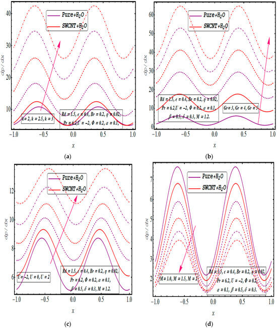
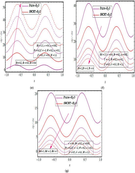
Figure 11.
(a–g): pressure gradient for variation in k, Gr, U, M, Pr, Br, and Rd.
Table 2 and Table 3 compare velocity and temperature between the study conducted by Akram et al. [44] and the limiting case of the current problem. The tables show a clear, close agreement between the solutions.
Table 2.
Comparison of the velocity profile from the current investigation with the results obtained by Akram et al. [44].
Table 3.
Comparison of the temperature profile from the current investigation with the results obtained by Akram et al. [46].
6. Conclusions
A theoretical investigation is underway in this model to examine the electroosmotically controlled peristaltic pumping of SWCNTs + water ionic nanofluids through ciliated channels. Cilia influence fluid flow in biological systems and microfluidic devices by enhancing propulsive mechanisms and sensing functions. The analysis also considers the impact of heat dissipation due to viscous forces when assessing fluid flow in the presence of buoyant forces. Ciliated boundary conditions for temperature and velocity are applied along the channel walls. The regular perturbation technique helps simplify the nonlinear and coupled set of equations, yielding an approximate solution to the problem. The noteworthy outcomes of the current analysis, as elucidated in the discussion, include the following:
- The velocity tends to increase as the Debye length parameter increases.
- The temperature rises when the electric field is added and decreases when opposed.
- As the magnitude of the Debye length parameter rises, the trapping bolus also increases.
- Adding and removing the electric field significantly impacts trapping phenomena.
- The incorporation of SWCNTs tends to reduce the temperature profile, primarily due to the heightened thermal conductivity of the base fluid.
- The pumping and flow characteristics increase when an electric field is added and decrease when it is opposed.
- The addition or opposition of an electric field greatly influences the dynamics of trapping phenomena.
- The outcomes of this model find potential applications in biomicrofluidics, particularly in the development of controlled medication delivery systems aimed at identifying and targeting cancerous cells during treatment. Additionally, this model holds promise for enhancing the efficiency of solar heat collectors and various cooling systems.
Author Contributions
Conceptualization, R.E.; Methodology, R.E.; Validation, J.M.; Formal analysis, S.M.S.; Investigation, J.M.; Writing—original draft, J.M.; Writing—review & editing, S.M.S. All authors have read and agreed to the published version of the manuscript.
Funding
This research received no external funding.
Data Availability Statement
Data are contained within the article.
Conflicts of Interest
The authors declare no conflicts of interest.
Appendix A
References
- Reuss, F. Sur un nouvel effect de l electricite glvanique. Mem. Soc. Imp. Nat. Mosc. 1890, 2, 326–339. [Google Scholar]
- Kirby, B.J. Chapter 6: Electroosmosis. In Micro Nanoscale Fluid Mechanics: Transport in Microfluidic Devices; Cambridge University Press: Cambridge, UK, 2010. [Google Scholar]
- Bruus, H. Theoretical Microfluidics; Oxford University Press: New York, NY, USA, 2017. [Google Scholar]
- Arangoa, M.A.; Campanero, M.A.; Popineau, Y.; Irache, J.M. Electrophoretic separation and characterization gliadin fractions from isolates and nanoparticulate drug delivery systems. Chromstograhia 1999, 50, 243–246. [Google Scholar] [CrossRef]
- Chang, H.; Chen, H.; Hsieh, M.M.; Tseng, W.L. Electrophoretic separation of DNA in the presence of electrooosmotic flow. Rev. Anal. Chem. 2000, 19, 45–74. [Google Scholar] [CrossRef]
- Fung, Y.C.; Yih, C.S. Peristaltic transport. J. Appl. Mech. 1968, 35, 669–675. [Google Scholar] [CrossRef]
- Srivastava, L.M.; Srivastava, V.P.; Sinha, S.N. Peristaltic transport of a physiological fluid. Biorheology 1983, 20, 153–166. [Google Scholar] [CrossRef] [PubMed]
- Saleem, A.; Qaiser, A.; Nadeem, S.; Ghalambaz, M.; Issakhov, A. Physiological Flow of Non-Newtonian Fluid with Variable Density inside a Ciliated Symmetric Channel Having Compliant Wall. Arab. J. Sci. Eng. 2020, 46, 801–812. [Google Scholar] [CrossRef]
- Chakraborty, S. Augmentation of peristaltic microflows through electro-osmotic mechanisms. J. Phys. D Appl. Phys. 2006, 39, 5356–5363. [Google Scholar] [CrossRef]
- Bandopadhyay, A.; Tripathi, D.; Chakraborty, S. Electroosmosis-modulated peristaltic transport in microfluidic channels. Phys. Fluids 2016, 28, 052002. [Google Scholar] [CrossRef]
- Ranjit, N.K.; Shit, G.C. Entropy generation on electro-osmotic flow pumping by a uniform peristaltic wave under magnetic environment. Energy 2017, 128, 649–660. [Google Scholar] [CrossRef]
- Akram, J.; Akbar, N.S.; Tripathi, D. Numerical study of the electroosmotic flow of Al2O3–CH3OH Sisko nanofluid through a tapered microchannel in a porous environment. Appl. Nanosci. 2020, 10, 4161–4176. [Google Scholar] [CrossRef]
- Ranjit, N.K.; Shit, G.C.; Sinha, A. Transportation of ionic liquids in a porous micro-channel induced by peristaltic wave with Joule heating and wall-slip conditions. Chem. Eng. Sci. 2017, 171, 545–557. [Google Scholar] [CrossRef]
- Bhatti, M.M.; Zeeshan, A.; Ellahi, R.; Ijaz, N. Heat and mass transfer of two-phase flow with Electric double-layer effects induced due to peristaltic propulsion in the presence of the transverse magnetic field. J. Mol. Liq. 2017, 230, 237–246. [Google Scholar] [CrossRef]
- Prakash, J.; Sharma, A.; Tripathi, D. Thermal radiation effects on electroosmosis modulated peristaltic transport of ionic nanoliquids in biomicrofluidics channel. J. Mol. Liq. 2018, 249, 843–855. [Google Scholar] [CrossRef]
- Tripathi, D.; Jhorar, R.; Bég, O.A.; Shaw, S. Electroosmosis modulated peristaltic biorheological flow through an asymmetric microchannel: A mathematical model. Meccanica 2018, 53, 2079–2090. [Google Scholar] [CrossRef]
- Prakash, J.; Ramesh, K.; Tripathi, D.; Kumar, R. Numerical simulation of heat transfer in blood flow altered by electroosmosis through tapered micro-vessels. Microvasc. Res. 2018, 118, 162–172. [Google Scholar] [CrossRef] [PubMed]
- Kattamreddy, V.R.; Makinde, O.D.; Reddy, M.G. Thermal analysis of MHD electro-osmotic peristaltic pumping of Casson fluid through a rotating asymmetric micro-channel. Indian J. Phys. 2018, 92, 1439–1448. [Google Scholar]
- Akram, J.; Akbar, N.S.; Tripathi, D. Blood-based graphene oxide nanofluid flow through capillary in the presence of electromagnetic fields: A Sutterby fluid model. Microvas. Res. 2020, 132, 104062. [Google Scholar] [CrossRef] [PubMed]
- Noreen, S.; Ain, Q. Entropy generation analysis on electroosmotic flow in non-Darcy porous medium via peristaltic pumping. J. Therm. Anal. Calorim. 2019, 137, 1991–2006. [Google Scholar] [CrossRef]
- Choi, S.; Eastman, J. Enhancing thermal conductivity of the fluids with nanoparticles. In Proceedings of the ASME International Mechanical Engineering Congress and Exposition, ASME, San Francisco, CA, USA, 12–17 November 1995. [Google Scholar]
- Tiwari, R.J.; Das, M.K. Heat transfer augmentation in a two-sided lid-driven differentially heated square cavity utilizing nanofluids. Int. J. Heat Mass Transf. 2007, 50, 2002–2018. [Google Scholar] [CrossRef]
- Sleigh, A. The Biology of Cilia and Flagella; MacMillian: New York, NY, USA, 1962; Volume 9, pp. 339–398. [Google Scholar]
- Christensen, S.T.; Pedersen, L.B.; Schneider, L.; Satir, P. Sensory cilia and integration of signal transduction in human health and disease. Traffic 2007, 8, 97. [Google Scholar] [CrossRef]
- Eggenschwiler, J.T.; Anderson, K.V. Cilia and developmental signaling. Annu. Rev. Cell Dev. Biol. 2007, 23, 345. [Google Scholar] [CrossRef] [PubMed]
- Ibanez-Tallon, I.; Heintz, N.; Omran, H. To beat or not to beat: Roles of cilia in development and disease. Hum. Mol. Genet. 2003, 12, R27–R35. [Google Scholar] [CrossRef] [PubMed]
- Davis, E.E.; Brueckner, M.; Katsanis, N. The emerging complexity of the vertebrate cilium: New functional roles for an ancient organelle. Dev. Cell 2006, 11, 9. [Google Scholar] [CrossRef] [PubMed]
- Maiti, S.; Pandey, S.K. Rheological fluid motion in tube by metachronal wave of cilia. arXiv 2013, arXiv:1308.3608v1. [Google Scholar] [CrossRef]
- Asha, S.K.; Namrata, K. Influence of metra chronal ciliary wave motion on peristalatic flow of nanofluid model of synovitis problem. AIP Adv. 2022, 12, 055217. [Google Scholar]
- Gholamalipour, P.; Siavashi, M.; Doranehgard, M.H. Eccentricity effects of heat source inside a porous annulus on the natural convection heat transfer and entropy generation of Cu-water nanofluid. Int. Commun. Heat Mass Transf. 2019, 109, 104367. [Google Scholar] [CrossRef]
- Turkyilmazoglu, M. An analytical treatment for the exact solutions of MHD flow and heat over two–three dimensional deforming bodies. Int. J. Heat Mass Transf. 2015, 90, 781–789. [Google Scholar] [CrossRef]
- Turkyilmazoglu, M. Corrections to long wavelength pproximation of peristalsis viscous fluid flow within a wavy channel. Chin. J. Phys. 2024, 89, 340–354. [Google Scholar] [CrossRef]
- Zhang, L.; Bhatti, M.M.; Marin, M.; Mekheimer, K.S. Entropy analysis on the blood flow through anisotropically tapered arteries filled with magnetic zinc-oxide (ZnO) nanoparticles. Entropy 2020, 22, 1070. [Google Scholar] [CrossRef]
- Sharma, B.K.; Kumar, A.; Gandhi, R.; Bhatti, M.M.; Mishra, N.K. Entropy Generation and Thermal Radiation Analysis of EMHD Jeffrey Nanofluid Flow: Applications in Solar Energy. Nanomaterials 2023, 13, 544. [Google Scholar] [CrossRef]
- Gandhi, R.; Sharma, B.K.; Mishra, N.K.; Al-Mdallal, Q.M. Computer Simulations of EMHD Casson Nanofluid Flow of Blood through an Irregular Stenotic Permeable Artery: Application of Koo-Kleinstreuer-Li Correlations. Nanomaterials 2023, 13, 652. [Google Scholar] [CrossRef] [PubMed]
- Waqas, H.; Khan, S.U.; Bhatti, M.M.; Imran, M. Significance of bioconvection in chemical reactive flow of magnetized Carreau–Yasuda nanofluid with thermal radiation and second-order slip. J. Therm. Anal. Calorim. 2020, 140, 1293–1306. [Google Scholar] [CrossRef]
- Zafar, S.; Khan, A.A.; Sait, S.M.; Ellahi, R. Numerical investigation on unsteady compressible flow of viscous fluid with convection under the effect of Joule heating. J. Comput. Appl. Mech. 2024, 55. [Google Scholar] [CrossRef]
- Kanwal, A.; Khan, A.A.; Sait, S.M.; Ellahi, R. Heat transfer analysis of magnetohydrodynamics peristaltic fluid with inhomogeneous solid particles and variable thermal conductivity through curved passageway. Int. J. Numer. Methods Heat Fluid Flow 2024, 34, 1884–1902. [Google Scholar] [CrossRef]
- Khan, A.A.; Fatima, G.; Sait, S.M.; Ellahi, R. Electromagnetic effects on two-layer peristalsis flow of Powell–Eyring nanofluid in axisymmetric channel. J. Therm. Anal. Calorim. 2024, 149, 3631–3644. [Google Scholar] [CrossRef]
- Ellahi, R. The effects of MHD and temperature dependent viscosity on the flow of non-Newtonian nanofluid in a pipe: Analytical solutions. Appl. Math. Model. 2013, 37, 1451–1457. [Google Scholar] [CrossRef]
- Ellahi, R.; Zeeshan, A.; Hussain, F.; Asadollahi, A. Peristaltic blood flow of couple stress fluid suspended with nanoparticles under the influence of chemical reaction and activation energy. Symmetry 2019, 11, 276. [Google Scholar] [CrossRef]
- Choi, S.U.S.; Zhang, Z.G.; Yu, W.; Lockwood, F.E.; Grulke, E.A. Anomalous thermal conductivity enhancement in nanotube suspensions. Appl. Phys. Lett. 2007, 79, 2252–2254. [Google Scholar] [CrossRef]
- Kam, N.W.S.; O’Connell, M.; Wisdom, J.A.; Dai, H. Carbon nanotubes as multifunctional biological transporters and near-infrared agents for selective cancer cell destruction. Proc. Natl. Acad. Sci. USA 2017, 102, 11600–11605. [Google Scholar] [CrossRef]
- Akram, J.; Akbar, N.S.; Tripathi, D. Electoosmosis augmented MHD peristaltic transport of SWCNTs suspention in aqueous media. J. Therm. Anal. Calorim. 2021, 147, 2509–2526. [Google Scholar] [CrossRef]
- Lardner, T.J.; Shack, W.J. Cilia transport. Bull. Math. Biol. 1972, 34, 325–335. [Google Scholar] [CrossRef] [PubMed]
- Akbar, N.S.; Tripathi, D.; Khan, Z.H.; Beg, O.A. Mathematical model for ciliary-induced transport in MHD flow of Cu-H2O nanofluid with magnetic induction. Chin. J. Phys. 2017, 55, 947–962. [Google Scholar] [CrossRef]
- Tripathi, D.; Sharma, A.; Bég, O.A. Electrothermal transport of nanofluids via peristaltic pumping in a finite micro-channel: Effects of Joule heating and Helmholtz-Smoluchowski velocity. Int. J. Heat Mass Trans. 2017, 111, 138–149. [Google Scholar] [CrossRef]
- Narla, V.K.; Tripathi, D.; Bég, O.A. Electro-osmotic nanofluid flow in a curved microchannel. Chin. J. Phys. 2020, 67, 544–558. [Google Scholar] [CrossRef]
- Tripathi, D.; Yadav, A.; Bég, O.A. Electro-kinetically driven peristaltic transport of viscoelastic physiological fluids through a finite length capillary. Math. Model. Math. Biosci. 2017, 283, 155–168. [Google Scholar] [CrossRef]
- Prakash, J.; Tripathi, D. Electroosmotic flow of Williamson ionic nanoliquids in a tapered microfluidic channel in presence of thermal radiation and peristalsis. J. Mol. Liq. 2018, 256, 352–371. [Google Scholar] [CrossRef]
- Ellahi, R.; Sait, S.M.; Shehzad, N.; Mobin, N. Numerical simulation and mathematical modeling of electroosmotic Couette-Poiseuille flow of MHD power-law nanofluid with entropy generation. Symmetry 2019, 11, 1038. [Google Scholar] [CrossRef]


Disclaimer/Publisher’s Note: The statements, opinions and data contained in all publications are solely those of the individual author(s) and contributor(s) and not of MDPI and/or the editor(s). MDPI and/or the editor(s) disclaim responsibility for any injury to people or property resulting from any ideas, methods, instructions or products referred to in the content. |
© 2024 by the authors. Licensee MDPI, Basel, Switzerland. This article is an open access article distributed under the terms and conditions of the Creative Commons Attribution (CC BY) license (https://creativecommons.org/licenses/by/4.0/).