A Mathematical Analysis and Simulation of the F-L Effect in Two-Layered Blood Flow through the Capillaries Remote from the Heart and Proximate to Human Tissue

Abstract

In this paper, we have provided a mathematical analysis of an empirical result, namely, the Fahraeus–Lindqvist effect, a phenomenon that occurs in capillary tubes with a diameter lower than 0.3 mm. According to this effect, in capillary tubes under 0.3 mm in diameter, the apparent viscosity of blood decreases as the diameter of the tube decreases, making flow possible in these vessels. A two-phase blood flow mathematical model for human capillaries has been presented here. According to Haynes’ theory, blood is separated into two layers when it flows from the capillary. It is assumed that the first layer is plasma, and the second layer is the core layer. The plasma layer flows near the wall of the capillary, and the core layer flows along the axis of the capillary. Further, the core layer is assumed to be a mixture of two phases: one is the plasma, and the other is that of RBCs. For mathematical modeling purposes, a curvilinear coordinate system has been adopted, with physical quantities used in tensorial form. Derived equations are solved to find the effective viscosity, which depends upon the radius of the capillary; that is, it reduces viscosity to make blood flow possible. A comparative study was conducted with the experimental result of this effect, and it was observed that the proposed two-phase blood flow model is much closer to the experimental data than the single-phase blood flow model, and both have the same trends. After validation of the model with the experimental result, this model was applied to human capillaries (diameter lower than 10 $\mathsf{\mu }\mathrm{m}$) to show the F-L effect, and the impact of various physiological quantities that are relevant to the flow of blood into human capillaries are also discussed here. The impact of hematocrit on various parameters has been demonstrated explicitly.

1. Introduction

Capillaries are the smallest vessel in the human body [1]. They are tiny branches of the arterioles. Their internal diameter is about 4 to 10 $\mathsf{\mu }\mathrm{m}$, less than 1/3 of a hair’s width [2,3]. They are composed of a single layer of flat cells. This layer not only forms the walls of the capillaries but also lines the other blood vessels and the heart, so all the blood in the body is contained within a single continuous envelope. Capillaries permeate every tissue of the body; indeed, no cell is more than a few thousandths of an inch from a capillary. The primary functions of the circulatory system take place in the capillary, i.e., the continuous unloading of cargo for the cells and the carrying away of the products of the cellular metabolism [3,4,5].

Capillaries are far away from the heart and narrow enough. Blood flow is already very low in arterioles due to the low heart pumping effect and high viscosity, so how is blood flow into capillaries possible? This happens due to the F-L effect [1]. It is a situation that happens in capillary-like tubes (diameter lower than 0.3 mm) [1]. The F-L effect was described independently by two Swedish scientists, Robin Fahraeus and Torsten Lindqvist, in 1931. According to this effect, when blood flow in a vessel with a diameter lower than 0.3 mm decreases in viscosity as the radius of the vessel decreases, flow is possible. When blood flows into microvessels like capillaries, resistance to blood flow increases, but the F-L effect reduces this resistance [6,7]. The F-L effect phenomenon was again repeated in 1931 by Martini et al. [8] and reinvestigated by Pries et al. [9]. This theory was improved by Haynes [10]. It describes the distribution of RBC over the vessel cross section area changes when it flows into a vessel with diameter lower than 0.3 mm. RBCs migrate to the center of the vessel and plasma close to the walls [10].

There are a large number of studies related to the F-L effect available. Most researchers have analyzed this effect and present different interpretations in their own ways. In many references, the F-L effect has been explained using Haynes’ marginal theory. Blood is assumed to be a two-layered fluid: one layer is a cell-free layer of plasma, and the other is a core layer, which is made from RBC. It is a suspended and deformable particle surrounded by a plasma layer [11,12,13,14,15,16,17,18,19,20,21]. A slower marginal layer reduces resistance and increases discharge but does not reduce the rates of energy dissipation [13], and a less-viscous, plasma-free layer of RBC flows close to the wall [19]. Sharan et al. [12] have assumed that the viscosity of the cell-free layer is different from that of plasma. This provides energy dissipation near the wall caused by RBC motion near the cell-free layer. They estimate effective viscosity in the cell-free layer and the F-L effect, depending upon the apparent viscosity, hematocrit, and tube diameter. The thickness of the marginal layer has also been determined [6]. This work was extended by Chebbi [14] with the help of a shear-induced model. The size of the core layer can be obtained with the help of this model. Hematocrit and the apparent viscosity level in the marginal layer can be determined. A fully developed hematocrit profile has also been obtained [15]. Consistency of the model with experimental results has also been given [16]. A continuum model with which to describe rheological properties, depending on the vessel’s diameter being less than 10 $\mathsf{\mu }\mathrm{m}$, has been given by Medvedev [22]. For this, a generalized solution has been obtained. The effect of suspended deformability in capillaries of 8–11 $\mathsf{\mu }\mathrm{m}$ in diameter has been numerically simulated by Wang et al. [20]. A mesoscale simulation of blood in microvessels has been given by Bagchi [23]. About 2500 RBCs are considered as liquid capsules, allowing for deformation and migration in the microvessels with diameter 20–500 $\mathsf{\mu }\mathrm{m}$. Botkin [11] assumed that a constant hematocrit level and plasma lubrication between RBCs and the capillary wall was dependent upon the wall and not the bifurcation effect. With the use of the finite element method, the analytical formula for the hydraulic resistance of the capillary depends upon the hematocrit level. Some authors have used the Casson law model to discuss flow into the capillary [18], but the Casson model is more applicable for the veins [24].

It is observed that several researchers have worked on the mathematical explanation of the F-L effect and have validated their results with experimental data. They have also discussed several physiological phenomena like the velocity profile of the core layer, the role of hematocrit in viscosity, and the thickness of the cell-free layer. They mostly assumed that blood is a two-phase fluid: one phase is the core (cell) layer, which is suspended in plasma; and the other phase is the cell-free layer, which is made from plasma. The plasma layer surrounds the suspended cell layer. Few researchers have considered the blood as single phase [24,25,26]. The constitutive equation for the single-phase blood flow model is $\mathit{\tau }=\eta \mathit{e}$, where $\mathit{\tau }$ is stress, $\eta$ is the viscosity coefficient, and $\mathit{e}$ is the strain rate. The F-L effect for the single-phase blood flow model [24] is determined by

$${\eta }_e={\eta }_c\left[1-\frac{4\delta }{R}\left(\frac{{\eta }_c}{{\eta }_p}-1\right)\right],$$

(1)

where ${\eta }_e$—effective viscosity; ${\eta }_c$—viscosity of core layer; ${\eta }_p$—viscosity of plasma; R—radius of capillary; and $\delta$—thickness of plasma [24]. The constitutive equation for two-phase blood flow model is given by

$$\mathit{\tau }=\eta \mathit{e},$$

(2)

where $\eta$—viscosity of blood; $\mathit{\tau }$—stress tensor; and $\mathit{e}$—strain rate tensor [27]. For capillaries, the strain rate lies between 5 to 200 per second [24,28].

Blood is not an ideal fluid. In the usual case, the volume of its formed elements is 55% plasma and 45% other blood cells and particles. RBC covers 98% of the rest of the blood volume, and the remaining other 2% consists of WBC (white blood corpuscles), platelets, and other formed elements [29]. It is assumed that blood is separated into two layers when it enters the capillaries. These layers are plasma and the core layer. The plasma layer floats near the wall, and the core layer floats along the axis of the capillary [10]. The core layer is a homogeneous mixture of two phases, which are plasma and RBC. Without plasma, RBCs are not able to move; a low volume of plasma is necessary [3]. Plasma and RBCs are both liquid phases. RBCs are liquid in form, packed in a semipermeable membrane, capable of changing its shape and size, which reveals the nature of the liquid. The density of RBCs is higher than that of plasma. RBCs aggregate along the axis of the vessel and are capable of flow when mixed with plasma. Rouleax (plug) formation can be seen in the capillary. The core layer flows along the axis of the vessel, but plasma flows near the wall (see Figure 1).

A two-phase blood flow model is used to explain the F-L effect. Since capillaries are far away from the heart and near the tissue, their pumping effect can be neglected. The flow pattern has taken steady, laminar, and axial symmetry, with equal velocities of both the phases into the core layer. Physical quantities are expressed with the help of tensors, as a few quantities, like stress and strain rate, cannot be expressed in vector form.

Here, we discussed the model; extend the previous results; produce a comparative study of the results obtained from the model, including effective viscosity depending upon the radius of the capillary; and simulate results for human capillaries. In addition, the impact of various physiological parameters relevant to the flow are shown through various graphs.

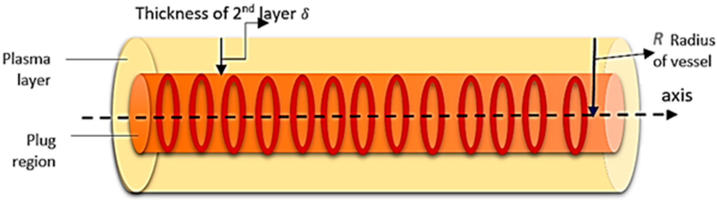
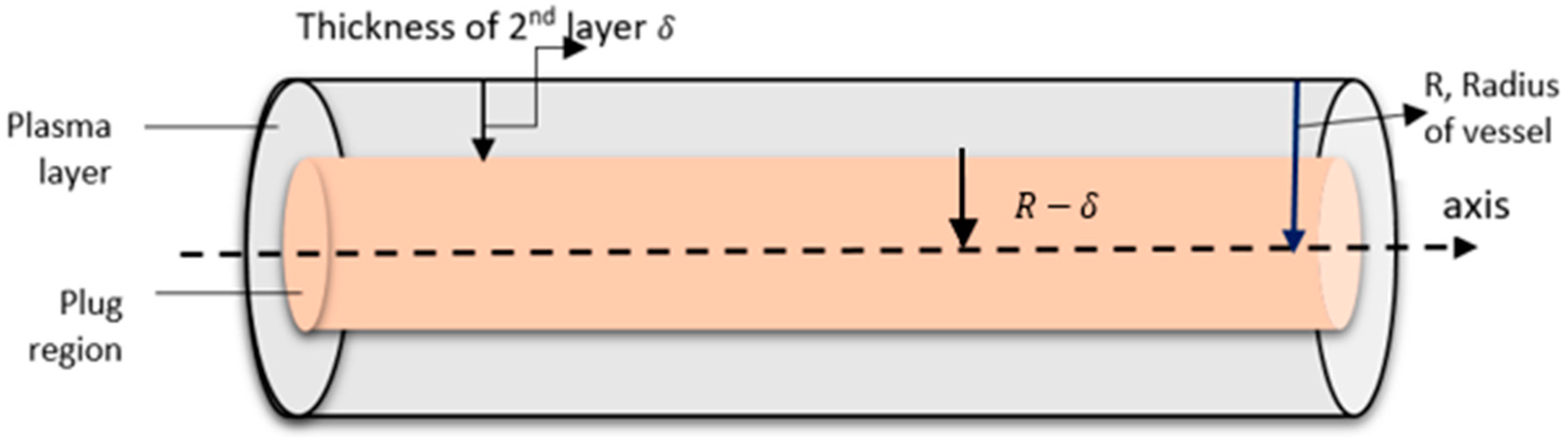
2. Real Model

The whole model of blood flow in the capillary is presented in the following subsections.

2.1. Choice of Frame of Reference

Capillaries have taken approximately cylindrical tubes, although they are not perfectly cylindrical. An orthogonal curvilinear coordinate system is selected for the modeling [30]. All the physical quantities are expressed into tensorial form as biological law holds accurately in the given coordinate system.

2.2. Two-Phase Blood Flow

Let $Y$ be the volume portion covered by the blood in unit volume, and $Y$ can be replaced by $\frac{H_a}{100}$, where $H_a$ is the hematocrit (the volume percentage of blood cells) [3]. Then, the volume portion covered by plasma will be $\left(1-Y\right)$. If the mass ratio of blood cells to plasma is $m_r,$ then

$$m_r=\frac{Y{\rho }_c}{(1-Y){\rho }_p},$$

where ${\rho }_c$ and ${\rho }_p$ are the densities of the blood cells (core layer) and the plasma layer, respectively. Usually, this ratio is not constant; but in the case of the capillary, it is supposed to be constant [31].

2.3. Choice of Parameters

The following quantities are taken as parameters:

(a)

${\mathit{v}}^k=v^k(x^l,t)$; $l=1, 2, 3$; and $k=1, 2, 3$, which is the velocity of blood at a given point $x^l$ in a space at a given time $t$.

(b)

$p=p(x^l,t)$; $l=1, 2, 3$, which is the pressure of blood at a given point $x^l$ in a space at a given time $t$.

2.4. Constitutive Equation

The constitutive equation of the two-layered blood flow model for capillaries is as follows:

$$\begin{gathered} {\mathit{\tau }}^{lk}={\eta }_m\left({\mathit{e}}^{lk}\right)-p{g}^{lk}, \\ \Rightarrow {\mathit{\tau }}^{lk}={\eta }_m\left(g^{ki} {\mathit{v}}_{,i}^l\right)-p{g}^{lk}, \end{gathered}$$

(3)

where ${\eta }_m=Y{\eta }_c+(1-Y){\eta }_p$;${\eta }_m$, ${\eta }_c$, and ${\eta }_p$ are the viscosity of the mixture, core layer, and plasma layer, respectively; and ${\mathit{v}}_{,i}^l$ is the covariant derivative of the velocity tensor [32].

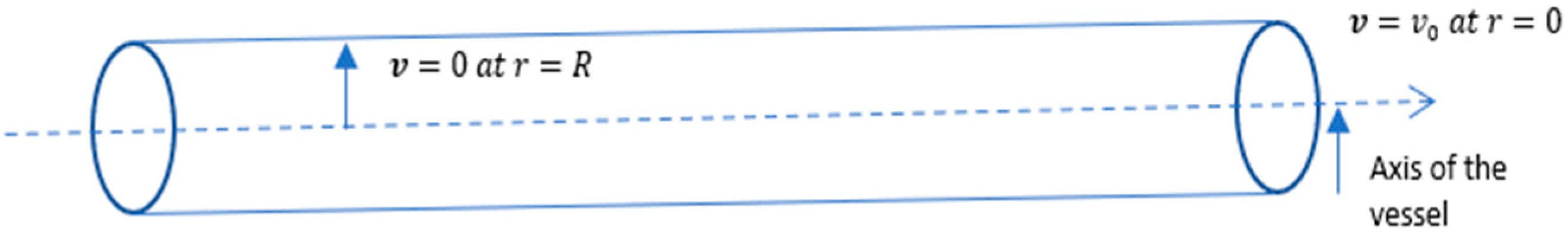
2.5. Boundary Conditions

Two boundary conditions (see Figure 2) have been taken for modeling purposes, given as follows:

(a)

Maximum velocity of blood flow at the axes; i.e., when the radius of vessels is $r=0,$ the velocity of blood flow is at a maximum, $\mathrm{i}.\mathrm{e}., \mathit{v}=v_0$ (say).

(b)

No slip condition (velocity on the boundary is zero); i.e., when theradius is $r=R$, then $\mathit{v}=0$.

3. Mathematical Formulation

The formulation of the proposed problem combines the equation of continuity and the equation of motion. Details are given in following subsections.

3.1. Equation of Continuity

When there is no source and sink in any flowing fluid region, the mass of the fluid is conserved in that region. As there is no source and sink in the human circulatory system [33], the law of conservation of mass can be applied here, which means the mass of blood that enters into the system is equal to the mass of blood that exist outside the system [28].

It is assumed that both phases in the core layer move with common velocity into the capillary. From the principle of conservation of mass, the equation of continuity for RBC phase is given as follows:

$$\frac{\partial \left(Y{\rho }_c\right)}{\partial t}+{\left(Y{\rho }_c{\mathit{v}}^l\right)}_{,l}=0.$$

(4)

The equation of continuity for plasma phase is also given as follows:

$$\frac{\partial (1-Y){\rho }_p}{\partial t}+{\left(\right(1-Y\left){\rho }_p{\mathit{v}}^l\right)}_{,l}=0,$$

(5)

where $\mathit{v}$ is the common velocity of both phases, ${\rho }_c$ and ${\rho }_p$ are densities of core layer and plasma layer, respectively. ${\left(Y{\rho }_c{\mathit{v}}^l\right)}_{,l}$ is a covariant derivative of $\left(Y{\rho }_c{\mathit{v}}^l\right)$ with respect to $X^l$. In the same way, ${\left(\right(1-Y\left){\rho }_p{\mathit{v}}^l\right)}_{,l}$ with respect to $X^l$ [3,34,35].

We define the uniform density ${\rho }_m$ as follows:

$$\frac{1+r_0}{{\rho }_m}=\frac{r_0}{{\rho }_c}+\frac{1}{{\rho }_p}.$$

(6)

Above Equations (4) and (5) can be combined together as follows:

$$\frac{\partial {\rho }_m}{\partial t}+{\left({\rho }_m{\mathit{v}}^l\right)}_{,l}=0.$$

(7)

As we know, blood is an incompressible fluid; hence, ${\rho }_m$ is constant. Thus, the equation of continuity (7) for blood flow takes the following form:

$$\begin{gathered} {\mathit{v}}_{,l}^l=0, \\ \mathrm{i}.\mathrm{e}., \frac{\partial {\mathit{v}}^l}{\partial X^l}+\frac{{\mathit{v}}^l\partial \sqrt{g}}{\sqrt{g}\partial X^l}=0, \\ \Rightarrow \frac{1}{\sqrt{g}}{\left(\sqrt{g}{\mathit{v}}^l\right)}_{,l}=0. \end{gathered}$$

(8)

3.2. Equation of Motion

The total momentum of any system is conserved in the absence of external force. The effect of external force in our human circulatory system is zero in normal situations. So, the law of conservation of momentum can fully apply to this system. The hydrodynamical pressure $p$ between the two phases of blood can be supposed to be uniform because both layers, core and plasma, are always in an equilibrium state in the blood. Now, applying the principle of conservation of momentum, we obtain the equation of motion for the phase of red blood cells as follows [3,34,35]:

$$Y{\rho }_c\frac{\partial {\mathit{v}}^l}{\partial t}+\left(Y{\rho }_c{\mathit{v}}^k\right){\mathit{v}}_{,k}^l=-Y{p}_{,k}{g}^{lk}+Y{\eta }_c{\left(g^{ki}{\mathit{v}}_{,i}^l\right)}_{,k}.$$

(9)

In a similar manner, the equation of motion for plasma in the core layer will be as follows:

$$\left(1-Y\right){\rho }_p\frac{\partial {\mathit{v}}^l}{\partial t}+\left\{\left(1-Y\right){\rho }_p{\mathit{v}}^k\right\}{\mathit{v}}_{,k}^l=-(1-Y)p_{,k}{g}^{lk}+(1-Y){\eta }_p{\left(g^{ki}{\mathit{v}}_{,i}^l\right)}_{,k}.$$

(10)

Now, adding Equations (9) and (10) and using relation (6), the equation of motion for blood flow with the combination of both phases will be reduced as follows:

$${\rho }_m\frac{\partial {\mathit{v}}^l}{\partial t}+\left({\rho }_m{\mathit{v}}^k\right){\mathit{v}}_{,k}^l=-p_{,k}{g}^{lk}+{\eta }_m{\left(g^{ki}{\mathit{v}}_{,i}^l\right)}_{,k},$$

(11)

where ${\rho }_m=Y{\rho }_c+(1-Y){\rho }_p$ is the density and ${\eta }_m=Y{\eta }_c+(1-Y){\eta }_p$ is the viscosity of a mixture of blood (blood cells and plasma), respectively.

Equations (8) and (11) are transformed in cylindrical form.

For cylindrical coordinates, ${ x}^1=r,x^2=\theta , x^3=z$.

Components of metric tensor ${\left[g_{lk}\right]}_{3\times 3}$ are ${ g}_{11}=1, { g}_{22}=r^2, { g}_{33}=1,$ and the rest of the entries are zero.

The determinant of metric tensor is $g=r^2$. The conjugate metric tensor [30] is as follows:

$$g^{lk}=\frac{\mathrm{c}\mathrm{o}\mathrm{f}\mathrm{a}\mathrm{c}\mathrm{t}\mathrm{o}\mathrm{r} \mathrm{o}\mathrm{f} g_{lk}}{g}.$$

Again, components of the conjugate metric tensor are ${ g}^{11}=1, g^{22}=\frac{1}{r^2}, and g^{33}=1$, and the rest of the entries are zero.

Christoffel’s symbol of the second kind, $\mathrm{i}.\mathrm{e}.,\left\{\begin{array}{c}l\\ i j\end{array}\right\}=g^{lk}\left[ij,k\right]=\frac{1}{2}{g}^{lk}\left(\frac{\partial g_{jk}}{\partial x^i}+\frac{\partial g_{ik}}{\partial x^j}-\frac{\partial g_{ij}}{\partial x^k}\right)$, is as follows:

$\left\{\begin{array}{c}1\\ 2 2\end{array}\right\}=-r,\left\{\begin{array}{c}2\\ 2 1\end{array}\right\}=\left\{\begin{array}{c}2\\ 1 2\end{array}\right\}=\frac{1}{r}$, and the rest are zero [30,36].

The relationship between the physical components and contravariant components [30] of the velocity of blood flow are as follows:

$$\begin{gathered} \sqrt{g_{11}}{v}^1=v_r\Rightarrow v_r=v^1, \\ \sqrt{g_{22}}{v}^2=v_{\theta }\Rightarrow {v_{\theta }=rv}^2, \\ \mathrm{and} \sqrt{g_{33}}{v}^3=v_z\Rightarrow v_z=v^3, \\ -p_{,k}{g}^{lk}\Rightarrow -\sqrt{g_{ll}}{p}_{,k}{g}^{lk}. \end{gathered}$$

Now, the governing equations of blood flow are taken in the following form:

Equation of continuity:

$$\frac{1}{r} \frac{\partial \left(r{v}_r\right)}{\partial r}+\frac{1}{r}\frac{\partial v_{\theta }}{\partial \theta }+\frac{\partial v_z}{\partial z}=0.$$

(12)

The equation of motion is given in $r, \theta$, and $z$ components, as below:

$r$ component is

$${\rho }_m\left(\frac{\partial v_r}{\partial t}+v_r\frac{\partial v_r}{\partial r}+\frac{v_{\theta }}{r}\frac{\partial v_r}{\partial \theta }-\frac{{v_{\theta }}^2}{r}+\frac{\partial v_r}{\partial z}\right)=-\frac{\partial p}{\partial r}+{\eta }_m\left(\frac{\partial }{\partial r}\left\{\frac{1}{r}\frac{\partial \left(r{v}_r\right)}{\partial r}\right\}+\frac{1}{r^2}\frac{{\partial }^2{v}_r}{\partial {\theta }^2}-\frac{2}{r^2}\frac{\partial v_{\theta }}{\partial \theta }+\frac{{\partial }^2{v}_r}{\partial z^2}\right);$$

(13)

$\theta$ component is

$${\rho }_m\left(\frac{\partial v_{\theta }}{\partial t}+v_r\frac{\partial v_{\theta }}{\partial r}+\frac{v_{\theta }}{r}\frac{\partial v_{\theta }}{\partial \theta }-\frac{v_r{v}_{\theta }}{r}+v_z\frac{\partial v_{\theta }}{\partial z}\right)=-\frac{1}{r}\frac{\partial p}{\partial \theta }+{\eta }_m\left(\frac{\partial }{\partial r}\left\{\frac{1}{r}\frac{\partial \left(r{v}_{\theta }\right)}{\partial r}\right\}+\frac{1}{r^2}\frac{{\partial }^2{v}_{\theta }}{\partial {\theta }^2}+\frac{2}{r^2}\frac{\partial v_r}{\partial \theta }+\frac{{\partial }^2{v}_{\theta }}{\partial z^2}\right);$$

(14)

$z$ component is

$${\rho }_m\left(\frac{\partial v_z}{\partial t}+v_r\frac{\partial v_z}{\partial r}+\frac{v_{\theta }}{r}\frac{\partial v_z}{\partial \theta }+v_z\frac{\partial v_z}{\partial z}\right)=-\frac{\partial p}{\partial z}+{\eta }_m\left(\frac{1}{r}\frac{\partial }{\partial r}\left\{r\frac{\partial v_z}{\partial r}\right\}+\frac{1}{r^2}\frac{{\partial }^2{v}_z}{\partial {\theta }^2}+\frac{{\partial }^2{v}_{ z}}{\partial z^2}\right).$$

(15)

4. Solution of the Problem

The blood flow is symmetric with respect to the axis of the capillary, i.e.,$\Rightarrow$ $v_{\theta }=0$, and $v_{r }, v_z$, and $p$ are not, depending on $\theta$. Since only one component of velocity along the axis is effective, we have $v_r=0, { v}_{\theta }=0, \mathrm{a}\mathrm{n}\mathrm{d} v_z=v$ (say).

Since the flow is steady, $\frac{\partial p}{\partial t}=\frac{\partial v_r}{\partial t}=\frac{\partial v_{\theta }}{\partial t}=\frac{\partial v_z}{\partial t}=0$ [33].

Hence, the equation of continuity (12) reduces as follows:

$$\frac{\partial v_z}{\partial z}=0\Rightarrow v_z=v\left(r\right).$$

(16)

The transformed equations of motion, along with the $r, \theta$, and $z$ components, are given as follows:

The $r$ component of equation of motion reduces to

$$\begin{gathered} {\rho }_m\times \left(0\right)=-\frac{\partial p}{\partial r}+{\eta }_m\left(0\right), \\ \Rightarrow \frac{\partial p}{\partial r}=0\Rightarrow p=p\left(z\right). \end{gathered}$$

(17)

The $\theta$ component of equation of motion vanishes because blood flow is free from rotation, and applied pressure is in the normal direction.

Similarly, the $z$ component of the equation of motion reduces to

$$\begin{gathered} {\rho }_m{v}_z\left(0\right)=-\frac{\partial p}{\partial z}+{\eta }_m\left[\frac{1}{r}\frac{\partial }{\partial r}\left\{r\frac{\partial v\left(r\right)}{\partial r}\right\}\right], \\ 0=-\frac{\partial p}{\partial z}+{\eta }_m\left[\frac{1}{r}\frac{\partial }{\partial r}\left\{r\frac{\partial v\left(r\right)}{\partial r}\right\}\right], \\ {\eta }_m\left[\frac{1}{r}\frac{d}{dr}\left\{r\frac{dv\left(r\right)}{dr}\right\}\right]=-P, \end{gathered}$$

(18)

where the pressure gradient is

$$-\left(\frac{\partial p}{\partial z}\right)=P.$$

(19)

Now, we solve Equation (18) using boundary conditions $\mathit{v}=v_0 \mathrm{a}\mathrm{t} r=0$ and $\mathit{v}=0$ at $r=R$ (no slip condition) and obtain the velocity of mixture of blood flow, i.e.,

$$\mathit{v}=\frac{P}{4{\eta }_m}\left(R^2-r^2\right).$$

(20)

Therefore, the velocity of the plasma layer (as if the whole capillary was filled with plasma) is

$${\mathit{v}}_{\mathit{p}}=\frac{P}{4{\eta }_p}(R^2-r^2), R-\delta \le r\le R.$$

(21)

Similarly, velocity of the core layer (if core the layer was filled in the whole capillary and the relative velocity of both layers was also added) is

$${\mathit{v}}_{\mathit{m}}=\frac{P}{4{\eta }_m}\left(R^2-r^2\right)+\frac{P}{4{\eta }_m}\left(R^2-{(R-\delta )}^2\right)\left(\frac{{\eta }_m}{{\eta }_p}-1\right), 0\le r\le R-\delta ,$$

(22)

where $R$ is the radius of the capillary and $\delta$ is the thickness of the plasma layer (see in Figure 3) and is supposed to be independent of $R$.

5. Result and Discussion (Biophysical Interpretation)

The flow flux of blood in the capillary [24] is defined as

$$\begin{gathered} Q={\int }_0^{R-\delta }{v}_{m}2\pi r dr+{\int }_{R-\delta }^R{v}_{p}2\pi r dr, \\ ={\int }_0^{R-\delta }\left[\frac{P}{4{\eta }_m}\left(R^2-r^2\right)+\frac{P}{4{\eta }_m}\left(R^2-{(R-\delta )}^2\right)\left(\frac{{\eta }_m}{{\eta }_p}-1\right)\right]2\pi r dr+{\int }_{R-\delta }^R\left[\frac{P}{4{\eta }_p}(R^2-r^2)\right]2\pi r dr. \end{gathered}$$

Using (20) and (21) in the above expression, we obtain

$$Q=\frac{\pi P{R}^4}{8{\eta }_p}\left[1-{\left(1-\frac{\delta }{R}\right)}^4\left(1-\frac{{\eta }_p}{{\eta }_m}\right)\right]$$

(23)

If the whole capillary is supposed to be filled with only one Newtonian blood, whose effective viscosity is ${\eta }_e$, then the flow flux of the blood [24] is

$$Q=\frac{\pi P{R}^4}{8{\eta }_e}.$$

(24)

Comparing Formulae (23) and (24), we obtain the effective viscosity as follows

$${{\eta }_e={\eta }_p\left[1-{\left(1-\frac{\delta }{R}\right)}^4\left(1-\frac{{\eta }_p}{{\eta }_m}\right)\right]}^{-1},$$

(25)

which depends upon the radius $R$ of the capillary. Since $\frac{\delta }{R}\ll \ll 1,$ the Formula (25) can be expanded in the higher power of $\frac{\delta }{R}$, taking first approximation of $\frac{\delta }{R}$; then, it is reduced in the following form:

$${\eta }_e={\eta }_m\left[1-\frac{4\delta }{R}\left(\frac{{\eta }_m}{{\eta }_p}-1 \right)\right].$$

(26)

It is observed from Equation (26) that the effective viscosity decreases with the decrease in the radius of the capillary $R$. Thus, the Fahraeus–Lindqvist effect is explained mathematically.

5.1. Numerical Simulation

A comparison and validation have conducted between the results obtained from the two-phase blood flow model and the experimental data after validation of the results simulated for the human capillary. To validate our model with the experimental result [1], the following numerical values were given to different parameters:

$\delta =\frac{2}{3}R, {\eta }_c=0.0249 \mathrm{P}\mathrm{a}\mathrm{s}\mathrm{c}\mathrm{a}\mathrm{l}\mathrm{s}, {\eta }_p=0.00158-0.00172$ Pascal s, $H_a=11.6-$26 [31]. For validation of the model value of the $R$ taken from the experimental data, it is simulated on a human capillary of 4–10 $\mathsf{\mu }\mathrm{m}$ [3]. MATLAB2020a software is used for numerical simulation and to draw all figures.

$$\begin{gathered} P=\frac{∆p}{∆z}=\frac{\mathrm{p}\mathrm{r}\mathrm{e}\mathrm{s}\mathrm{u}\mathrm{r}\mathrm{e} \mathrm{d}\mathrm{r}\mathrm{o}\mathrm{p}}{\mathrm{l}\mathrm{e}\mathrm{n}\mathrm{g}\mathrm{t}\mathrm{h} \mathrm{o}\mathrm{f} \mathrm{t}\mathrm{h}\mathrm{e} \mathrm{c}\mathrm{a}\mathrm{p}\mathrm{i}\mathrm{l}\mathrm{l}\mathrm{a}\mathrm{r}\mathrm{y}}=\frac{p_f-p_i}{z_f-z_i}, \\ {p}_f=\frac{2}{3}\left(\frac{\frac{S+D}{2}+D}{3}\right)=\mathrm{p}\mathrm{r}\mathrm{e}\mathrm{s}\mathrm{s}\mathrm{u}\mathrm{r}\mathrm{e} \mathrm{a}\mathrm{t} \mathrm{v}\mathrm{e}\mathrm{n}\mathrm{u}\mathrm{l}\mathrm{e}\mathrm{s}, p_i=\frac{\frac{S+D}{2}+D}{3}=\mathrm{p}\mathrm{r}\mathrm{e}\mathrm{s}\mathrm{s}\mathrm{u}\mathrm{r}\mathrm{e} \mathrm{a}\mathrm{t} \mathrm{a}\mathrm{r}\mathrm{t}\mathrm{e}\mathrm{r}\mathrm{i}\mathrm{o}\mathrm{l}\mathrm{e}\mathrm{s}, \\ S\le 110 \mathrm{m}\mathrm{m}\mathrm{h}\mathrm{g}\left(\mathrm{S}\mathrm{y}\mathrm{s}\mathrm{t}\mathrm{o}\mathrm{l}\mathrm{i}\mathrm{c} \mathrm{p}\mathrm{r}\mathrm{e}\mathrm{s}\mathrm{s}\mathrm{u}\mathrm{r}\mathrm{e}\right),\hspace{0.17em}D\le 70 \mathrm{m}\mathrm{m}\mathrm{h}\mathrm{g}=(\mathrm{D}\mathrm{i}\mathrm{a}\mathrm{s}\mathrm{t}\mathrm{o}\mathrm{l}\mathrm{i}\mathrm{c} \mathrm{p}\mathrm{r}\mathrm{e}\mathrm{s}\mathrm{s}\mathrm{u}\mathrm{r}\mathrm{e}). \end{gathered}$$

Table 1. Experiment Series 1, Torsten Lindqvist (T.L.).

Series 1
$\mathbf{Relative} \mathbf{Viscosity} \mathbf{of} \mathbf{Plasma} {\mathit{\eta }}_{\mathit{p}}=1.63\times {10}^{-3}\hspace{0.17em}\mathbf{P}\mathbf{a}\mathbf{s}\mathbf{c}\mathbf{a}\mathbf{l}-\mathbf{S}$
S. No.	Length of Tube (m)	Diameter (m)	Relative Viscosity (Pascal-S)
1	0.1265	$5.05\times {10}^{-4}$	$4.60\times {10}^{-3}$
2	0.1210	$3.11\times {10}^{-4}$	$4.54\times {10}^{-3}$
3	0.0456	$1.75\times {10}^{-4}$	$4.22\times {10}^{-3}$
4	0.0500	$1.20\times {10}^{-4}$	$3.98\times {10}^{-3}$
5	0.0326	$8.10\times {10}^{-5}$	$3.65\times {10}^{-3}$
6	0.0118	$6.50\times {10}^{-5}$	$3.38\times {10}^{-3}$
7	0.0118	$4.70\times {10}^{-5}$	$2.95\times {10}^{-3}$
8	0.0126	$4.00\times {10}^{-5}$	$2.79\times {10}^{-3}$

,

Table 2. Experiment Series 2, Torsten Lindqvist (T.L.).

Series 2
$\mathbf{Relative} \mathbf{Viscosity} \mathbf{of} \mathbf{Plasma} {\mathit{\eta }}_{\mathit{p}}=1.65\times {10}^{-3}\hspace{0.17em}\mathbf{P}\mathbf{a}\mathbf{s}\mathbf{c}\mathbf{a}\mathbf{l}-\mathbf{S}$
S. No.	Length of Tube (m)	Diameter (m)	Relative Viscosity (Pascal-S)
1	0.1255	$2.77\times {10}^{-4}$	$4.96\times {10}^{-3}$
2	0.0456	$1.75\times {10}^{-4}$	$4.54\times {10}^{-3}$
3	0.0500	$1.20\times {10}^{-4}$	$4.22\times {10}^{-3}$
4	0.0118	$4.70\times {10}^{-5}$	$3.98\times {10}^{-3}$

,

Table 3. Experiment Series 3, Robin Fahraeus (R.F.).

Series 3
$\mathbf{Relative} \mathbf{Viscosity} \mathbf{of} \mathbf{Plasma} {\mathit{\eta }}_{\mathit{p}}=1.60\times {10}^{-3}\hspace{0.17em}\mathbf{P}\mathbf{a}\mathbf{s}\mathbf{c}\mathbf{a}\mathbf{l}-\mathbf{S}$
S. No.	Length of Tube (m)	Diameter (m)	Relative Viscosity (Pascal-S)
1	----	$4.60\times {10}^{-4}$	$5.21\times {10}^{-3}$
2	0.1000	$2.77\times {10}^{-4}$	$5.10\times {10}^{-3}$
3	0.0850	$1.05\times {10}^{-4}$	$4.28\times {10}^{-3}$
4	----	$5.20\times {10}^{-5}$	$3.52\times {10}^{-3}$

and

Table 4. Experiment Series 4, Torsten Lindqvist (T.L.).

Series 4
$\mathbf{Relative} \mathbf{Viscosity} \mathbf{of} \mathbf{Plasma} {\mathit{\eta }}_{\mathit{p}}=1.72\times {10}^{-3}\hspace{0.17em}\mathbf{P}\mathbf{a}\mathbf{s}\mathbf{c}\mathbf{a}\mathbf{l}-\mathbf{S}$
S. No.	Length of Tube (m)	Diameter (m)	Relative Viscosity (Pascal-S)
1	0.1225	$2.77\times {10}^{-4}$	$6.80\times {10}^{-3}$
2	0.0456	$1.75\times {10}^{-4}$	$6.28\times {10}^{-3}$
3	0.0500	$1.20\times {10}^{-4}$	$5.59\times {10}^{-3}$
4	0.0279	$8.10\times {10}^{-5}$	$5.08\times {10}^{-3}$
5	0.0070	$6.50\times {10}^{-5}$	$4.71\times {10}^{-3}$
6	0.0118	$4.70\times {10}^{-5}$	$4.28\times {10}^{-3}$

for different series have been taken from the experimental data [1]. Series 1, 2, and 4 of the experiments were given by Torsten Lindqvist, and Series 3 was given by Robin Fahraeus, shown below.

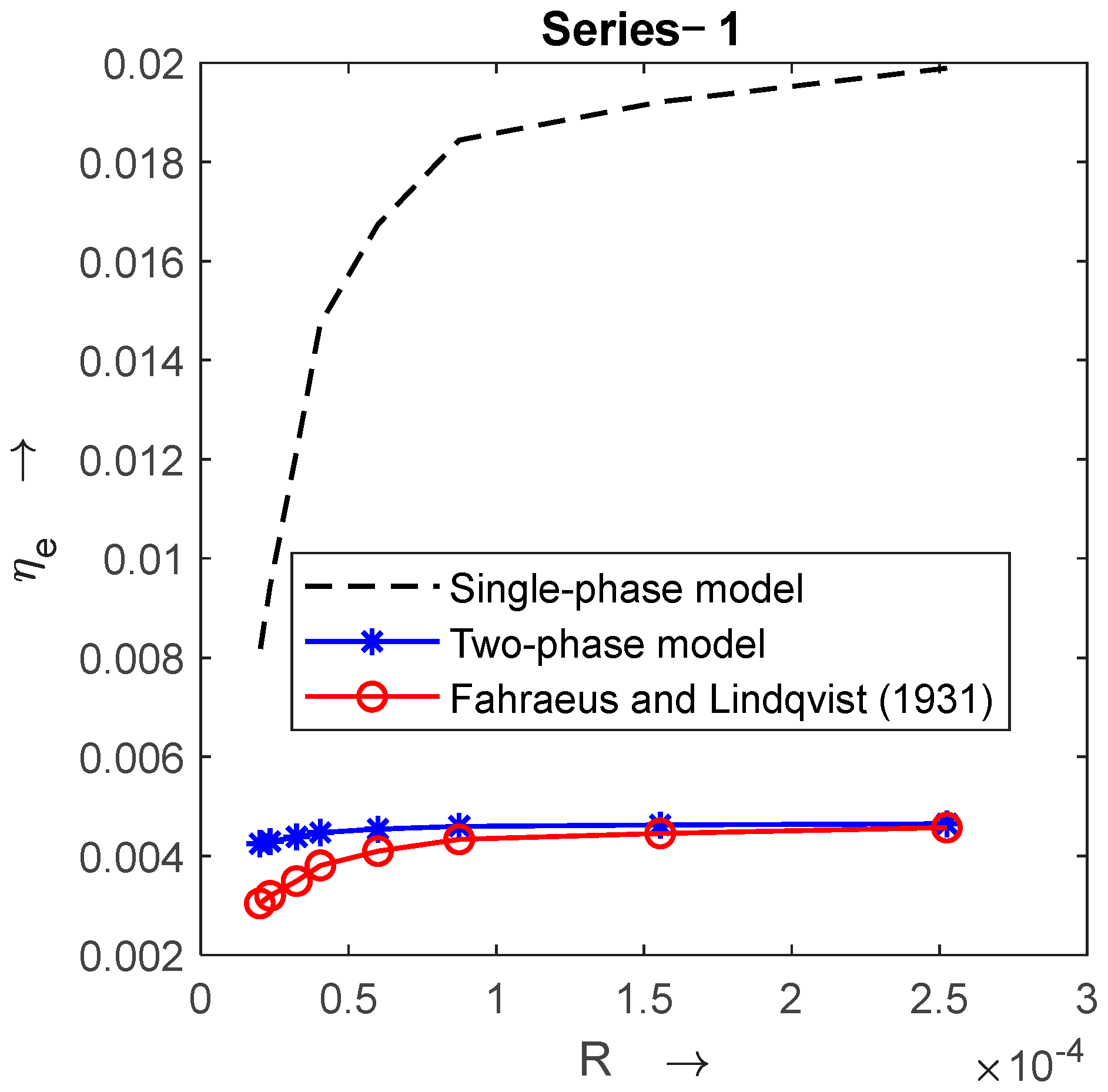
5.2. Validation of Two-Phase Blood Flow Model

Figure 4 shows the graph between ${\eta }_e$ and $R$. The effective viscosity ${\eta }_e$ is obtained from a single-phase model (from Equation (1)), a two-phase-model (from Equation (26)), and the experimental data of series-1. For $H_a$ = 15.6, the two-phase model is much closer to the experimental data in Series 1 than the single-phase model. So next, the impact of different physiological parameters relevant to the flow, with help of the two-phase blood flow model, was analyzed.

Figure 5 shows variation in ${\eta }_e$ and $R$, which are obtained from the two-phase blood flow model and experimental Series 1 to 4. In the figures of each series, ${\eta }_e$ decreases with radius $R$. For $H_a=$15.6, 18.2, 19.8, and 27.6, the proposed model is much closer to the experimental Series 1, 2, 3, and 4, respectively (see Figure 5).

The proposed two-phase blood flow model gives a better approximation than the single-phase blood flow model. This model will be used for further studies on the human capillary. The internal diameter of the capillary lies between 4 and 10 $\mathsf{\mu }\mathrm{m}$ [3]. For this purpose, a capillary with radius $R=5 \mathsf{\mu }\mathrm{m}$, length $\Delta z=6 \mathsf{\mu }\mathrm{m}$, and thickness of plasma layer $\delta =\frac{2}{3}R$ was used [37].

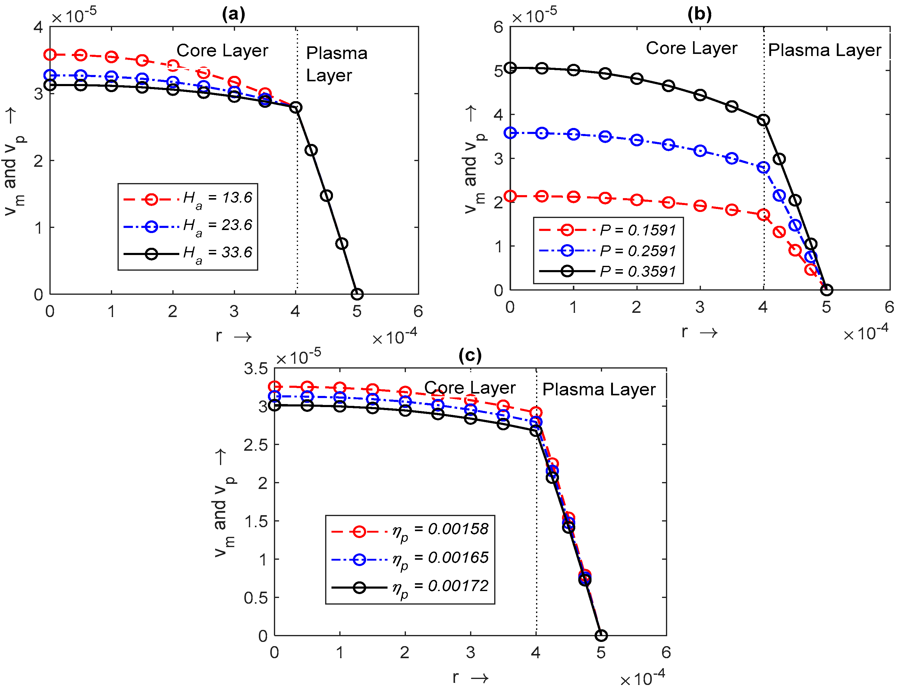
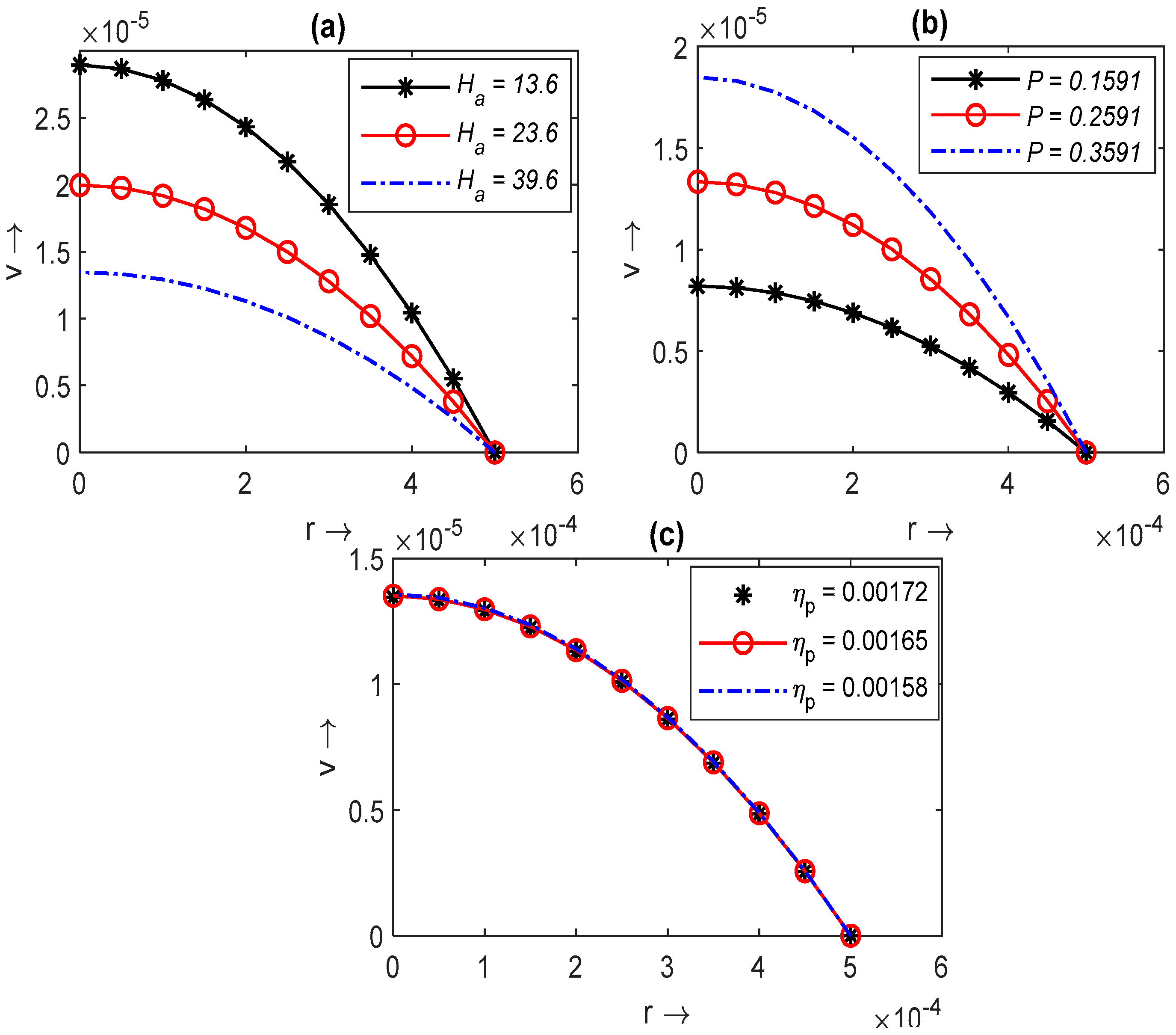
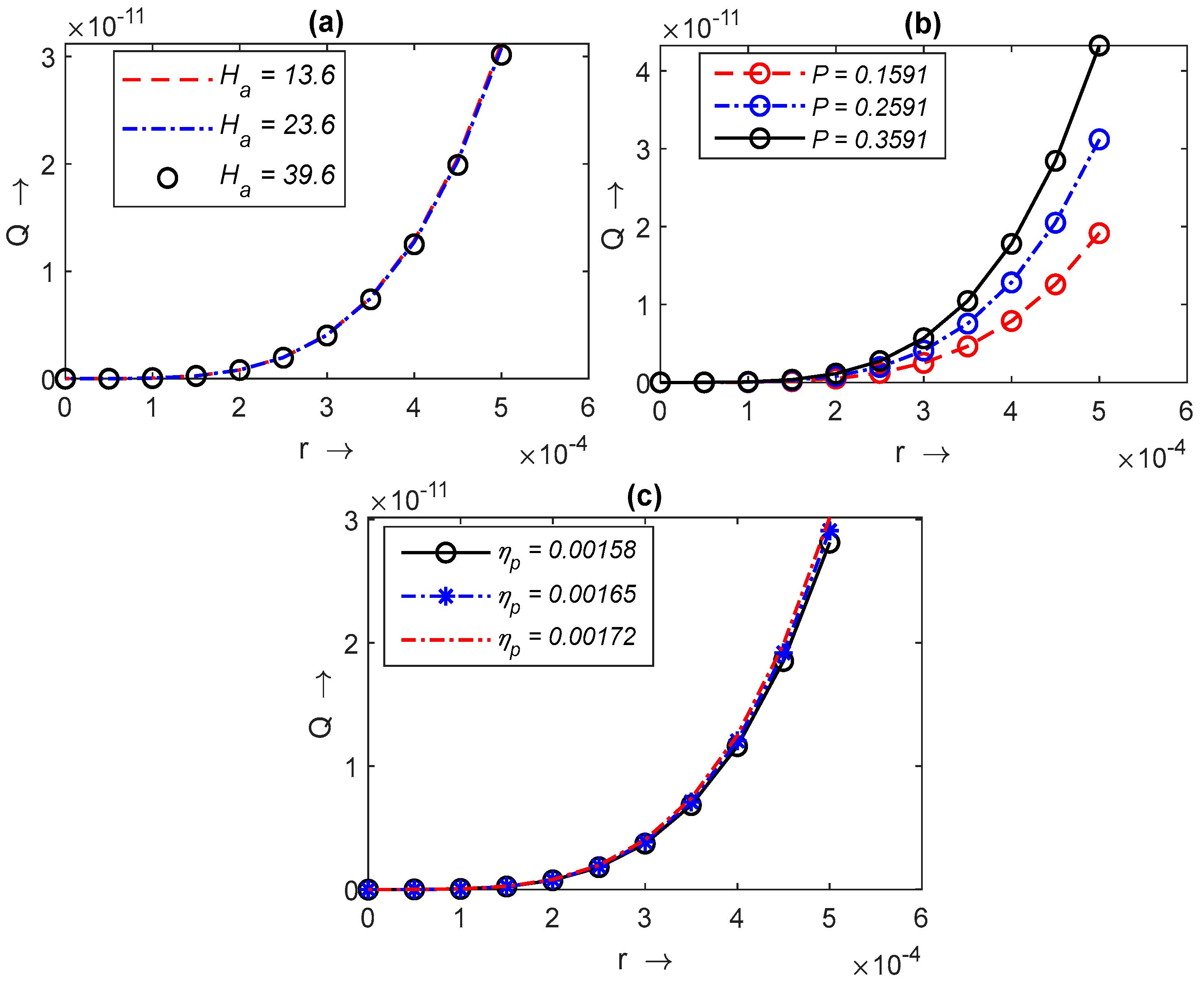
5.3. Effect of $H_a,{\eta }_p$, and $P$ on ${\eta }_e$

For a capillary F-L effect, as shown in Figure 6a–c, the radii were taken from $0<r\le R$. ${\eta }_e$ decreases rapidly in the capillary with a radius less than $3 \mathsf{\mu }\mathrm{m}$. In Figure 6a,b, ${\eta }_e$ decreases with decreasing values of $r$. Figure 6a shows variation in ${\eta }_e$ with radius $0<r\le R$ for different values of $H_a$. From Figure 6a, it is observed that ${\eta }_e$ decreases with the higher concentration of $H_a$. The concentration of RBC in the capillaries increases but it decreases ${\eta }_e$ along with $r$; hence, flow is possible. Figure 6b shows the impact of ${ \eta }_p$ on ${\eta }_e$; it decreases with higher values of viscosity of the plasma layer. Figure 6c shows the impact of pressure drop $P$ on ${\eta }_e$. It is assumed that the capillaries are far away from the heart and proximate to the tissue; hence, its pumping effect has been negligible. This effect can also be seen in Figure 6c. Increasing the value of $P$ does not much affect ${\eta }_e$.

5.4. Effect of $H_a,$${\eta }_p$, and $P$ on $v,v_m, and v_p$

The velocity profile $v$ for the mixture of blood is shown in Figure 7a–c. In each figure $, v$ increases with the decreasing radius of the capillary, tending to zero at $r=R$. Figure 7a shows the effect of ${ H}_a$ on $v$. It can be observed from Figure 7a that a higher volume percentage of RBC decreases $v$. The impact of pressure drop $P$ on whole blood is shown in Figure 7b. Although the heart pumping effect in not very effective into the capillaries, its larger value increases blood velocity. Figure 7c shows the effect of plasma viscosity on $v$. ${\eta }_p$ slightly affects velocity $v$. Higher values of ${\eta }_p$ decrease $v$, but they do not greatly influence it.

Blood is separated into two layers when it flows from the capillary. Graphs of combined velocity profiles have been plotted for the core layer $v_m$ (for radius $0\le r\le R-\delta$) and the plasma layer $v_p$ $\left(R-\delta \le r\le R\right)$ (see Figure 8a–c). Figure 8a shows the impact of the volume percentage of RBC on both layers. As the plasma layer is free from RBC, which flows near the wall of the capillary, the impact of $H_a$ cannot be seen in the velocity profile of the plasma layer. Its effect can be seen only on the core layer. $v_m$ decreases as $H_a$ increases. The pressure drop also increases the velocity of both layers (see Figure 8b). The impact of the viscosity of the plasma layer on both layers is shown in Figure 8c. The velocity of both layers increases as plasma viscosity decreases.

5.5. Effect of $H_a,{\eta }_p$, and $P$ on $Q$

Variation in $Q$ with respect to radius $r$ is shown in Figure 9a–c. In each figure, $Q$ decreases rapidly with the decreasing radius $r$, and after the radius $2 \mathsf{\mu }\mathrm{m}$ changes in $Q$ cannot be seen explicitly; it becomes stable for radii less than $2 \mathsf{\mu }\mathrm{m}$. The impact of $H_a$ is shown in Figure 9a. The graphs between $Q$ and $r$ for different values of $H_a$ overlap, which that means $Q$ is not much affected by ${ H}_a$. Figure 9b shows the effect of the pressure drop on $Q$. Increasing values of $P$ also increase $Q$, but for radii less than $2 \mathsf{\mu }\mathrm{m}$, the curves coincide, which means that for small- radius vessels, changes in $Q$ become static. Figure 9c shows the impact of plasma viscosity on $Q$. The effect of ${\eta }_p$ on $Q$ can be seen explicitly for the vessel with a radius larger than $2 \mathsf{\mu }\mathrm{m}$. $Q$ increases as ${ \eta }_p$ decreases, but for a radius less than $2 \mathsf{\mu }\mathrm{m}$, $Q$ does not change as much.

Figure 8. Variation in $v_m$ with radius $(0\le r\le R-\delta )$ and $v_p$ with radius $(R-\delta \le r\le R)$, respectively, for different values of (a) hematocrit $H_a$, (b) pressure drop $P$, and (c) plasma viscosity ${\eta }_p$.

Figure 8. Variation in $v_m$ with radius $(0\le r\le R-\delta )$ and $v_p$ with radius $(R-\delta \le r\le R)$, respectively, for different values of (a) hematocrit $H_a$, (b) pressure drop $P$, and (c) plasma viscosity ${\eta }_p$.

6. Conclusions

A two-phase microcirculation model that explains the F-L effect has been presented here. For the validation of the model, the obtained results are compared with the experimental data and single-phase blood flow model, respectively. Further, we simulated these results on the human capillary. The effects of various physiological parameters have been shown through different graphs. We present the conclusions of this study as follows:

• A mathematical expression has been obtained between ${\eta }_e$ and $R$ which successfully explains the F-L effect.
• We have obtained effective, rather than apparent, viscosity.
• With the help of this model, extension of Haynes theory is possible because for the relative momentum of RBC, the plasma is mixed in the core layer, and both phases are homogeneously distributed in the core layer.
• Experimental data and the results obtained from the presented model have the same trends, but this model provides an extension of the F-L effect.
• The presented model successfully explains all the physical phenomena which occur in the capillary.
• The flow flux and velocity of the blood decreases in the capillary due to the higher concentration of $H_a$, but flow is possible because effective viscosity decreases as the radius of the capillary decreases.
• The pressure gradient can increase the effective viscosity and flow flux, but it is not very effective in terms of blood flowing into capillaries as they are remote from the heart and proximate to the human tissue.

There are several two-phase blood flow models of the F-L effect, but uses of tensors and the RBCs of the core layer considered are liquid in form and packed in a semipermeable membrane, capable of changing its shape and size, which demonstrates the nature of the liquid, not of a suspended particle, moving the model closer to the reality. This model not only successfully explains the F-L effect but is also able to determine the impact of several physiological parameters on blood flow in the capillary.

References

- Fahraeus, R.; Lindqvist, J.T. The viscosity of the blood in narrow capillary tubes. Am. J. Physiol. 1931, 96, 562–568. [Google Scholar] [CrossRef]
- Wilson, R. Anatomy and Physiology in Health and Illness, 11th ed.; Churchill Livingstone: London, UK, 2014. [Google Scholar]
- Guyton, A.C.; Hall, J.E. Textbook of Medical Physiological, 11th ed.; Elsevier Inc.: New Delhi, India, 2006. [Google Scholar]
- Dalkara, T. Cerebral Microcirculation: An Introduction; Springer: Berlin/Heidelberg, Germany, 2015; pp. 655–680. [Google Scholar]
- Cipolla, M.J. The Cerebral Circulation; Morgan and Claypool Life Sciences: San Rafael, CA, USA, 2009; ISBN 9781615040131. [Google Scholar]
- Toksvang, L.N.; Berg, R.M.G. Using a classic paper by Robin Fåhræus and Torsten Lindqvist to teach basic hemorheology. Adv. Physiol. Educ. 2013, 37, 129–133. [Google Scholar] [CrossRef] [PubMed]
- Secomb, T.W.; Pries, A.R. Blood viscosity in microvessels: Experiment and theory. C. R. Phys. 2013, 14, 470–478. [Google Scholar] [CrossRef] [PubMed]
- Martini, P.; Pierach, A.; Scheryer, E. Die stromung des blutes in engen gefäßen. Eine abweichung vom poiseuille’schen gesetz. Dtsch. Arch. Klin. Med. 1931, 169, 212–222. [Google Scholar]
- Pries, A.R.; Neuhas, D.; Gaehtgens, P. Blood viscosity in tube flow: Dependence on diameter and hematocrit. Am. J. Physiol. Heart Circ. Physiol. 1992, 263, H1770–H1778. [Google Scholar] [CrossRef] [PubMed]
- Haynes, R.F. Physical basis of the dependence of blood viscosity on tube radius. Am. J. Physiol. 1960, 198, 1193–1200. [Google Scholar] [CrossRef] [PubMed]
- Botkin, N.D.; Kovtanyuk, A.E.; Turova, V.L.; Sidorenko, I.N.; Lampe, R. Accounting for tube haematocrit in modeling of blood flow in cerebral capillary networks. Comput. Math. Methods Med. 2019, 2019, 4235937. [Google Scholar] [CrossRef] [PubMed]
- Sharan, M.; Popel, A.S. A two-phase model for flow of blood in narrow tubes with increased effective viscosity near the wall. Biorheology 2001, 38, 415–428. [Google Scholar] [PubMed]
- Ascolese, M.; Farina, A.; Fasano, A. The Fåhræus-Lindqvist effect in small blood vessels: How does it help the heart. J. Biol. Phys. 2019, 45, 379–394. [Google Scholar] [CrossRef]
- Chebbi, R. Dynamics of blood flow: Modeling of the Fåhræus–Lindqvist effect. J. Biol. Phys. 2015, 41, 313–326. [Google Scholar] [CrossRef]
- Chebbi, R. Dynamics of blood flow: Modeling of Fahraeus and Fahraeus-Lindqvist effects using a shear-induced red blood cell migration model. J. Biol. Phys. 2018, 44, 591–603. [Google Scholar] [CrossRef] [PubMed]
- Chebbi, R. A two-zone shear-induced red blood cell migration model for blood flow in microvessels. Front. Phys. 2019, 7, 206. [Google Scholar] [CrossRef]
- Farina, A.; Rosso, F.; Fasano, A. A Continuum mechanics model for the Fahraeus-Lindqvist effect. J. Biol. Phys. 2021, 47, 253–270. [Google Scholar] [CrossRef] [PubMed]
- Farina, A.; Fasano, A.; Rosso, F. Mathematical models for some aspects of blood microcirculation. Symmetry 2021, 13, 1020. [Google Scholar] [CrossRef]
- Possenti, L.; Di Gregorio, S.; Gerosa, F.M.; Raimondi, G.; Casagrande, G.; Costantino, M.L.; Zunino, P. A computational model for microcirculation including Fahraeus-Lindqvist effect, plasma skimming and fluid exchange with the tissue interstitium. Int. J. Numer. Methods Biomed. Eng. 2019, 35, e3165. [Google Scholar] [CrossRef] [PubMed]
- Wang, T.; Xing, Z. Characterization of blood flow in capillaries by numerical simulation. J. Mod. Phys. 2010, 1, 349. [Google Scholar] [CrossRef]
- Medvedev, A.E.; Fomin, V.M. Two-phase blood-flow model in large and small vessels. Dokl. Phys. 2011, 56, 610–613. [Google Scholar] [CrossRef]
- Medvedev, A.E. Two-phase blood-flow model. Russ. J. Biomech. 2013, 17, 18–32. [Google Scholar]
- Bagchi, P. Mesoscale simulation of blood flow in small vessels. Biophys. J. 2007, 92, 1858–1877. [Google Scholar] [CrossRef]
- Kapoor, J.N. Mathematical Models in Biology and Medicine; E.W.P.: New Delhi, India, 1992; ISBN 8185336822. [Google Scholar]
- Debnath, L. On a micro-continuum model pulsatile blood flow. Acta Mech. 1976, 24, 165–177. [Google Scholar] [CrossRef]
- Devi, G.; Devanathan, R. Peristaltic motion of a micropolar fluid. Proc. Indian Acad. Sci. 1975, 81, 149–163. [Google Scholar] [CrossRef]
- Upadhyay, V.; Chaturvedi, S.K.; Upadhyay, A. A mathematical model on effect of stenosis in two phase blood flow in arteries remote from the heart. Int. Acad. Phys. Sci. 2012, 16, 247–257. [Google Scholar]
- Fung, Y.C. Biomathematics Mechanical Properties of Living Tissues; Springer: New York, NY, USA, 1981; pp. 118–182. [Google Scholar]
- Sherman, I.W.; Sherman, V.G. Biology—A Human Approach; Oxford University Press: New York, NY, USA; Oxford, UK, 1989; pp. 276–277. [Google Scholar]
- Murray, R.S. Vector Analysis and an Introduction to Tensor Analysis; Schaum’s Outline Series; McGraw-Hill: New York, NY, USA, 2021. [Google Scholar]
- Maurya, P.; Upadhyay, V.; Chaturvedi, S.K.; Kumar, D. Mathematical study and simulation on stenosed carotid arteries with the help of two-phase blood flow model. Can. J. Chem. Eng. 2023, 101, 5468–5481. [Google Scholar] [CrossRef]
- De, U.C.; Abosos, S.A.; Joydeep, G.S. Tensor Calculus, 2nd ed.; Alpha Science International, Ltd.: Oxford, UK, 2008. [Google Scholar]
- Landau, L.D.; Lipchitz, E.M. Fluid Mechanics; Pergamon Press: Oxford, UK, 1959. [Google Scholar]
- Wiat, L.; Fine, J. Applied Bio Fluid Mechanics; McGraw-Hill Companies: New York, NY, USA, 2007. [Google Scholar]
- Mazumdar, J.N. Bio Fluid Mechanics; World Scientific: Singapore, 2004. [Google Scholar]
- Spain, B. Tensor Calculus: A Concise Course; Courier Corporation: North Chelmsford, MA, USA, 2003. [Google Scholar]
- Batra, S.; Rakusan, K. Capillary length, tortuosity, and spacing in rat myocardium during cardiac cycle. Am. J. Physiol.-Heart Circ. Physiol. 1992, 263, H1369–H1376. [Google Scholar] [CrossRef]