Study of Non-Smooth Symmetry Collision of Rolling Bodies of Localized Functional-Slot Cage-Less Ball Bearings Considering Lubrication Flow

Abstract

This article presents a vibration model of neighboring rolling parts that takes into account non-smooth symmetric collisions. This model was used to examine the motion state of the rolling element and the collision force between nearby rolling elements. It also determined the motion posture and overall collision form of the rolling element after setting the functional slot. Afterwards, the level of disorderly movement and the structure of the moving object were examined and confirmed through the use of a phase diagram of the motion system in relation to zero symmetry, the Lyapunov exponent, and a platform for measuring irregular vibrations in the bearing. This work aims to clarify the factors that contribute to the persistent chaotic state of rolling elements in bearing vibration.

1. Introduction

Researchers have increasingly focused on cage-free ball bearings as a better alternative to conventional bearings for protecting active magnetic bearings (AMBs). They have conducted studies comparing the performance of cage-free bearings with conventional bearings, specifically examining the differences in their smoothness of operation. Helfert [1] conducted an investigation into the correlation between the rotational motion of a rolling body and the stability of the inner ring in the presence of non-smooth behavior. The study involved using high-speed photography and image recognition technology to precisely determine the positions of the rolling body and the inner ring while the rotor was rotating at a frequency of 150 Hz. At a frequency of 150 Hz, the utilization of high-speed photography technology and image recognition technology allows for the calibration of the position of the rolling body and the inner ring. It has been observed that the bearing operation is unstable due to the fact that the time required for the rolling body to achieve rotational movement stabilization is three times longer than that needed for the inner ring.A Japanese bearing company [2] developed a unique raceway shape with a cage function for cage-free ball bearings. Through a series of performance tests, it was found that the new type of bearing requires significantly less torsional torque compared to conventional ball bearings and exhibit relatively high temperature resistance. However, no detailed analysis of the underlying mechanism or supporting evidence was provided. Nie Aonan [3] conducted an experimental study on the mechanism of non-smooth behavior induced by ball bearing collisions in the absence of a cage. The findings indicate that frictional heat generated in the bearing’s inner ring can cause contact deformation, resulting in relative sliding between the rolling elements and the raceway. Ultimately, this leads to bearing failure. Halmine and other scholars [4,5] conducted a study on the impact of surface fluctuation on the irregular behavior of bearings. They developed a mathematical model that considers friction loss and has two degrees of freedom for the rolling elements. By solving the algorithms, they discovered a significant correlation between the non-smooth behavior of bearings and the speed of the rolling elements relative to the raceway. In comparison to conventional ball bearings, cage-free ball bearings exhibit greater stability and less irregular behavior during the deceleration stage. Kärkkäinen [6] introduced a model to explain the damping of uneven normal contact between rolling elements and raceways in cage-free ball bearings. The model takes into account rotor dropping and investigates the factors causing non-smooth behaviors in this contact. The model is divided and solved using the Runge–Kutta method.

Neisi [7] developed a two-degree-of-freedom spring damping model to analyze the radial direction vibration characteristics of cage-free bearings caused by rotor impact. This model, combined with the Hertzian contact theory, describes the internal contact between the rolling body and the raceway of cage-free ball bearings. The study revealed that the radial force applied to the inner ring by the rolling body became unevenly distributed after the rotor drop. This resulted in concentrated stresses, leading to an increase in local deformation of the bearing raceway and causing instability in the bearing’s operation. SUN [8] conducted a study on the correlation between the stiffness of cage-free bearings and the dynamic distribution of rolling body rotation. They [9] also analyzed the vibration eigenvalues of the inner ring to understand the causes of instability induced by the contact stiffness model. This research offers valuable insights for the development of cage-free bearings. Cage ball bearings [10] can serve as protective bearings for active magnetic bearings (AMBs) and offer a theoretical foundation. The occurrence of non-smooth behavior in the theoretical characterization of and actual research on the impact on the inner ring of the bearing due to the rotor drop can be attributed to the absence of a cage in the ball bearings. The study’s findings indicate that an uneven distribution of rolling parts can cause an unbalanced mass distribution in the rotor system over time, leading to non-smooth behavior. Cole [11] examined the impact of the inner ring system’s stability in cage-less ball bearings and the effect of load changes on friction caused by impacts during the rotor-lowering process. Cole utilized a suitable analytical model to define the cage-less ball bearings. Katarzyna Peta [12] examines the effects of discharge energy on surface micro-texture, chemical composition, contact angle, and surface free energy and compares them. The examination of how lubrication behaves on surfaces with micro-textures in contact mechanics plays a significant role in determining the tribological properties. The research findings validate the efficacy of utilizing bioinspired lubricants to mimic the precise wettability of implant surfaces. Zhil’nikov [13] proposed a method for calculating the friction moment of cage-free ball bearings under axial preload by utilizing the traditional raceway control rolling element theory. This method involves considering the change in the contact angle and the contact elliptic parameter. The friction moment of cage-free ball bearings under different axial loads was determined through experimental calculations and compared. The maximum torque generated by a cage-free ball bearing during operation was examined.

Townsend [14] conducted an experimental analysis to determine the cause of non-smooth frictional resistance in cage-free ball bearings. The results indicated that when the rolling elements are initially distributed uniformly, the non-smooth frictional resistance arises from the movement of the lubricant and the sliding motion between the rolling elements and the raceways. Jones [15] conducted research to determine the service life of cage-free ball bearings in a vacuum environment. The study focused on measuring the friction torque of the bearings and aimed to broaden the range of applications for cage-free ball bearings. Kingsbury [16] utilized high-speed object capture and image recognition technology to analyze the motion deflection of cage-free ball bearings. They discovered that the rotational deflection of the rolling body in cage-free ball bearings is significantly smaller compared to conventional ball bearings. This observation was made under specific conditions in a particular workplace. Ball bearings exhibit a high level of stability when subjected to specific operating conditions. Li Yanfu [17] conducted a study on the pure rolling mechanism of cage-free ball bearings. In this study, he introduced the concept of axial friction angle and developed a calculation model based on this angle to determine the size of the axial friction angle in relation to the rolling body axis and radial non-smoothness. Through this research, he demonstrated that the use of radial clearance and the raceway bus can restrict the unnecessary displacement of the rolling body. Yang Jun [18] conducted a study on the dynamics of friction in water-lubricated bearings. The study focused on the impact of transverse vibration and examined how different excitation amplitudes affect bearing friction. Additionally, the research explored the mechanism of friction-induced vibration in water-lubricated bearings when subjected to elastic deformation conditions. Liu Tengfei [19] discovered that various weaving techniques have varying effects on the thermal fluid properties of bearings. Specifically, low-eccentricity rectangular weaving demonstrates superior lubrication performance. Additionally, the temperature at which oil is introduced into the bearings has a significant influence on their thermal fluid properties. As the oil inlet temperature increases, the characteristics of the bearings gradually deteriorate, although the rate of deterioration slows down. Zhang Ganbo [20] devised a method for analyzing frictional nonlinear vibration systems. This method allows for numerical simulation of step sinusoidal excitation tests to calculate the time–domain response in swept-frequency conditions. By conducting spectral analysis on the obtained response, the frequency response of frictional acceleration can be determined, enabling investigation into the effects of friction. Li Zhongyang [21] discovered that changes in friction have an impact on the size of fluid particles and the surface morphology. The number of particles in the fluid increases due to the wear of the inner ring caused by friction changes, leading to a positive feedback loop that amplifies the amplitude of the wear and further worsens the condition of the bearings.

Adamczak [22] thinks that only two-dimensional morphology parameters are not enough to explain the surface morphology of lubrication in a bearing raceway. Using a lot of measurements of the lubrication surface of rolling bearings along with the dynamic vibration results of rolling elements, three-dimensional morphology parameters need to be used in the theoretical research process to give a more detailed description of the surface morphology of raceway lubrication. This will help the research results be more accurate. Zheng Guogang from Southwest Jiaotong University [23] used ABAQUS 2021 simulation software to look at how stress was distributed in the contact positions between different rolling bearing parts. He then created a three-dimensional lubrication model of the bearing parts and used this to guess how long the bearings would last before they broke. The outer raceway of airplane engine bearings was studied by Yang Jinglai [24]. He used lubricating oil spectroscopy, portable ferrography, analytical ferrography, and energy spectrum analysis. He looked at the rough particles in the rubbing oil inside of the bearings and discovered that the outer ring of the ball bearing slowly peeled off and grew bigger. Luo Maolin [25] looked at how the contact between the rolling element and the lubrication area changes over time in terms of displacement vibration. They found the rolling element’s bearing system energy at both ends of the lubrication area. This allowed them to obtain the rolling element’s force and lubrication length models that affect the lubrication area. The lubrication function was added to the dynamic equation, and a dynamic model for bearing lubrication effect was created. The study found that the bearing’s shaking amplitude showed a double impact effect when the rolling element entered and left the lubrication area.

Imran [26] suggested a research method using dimensional amplitude response analysis and scaling rules. This method takes into account the parameters of the bearing’s lubrication volume and the lubrication area’s surface area when figuring out how to lubricate different parts of a rotor bearing system that is scaled in terms of dimensions. In his study [27], Lu Yang modeled and simulated the lubrication fault dynamics of deep slot ball bearings. He accomplished this by adding the geometric factors of the lubrication area to the well-known model of single-point fault-bearing dynamics. Smith [28] suggested changing the vibration signal in the area of local lubrication into a pulse excitation signal and the lubrication factor into a rolling element pulse signal for modeling bearing dynamics. This was performed after carefully looking at how bearing geometry, speed, combined load, and vibration attenuation affect the signal. Fan [29] figured out how lubrication affects the extra contact deformation of rolling bearings by looking at the uneven internal forces that happen when the inner and outer raceways of the bearings are oiled. He then set up a six-degree-of-freedom vibration differential model. It was found that the uneven forces caused by lubricating the inner and outer raceways have a big effect on the bearings’ shaking amplitude. Behzad [30] suggested that the local lubrication of bearings can be thought of as a random change in the magnitude of the surface roughness within a certain range. This random change follows the rules of a Poisson distribution. Liu [31] suggested a new way to look at the relationship between the rolling element and the oiled edge of the track that includes changing contact force, contact deformation, and non-smooth contact. This led to the discovery of the link between changing contact stiffness and lubrication size.

At the moment, most studies on cage-free ball bearings as AMB protection bearings look at how the impact load of the rotor falling affects the overall bearing, how the inner ring creates violent friction, and how the stability of the rotor is affected by the friction of the inner ring. These studies do not look at how the discrete, non-smooth behavior of the rolling body inside of the cage-free ball bearings affects the contact between the rotor and the inner ring after the rotor dropping. We looked at the stability of the inner ring of the bearing as a result of the non-smooth behavior of rolling bodies crashing into each other. To do this, we looked at the dynamic properties of the contact oil volume of adjacent rolling bodies and created a model of their non-smooth vibration. We also looked at the rolling bodies’ displacement and angular attitude, as well as their overall motion trend, and we improved our understanding of how their attitude changes when they crash into each other. Finally, we looked at the collision force between adjacent rolling bodies and the overall shape of their collision after setting up the functional slot. We looked at the phase diagram and the Lyapuov exponent of the moving body’s motion system, and we figured out how chaotic the moving body’s motion is after setting up the functional slot. We created a platform for measuring the bearing’s irregular vibration and figured out how the rolling body’s constant chaotic state affects the bearing’s vibration.

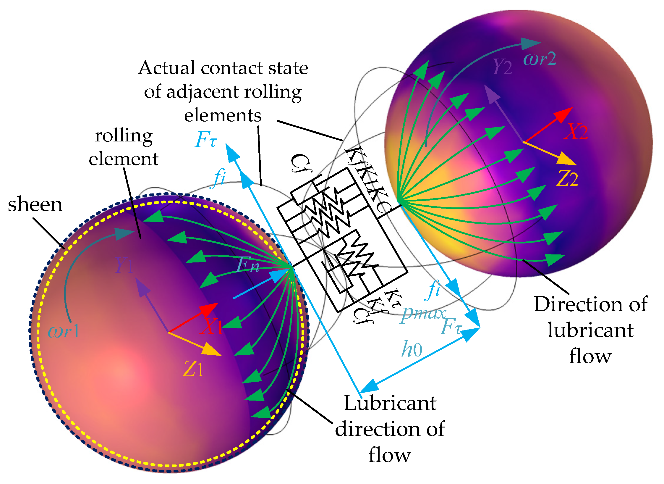
2. Modeling of Non-Smooth Bumper Vibration Considering Symmetry Collision of Neighboring Rolling Bodies with Oil Film Flow

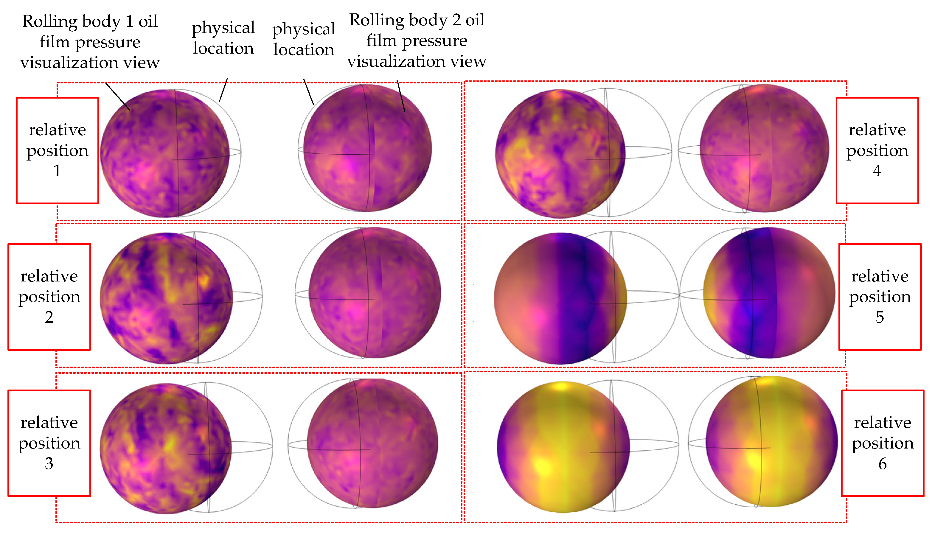
2.1. Rolling Body Oil Film Flow Characterization

A layer of lubricant is connected to each rolling element while the bearing is in use. When you do not think about how breaking the oil film due to moving body contact can cause wear, you should know that the two lubricants are always crashing into each other, so the thickness of the film cannot change. At this point, using the Navier–Stokes (N-S) equation, we can find the lubricant’s circular instantaneous velocity and axial instantaneous velocity, as well as their partial differential relationship.

$$\left\{\begin{array}{l}\frac{\partial p}{\partial x}=\eta \frac{{\partial }^{2}u}{\partial y^2}\\ \frac{\partial p}{\partial z}=\eta \frac{{\partial }^{2}w}{\partial y^2}\\ \frac{\partial u}{\partial x}+\frac{\partial v}{\partial y}+\frac{\partial w}{\partial z}=0\end{array}\right.$$

(1)

where η denotes the lubricant viscosity between neighboring rolling bodies and p denotes the oil film pressure between them.

Equation (1) can be solved quadratically along the other radial direction y of the bearing to obtain a mathematical model of the circular instantaneous velocity and the axial instantaneous velocity

$$\left\{\begin{array}{l}u=\frac{1}{\eta }\frac{\partial p}{\partial x}{{\displaystyle \int }}_0^{y}ydy+\frac{h\left[(u_2-u_1)-\frac{1}{\eta }\frac{\partial p}{\partial x}{{\displaystyle \int }}_0^{h}ydy\right]}{{\eta }^2}{{\displaystyle \int }}_0^{y}1dy+u_1\\ w=\frac{1}{\eta }\frac{\partial p}{\partial z}{{\displaystyle \int }}_0^{y}ydy+\frac{h\left[(w_2-w_1)-\frac{1}{\eta }\frac{\partial p}{\partial x}{{\displaystyle \int }}_0^{h}ydy\right]}{{\eta }^2}{{\displaystyle \int }}_0^{y}1dy+w_1\end{array}\right.$$

(2)

From Equations (1) and (2), the instantaneous velocity of the lubricant in the bearing and radial direction v is

$$\left\{\begin{array}{l}{{\displaystyle \int }}_0^h\frac{\partial u}{\partial x}dy+{{\displaystyle \int }}_0^h\frac{\partial v}{\partial y}dy+{{\displaystyle \int }}_0^h\frac{\partial w}{\partial z}dy=0\\ \nu =-\frac{\partial }{\partial x}{{\displaystyle \int }}_0^{y}udy-\frac{\partial }{\partial z}{{\displaystyle \int }}_0^{y}wdy\end{array}\right.$$

(3)

To obtain the greatest thickness of the lubricant oil film on the rolling body surface for h, use Equations (1)–(3) together. This will give you the oil volume per unit time for the bearing’s circumferential and axial oil:

$$\left\{\begin{array}{l}{m}_x=-\frac{\rho }{12\eta }{h}^3\frac{\partial p}{\partial x}+h\rho (\frac{u_1+u_2}{2})\\ m_z=-\frac{\rho }{12\eta }{h}^3\frac{\partial p}{\partial z}+h\rho (\frac{w_1+w_2}{2})\end{array}\right.$$

(4)

Format: $h(u,w)=h_0+\frac{u^2}{2R_u}+\frac{w^2}{2R_w}+\delta (u,w)$, $\rho ={\rho }_0(1+\frac{C_{1}p}{1+C_{2}p})$.

In order to visualize and analyze the dynamic process of oil flow generated by the oil film with the change of motion between adjacent rolling bodies, Equations (2)–(4) are dimensionless in this section.

$$\left\{\begin{array}{l}U=\frac{a{p}_h}{{\eta }_0{u}_e}\frac{H^2}{2\overline{\eta }}\frac{\partial P}{\partial X}\left(Y^2-Y\right)+\left(1-Y\right)U_1+U_2\\ W=U_1+\frac{a{p}_h}{{\eta }_0{u}_e}\frac{H^2}{2\overline{\eta }}\frac{\partial P}{\partial X}(Y^2-Y)\\ V=-H\left(\frac{\partial }{\partial X}{{\displaystyle \int }}_0^{Y}UdY+\frac{\partial }{k\partial Y}{{\displaystyle \int }}_0^{Y}WdY\right)\end{array}\right.$$

(5)

$$\left\{\begin{array}{l}{M}_x=-\frac{a{H}^3{p}_h}{12{\eta }_0}\frac{\overline{\rho }}{\overline{\eta }}\frac{\partial P}{\partial X}+\frac{H{u}_e}{2}\overline{\rho }(U_1+U_2)\\ M_z=-\frac{a^2{H}^3{p}_h}{12b{\eta }_0}\frac{\overline{\rho }}{\overline{\eta }}\frac{\partial P}{\partial X}+\frac{H{u}_e}{2}\overline{\rho }(U_1+U_2)\end{array}\right.$$

(6)

Format: $\overline{\eta }=exp\left\{(\ln {\eta }_0+9.67)\left[-1+{(1+5.1\times {10}^{-9}{p}_{h}P)}^{z_1}\right]\right\}$, $\overline{\rho }=1+\frac{C_1{p}_{h}P}{1+C_2{p}_{h}P}$.

Oil film on the moving body should keep adding oil so that it does not run out when it moves and hits things. This makes sure that elastic fluid stays on the moving body. We made a model that does not rely on size using the simple Reynolds equation to show how the oil film moves on top of the rolling parts of nearby cage-less ball bearings that have a useful slot:

$$\begin{array}{l}\frac{\partial }{\partial X}\left(\frac{a}{12u_e}\frac{p_h}{{\eta }_0}\frac{(1+\frac{C_1{p}_{h}P}{1+C_2{p}_{h}P})(H_0+\frac{a{X}^2}{2R_x}+\frac{k{Z}^2}{2a{R}_y}+V(X,Y))}{exp\left\{(\ln {\eta }_0+9.67)\left[-1+{(1+5.1\times {10}^{-9}{p}_{h}P)}^{z_1}\right]\right\}}\frac{\partial P}{\partial X}\right)\\ +\frac{\partial }{\partial Z}\left(\frac{a^3}{12b^2{u}_e}\frac{p_h}{{\eta }_0}\frac{(1+\frac{C_1{p}_{h}P}{1+C_2{p}_{h}P})(H_0+\frac{a{X}^2}{2R_x}+\frac{k{Z}^2}{2a{R}_y}+V(X,Y))}{exp\left\{(\ln {\eta }_0+9.67)\left[-1+{(1+5.1\times {10}^{-9}{p}_{h}P)}^{z_1}\right]\right\}}\frac{\partial P}{\partial Z}\right)\\ =\frac{\partial \left(1+\frac{C_1{p}_{h}P}{1+C_2{p}_{h}P}\right)\left(H_0+\frac{a{X}^2}{2R_x}+\frac{k{Z}^2}{2a{R}_y}+V\left(X,Y\right)\right)}{\partial X}\end{array}$$

(7)

The dynamics dimensionless model accurately predicts how the oil film volume changes along with its thickness, density, and viscosity when the cage-free ball bearings next to it are running. The model is solved in real time using Comsol 6.2 software to see how the oil film pressure changes so that the dynamic properties of the oil volume in the contact of the next rolling bodies can be studied.

We bring in a three-dimensional model of a local functional-slot cage-less ball bearing and set the rolling body dynamics solution formula to Equation (7). We then enter the calculation time, starting step, and calculation error for the exercise.

Table 1. Lubricating oil parameters of ball bearings without cages in local functional slots.

Parameters	Numerical Value
Rolling body 1 modulus of elasticity E1/GPa	207
Rolling body 2 modulus of elasticity E2/GPa	207
Initial lubricant viscosity η0/Pa·s	0.050
Lubricant viscous pressure coefficient α/m2/N	1.85 × 10−8
Poisson’s ratio for rolling stock υ1	0.29
Initial lubricant density ρ0/kg/m3	992

shows the lubricant characteristics. The load is a joint load with a radial load of 2000 N and an axial load of 200 N. The speed of the bearing is set to 10,000 r/min.

After the simulation, the Comsol software tracked the movement of two adjacent rolling bodies from contact to separation and recorded the real-time distribution and change of oil film pressure. The color change from purple to yellow shows that the oil film pressure gradually decreases; that is, purple means there is more oil in the film, and yellow means there is less oil in the film. This is shown in Figure 1.

Figure 1 shows that from relative position 1 to relative position 4, the two moving bodies are getting closer, but they are not touching or colliding. Position 5 shows the oil film pressure when the two rolling bodies hit each other, and position 6 shows the oil film pressure when the two rolling bodies are no longer touching each other. When the two rolling bodies are not touching, the oil film that surrounds them is not evenly distributed. The faster the spinning speed, the less even the oil film pressure is, and the fact that the film’s thickness is not consistent is a very bad thing. When two moving bodies hit each other, the inertia of the contact point pulls the center of the oil film quickly to the middle of the situation. This is especially true near the side contact point, where the oil film pressure rises right away and the film gets thicker. As soon as the two rolling bodies stopped touching each other, the oil film quickly moved from the middle to the two ends of the region to concentrate. This happened because of the siphoning effect. When the rolling bodies started rotating normally again, the oil film became uneven again. If you look at Figure 1, you can see that the oil film flow state will always bring the rolling bodies into touch with each other when things are not smooth. This causes the running instability of the bearing.

2.2. Modeling of Non-Smooth Vibrations of Adjacent Rolling Bodies

Combining the study of the moving parts of the contact oil, the clash between two rolling bodies next to each other is mathematically represented as a touching vibration with many degrees of freedom. Figure 2 shows the contact model that was made based on how the oil film flow changes between adjacent rolling bodies in the previous part.

Figure 2 shows that when two moving bodies next to each other crash into each other, the stiffness of the oil film changes, which in turn changes how well the lubricant works. When the results of the oil film pressure study are added to the mathematical model for a normal contact between two rolling bodies that are adjacent to each other,

$$\left\{\begin{array}{l}{K}_v={\left(\frac{1}{K_L}+\frac{1}{K_C}\right)}^{-1}+K_f\\ C_v=C_f\end{array}\right.$$

(8)

where K_L indicates the normal contact stiffness of the oil film; K_v indicates the equivalent lubrication stiffness of the lubricant when the neighboring rolling bodies collide; C_v indicates the equivalent lubrication damping of the lubricant when the neighboring rolling bodies collide; K_f indicates the stiffness of the oil film on one side of the rotational direction of the neighboring rolling bodies when they are in contact; K_C indicates the Hertzian contact stiffness; and C_f indicates the Hertzian contact damping.

The mathematical model of the motion state after the collision of adjacent rolling bodies can be calculated from Equations (7) and (8):

$$m\frac{{\mathrm{d}}^2\delta }{\mathrm{d}{t}^2}=K_v\delta +C_v\stackrel{•}{\delta }=-{\left(\frac{8}{9}\frac{{\pi }^2{J}_1{\kappa }^2{E_1}^2}{{J_2}^3{\displaystyle \sum \rho }}\right)}^{1/2}{\delta }^{3/2}$$

(9)

where κ denotes the contact ellipticity when adjacent rolling bodies collide, J₁ denotes the first type of elliptic integral, $J_1={{\displaystyle {\int }_0^{\pi /2}\left[1-\left(1-\frac{1}{{\kappa }^2}\right){\sin }^2\theta \right]}}^{-1/2}\mathrm{d}\theta$, and J₂ denotes the first class of elliptic integrals, $J_2={{\displaystyle {\int }_0^{\pi /2}\left[1-\left(1-\frac{1}{{\kappa }^2}\right){\sin }^2\theta \right]}}^{1/2}\mathrm{d}\theta$.

The quick acceleration of the rotor will cause nearby rolling bodies to fall into the inner ring. This will cause the relative speed between the two to instantly rise, putting them into the elastic compression stage. When the normal relative speed of the two rolling bodies is slowed down to zero and continues to go down, the two contact forms will enter the plastic deformation stage. The literature review tells us the key collision force of rolling bodies next to each other in this state:

$$F_{\sigma }=\frac{4}{3}{E}_0^{\prime }{{\displaystyle r}}^{3/4}{\left(\frac{3\mathsf{\pi }\vartheta \sigma }{4E_0^{\prime }}\right)}^{3/2}$$

(10)

where r denotes the radius of the rolling element; ϑ denotes the compressive deformation of the bearing steel material; σ denotes the yield stress of the bearing steel material; and E’₀ is related to the Young’s modulus and Poisson’s ratio of the bearing steel.

The mathematical model of motion in the collision phase of adjacent rolling bodies can be derived from Equations (9) and (10):

$$m\frac{{\mathrm{d}}^2\delta }{\mathrm{d}{t}^2}=-\left(\frac{2\pi J_1}{J_2{\displaystyle \sum \rho }}\sigma \delta \right)+\frac{8\sqrt{2}}{3}\mathsf{\pi }\frac{\kappa {J_1}^{5/2}{J_2}^{1/2}}{({\displaystyle \sum \rho {)}^{5/2}{E_0}^{\prime 3}}}{\sigma }^4{\delta }^{-1/2}-4\mathsf{\pi }\frac{{\kappa }_1{J_1}^2\sigma }{{\left({\displaystyle \sum \rho }\right)}^2{E_0}^{\prime 2}}$$

(11)

From Equation (11), the mathematical model of motion can be further obtained when adjacent rolling bodies enter the elastic–plastic recovery stage (the normal relative velocity of the two rolling bodies starts from 0 and gradually becomes larger) after the collision:

$$m\frac{{\mathrm{d}}^{2}t}{\mathrm{d}{t}^2}=-{\left(\frac{8}{9}\frac{{\mathsf{\pi }}^2{J}_1{E_0}^{\prime 2}}{{J_1}^3{\displaystyle \sum \rho }}\right)}^{1/2}{\left(\delta -{\delta }_{\sigma }\right)}^{3/2}$$

(12)

The oil film’s normal contact stiffness K_L in Equation (8) is calculated by taking partial derivatives of δ based on the mathematical models of collision and recovery phases of adjacent rolling bodies established in Equations (11) and (12):

$$K_L=\frac{3}{2}\left(\frac{2}{9}\frac{{\mathsf{\pi }}^2({{\displaystyle {\int }_0^{\pi /2}\left[1-\left(1-\frac{1}{{\kappa }^2}\right){\sin }^2\theta \right]}}^{-1/2}\mathrm{d}\theta ){\kappa }^2{E}^{\prime 2}}{{({{\displaystyle {\int }_0^{\pi /2}\left[1-\left(1-\frac{1}{{\kappa }^2}\right){\sin }^2\theta \right]}}^{1/2}\mathrm{d}\theta )}^3{\displaystyle \sum \rho }}\right){\delta }^{1/2}$$

(13)

The Hertzian contact stiffness between adjacent rolling elements can be found by combining Equations (5)–(7) and (13):

$$K_C=\frac{10}{1.8023}{E}^{\prime }\sum \rho {\left[\Delta V^{0.67}{E^{\prime }}^{0.53}{F}_n^{-1.067}(1-0.61e^{-0.73k})\right]}^{-1}$$

(14)

Substituting Equations (13) and (14) into Equation (8) can be performed to find the oil film stiffness and oil film damping on the side of the rotational direction when adjacent rolling bodies are in contact:

$$\left\{\begin{array}{l}{K}_f=\frac{4\eta \Delta v\sum \rho }{\frac{\frac{10h_c}{1.8023}{E}^{\prime }\sum \rho {\left[\Delta V^{0.67}{E^{\prime }}^{0.53}{F}_n^{-1.067}(1-0.61e^{-0.73k})\right]}^{-1}}{\frac{3}{2}\left[\frac{2}{9}\frac{{\pi }^2({{\displaystyle \int }}_0^{\pi /2}{\left[1-(1-\frac{1}{k^2}){\sin }^2\theta \right]}^{-1/2}d\theta )k^2{E^{\prime }}^2}{{({{\displaystyle \int }}_0^{\pi /2}{\left[1-(1-\frac{1}{k^2}){\sin }^2\theta \right]}^{1/2}d\theta )}^3\sum \rho }\right]{\delta }^{1/2}}+h_c}\\ C_f=\frac{6\pi \eta {(\sum \rho )}^{3/2}}{\sqrt{2}{h}_c^{3/2}}\end{array}\right.$$

(15)

The oil film flow of adjacent rolling bodies and Equation (15) show that when two adjacent rolling bodies hit each other quickly, if you do not take into account the rotation of the lubricant, the rolling bodies will have spherical flow on both sides, even though the rolling bodies are actually rotating. Because of inertia, when two rolling bodies collide, the lubricant builds up on one side, making it thicker than the other. This happens when the two bodies bump into each other in the direction of spin along the normal direction. But, it is not enough to just look at the normal direction to tell if the oil film rupture causes the adjacent rolling body contact form to change again. You also need to look at the tangential contact modeling study of the adjacent rolling body collision. Figure 2 shows that when two rolling bodies next to each other hit each other, the moving rolling bodies cause the lube oil film to move in a tangential direction. This lets us figure out the lube oil film shear force model:

$$\tau ={\displaystyle {\int }_0^t\frac{\tau }{\eta }}\mathrm{d}t$$

(16)

If two moving bodies next to each other crash because their rotational angular speeds are different, the oil film between them will cause friction in the tangential direction. This part sets up a mathematical model of how oil film’s rheological friction affects rolling things next to each other, using the rheological properties of non-Newtonian fluid lubrication:

$${\mu }_{\alpha }=3\eta \frac{U}{h_i}\frac{e^{\alpha p(\alpha p-1)}+1}{{\alpha }^2{p}^3}$$

(17)

where α indicates the viscosity coefficient of the oil film between neighboring rolling bodies after being pressurized.

From Figure 2, it can be seen that during adjacent rolling body collision, the oil film’s tangential stiffness then produces changes. Combined with the oil film pressure analysis results and the normal contact mathematical model established in this section, we can establish the adjacent rolling body collision tangential contact mathematical model:

$$F_{\tau }=(\frac{\tau }{\Delta {\omega }_{\gamma }rt}+K_f){\delta }^n+C_T\dot{\delta }$$

(18)

With the same trend of normal contact, the critical contact load Q_a of neighboring rolling bodies to keep the oil film unbroken is known from the literature review:

$$Q_a=\frac{EA{\sigma }_{\theta }(17e^{-2.84\lambda }+1.44\times {10}^{-4}{(\lambda -2)}^{1.1}{\left(4-\lambda \right)}^{7.8})}{4{\pi }^2}$$

(19)

where σ_θ denotes the slope of contact ellipse of neighboring rolling bodies and λ denotes the ratio of oil film thickness of neighboring rolling bodies.

The critical friction coefficient model for oil film rupture between adjacent rolling bodies can be established from Equations (17) and (19):

$$\begin{array}{l}{\mu }_s=3\eta \cdot \frac{U}{h_i}\cdot \frac{e^{\alpha p(\alpha p-1)}+1}{{\alpha }^2{p}^3}\cdot \frac{4{\pi }^2{F}_n-EA{\sigma }_{\theta }(17e^{-2.84\lambda }+1.44\times {10}^{-4}{(\lambda -2)}^{1.1}{(4-\lambda )}^{7.8})}{F_{n}4{\pi }^2}\\ +{\mu }_b\cdot \frac{EA{\sigma }_{\theta }(17e^{-2.84\lambda }+1.44\times {10}^{-4}{(\lambda -2)}^{1.1}{(4-\lambda )}^{7.8})}{F_{n}4{\pi }^2}\end{array}$$

(20)

where µ_b denotes the rolling element friction coefficient.

The oil film rupture critical friction force can be modeled from Equation (20):

$$\begin{array}{l}{f}_i=F_n(3\eta \cdot \frac{U}{h_i}\cdot \frac{e^{\alpha p(\alpha p-1)}+1}{{\alpha }^2{p}^3}\cdot \frac{4{\pi }^2{F}_n-EA{\sigma }_{\theta }(17e^{-2.84\lambda }+1.44\times {10}^{-4}{(\lambda -2)}^{1.1}{(4-\lambda )}^{7.8})}{F_{n}4{\pi }^2}\\ +{\mu }_b\cdot \frac{EA{\sigma }_{\theta }(17e^{-2.84\lambda }+1.44\times {10}^{-4}{(\lambda -2)}^{1.1}{(4-\lambda )}^{7.8})}{F_{n}4{\pi }^2}\end{array}$$

(21)

Because the adjacent rolling bodies are moving on the bearing raceways, the raceway geometry is circular, resulting in a certain angular deviation θ_n when the rolling bodies collide:

$${\theta }_n=\arctan \frac{F_{\sigma }}{F_n}$$

(22)

Mathematical equations based on Equations (15), (18), (21), and (22) are coupled to establish a non-smooth vibration model for adjacent rolling bodies:

$$F_i=\frac{\frac{4}{3}{E}_0^{\prime }{{\displaystyle r}}^{3/4}{\left(\frac{3\mathsf{\pi }\vartheta \sigma }{4E_0^{\prime }}\right)}^{3/2}}{\cos \arctan \frac{(\frac{\tau }{\Delta {\omega }_{r}rt}+K_f){\delta }^n+C_T\stackrel{•}{\delta }}{\frac{4}{3}{E}_0^{\prime }{{\displaystyle r}}^{3/4}{\left(\frac{3\pi \vartheta \sigma }{4E_0^{\prime }}\right)}^{3/2}}}+\frac{(\frac{\tau }{\Delta {\omega }_{r}rt}+K_f){\delta }^n+C_T\stackrel{•}{\delta }}{\sin \arctan \frac{(\frac{\tau }{\Delta {\omega }_{r}rt}+K_f){\delta }^n+C_T\stackrel{•}{\delta }}{\frac{4}{3}{E}_0^{\prime }{{\displaystyle r}}^{3/4}{\left(\frac{3\mathsf{\pi }\vartheta \sigma }{4E_0^{\prime }}\right)}^{3/2}}}$$

(23)

The F_i in Equation (23) is decomposed according to the three spatial planes of X − Y, Y − Z, and X − Z, which provides the basis for analyzing the rolling body displacement and angular attitude of local functional-slot cage-less ball bearings in the next section.

3. Dynamic Characterization of Rolling Bodies Considering Oil Film Flow

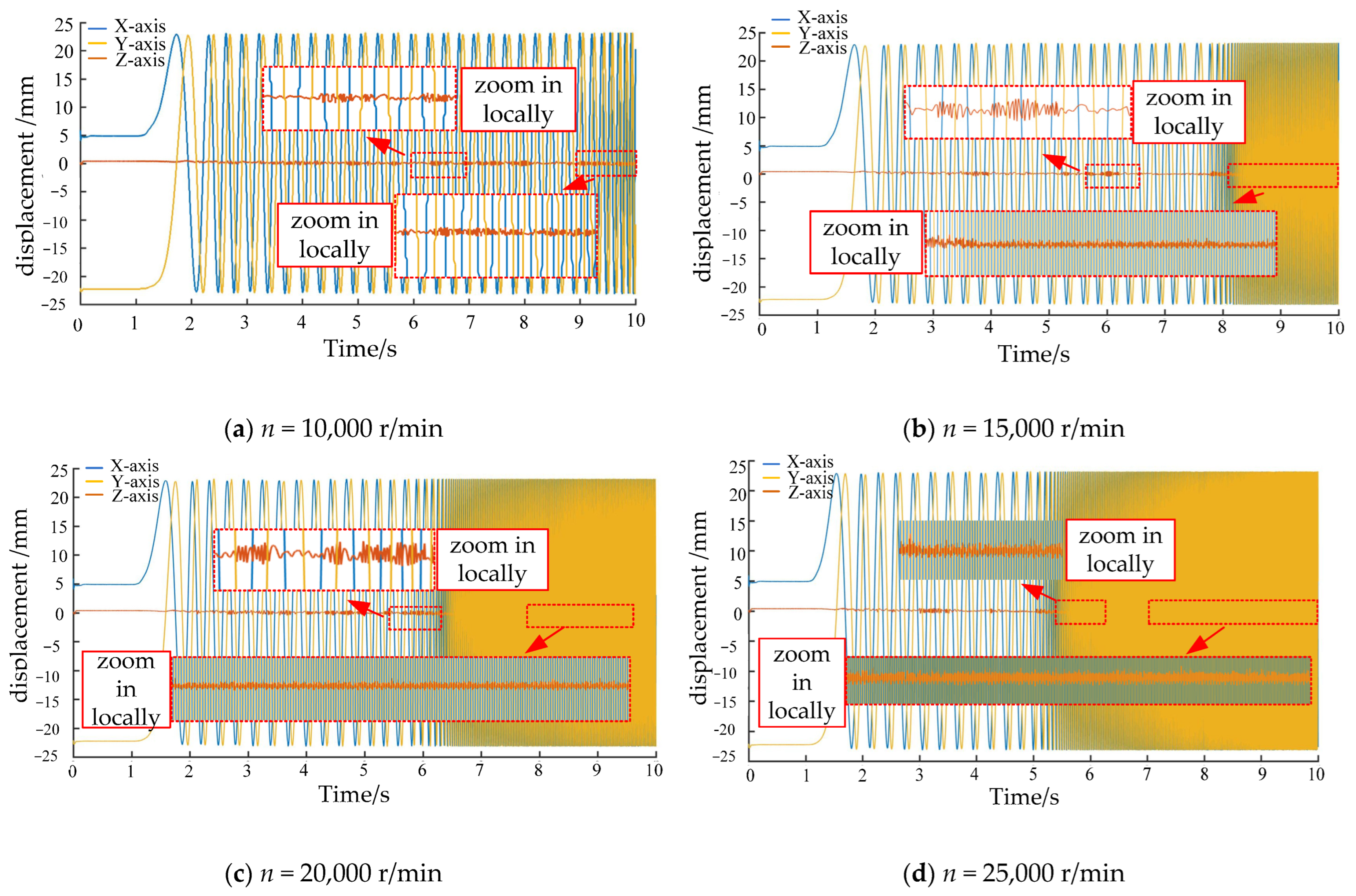
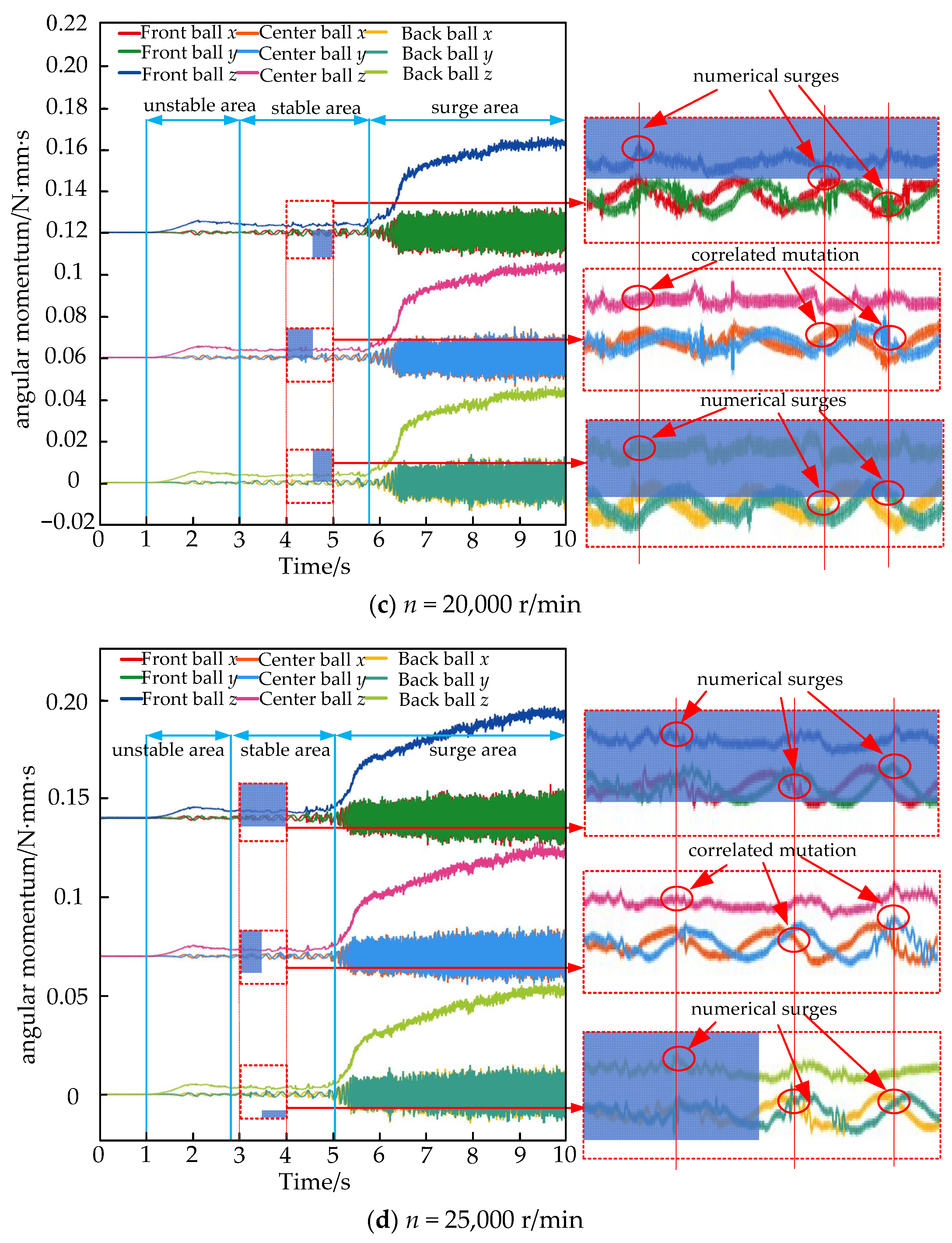
3.1. Rolling Body Displacement and Angular Attitude Analysis

This part uses the fourth-order and fifth-order Lunger–Kutta integration method with variable step size to figure out the rolling body’s displacement and angular momentum while taking into account the flow of the oil film and collisions that do not happen smoothly in a straight line. It also looks at how the rolling body’s overall collision shape changes after the local function slot is set up. After setting the rotor’s dropping speed to 10,000 r/min, 15,000 r/min, 20,000 r/min, and 25,000 r/min, centrifugal force will take over and make the rolling element less stable [32]. As a result, no working condition with a speed greater than 25,000 r/min was chosen. The load was set as a joint load, with 2000 N of radial load and 200 N of axial load. The rolling body’s motion was solved in three directions, as shown in Figure 3.

If the rotor falls and hits the inner ring, it moves with the rotation, and the rolling body moves with the rotation along with the inner ring. As we look more closely at Figure 3, we can see that the rolling body moves along the X-axis and Y-axis, following the law of periodic interval change. However, the curve at the farthest point in the negative direction of the Y-axis is not smooth, and there is an area with curving. This is because the bearing area has the lowest set of useful slots. This causes the rolling body’s rotational speed to first rise and then fall, which changes the rate of displacement. The movement change is slower at first and then faster when the rolling body passes the farthest point in the positive direction of the Y-axis. This is because the farthest point in the positive direction of the Y-axis is in the part of the bearing that is not carrying anything. As soon as the rolling part gets close to the highest point, gravity stops it from turning. Gravity will speed up its movement after the highest point, which will cause small but quick changes in the moving body’s position. The most obvious change in the z-axis displacement rate is when the rolling body goes through the functional slot. In the bearing contact angle, gravity and the structure of the functional slot work together to cause the z-direction displacement to happen at a very low value but a higher frequency. The rate of change in movement is much faster when the motion of the dropped rotor on the inner ring is stable. Looking at Figure 3a–d, we can see that as the falling rotor speed goes up, the time it takes for either rolling body to reach the stability stage in the X- and Y-axes directions goes down. Because the rate of change in displacement is less important, as the rolling body moves through the highest point of the functional slot and the non-bearing area, the faster the rotor drop speed. Instead, as the rotor drop speed goes up, the rate of change of the rolling element’s displacement in the Z-axis direction goes up. Shown in Figure 3 is the rolling body’s overall motion trend. To gain a better idea of how it affects other rolling bodies when it rotates, this section is further focused on solving the angular momentum changes along the X-axis, Y-axis, and Z-axis. This gives us three sets of angular momentum comparison plots for the rolling body, which are shown in Figure 4.

It is clear from Figure 4 that the rolling body will move in three different ways after the rotor falls and turns the inner ring of the bearing. These are the unsteady zone, the smooth zone, and the surge zone. The Z-direction (axial) angular displacement change of an unstable-zone rolling body is clear; the value goes up and then down. The X-direction and Y-direction (radial) angular displacement changes are smoother, though there are times when the rate changes from slow to fast. When the rolling body first starts to move, its rotation and rotational speed are slow because of the contact angle and the axial rotation tendency of the joint. But, as the speed goes up, the rotation and rotational movement gradually take over the rolling body movement. On a smooth surface, the rolling body’s angular momentum change is more stable in all three directions. However, there is a local value of the surge that happens because the rotor slips in the inner circle, which is caused by the rolling body’s unstable rotation. As the speed of the inner ring and rotor tends to stabilize, the rolling body’s angular displacement moves into the surge area. The axial angular displacement value surge is clear, and the radial angular displacement for speed change frequency surge is clear. This shows that the centrifugal force is controlling the rolling body’s movement at this point, causing the rolling body to move to the middle of the bearing and the contact angle of the bearing to become smaller. From Figure 4a–d, we can see that as the rotor’s falling speed goes up, the rolling body’s angular movement in the unstable zone does not last as long. Because the smooth zone does not last as long, it enters the surge zone more quickly. But, when the rolling element’s angular displacement in the axial direction enters the surge zone, the surge value goes up a lot. This means that the value of the bearing contact angle goes down a lot, which makes the operation of the bearing a lot less certain.

In Figure 4, the rolling body angular displacement of the smooth area over the same amount of time is shown on the right side of the local zoom map. It can be seen that when there is a sudden change in the angular displacement value of the middle ball, there must be one or even two balls with the same numerical magnitude and occurring simultaneously in the front and back balls.This shows that the value of the middle ball’s angular displacement is linked to the quick change, which means that the rolling bodies are colliding. The front ball, middle ball, and back ball all changing at the same time shows that the three rolling bodies collide, but this does not happen very often, as you can see from the zoomed-in picture on the right. In the next section, we will look at the collision forces in three directions of adjacent rolling bodies in order to gain a better idea of how many collisions there are and what kinds of collisions there are. After setting up the local function slots, we will then look at the overall collision form of the rolling bodies.

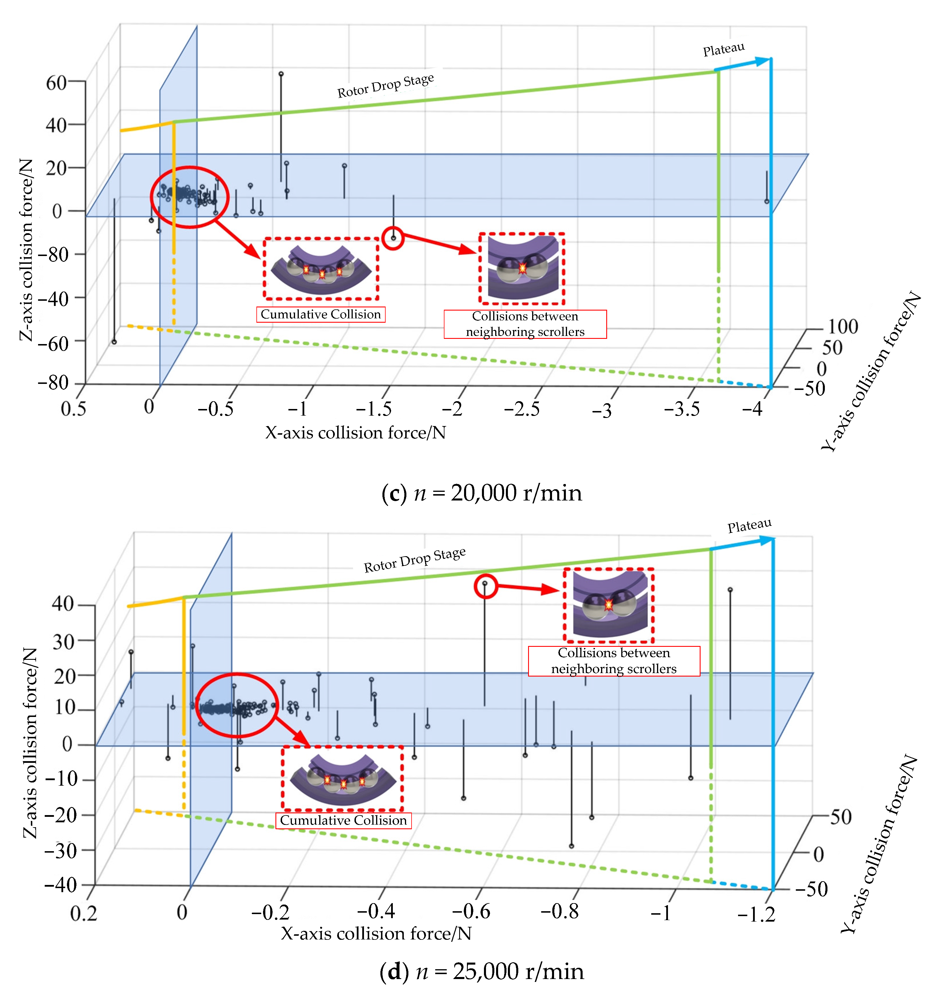
3.2. Rolling Body Overall Collision Form Analysis

By looking at the angular momentum of three rolling bodies in a row in the previous section, we saw that cumulative collisions and collisions of adjacent rolling bodies happen from time to time during the whole bearing operation. However, the angular momentum alone cannot tell us where these collisions happen or what their overall trend is. In this part, we use the standard multi-body dynamics solution process for cage-free ball bearings and the geometric data of the bearings (shown in

Table 2. Calculation parameters for collision forces of rolling bodies in three directions.

Parameters	Numerical Value
Poisson’s ratio for rolling stock/υ1	0.29
Number of scrollers/Z	14
Inside diameter d/mm	30
Outer diameter D/mm	62
Height B/mm	16
Rolling body radius r/mm	4.7625
Rolling body mass m/kg	0.01
Radial load Fr/N	2000
Axial load Fa/N	200
Rotation speed n/(r/min)	10,000/15,000/20,000/25,000
Poisson’s ratio for rolling stock µ1	0.29
Poisson’s ratio of inner and outer ring µ2	0.3
Localized functional slot Poisson’s ratio µ3	0.3
Initial lubricant density ρ0	992 kg/m3
Initial lubricant viscosity η0	0.050 Pa·s
Modulus of elasticity of a rolling body E	207 GPa
Modulus of elasticity of inner and outer ring E/Mpa	208,000
Lubricant viscous pressure coefficient α	1.85 × 10−8 m2/N

) to solve the collision forces of the rolling bodies in the X-, Y-, and Z-directions in a way that takes into account direction.

We use numbers to figure out the collision force between rolling bodies that are next to each other in three directions (X, Y, and Z) while the machine is moving and then de-time the data. This paper uses (0, 0, 0) as the center of the inner ring of the bearing because the impact force is a vector. The four quadrants that are made show the four regions of the bearing, with the load-bearing regions taking up two regions each. After the collision force data have been handled, a needle diagram like the one in Figure 5 is made.

By looking at Figure 5, we can see that when two rolling bodies next to each other fall during the pre-rotor stage, they will hit each other more than once. This will happen in the area where the load-bearing and non-load-bearing areas meet. This is because the rolling body is not rotating or rotating fast enough, which is the same as what the angular displacement study showed. When the bearing operation enters the stabilization period, neighboring rolling bodies still collide, but their number of collisions is much lower, and there is no continuous cumulative effect. This shows that the local function slot does what it was meant to do from the start and controls the rotation of the rolling body.

From Figure 5a–d, we can see that the maximum axial collision force rises as the speed of the rotor falls from 10,000 r/min to 25,000 r/min. However, the general collision form law of the rolling bodies next to each other stays the same. But, compared to the axial collision force at a falling speed of 20,000 rpm, the maximum value at 25,000 rpm is not very strong, and there are more collisions between rolling things that are close to each other. Adding the angular displacement analysis to the picture shows that this is because the bearing contact angle is getting smaller and closer and closer to the critical value that is caused by the bearing working in a way that causes irregular vibrations, which leads to a big rise. We need to look into the fractal motion of rolling bodies and the chaotic features of their impact in order to answer the question of whether there is a non-smooth connection between the non-smooth collision of rolling bodies and the uneven vibration of bearings.

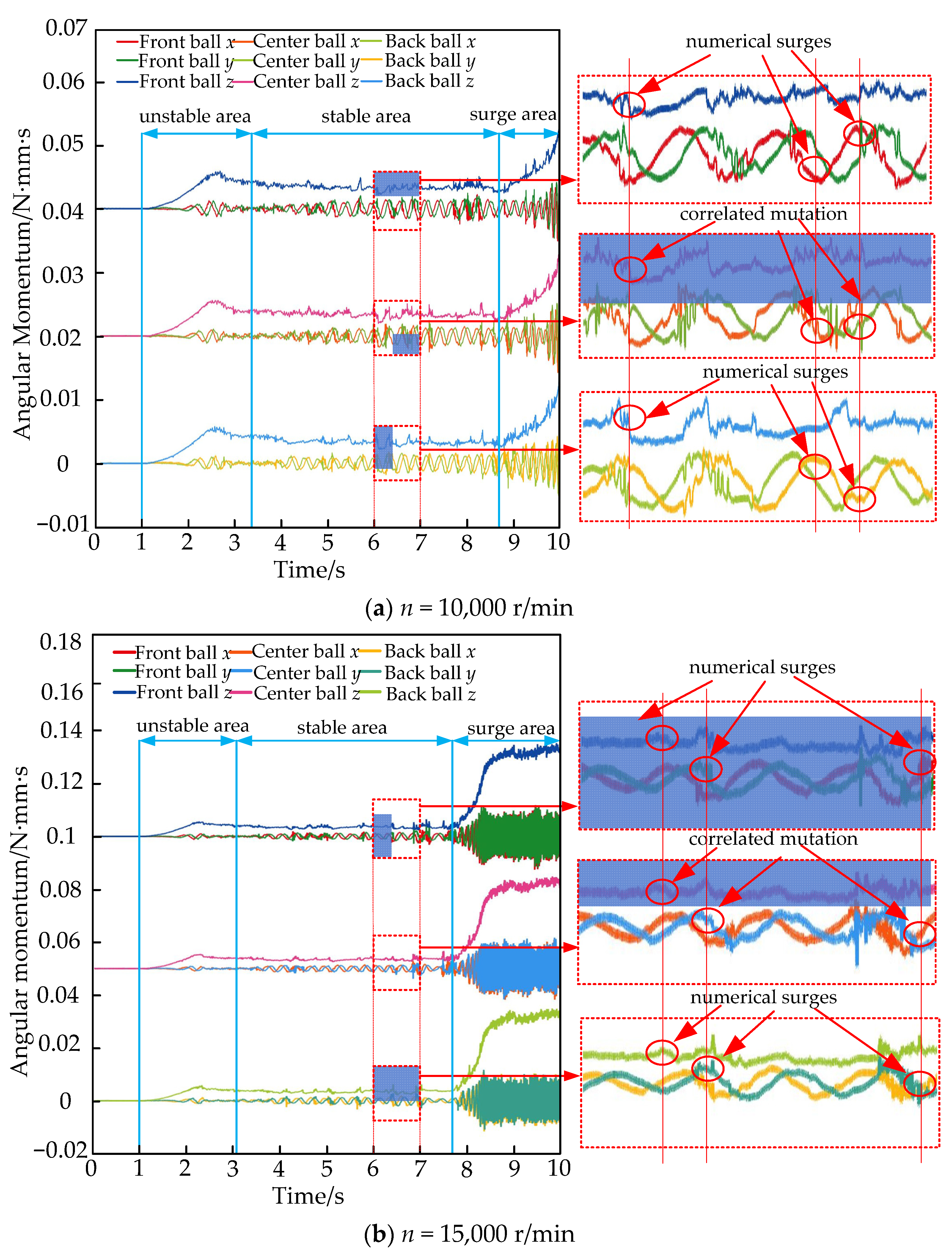
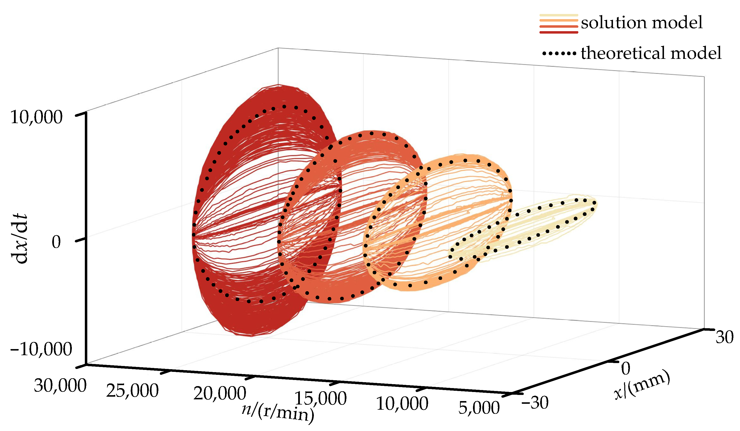
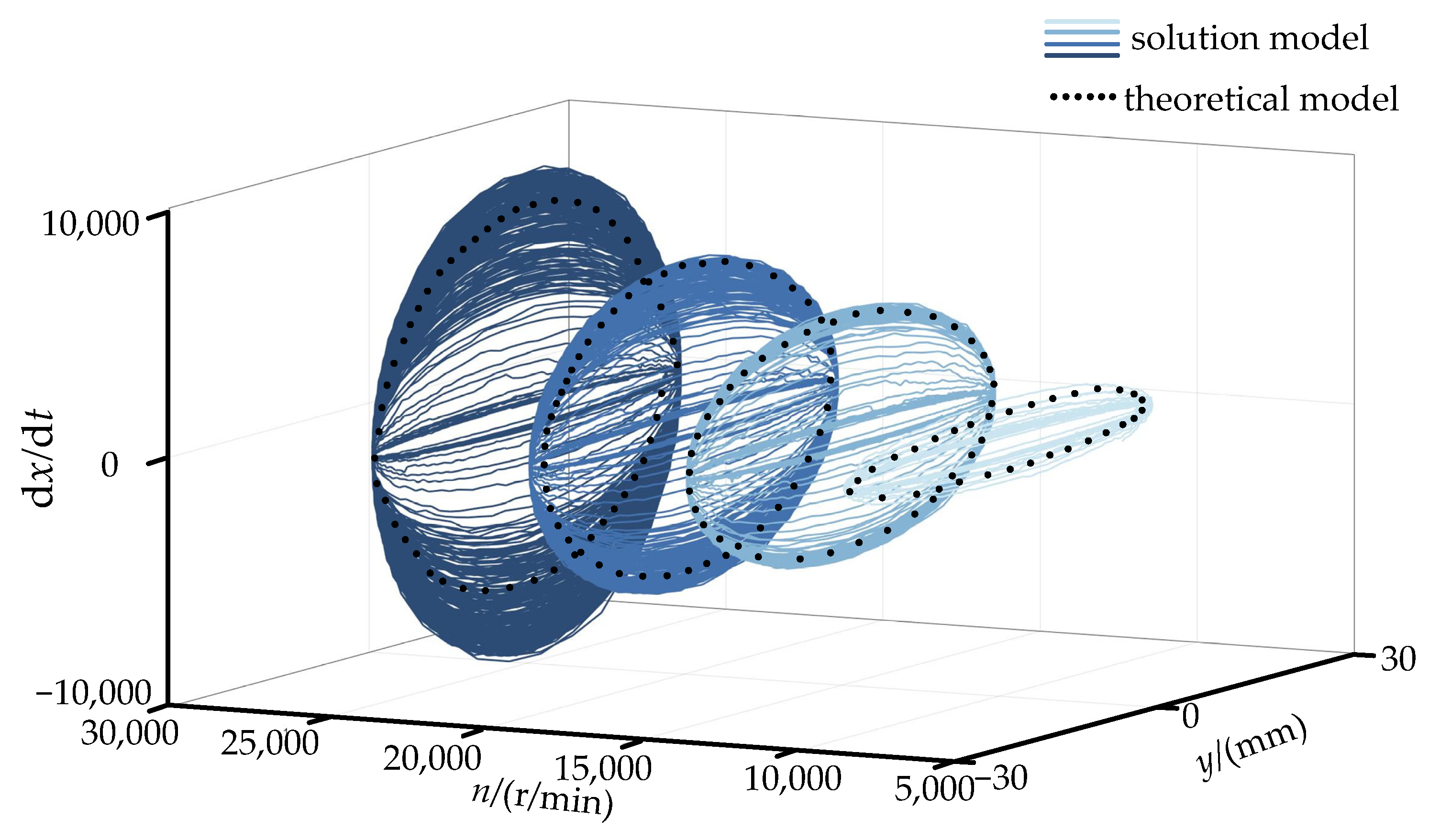
3.3. Chaotic Characterization of Rolling Body Motion

It is known that when rolling bodies collide, the motion becomes chaotic. In this section, we compare and analyze the phase diagrams of the system in the X-, Y-, and Z-directions at different speeds with a theoretical model of rolling body motion in its ideal state to look into the chaotic features that occur when two rolling bodies collide next to each other. Before obtaining the fractal comparison diagram of rolling body motion, the displacement and velocity data of bearing rolling bodies are solved directionally at four falling speeds of 10,000 r/min, 15,000 r/min, 20,000 r/min, and 25,000 r/min. The falling speed, displacement, and velocity data are then fitted into the system phase diagram using Matlab 2021b software. In Figure 6, you can see a comparison picture of the rolling body’s motion in the X-direction.

If you look closely at Figure 6, you can see that the rolling body’s motion in the X-direction is shown by a graph with many lobes, many levels, and a structure that is the same for each lobe and level. Using the three stages found by the rolling body angular momentum analysis, we can see that the rolling body’s motion in the X-direction has an infinite level of self-similar fractals in the unsteady zone, the stable zone, and the surge zone. This means that the rolling body’s motion in each cycle is not repeated during the whole mixing motion. The response form of the rolling element does not change when the rotor dropping speed is changed, and the fractal still has an endless number of levels of self-similarity. When looking at the geometric model of the bearing center diameter in the X-direction, it is found that the fractal is smaller at speeds of 15,000 r/min and 20,000 r/min. The fractal of the rolling body’s motion is also smaller at 10,000 r/min. However, when looking at the dynamic characteristics of the inner ring of the bearing under variable operating conditions, it can be seen that the inner ring of the bearing enters a stabilization period for a long time, which causes the rolling bodies to crash into each other over and over again. There are more collisions between adjacent rolling bodies than times. There are more collisions between rolling things that are close to each other. Figure 7 shows a fractal image of a rolling body moving in the Y-direction.

By looking at Figure 7, we can see that the rolling body has an infinite level of self-similarity structure in the Y-direction. This means that each cycle does not happen again, and it is moving in a chaotic way the whole time. The rolling body’s reaction form does not change when the rotor’s falling speed is changed, either. It is still a random motion with no pattern. The rolling body’s motion in the X-direction is more uniform, but the motion fractal in the Y-direction is more varied. This is because of the neighboring rolling body colliding and blocking the spin, as well as the local function of the slot structure working together.

We compared different speed conditions side by side and found that the solution model and the bearing center diameter in the Y-direction of the geometric model were still 15,000 r/min and 20,000 r/min, which means that the rolling body movement is more stable. A comparison of the fractal of a body rolling in the Z-direction is shown in Figure 8.

When you look at Figure 8, you can see that the rolling body’s movement fractal in the Z-direction (bearing axial) is more chaotic than in the X- and Y-directions (bearing radial). This is because the rolling body’s movement is always changing, and it has even been seen jumping back and forth along the Z-direction. The ideal state geometric theory model of the rolling body of the bearing in the Z-direction shows that the less quickly it rotates, the less fractal it is. However, in practice, bearings are usually used in pairs, which stops the contact angle from changing too much. This stops the rolling body from moving in a chaotic way in the Z-direction.

You can see from the above analysis that the motion fractal can only give you a qualitative picture of the rolling body’s chaotic motion when the rotational speed is changing. It cannot tell you how much the changing rotational speed affects its chaotic motion. This section chooses the Lyapuov index (later called the Li index) that was created by the famous Russian mathematician Li Yapuov to make it easier to combine relevant experiments and experiments on the local function slot without-cage ball bearing speed conditions for optimization. The Lyapuov index is used to measure the degree of chaos in the rolling body in the X-, Y-, and Z-directions of the motion data.

Since scholars started to learn about the Ly index, it has been used a lot in many areas of scientific study. Many changes have been made to the Li index by scholars from different countries to account for the differences in their study fields. The most important thing for increasing the accuracy of computations is to choose a Li index model that works well in their own fields. Because of this section, the study of the chaotic features of rolling body motion, and the creation of the multi-degree-of-freedom vibration model, it is clear that its motion is not smooth, and the dynamics model has a strong non-smooth feature. In this part, we will use the orthogonalization method to solve the Li index because Wolf and other researchers have made it better for systems that are not smooth. To begin, the non-smooth equations need to be changed in relation to the state vector (n × 1) so that they can be written as a function in terms of time. The equations that have been changed are then changed into the state vector (n × 1):

$$\left\{\begin{array}{c}x\\ {\psi }_t\end{array}\right\}=\left\{\begin{array}{c}f(x)\\ {\left.{\psi }_t\frac{\partial f_i}{\partial x_j}\right|}_{x_j=x_j(t)}\end{array}\right\}$$

(24)

where F (t) is denoted as the (n × n) Jacobi matrix.

After defining the initial values, the initial non-smooth equations are combined with Equation (24) to obtain the combined equations containing the initial values:

$$\left\{\begin{array}{c}{x}_{(0)}\\ {\psi }_{t(0)}\end{array}\right\}=\left\{\begin{array}{c}{x}_0\\ {[e_1^T(0) e_n^T(0)]}_{n\times n}\end{array}\right\}$$

(25)

Format: e₁(0) = (1, 0, …, 0), e₂(0) = (0, 1, 0, …, 0), …, e_n(0) = (0, 0, …, 1).

Substituting the initial value condition into Equation (24) for integration, a number of vectors are obtained, and then these vectors are processed using Schmidt’s renormalization method to create a new set of functions:

$$\left\{\begin{array}{l}{e}_1(\tau )=\frac{{\nu }_1(\tau )}{\left|\right|{\nu }_1(\tau )\left|\right|}\\ e_2(\tau )=\frac{{\nu }_2(\tau )-〈{\nu }_2(\tau ),e_1(\tau )〉e_1(\tau )}{‖{\nu }_2(\tau )-〈{\nu }_2(\tau ),e_1(\tau )〉e_1(\tau )‖}\\ \\ e_n(\tau )=\frac{{\nu }_n(\tau )-〈{\nu }_n(\tau ),e_1(\tau )〉e_1(\tau )- -〈{\nu }_n(\tau ),e_{n-1}(\tau )〉e_{n-1}(\tau )}{\left|\right|v_n(\tau )-〈v_n(\tau ),e_1(\tau )〉e_1(\tau )- -〈v_n(\tau ),e_{n-1}(\tau )〉e_{n-1}(\tau )\left|\right|}\end{array}\right.$$

(26)

After extracting the denominator in Equation (26) (denoted as p_i(m)), the orthogonalized Li exponential mathematical model is obtained by correcting the conventional expression after s integrals have been obtained:

$${\lambda }_i\approx \frac{{\displaystyle \sum _{m=1}^s{\log }_2{p}_i(m)}}{s\tau }(i=1,\dots ,n)$$

(27)

To make it easier to measure the level of chaos for side-by-side comparison, the mathematical model of the rolling body dynamics of the self-discrete system is run at four different rotational speeds of 10,000 r/min, 15,000 r/min, 20,000 r/min, and 25,000 r/min in the X-, Y-, and Z-directions. The orthogonalized Li exponential model solving process is used to obtain the results, which are then imported into Matlab. The data are then taken out in Matlab, and

Table 3. Maximum Lyapunov exponent of chaotic motion of rolling bodies.

Orientations	10,000 r/min	15,000 r/min	20,000 r/min	25,000 r/min
x-directional	4.5933	4.2011	3.9126	3.9158
y-directional	4.6431	4.2613	3.9350	3.9094
z-directional	7.6814	7.9442	7.9972	8.6271

shows the maximum Li Yapunov exponent data table of the random motion of the rolling body.

With the exception of 25,000 r/min, Table 3 shows that the rolling body’s motion is much less smooth in the z-direction than in the x- and y-directions. The values in the y-direction are slightly higher than those in the x-direction. Using the rolling body and inner ring motion attitude as a whole, it is clear that when the rotor falls at a speed of 25,000 r/min, the centrifugal force on the rolling body’s motion increases. This is because the centrifugal force value increases, which backs up the analysis of the angular momentum of the three rolling bodies in a row. In the x-direction, centrifugal force has a smaller effect on the rolling body’s motion than in the y-direction. In fact, the value of the working state at 25,000 r/min is a little higher than that at 20,000 r/min. This event backs up the study’s claim that the localized functional slot can control the moving body’s speed.

4. Experimental Study of Vibration Response of Adjacent Rolling Bodies

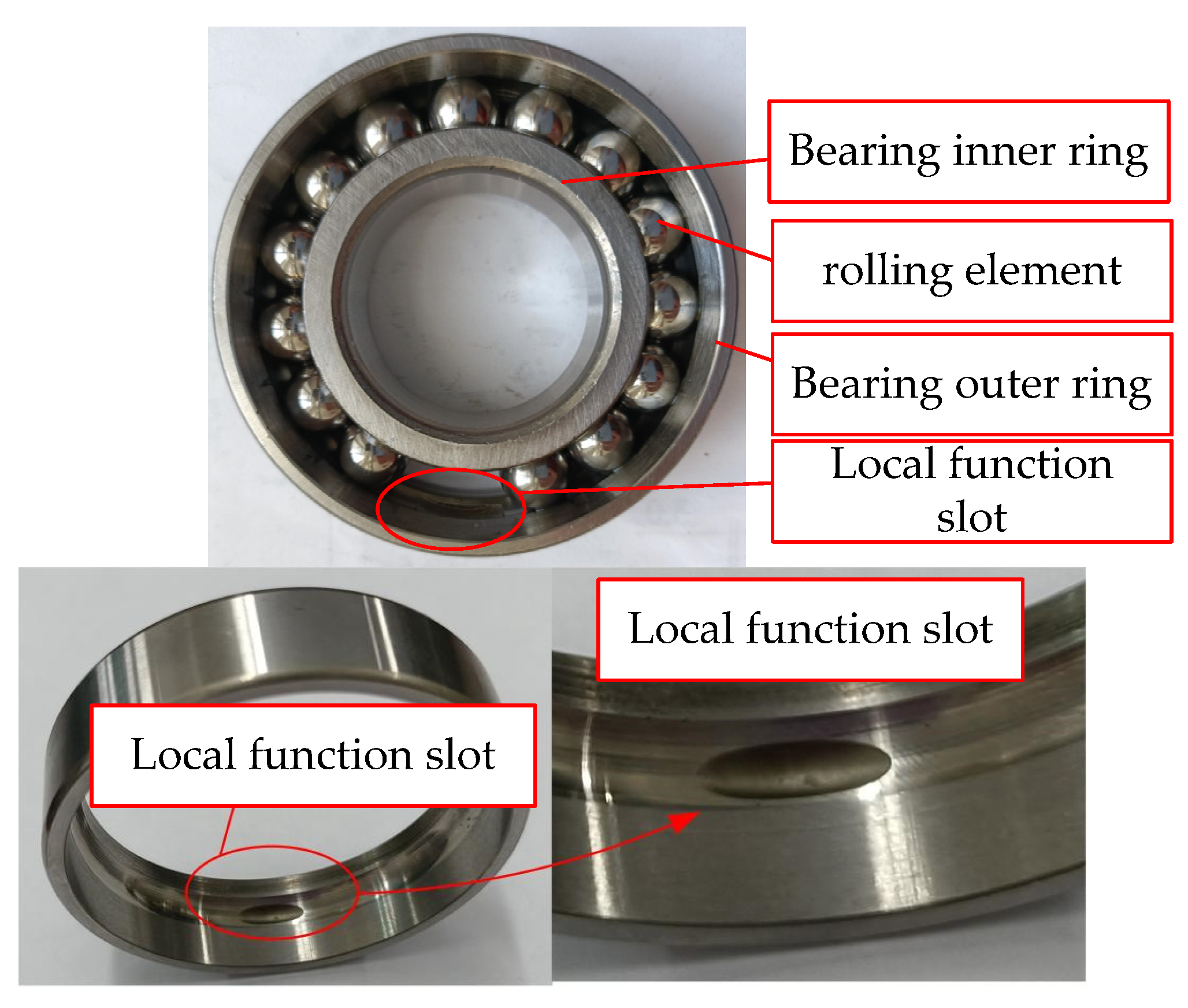
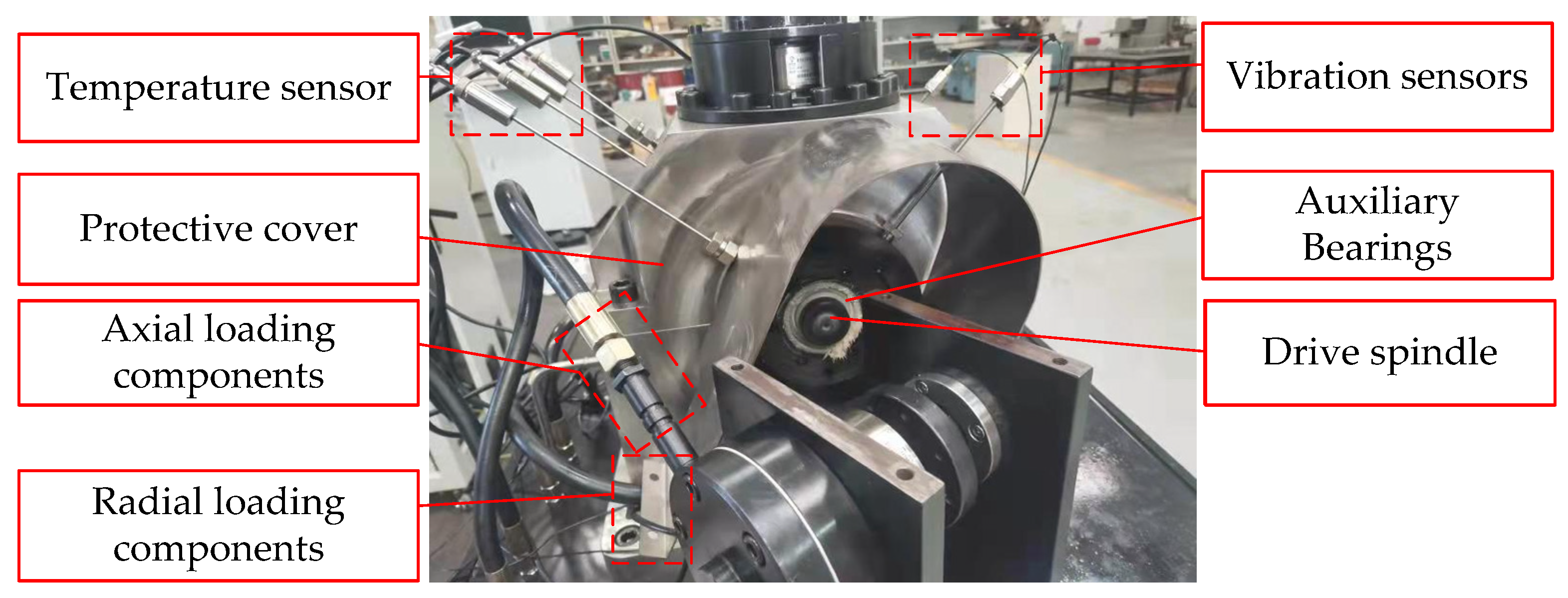
4.1. Vibration Response Experimental Program Design

This section will use experimental research to look into the uneven shaking of the bearing caused by rolling body collision and other factors. The goal is to learn more about the non-smooth behavior of local functional-slot non-cage ball bearing rolling body collision and how it affects the bearing’s operation.

In this part, EDM is used to make experimental bearings with functional slots in specific places, as shown in

Table 4. Partial functional slot test bearing parameters.

Expressed Symbol	Designation	Numerical Value	Unit
Z	Number of rolling bodies	14	number
Wu	Local function slot width	3.5	mm
Lu	Local function slot length	11.5	mm
Hu	Local function slot depth	1	mm
Dm	Pitch circle diameter	46.005	mm
Di	Inner ring slot bottom diameter	36.48	mm
ri	Radius of curvature of inner ring slot bottom	4.905	mm
Dw	Rolling body diameter	9.525	mm
Do	Outer ring slot bottom diameter	55.53	mm
ro	Radius of curvature of outer ring slot bottom	4.953	mm

. This is performed to reduce vibrations other than the roughness that happens when rolling elements crash into each other.

The experimental samples were prepared according to the parameters shown in Table 4, and the experimental samples of irregular vibration of bearings shown in Figure 9 were obtained.

In this part, we set the following requirements for the testing conditions of bearing irregular vibration. It can go from 1800 r/min to 8000 r/min, and the radial load Fr can be anywhere from 500 N to 2000 N. The axial load Fa can be anywhere from 300 N to 500 N. In order to measure the vibration signs of the local functional-slot cage-less ball bearing, the T10-60 model bearing experimental machine (Luoyang Research Institute, Luoyang, China)is chosen, as seen in Figure 10. There is a flexible connection between the main shaft of the T10-60 experimental machine and the high-speed electric spindle. The high-speed electric spindle can go as fast as 24,000 r/min. There is a flexible connection between the main shaft of the T10-60 experimental machine and the high-speed electric spindle. The high-speed electric spindle can go as fast as 24,000 r/min. There are three sets of bearings on the main shaft: the experimental bearings for uneven vibration and four deep-slot ball bearings. The experimental bearings are installed in the top set of bearings, and the deep-slot ball bearings are installed in the other two sets. To measure the radial load of the T10-60 experimental machine, the load is put on the bearing bush in the middle position and then sent to the experimental uneven vibration bearing. This is performed using the two deep-slot ball bearings.

With the above tools and the experimental bearing ready for irregular vibration tests, this section sets the experimental speed to 3000 r/min and places vibration sensors near the end of the experimental bearing. This makes it easier to compare the effects of different rotational speeds on the irregular vibration value and lessens the effect of extra vibration caused by the high speed.

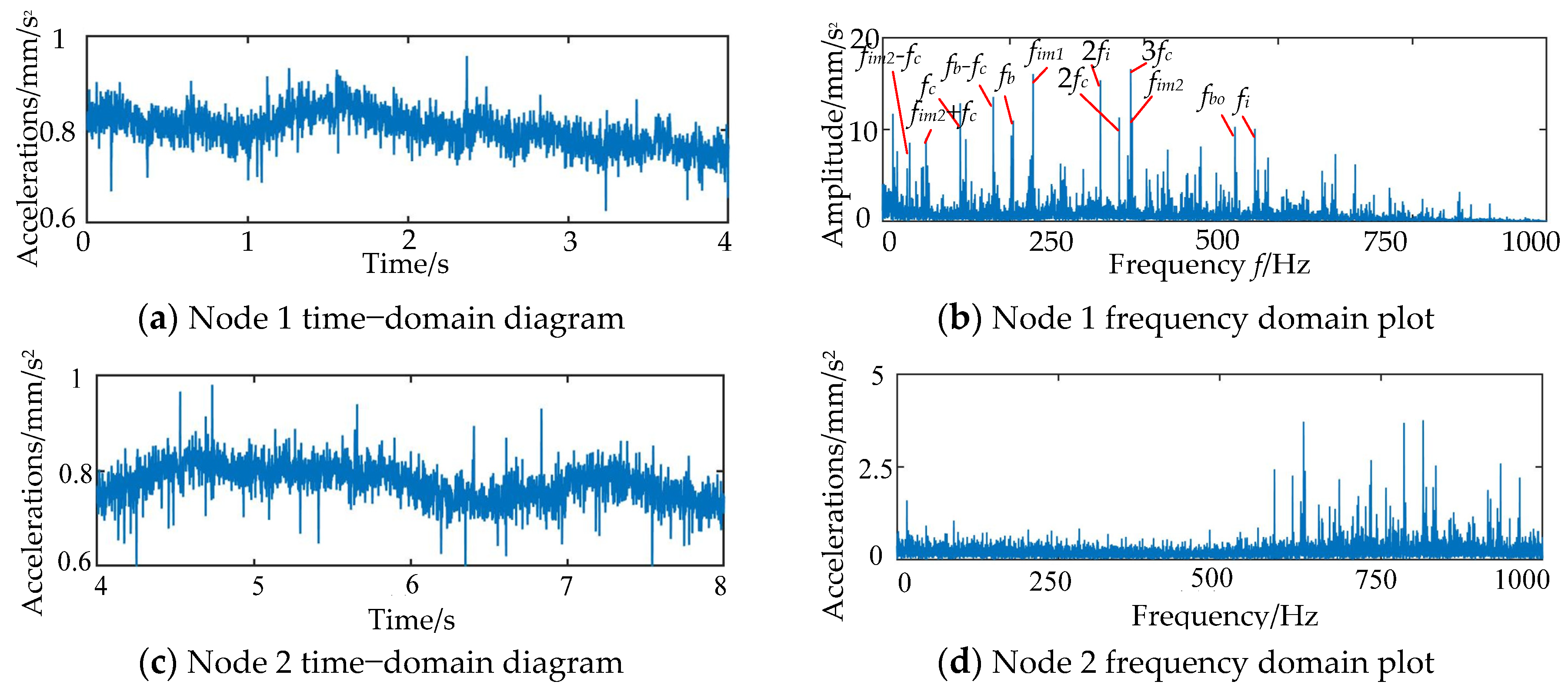
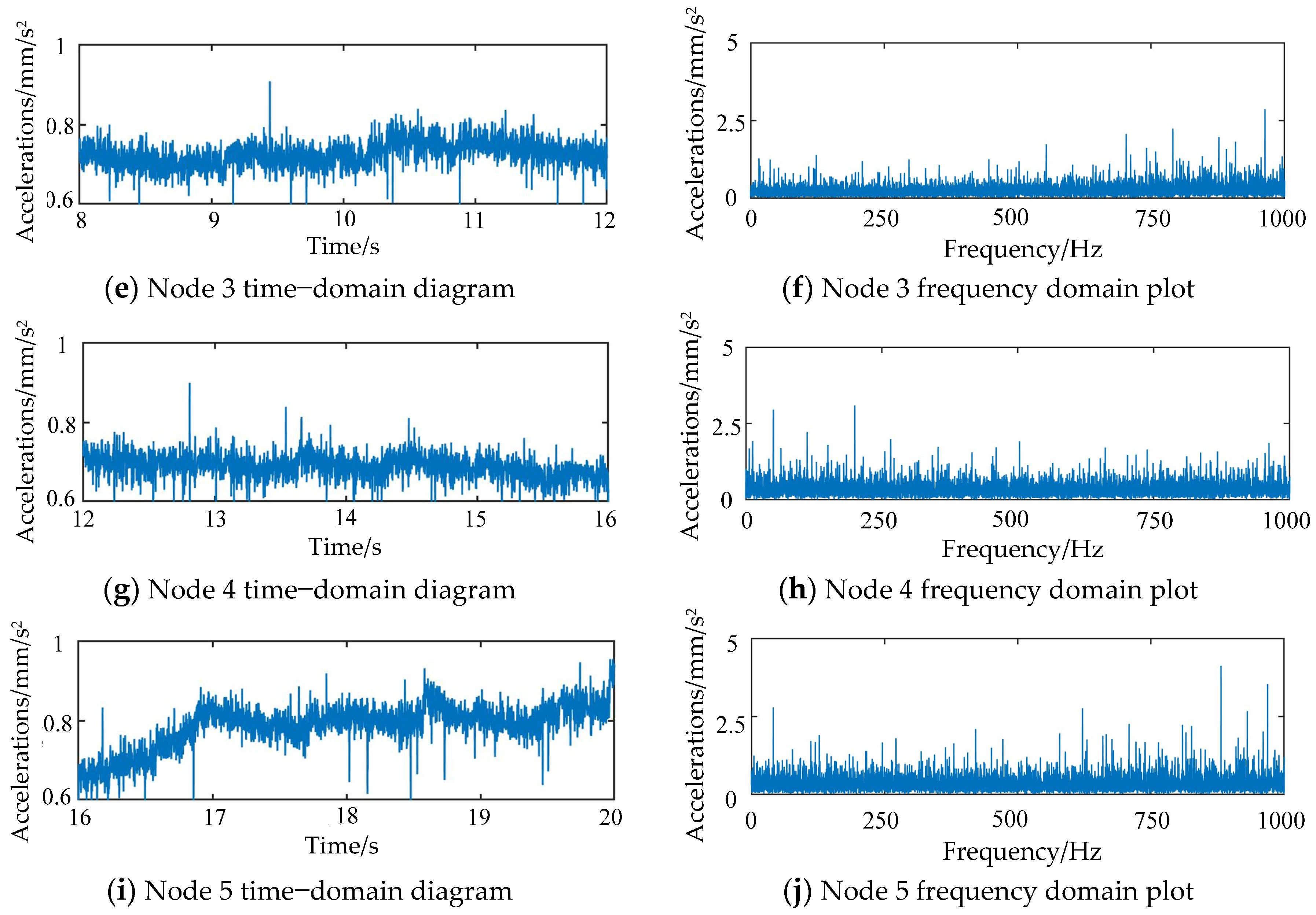
4.2. Analysis of Non-Smooth Vibration Response to Collision of Neighboring Rolling Bodies

When the machine is actually working, the speed and vibration properties of the local function-slot without-cage ball bearing are important. Based on the collision force, rolling body displacement, and angular attitude analysis, it can be seen that when two rolling bodies collide next to each other, the impact signal creates a vibration signal with a low frequency and a high frequency. To get rid of these signals, this paper uses wavelet analysis and the soft threshold method of vibration signal denoising to try to avoid adding more vibration to the data collection process. The noise is removed from the data, and then the frequency is shifted. This gives us the uneven vibration signals of a 3000 r/min non-cage ball bearing with a local functional slot.

You can see from Figure 11 that the local function-slot without-cage ball bearing’s uneven vibration time–domain signal in node 1 shows an acceleration from high to low trend. Nodes 2 through 4 show a smoother acceleration trend, and node 5 shows a rapid acceleration trend. The above trend matches the inner ring and rolling body motion attitude in the trend, which shows that the theoretical analysis is correct. At the same time, it is discovered that the acceleration surge phenomenon is stronger in the stage from node 2 to node 4, which means that there are more collisions between rolling bodies in this stage.

First, the time–domain signals are analyzed, and then the frequency domain signals are put together. The low-frequency signals are then found. We looked at the dynamic characteristics of the cage-free ball bearing’s inner ring and the related bearing data. We saw that the low-frequency signal includes the spindle rotational frequency f_i, the rolling body rotational frequency f_c, the rolling body spinning frequency f_b, the rolling body slipping frequency f_b − f_c, the rolling body passing frequency f_bo, and the collision frequency of the rolling body fim1 and fim2. This stage happens when the bearing is first starting up, and the rolling body collisions are strong, causing slipping motion. And, in the high-frequency range of 950 Hz to 1000 Hz, there is a characteristic signal for amplitude increase. This signal shows up in the node 5 acceleration surge region, which means that the amplitude increase is caused by the collision of rolling bodies next to each other at this time. In general, though, as the rotational speed goes up, the low-frequency and high-frequency impact signal surges go down a lot. This means that there are fewer contacts between rolling elements that are next to each other, which means that the rolling elements can be spread out more evenly. At the same time, the inner ring’s beating frequency and vibration amplitude go down, as well.

From a relativity point of view, the results of the experiments and the numerical simulations solved by the model are pretty much the same. There are times when the cumulative collision of rolling bodies disappears as the rotational speed goes up, but collisions do happen from time to time. The comparison also shows that the motion of rolling bodies follows a phased cyclic pattern over a certain range of rotational speeds.

5. Conclusions

A multi-degree-of-freedom vibration model was created to solve the issue of an unstable inner ring motion that happens when rolling elements do not collide smoothly. The effect of non-smooth rolling element collision on bearing operation was studied by looking at chaotic motion characteristics and regular vibration tests together. These are the exact conclusions.

• The characteristics of oil film flow were studied, along with the change in pressure of the oil film flow when two adjacent rolling bodies collided. This led to the creation of a multi-degree-of-freedom vibration model. The multi-degree-of-freedom vibration model was oriented and solved to describe the total collision, as well as the collision area and time of the two adjacent rolling bodies.
• Using the chaotic description of the non-smooth collision of rolling bodies, it was discovered that the effects of non-smooth collisions in different conditions on bearing operation can be described by a mix of motion chaos description and regular vibration experiments. At 25,000 r/min, the centrifugal force on the rolling body’s movement rises because the value goes up. This, in turn, determines how the change in rotor drop speed affects the collision that is not smooth.
• We looked into how stable the bearing operation is when the rolling body collides with it in a way that is not smooth. Experiments were performed, and the results showed that the bearing start-up stage has a higher frequency of characteristics. The rolling body will slip because of the cumulative collision, but as the speed goes up, the rolling body can gradually increase the speed of collision. As the speed goes up, the rolling bodies can be spread out more slowly and evenly, and the inner ring action is more stable.

References

1. Helfert, M. Analysis of anti-friction bearings by means of high-speed videography. Experimental analysis of the retainer bearing behavior after touchdown of a magnetically suspended rotor. Tribol. Und Schmier. 2008, 55, 10–15. [Google Scholar]
2. Kawashima, S. Rolling Device and Using Method Thereof. U.S. Patent 8,783,958, 22 July 2014. [Google Scholar]
3. Nie, A.; Li, Y.; Xia, W.; Qiu, M.; Huang, K. Study on the collision characteristics of protection bearings in active magnetic levitation bearing systems. Bearing 2022, 6, 30–37. [Google Scholar] [CrossRef]
4. Halminen, O.; Aceituno, J.F.; Escalona, J.L.; Sopanen, J.; Mikkola, A. Models for dynamic analysis of backup ball bearings of an AMB-system. Mech. Syst. Signal Proc. 2017, 95, 324–344. [Google Scholar] [CrossRef]
5. Halminen, O.; Kärkkäinen, A.; Sopanen, J.; Mikkola, A. Active magnetic bearing-supported rotor with misaligned cageless backup bearings: A dropdown event simulation model. Mech. Syst. Signal Process. 2015, 50, 692–705. [Google Scholar] [CrossRef]
6. Kärkkäinen, A.; Sopanen, J.; Mikkola, A. Dynamic simulation of a flexible rotor during drop on retainer bearings. J. Sound Vibr. 2007, 306, 601–617. [Google Scholar] [CrossRef]
7. Neisi, N.; Sikanen, E.; Heikkinen, J.E.; Sopanen, J. Stress analysis of a touchdown bearing having an artificial crack. In Proceedings of the International Design Engineering Technical Conferences and Computers and Information in Engineering Conference, Cleveland, OH, USA, 6–9 August 2017; p. V008T012A034. [Google Scholar]
8. Sun, G.; Palazzolo, A.; Provenza, A.; Montague, G. Detailed ball bearing model for magnetic suspension auxiliary service. J. Sound Vibr. 2004, 269, 933–963. [Google Scholar] [CrossRef]
9. Jarroux, C.; Mahfoud, J.; Dufour, R.; Legrand, F.; Defoy, B.; Alban, T. Investigations on the dynamic behaviour of an on-board rotor-AMB system with touchdown bearing contacts: Modelling and experimentation. Mech. Syst. Signal Proc. 2021, 159, 107787. [Google Scholar] [CrossRef]
10. Jarroux, C.; Dufour, R.; Mahfoud, J.; Defoy, B.; Alban, T.; Delgado, A. Touchdown bearing models for rotor-AMB systems. J. Sound Vibr. 2019, 440, 51–69. [Google Scholar] [CrossRef]
11. Cole, M.; Keogh, P.; Burrows, C. The dynamic behavior of a rolling element auxiliary bearing following rotor impact. J. Trib. 2002, 124, 406–413. [Google Scholar] [CrossRef]
12. Peta, K.; Bartkowiak, T.; Rybicki, M.; Galek, P.; Mendak, M.; Wieczorowski, M.; Brown, C.A. Scale-dependent wetting behavior of bioinspired lubricants on electrical discharge machined Ti6Al4V surfaces. Tribol. Int. 2024, 194, 109562. [Google Scholar] [CrossRef]
13. Zhil’nikov, E.; Balyakin, V.; Lavrin, A. A method for calculating the frictional moment in cageless bearings. J. Frict. Wear 2018, 39, 400–404. [Google Scholar] [CrossRef]
14. Townsend, D.P.; Allen, C.W.; Zaretsky, E.V. Friction losses in a lubricated thrust-loaded cageless angular-contract bearing. U.S. Patent NASA-TN-D-7356, 1 July 1973. [Google Scholar]
15. Jones, W. Long Term Performance of a Retainerless Bearing Cartridge with an Oozing Flow Lubricator for Spacecraft Applications; TM-1074921997; NASA: Washington, DC, USA, 1997.
16. Kingsbury, E. Ball-ball load carrying capacity in retainerless angular-contact bearings. J. Lubr. Technol. ASME 1982, 104, 327–329. [Google Scholar] [CrossRef]
17. Li, Y.; Mo, J.; Zeng, J.; Xu, T.; Xu, S. Pure rolling design and dynamic characterization of a new type of cage-free ball bearing. J. Mech. Eng. 2023, 59, 256–269. [Google Scholar]
18. Yang, J.; Tian, J.; Yu, J. Friction dynamics of water-lubricated bearings under transverse vibration. Lubr. Seal. 2023, 48, 95–104. [Google Scholar]
19. Liu, T.; Li, R.; Zhang, S. Theoretical and experimental study on thermal fluid lubrication characteristics of woven dynamic bearing. China Surf. Eng. 2023, 36, 156–167. [Google Scholar]
20. Zhang, G.; Zhao, Y.; Chen, X. Optimized design of anti-resonance thrust bearing and analysis of nonlinear effects of friction. Chinese Society of Vibration Engineering. In Proceedings of the 14th National Vibration Theory and Application Conference (NVTA2021), Tianjin, China, 22–24 October 2021. [Google Scholar] [CrossRef]
21. Li, Z.; Pang, X.; Yan, Z.; Zhang, L. Study on the wear characteristics of rolling bearings due to rolling-sliding motion. Mech. Transm. 2021, 45, 10–17. [Google Scholar] [CrossRef]
22. Adamczak, S.; Zmarzły, P. Research of the Influence of the 2d and 3d Surface Roughness Parameters of Bearing Raceways on the Vibration Level. J. Phys. Conf. Ser. 2019, 1183, 012001. [Google Scholar] [CrossRef]
23. Zheng, G. Research on Surface Damage and Diagnosis Methods of Rolling Bearings; Southwest Jiaotong University: Chengdu, China, 2022. [Google Scholar]
24. Yang, J.; Bu, J.; Tong, W. Research on the Spalling and Expansion Characteristics of Outer Ring of Ball Bearings Based on Abrasion Particle Analysis. J. Aerodyn. 2024, 39, 1–8. [Google Scholar] [CrossRef]
25. Luo, M.; Guo, Y.; Wu, X. Dynamic modeling of the double impact phenomenon of peeling defects on the outer ring of ball bearings considering impact force. Vib. Shock. 2019, 38, 48–54. [Google Scholar]
26. Jamadar, I.M.; Suresha, B.; Samal, P.K.; Bellary, S.A.I. Dimensional Amplitude Response Analysis of Vibrations Produced by Defects in Rolling Contact Bearings. Sound Vib. 2022, 56, 165–191. [Google Scholar] [CrossRef]
27. Lu, Y. Dynamic modeling and simulation of peeling fault in deep slot ball bearings. J. Hubei Univ. Technol. 2023, 38, 34–38+54. [Google Scholar]
28. McFadden, P.; Smith, J. Model for the Vibration Produced by a Single Point Defect in a Rolling Element Bearing. J. Sound Vib. 1984, 96, 69–82. [Google Scholar] [CrossRef]
29. Fan, J.; Cui, W.; Han, Q. Vibration Signal Modeling of a Localized Defective Rolling Bearing under Unbalanced Force Excitations. J. Vibroeng. 2017, 19, 5009–5019. [Google Scholar] [CrossRef]
30. Behzad, M.; Bastami, A.R.; Mba, D. A New Model for Estimating Vibrations Generated in the Defective Rolling Element Bearings. J. Vib. Acoust. 2011, 133, 041011. [Google Scholar] [CrossRef]
31. Liu, J.; Shao, Y.; Zhu, W. A New Model for the Relationship between Vibration Characteristics Caused by the Time-Varying Contact Stiffness of a Deep slot Ball Bearing and Defect Sizes. J. Tribol. 2015, 137, 031101. [Google Scholar] [CrossRef]
32. Zhang, J.; Zhang, Y.; Zhou, E. Research on multi-body dynamic model of automatic discrete system for protection bearing without cage. Nonlinear Dyn. 2023, 111, 20869–20897. [Google Scholar] [CrossRef]
Figure 1. Visualization view of adjacent rolling element oil film pressure.
Symmetry 16 00741 g001
Figure 2. A contact model for adjacent rolling elements considering oil film flow.
Symmetry 16 00741 g002
Figure 3. Dynamic characteristics of rolling body displacement.
Symmetry 16 00741 g003
Figure 4. Comparison of angular momentum of three continuous rolling bodies.
Symmetry 16 00741 g004aSymmetry 16 00741 g004b
Figure 5. Needle-shaped diagram of collision force between adjacent rolling bodies.
Symmetry 16 00741 g005aSymmetry 16 00741 g005b
Figure 6. Comparison of fractals of rolling body’s x-direction motion.
Symmetry 16 00741 g006
Figure 7. Comparison of fractals of rolling body’s y-direction motion.
Symmetry 16 00741 g007
Figure 8. Comparison of fractals of rolling body’s Z-direction motion.
Symmetry 16 00741 g008
Figure 9. Test sample for irregular vibration of bearings.
Symmetry 16 00741 g009
Figure 10. T10-60 testing machine for irregular vibration of bearings.
Symmetry 16 00741 g010
Figure 11. Local functional-slot without-cage ball bearing’s irregular vibration signal.
Symmetry 16 00741 g011aSymmetry 16 00741 g011b