Study on Neutrosophic Graph with Application on Earthquake Response Center in Japan

Abstract

A mathematical method of combining several elements has emerged in recent times, providing a more comprehensive approach. Adhering to the foregoing mathematical methodology, we fuse two extremely potent methods, namely graph theory and neutrosophic sets, and present the concept of neutrosophic graphs ($\aleph G$). Next, we outline many ideas, such as union, join, and composition of $\aleph G$s, which facilitate the straightforward manipulation of $\aleph Gs$ in decision-making scenarios. We provide a few scenarios to clarify these activities. The homomorphisms of $\aleph Gs$ are also described. Lastly, understanding neutrosophic graphs and how Japan responds to earthquakes can help develop more resilient and adaptable disaster management plans, which can eventually save lives and lessen the effects of seismic disasters. With the support of using an absolute score function value, Hokkaido (H) and Saitama (SA) were the optimized locations. Because of its location in the Pacific Ring of Fire, Japan is vulnerable to regular earthquakes. As such, it is critical to customize reaction plans to the unique difficulties and features of Japan’s seismic activity. Examining neutrosophic graphs within the framework of earthquake response centers might offer valuable perspectives on tailoring and enhancing response tactics, particularly for Japan’s requirements.

1. Introduction

A unique idea in fuzzy concept has been introduced in 1965 by Zadeh [1], and since then, it has been effectively embroiled to simulate the various uncertain practical applications in decision issues. The fuzzy concept is an advanced form of classical set, where the membership value grades are unique. Given that the two truth values of the basic classical set are either 0 or 1. While dealing with the uncertainties of actual-life issues, crisp sets are not appropriate. In case of 1 or 0, the type 1 fuzzy set allows all elements to have the appropriate membership within 0 and 1. This will produce the expected outcome. In this case, the identification of the course of degree of an object in the fuzzy set is described by its score of membership, which differs from the probability value within the fuzzy set further considering membership of the grade to 1, a distinct number that falls between 0 and 1. Using just one membership grade value, the person making the decision may not be able to appropriately handle the uncertainties of any complex actual life scenario.

In order to address this issue, Atanassov [2] has introduced the intuitionistic fuzzy set (IFS) and its properties. It also gives each and every fuzzy set element a non-membership grade as well as a hesitation rating. Using the three distinct qualities and considering the parameters such as inferiority, superiority, and hesitations, where these are controlled by IFS numbers, it is easy to characterize the characteristics of the fuzzy set. Neutrosophic sets are a novel concept that Smarandache [3,4] developed by the ideology of IFS and more meaningful information covering the real-life problems associated with imprecise, vague, and also the uncertainty movement. Any problem’s ambiguities resulting from erratic, ambiguous, and unpredictable data can be captured by the neutrosophic set. All it is a more comprehensive version of fuzzy set, uncertain fuzzy set, and simple traditional set. Every component of the neutrosophic set has been categorized with three membership grades: true, false, and unclear. With the three membership classes of the neutrosophic set, they are always contained within $[0,1]$ and are independent of one another. One helpful tool for modeling problems in the actual world is a graph. Normally the nodes and loops represent the objects and their relationships by modeling the graph. Numerous graph types, including FGs, IFS, and $\aleph G$ theory, are needed to reflect the diverse range of information types seen in real-world applications [5,6,7,8,9,10,11]. Shannon and Atanassov [12] introduced the idea of an IFS relationship. Next, they published numerous theorems and proposed the idea of intuitionistic fuzzy graphs. Parvathi et al. [13,14,15] proposed various procedures between two intuitionistic fuzzy graphs. On IFGs, Rashmanlou et al. developed a number of product operations in [16,17,18], including lexicographic, direct, strong, and semi-strong products. The unrestricted join, connected components, and union on intuitionistic fuzzy networks are all described by them in their article. In actuality, the most comprehensive type of graph available now is the n-Super Hyper Graph, which Smarandache [19] debuted alongside super-vertices. The idea of a fuzzy Pythagorean graph was initially introduced by Akram et al. [20,21,22,23,24,25]. Khizar Hayat et al. [26] determinant and adjoint of neutrosophic matrices with interval values are defined using the permanent function as a basis. On underlying subgraphs of a simple graph, type 2 soft graphs were characterized by Khizar Hayat et al. [27]. Faruk Karaaslan and Khizar Hayat [28] gave verires matrices of neutrosophic sets. Based on verires matrices, they gave an application in multi-criteria group decision-making. Majeed et al.’s investigation [29] looked at several index types in neutrosophic graphic representations. These indexes can be classified as fully degree-based and degree-based. Kaviyarasu, M [30] introduced r-edge regular, strongly edge regular, and absolute degree of the vertex of the neutrosophic graph. He also addressed various facets of these graphs. To identify the most effective web streaming platforms, Wadei Faris AL-Omeri et al. [31] proposed the max product of complement notation in $\aleph G$s.

The neutrosophic graph has been studied by many others in various dimensions (

Table 1. The earliest studies focus of the following topics.

Reference	Year	Techniques	Solved Problem
[32]	2018	Complex Intuitionistic Fuzzy Graphs	Cellular network provider companies for the testing of our approach.
[33]	2020	$\aleph G$ graph	Modified RSM index
[34]	2021	$\aleph Gs$	Find weak edge weights
[35]	2022	Edge Colouring of $\aleph Gs$	To identify the phishing website
[36]	2022	Pentapartitioned $\aleph Gs$	Determining safest paths
[37]	2024	Complex $\aleph Gs$	Hospital Infrastructure Design
Present	2024	$\aleph Gs$	Decision-Making and the Proposal for an Earthquake Response Center in Japan

). But the concept of the absolute value of the score function has not yet been considered. Meanwhile the score function plays a vital role in many decision-making problems, which enable us to focus on real-time problems that exist in Japan during earthquakes. An ultimate aim is to establish an earthquake response center that helps to overcome such disasters.

1.1. Motivation

• The goal of creating a new mathematical technique for the fusion is to provide a more adaptable method for solving real-time issues.
• Graph theory and neutrosophic sets are used to improve the knowledge by constructing $\aleph G$s, which opens up new avenues for using mathematical techniques.
• By investigating ideas such as union, join, and composition of $\aleph Gs$ and sophisticated homeomorphisms, difficult situations can be handled more easily, offering useful information for real-world issue resolution.
• Japan’s placement near the Pacific Ring of Fire makes it vulnerable to earthquakes. To lessen the effects of a disaster, efficient earthquake response centers must be established. In these areas, neutrophilic graph theory helps improve the modeling and analysis of complex networks by taking uncertainty in decision-making processes, communication pathways, and resource allocation into account.

1.2. Need

• While rough sets, fuzzy sets, and other generalizations of fuzzy sets are most important and often used in various applications, neutrosophic sets and neutrosophic graphs are especially well-suited for addressing the problems associated with ambiguity, indeterminacy, and uncertainty in specific contexts, such as earthquake response planning, because of their special qualities.
• In Japan’s earthquake response centers, MADM models, especially those based on neutrosophic logic, are crucial because they give decision-makers a methodical framework for assessing difficult choices in the face of uncertainty, taking stakeholder preferences into account, weighing trade-offs, and supporting adaptive decision-making. Response centers can improve their capacity to efficiently handle and lessen the effects of earthquakes on impacted areas by utilizing these techniques.

1.3. Advantages and Limitations

• Neutrosophic graphs, as opposed to conventional crisp or fuzzy graphs, can depict uncertainty in a more subtle way. They make it possible to explicitly describe information that is true, untrue, or uncertain, which helps decision-makers more correctly model and reason about uncertain relationships.
• By grading graph elements according to degrees of truth, indeterminacy, and falsity, neutrosophic graphs offer a detailed depiction of uncertainty. Because of its granularity, decision-makers are better equipped to analyze and make decisions by capturing even the smallest differences in the degree of uncertainty.
• Neutrosophic graph analysis can be computationally demanding and complicated, especially in large-scale systems with many interconnected parts. Non-experts may not be able to analyze or understand neutrosophic graph topologies due to the need for certain knowledge and experience.
• Neutronosophic graph models can be difficult to validate and verify for accuracy and reliability, especially when benchmark datasets or ground truth are lacking. Conducting sensitivity studies and establishing strong validation procedures are crucial for evaluating the effectiveness and real-world applications of neutrosophic graph-based methods.

1.4. Contributions of the Study

The study can aid in the creation of more resilient and adaptable disaster response plans by implementing neutrosophic graph theory to seismic response centers. More thorough planning and preparation techniques are made possible by the use of neutrophilic graphs to depict the intricate network of resources, communication channels, and decision-making processes within the center.

This paper’s contents are as follows: Definitions of $\aleph G$s, union graphs, sums, complements, and compositions of graphs are given in Section 2. In Section 3, we characterize the isomorphism of weak and strong complex $\aleph Gs$ and discuss some of its associated properties. To bolster the proposed ideas, we offer a few concrete examples. Section 4 defines and discusses the complement of the $\aleph G$. In Section 5, we offer a condensed version of our recommended paradigm. Section 6 contains conclusions and suggestions.

2. Neutrosophic Graph

Definition 1

([20]). A $\aleph G$ with underlying set V is defined to be a $G=〈Q,\Re 〉$, where $Q=\left\{〈T^R{\sigma }_Q,I^N{\sigma }_Q,F^S{\sigma }_Q〉\right\}$ is the neutrosophic vertix set of V and $\Re =\left\{〈T^R\stackrel{`}{{\varrho }_{\Re }},I^N\stackrel{`}{{\varrho }_{\Re }},F^S\stackrel{`}{{\varrho }_{\Re }}〉\right\}$ is the neutrosophic edge set on $V\times V$, then

1. 

The functions $T^R{\sigma }_Q,I^N{\sigma }_Q,$ and $F^S{\sigma }_Q$ are mappings from V to the closed interval $[0,1]$, signifying the degrees of true, intermediate, and false membership, in that order for each element ${\stackrel{`}{\omega }}_i\in V$. It holds that $0\le T^R{\sigma }_Q\left({\stackrel{`}{\omega }}_i\right)+I^N{\sigma }_Q\left({\stackrel{`}{\omega }}_i\right)+F^S{\sigma }_Q\left({\stackrel{`}{\omega }}_i\right)\le 3$, for all ${\stackrel{`}{\omega }}_i\in V$.

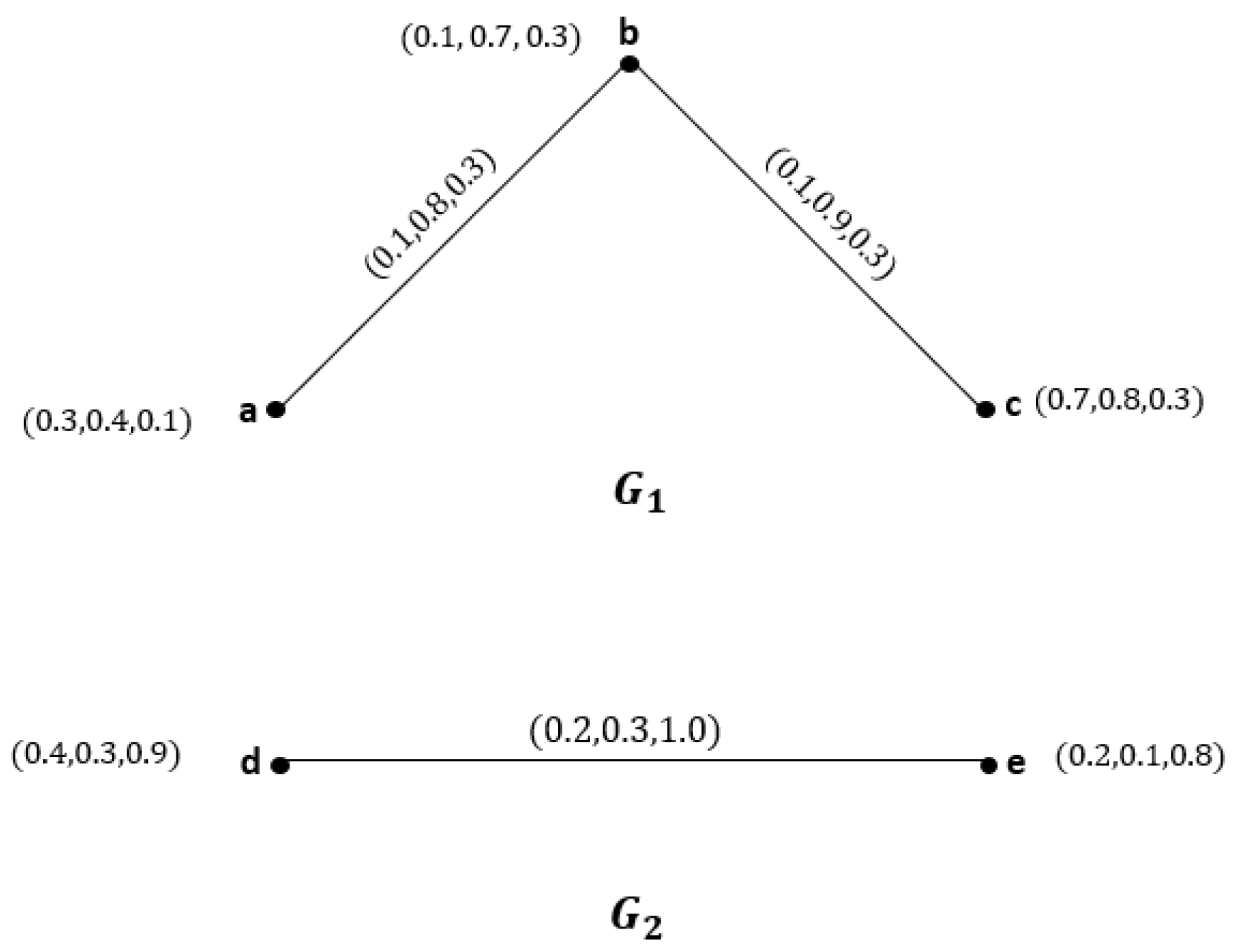
2. 

Moreover, in the context of G, the functions $T^R\stackrel{`}{{\varrho }_{\Re }},I^N\stackrel{`}{{\varrho }_{\Re }}$ and $F^S\stackrel{`}{{\varrho }_{\Re }}$ are mappings from $V\times V$ to the closed interval [0, 1], representing the degrees of true, intermediate, and false membership, in that order for each edge $({\stackrel{`}{\omega }}_i,{\stackrel{`}{\omega }}_j)\in E$.

$$\begin{gathered} T^R\stackrel{`}{{\varrho }_{\Re }}\left({\stackrel{`}{\omega }}_i{\stackrel{`}{\omega }}_j\right)\le T^R{\sigma }_Q\left({\stackrel{`}{\omega }}_i\right)\wedge T^R{\sigma }_Q\left({\stackrel{`}{\omega }}_j\right), \\ {I}^N\stackrel{`}{{\varrho }_{\Re }}\left({\stackrel{`}{\omega }}_i{\stackrel{`}{\omega }}_j\right)\le I^N{\sigma }_Q\left({\stackrel{`}{\omega }}_i\right)\wedge I^N{\sigma }_Q\left({\stackrel{`}{\omega }}_j\right), \\ {F}^S\stackrel{`}{{\varrho }_{\Re }}\left({\stackrel{`}{\omega }}_i{\stackrel{`}{\omega }}_j\right)\ge F^S{\sigma }_Q\left({\stackrel{`}{\omega }}_i\right)\vee F^S{\sigma }_Q\left({\stackrel{`}{\omega }}_j\right). \end{gathered}$$

$0\le T{\sigma }_{\Re }\left({\stackrel{`}{\omega }}_i{\stackrel{`}{\omega }}_j\right)+I{\sigma }_{\Re }\left({\stackrel{`}{\omega }}_i{\stackrel{`}{\omega }}_j\right)+F{\sigma }_{\Re }\left({\stackrel{`}{\omega }}_i{\stackrel{`}{\omega }}_j\right)\le 3$.

Definition 2

([20]). A neutrsophic graph with a subordinate set V is defined to be a pair $G=〈Q,\Re 〉$, where A is a neutrosophic set on $E\subseteq V\times V$ such that

$$\begin{array}{cc}\hfill T^R{\stackrel{`}{\varrho }}_{\Re }(\stackrel{`}{\omega },\stackrel{`}{\upsilon })& \le \wedge \{T^R{\stackrel{`}{\varrho }}_Q\left(\stackrel{`}{\omega }\right),T^R{\stackrel{`}{\varrho }}_Q\left(\stackrel{`}{\upsilon }\right)\}\hfill \\ \hfill I^N{\stackrel{`}{\varrho }}_{\Re }(\stackrel{`}{\omega },\stackrel{`}{\upsilon })& \le \wedge \{I^N{\stackrel{`}{\varrho }}_Q\left(\stackrel{`}{\omega }\right),I^N{\stackrel{`}{\varrho }}_Q\left(\stackrel{`}{\upsilon }\right)\}\hfill \\ \hfill F^S{\stackrel{`}{\varrho }}_{\Re }(\stackrel{`}{\omega },\stackrel{`}{\upsilon })& \ge \vee \{F^S{\stackrel{`}{\varrho }}_Q\left(\stackrel{`}{\omega }\right),F^S{\stackrel{`}{\varrho }}_Q\left(\stackrel{`}{\upsilon }\right)\}\hfill \end{array}$$

for all $\stackrel{`}{\omega },\stackrel{`}{\upsilon }\in V.$

Definition 3.

Let $G=〈Q,\Re 〉$ be a $\aleph G$. The order of a $\aleph G$ is defined by  $O\left(G\right)=({\sum }_{\stackrel{`}{\omega }\in V}{T}^R{\stackrel{`}{\varrho }}_Q\left(\stackrel{`}{\omega }\right),{\sum }_{\stackrel{`}{\omega }\in V}{I}^N{\stackrel{`}{\varrho }}_Q\left(\stackrel{`}{\omega }\right),{\sum }_{\stackrel{`}{\omega }\in V}{F}^S{\stackrel{`}{\varrho }}_Q\left(\stackrel{`}{\omega }\right))$ and the degree of a vertex $\stackrel{`}{\omega }$ in G is defined by $D\left(G\right)=({\sum }_{\stackrel{`}{\omega }\in \Re }{T}^R{\stackrel{`}{\varrho }}_{\Re }\left(\stackrel{`}{\omega }\stackrel{`}{\upsilon }\right),{\sum }_{\stackrel{`}{\omega }\in \Re }{I}^N{\stackrel{`}{\varrho }}_{\Re }\left(\stackrel{`}{\omega }\stackrel{`}{\upsilon }\right),{\sum }_{\stackrel{`}{\omega }\in \Re }{F}^S{\stackrel{`}{\varrho }}_{\Re }\left(\stackrel{`}{\omega }\stackrel{`}{\upsilon }\right))$.

Example 1.

Let $A=\{a,b,c,d\}$ and $B=\{ab,ac,cd\}$ on $G=〈Q,\Re 〉.$ Let A be a $\aleph G$-subset of Q, and let B be a $\aleph G$-subset of $E\subseteq V\times V,$ as given:

$A=(\frac{(0.2,0.4,0.7)}{a},\frac{(0.4,0.8,0.3)}{b},\frac{(0.9,0.7,0.2)}{c},\frac{(0.3,0.1,0.3)}{d})$

$B=(\frac{(0.1,0.7,0.6)}{ab},\frac{(0.1,0.3,0.5)}{ac},\frac{(0.3,0.7,0.2)}{bc},\frac{(0.1,0.3,0.6)}{ad}).$

1. 

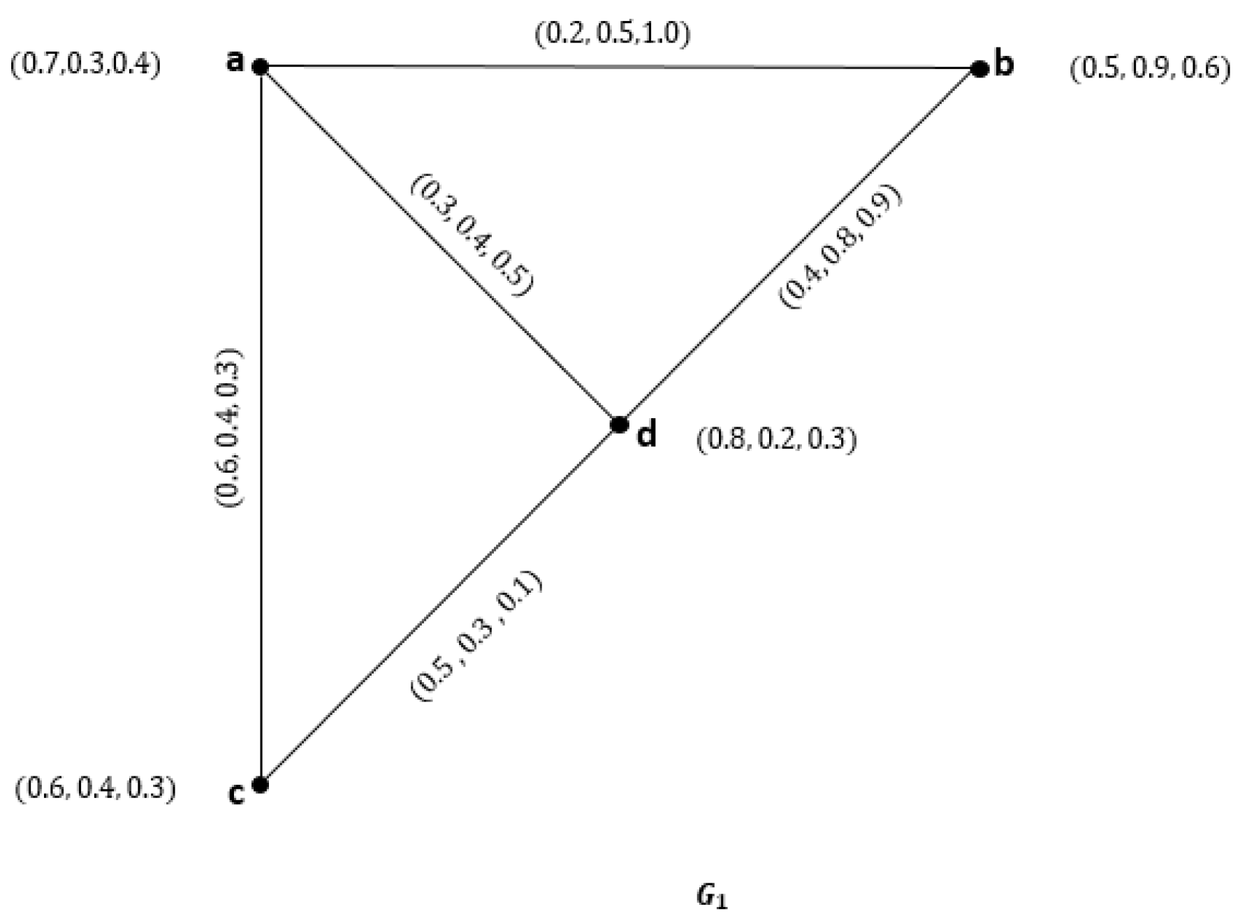
Figure 1 is a $\aleph G$, as may be observed from basic computations.

2. 

$O\left(G\right)=(1.8,2.0,1.5)$

3. 

Each vertex in G has a degree of

• D(a) = (0.2, 1.0, 1.2)
• D(b) = (0.4, 1.4, 0.8)
• D(c) = (0.4, 1.0, 0.7)
• D(d) = (0.1, 0.3, 0.6)

Definition 4.

A pair $G_1\times G_2=〈{\Re }_1\times {\Re }_2,Q_1\times Q_2〉$ is the Cartesian product $G_1\times G_2$ of two $\aleph G$s in order

$$\begin{array}{cc}\hfill 1.T^R{\stackrel{`}{\varrho }}_{{\Re }_1\times {\Re }_2}({\stackrel{`}{\omega }}_1,{\stackrel{`}{\omega }}_2)& =\wedge \{T^R{\stackrel{`}{\varrho }}_{{\Re }_1}\left({\stackrel{`}{\omega }}_1\right),T^R{\stackrel{`}{\varrho }}_{{\Re }_2}\left({\stackrel{`}{\omega }}_2\right)\}\hfill \\ \hfill I^N{\stackrel{`}{\varrho }}_{{\Re }_1\times {\Re }_2}({\stackrel{`}{\omega }}_1,{\stackrel{`}{\omega }}_2)& =\wedge \{I^N{\stackrel{`}{\varrho }}_{{\Re }_1}\left({\stackrel{`}{\omega }}_1\right),I^N{\stackrel{`}{\varrho }}_{{\Re }_2}\left({\stackrel{`}{\omega }}_2\right)\}\hfill \\ \hfill F^S{\stackrel{`}{\varrho }}_{{\Re }_1\times {\Re }_2}({\stackrel{`}{\omega }}_1,{\stackrel{`}{\omega }}_2)& =\vee \{F^S{\stackrel{`}{\varrho }}_{{\Re }_1}\left({\stackrel{`}{\omega }}_1\right),F^S{\stackrel{`}{\varrho }}_{{\Re }_2}\left({\stackrel{`}{\omega }}_2\right)\}\hfill \end{array}$$

for all ${\stackrel{`}{\omega }}_1,{\stackrel{`}{\omega }}_2\in V,$

$$\begin{array}{cc}\hfill 2.T^R{\stackrel{`}{\varrho }}_{Q_1\times Q_2}({\stackrel{`}{\omega }}_1,{\stackrel{`}{\omega }}_2)& =\wedge \{T^R{\stackrel{`}{\varrho }}_{Q_1}\left({\stackrel{`}{\omega }}_1\right),T^R{\stackrel{`}{\varrho }}_{Q_2}\left({\stackrel{`}{\omega }}_2\right)\}\hfill \\ \hfill I^N{\stackrel{`}{\varrho }}_{Q_1\times Q_2}({\stackrel{`}{\omega }}_1,{\stackrel{`}{\omega }}_2)& =\wedge \{I^N{\stackrel{`}{\varrho }}_{Q_1}\left({\stackrel{`}{\omega }}_1\right),I^N{\stackrel{`}{\varrho }}_{Q_2}\left({\stackrel{`}{\omega }}_2\right)\}\hfill \\ \hfill F^S{\stackrel{`}{\varrho }}_{Q_1\times Q_2}({\stackrel{`}{\omega }}_1,{\stackrel{`}{\omega }}_2)& =\vee \{F^S{\stackrel{`}{\varrho }}_{Q_1}\left({\stackrel{`}{\omega }}_1\right),F^S{\stackrel{`}{\varrho }}_{Q_2}\left({\stackrel{`}{\omega }}_2\right)\}\hfill \end{array}$$

for all ${\stackrel{`}{\omega }}_1\in V_1$ and ${\stackrel{`}{\omega }}_2{\stackrel{`}{\upsilon }}_2\in E_2$,

$$\begin{array}{cc}\hfill 3.T^R{\stackrel{`}{\varrho }}_{Q_1\times Q_2}(({\stackrel{`}{\omega }}_1,\stackrel{`}{t}),({\stackrel{`}{\upsilon }}_1,\stackrel{`}{t}))& =\wedge \{T^R{\stackrel{`}{\varrho }}_{Q_1}\left({\stackrel{`}{\omega }}_1{\stackrel{`}{\upsilon }}_1\right),T^R{\stackrel{`}{\varrho }}_{Q_2}\left(\stackrel{`}{t}\right)\}\hfill \\ \hfill I^N{\stackrel{`}{\varrho }}_{Q_1\times Q_2}(({\stackrel{`}{\omega }}_1,\stackrel{`}{t}),({\stackrel{`}{\upsilon }}_1,\stackrel{`}{t}))& =\wedge \{I^N{\stackrel{`}{\varrho }}_{Q_1}\left({\stackrel{`}{\omega }}_1{\stackrel{`}{\upsilon }}_1\right),I^N{\stackrel{`}{\varrho }}_{Q_2}\left(\stackrel{`}{t}\right)\}\hfill \\ \hfill F^S{\stackrel{`}{\varrho }}_{Q_1\times Q_2}(({\stackrel{`}{\omega }}_1,\stackrel{`}{t}),({\stackrel{`}{\upsilon }}_1,\stackrel{`}{t}))& =\vee \{F^S{\stackrel{`}{\varrho }}_{Q_1}\left({\stackrel{`}{\omega }}_1{\stackrel{`}{\upsilon }}_1\right),F^S{\stackrel{`}{\varrho }}_{Q_2}\left(\stackrel{`}{t}\right)\}\hfill \end{array}$$

for all $\stackrel{`}{t}\in V_2$ and ${\stackrel{`}{\omega }}_1{\stackrel{`}{\upsilon }}_1\in E_1$.

Example 2.

Consider the two $\aleph Gs$ $G_1$ and $G_2$, as shown in Figure 2.

Then, their corresponding Cartesian product $〈G_1\times G_2〉$ is shown in Figure 3.

Theorem 1.

A $\aleph G$ can be obtained by taking the Cartesian product of two $\aleph G$s.

Proof. 

Since ${\Re }_1\times {\Re }_2$ has clear criteria, we just check the conditions for $Q_1\times Q_2$.

Let $\stackrel{`}{\omega }\in V_1,$ and ${\stackrel{`}{\omega }}_2{\stackrel{`}{\upsilon }}_2\in E_2$. Then, $T^R{\stackrel{`}{\varrho }}_{Q_1\times Q_2}((\stackrel{`}{\omega },{\stackrel{`}{\omega }}_2),(\stackrel{`}{\omega },{\stackrel{`}{\upsilon }}_2))$

$$\begin{array}{ccc}& =& \wedge \{T^R{\stackrel{`}{\varrho }}_{{\Re }_1}\left(\stackrel{`}{\omega }\right),T^R{\stackrel{`}{\varrho }}_{Q_2}\left({\stackrel{`}{\omega }}_2{\stackrel{`}{\upsilon }}_2\right))\}\hfill \\ & \le & \wedge \{T^R{\stackrel{`}{\varrho }}_{{\Re }_1}\left(\stackrel{`}{\omega }\right),\wedge \left\{T^R{\stackrel{`}{\varrho }}_{Q_2}({\stackrel{`}{\omega }}_2,{\stackrel{`}{\upsilon }}_2)\right\}\}\hfill \\ & =& \wedge \{\wedge \{T^R{\stackrel{`}{\varrho }}_{{\Re }_1}\left(\stackrel{`}{\omega }\right),T^R{\stackrel{`}{\varrho }}_{{\Re }_2}\left({\stackrel{`}{\omega }}_2\right)\},\wedge \{T^R{\stackrel{`}{\varrho }}_{{\Re }_1}\left(\stackrel{`}{\omega }\right),T^R{\stackrel{`}{\varrho }}_{{\Re }_2}\left({\stackrel{`}{\upsilon }}_2\right)\}\}\hfill \\ & =& \wedge \{T^R{\stackrel{`}{\varrho }}_{{\Re }_1\times {\Re }_2}(\stackrel{`}{\omega },{\stackrel{`}{\omega }}_2),T^R{\stackrel{`}{\varrho }}_{{\Re }_1\times {\Re }_2}(\stackrel{`}{\omega },{\stackrel{`}{\upsilon }}_2)\}\hfill \end{array}$$

$I^N{\stackrel{`}{\varrho }}_{Q_1\times Q_2}((\stackrel{`}{\omega },{\stackrel{`}{\omega }}_2),(\stackrel{`}{\omega },{\stackrel{`}{\upsilon }}_2))$

$$\begin{array}{ccc}& =& \wedge \{I^N{\stackrel{`}{\varrho }}_{{\Re }_1}\left(\stackrel{`}{\omega }\right),I^N{\stackrel{`}{\varrho }}_{Q_2}\left({\stackrel{`}{\omega }}_2{\stackrel{`}{\upsilon }}_2\right))\}\hfill \\ & \le & \wedge \{I^N{\stackrel{`}{\varrho }}_{{\Re }_1}\left(\stackrel{`}{\omega }\right),\wedge \left\{I^N{\stackrel{`}{\varrho }}_{Q_2}({\stackrel{`}{\omega }}_2,{\stackrel{`}{\upsilon }}_2)\right\}\}\hfill \\ & =& \wedge \{\wedge \{I^N{\stackrel{`}{\varrho }}_{{\Re }_1}\left(\stackrel{`}{\omega }\right),I^N{\stackrel{`}{\varrho }}_{{\Re }_2}\left({\stackrel{`}{\omega }}_2\right)\},\wedge \{I^N{\stackrel{`}{\varrho }}_{{\Re }_1}\left(\stackrel{`}{\omega }\right),I^N{\stackrel{`}{\varrho }}_{{\Re }_2}\left({\stackrel{`}{\upsilon }}_2\right)\}\},\hfill \\ & =& \wedge \{I^N{\stackrel{`}{\varrho }}_{{\Re }_1\times {\Re }_2}(\stackrel{`}{\omega },{\stackrel{`}{\omega }}_2),I^N{\stackrel{`}{\varrho }}_{{\Re }_1\times {\Re }_2}(\stackrel{`}{\omega },{\stackrel{`}{\upsilon }}_2)\}\hfill \end{array}$$

$F^S{\stackrel{`}{\varrho }}_{Q_1\times Q_2}((\stackrel{`}{\omega },{\stackrel{`}{\omega }}_2),(\stackrel{`}{\omega },{\stackrel{`}{\upsilon }}_2))$

$$\begin{array}{ccc}& =& \vee \{F^S{\stackrel{`}{\varrho }}_{{\Re }_1}\left(\stackrel{`}{\omega }\right),F^S{\stackrel{`}{\varrho }}_{Q_2}\left({\stackrel{`}{\omega }}_2{\stackrel{`}{\upsilon }}_2\right))\}\hfill \\ & \le & \vee \{F^S{\stackrel{`}{\varrho }}_{{\Re }_1}\left(\stackrel{`}{\omega }\right),\vee \left\{F^S{\stackrel{`}{\varrho }}_{Q_2}({\stackrel{`}{\omega }}_2,{\stackrel{`}{\upsilon }}_2)\right\}\}\hfill \\ & =& \vee \{\vee \{F^S{\stackrel{`}{\varrho }}_{{\Re }_1}\left(\stackrel{`}{\omega }\right),F^S{\stackrel{`}{\varrho }}_{{\Re }_2}\left({\stackrel{`}{\omega }}_2\right)\},\vee \{F^S{\stackrel{`}{\varrho }}_{{\Re }_1}\left(\stackrel{`}{\omega }\right),F^S{\stackrel{`}{\varrho }}_{{\Re }_2}\left({\stackrel{`}{\upsilon }}_2\right)\}\},\hfill \\ & =& \vee \{F^S{\gamma }_{{\Re }_1\times {\Re }_2}(\stackrel{`}{\omega },{\stackrel{`}{\omega }}_2),F^S{\gamma }_{{\Re }_1\times {\Re }_2}(\stackrel{`}{\omega },{\stackrel{`}{\upsilon }}_2)\}\hfill \end{array}$$

In the same way, we may establish it for $\stackrel{`}{t}\in V_2$ & ${\stackrel{`}{\omega }}_1{\stackrel{`}{\upsilon }}_1\in E_1.$ □

Definition 5.

Let $G_1\times G_2$ be a $\aleph G$s. The degree of a vertex in $G_1\times G_2$ can be defined as follows: for any $({\stackrel{`}{\omega }}_1,{\stackrel{`}{\omega }}_2)\in V_1\times V_2$, $D_{G_1\times G_2}({\stackrel{`}{\omega }}_1,{\stackrel{`}{\omega }}_2)=({\sum }_{({\stackrel{`}{\omega }}_1,{\stackrel{`}{\omega }}_2)({\stackrel{`}{\upsilon }}_1,{\stackrel{`}{\upsilon }}_2)\in E}{T}^R{\stackrel{`}{\varrho }}_{Q_1\times Q_2}(({\stackrel{`}{\omega }}_1,{\stackrel{`}{\omega }}_2),({\stackrel{`}{\upsilon }}_1,{\stackrel{`}{\upsilon }}_2))$, ${\sum }_{({\stackrel{`}{\omega }}_1,{\stackrel{`}{\omega }}_2)({\stackrel{`}{\upsilon }}_1,{\stackrel{`}{\upsilon }}_2)\in E}{I}^N{\stackrel{`}{\varrho }}_{Q_1\times Q_2}(({\stackrel{`}{\omega }}_1,{\stackrel{`}{\omega }}_2),({\stackrel{`}{\upsilon }}_1,{\stackrel{`}{\upsilon }}_2)),{\sum }_{({\stackrel{`}{\omega }}_1,{\stackrel{`}{\omega }}_2)({\stackrel{`}{\upsilon }}_1,{\stackrel{`}{\upsilon }}_2)\in E}{F}^S{\stackrel{`}{\varrho }}_{Q_1\times Q_2}(({\stackrel{`}{\omega }}_1,{\stackrel{`}{\omega }}_2),({\stackrel{`}{\upsilon }}_1,{\stackrel{`}{\upsilon }}_2))).$

Definition 6.

A pair $G_1\circ G_2=〈{\Re }_1\circ {\Re }_2,Q_1\circ Q_2〉$ is the composition $G_1\circ G_2$ containing two $\aleph G$s, in which case

$$\begin{array}{c}\hfill 1.T^R{\stackrel{`}{\varrho }}_{{\Re }_1\circ {\Re }_2}\left(({\stackrel{`}{\omega }}_1,{\stackrel{`}{\omega }}_2)\right)=\wedge \{T^R{\stackrel{`}{\varrho }}_{{\Re }_1}\left({\stackrel{`}{\omega }}_1\right),T^R{\stackrel{`}{\varrho }}_{{\Re }_1}\left({\stackrel{`}{\omega }}_2\right)\}\\ \hfill I^N{\stackrel{`}{\varrho }}_{{\Re }_1\circ {\Re }_2}\left(({\stackrel{`}{\omega }}_1,{\stackrel{`}{\omega }}_2)\right)=\wedge \{I^N{\stackrel{`}{\varrho }}_{{\Re }_1}\left({\stackrel{`}{\omega }}_1\right),I^N{\stackrel{`}{\varrho }}_{{\Re }_1}\left({\stackrel{`}{\omega }}_2\right)\}\\ \hfill F^S{\stackrel{`}{\varrho }}_{{\Re }_1\circ {\Re }_2}\left(({\stackrel{`}{\omega }}_1,{\stackrel{`}{\omega }}_2)\right)=\vee \{F^S{\stackrel{`}{\varrho }}_{{\Re }_1}\left({\stackrel{`}{\omega }}_1\right),F^S{\stackrel{`}{\varrho }}_{{\Re }_1}\left({\stackrel{`}{\omega }}_2\right)\}\end{array}$$

for all ${\stackrel{`}{\omega }}_1,{\stackrel{`}{\omega }}_2\in V$,

$$\begin{array}{c}\hfill 2.T^R{\stackrel{`}{\varrho }}_{Q_1\circ Q_2}\left(({\stackrel{`}{\omega }}_1,{\stackrel{`}{\omega }}_2)\right)=\wedge \{T^R{\stackrel{`}{\varrho }}_{Q_1}\left({\stackrel{`}{\omega }}_1\right),T^R{\stackrel{`}{\varrho }}_{Q_1}\left({\stackrel{`}{\omega }}_2\right)\}\\ \hfill I^N{\stackrel{`}{\varrho }}_{Q_1\circ Q_2}\left(({\stackrel{`}{\omega }}_1,{\stackrel{`}{\omega }}_2)\right)=\wedge \{I^N{\stackrel{`}{\varrho }}_{Q_1}\left({\stackrel{`}{\omega }}_1\right),I^N{\stackrel{`}{\varrho }}_{Q_1}\left({\stackrel{`}{\omega }}_2\right)\}\\ \hfill F^S{\stackrel{`}{\varrho }}_{Q_1\circ Q_2}\left(({\stackrel{`}{\omega }}_1,{\stackrel{`}{\omega }}_2)\right)=\vee \{F^S{\stackrel{`}{\varrho }}_{Q_1}\left({\stackrel{`}{\omega }}_1\right),F^S{\stackrel{`}{\varrho }}_{Q_1}\left({\stackrel{`}{\omega }}_2\right)\}\end{array}$$

for all ${\stackrel{`}{\omega }}_1\in V_1,$ and ${\stackrel{`}{\omega }}_2{\stackrel{`}{\upsilon }}_2\in E_2$,

$$\begin{array}{c}\hfill 3.T^R{\stackrel{`}{\varrho }}_{Q_1\circ Q_2}\left(({\stackrel{`}{\omega }}_1,\stackrel{`}{t})({\stackrel{`}{\upsilon }}_1,\stackrel{`}{t})\right)=\wedge \{T^R{\stackrel{`}{\varrho }}_{Q_1}\left({\stackrel{`}{\omega }}_1{\stackrel{`}{\upsilon }}_1\right),T^R{\stackrel{`}{\varrho }}_{{\Re }_2}\left(\stackrel{`}{t}\right)\}\\ \hfill I^N{\stackrel{`}{\varrho }}_{Q_1\circ Q_2}\left(({\stackrel{`}{\omega }}_1,\stackrel{`}{t})({\stackrel{`}{\upsilon }}_1,\stackrel{`}{t})\right)=\wedge \{I^N{\stackrel{`}{\varrho }}_{Q_1}\left({\stackrel{`}{\omega }}_1{\stackrel{`}{\upsilon }}_1\right),I^N{\stackrel{`}{\varrho }}_{{\Re }_2}\left(\stackrel{`}{t}\right)\}\\ \hfill F^S{\stackrel{`}{\varrho }}_{Q_1\circ Q_2}\left(({\stackrel{`}{\omega }}_1,\stackrel{`}{t})({\stackrel{`}{\upsilon }}_1,\stackrel{`}{t})\right)=\vee \{F^S{\stackrel{`}{\varrho }}_{Q_1}\left({\stackrel{`}{\omega }}_1{\stackrel{`}{\upsilon }}_1\right),F^S{\stackrel{`}{\varrho }}_{{\Re }_2}\left(\stackrel{`}{t}\right)\}\end{array}$$

for all $\stackrel{`}{t}\in V_2,$ and ${\stackrel{`}{\omega }}_1{\stackrel{`}{\upsilon }}_1\in E_1$,

$$\begin{array}{c}\hfill 4.T^R{\stackrel{`}{\varrho }}_{Q_1\circ Q_2}\left(({\stackrel{`}{\omega }}_1,{\stackrel{`}{\omega }}_2)({\stackrel{`}{\upsilon }}_1,{\stackrel{`}{\upsilon }}_2)\right)=\wedge \{T^R{\stackrel{`}{\varrho }}_{{\Re }_2}\left({\stackrel{`}{\omega }}_2\right),T^R{\stackrel{`}{\varrho }}_{{\Re }_2}\left({\stackrel{`}{\upsilon }}_2\right),T^R{\stackrel{`}{\varrho }}_{Q_1}\left({\stackrel{`}{\omega }}_1{\stackrel{`}{\upsilon }}_1\right)\}\\ \hfill I^N{\stackrel{`}{\varrho }}_{Q_1\circ Q_2}\left(({\stackrel{`}{\omega }}_1,{\stackrel{`}{\omega }}_2)({\stackrel{`}{\upsilon }}_1,{\stackrel{`}{\upsilon }}_2)\right)=\wedge \{I^N{\stackrel{`}{\varrho }}_{{\Re }_2}\left({\stackrel{`}{\omega }}_2\right),I^N{\stackrel{`}{\varrho }}_{{\Re }_2}\left({\stackrel{`}{\upsilon }}_2\right),I^N{\stackrel{`}{\varrho }}_{Q_1}\left({\stackrel{`}{\omega }}_1{\stackrel{`}{\upsilon }}_1\right)\}\\ \hfill F^S{\stackrel{`}{\varrho }}_{Q_1\circ Q_2}\left(({\stackrel{`}{\omega }}_1,{\stackrel{`}{\omega }}_2)({\stackrel{`}{\upsilon }}_1,{\stackrel{`}{\upsilon }}_2)\right)=\vee \{F^S{\stackrel{`}{\varrho }}_{{\Re }_2}\left({\stackrel{`}{\omega }}_2\right),F^S{\stackrel{`}{\varrho }}_{{\Re }_2}\left({\stackrel{`}{\upsilon }}_2\right),F^S{\stackrel{`}{\varrho }}_{Q_1}\left({\stackrel{`}{\omega }}_1{\stackrel{`}{\upsilon }}_1\right)\}\end{array}$$

for all ${\stackrel{`}{\omega }}_2,{\stackrel{`}{\upsilon }}_2\in V_2,{\stackrel{`}{\omega }}_2\ne {\stackrel{`}{\upsilon }}_2$ and ${\stackrel{`}{\omega }}_1{\stackrel{`}{\upsilon }}_1\in E_1$.

Definition 7.

Let $G_1\circ G_2$ be a $\aleph G$. The degree of a vertex in $G_1\circ G_2$ can be defined as follows: for any $({\stackrel{`}{\omega }}_1,{\stackrel{`}{\omega }}_2)\in V_1\circ V_2$,

$D_{G_1\circ G_2}({\stackrel{`}{\omega }}_1,{\stackrel{`}{\omega }}_2)=$

$({\sum }_{({\stackrel{`}{\omega }}_1,{\stackrel{`}{\omega }}_2)({\stackrel{`}{\upsilon }}_1,{\stackrel{`}{\upsilon }}_2)\in E}{T}^R{\stackrel{`}{\varrho }}_{Q_1\circ Q_2}(({\stackrel{`}{\omega }}_1,{\stackrel{`}{\omega }}_2),({\stackrel{`}{\upsilon }}_1,{\stackrel{`}{\upsilon }}_2)),$

${\sum }_{({\stackrel{`}{\omega }}_1,{\stackrel{`}{\omega }}_2)({\stackrel{`}{\upsilon }}_1,{\stackrel{`}{\upsilon }}_2)\in E}{I}^N{\stackrel{`}{\varrho }}_{Q_1\circ Q_2}(({\stackrel{`}{\omega }}_1,{\stackrel{`}{\omega }}_2),({\stackrel{`}{\upsilon }}_1,{\stackrel{`}{\upsilon }}_2)),$

${\sum }_{({\stackrel{`}{\omega }}_1,{\stackrel{`}{\omega }}_2)({\stackrel{`}{\upsilon }}_1,{\stackrel{`}{\upsilon }}_2)\in E}{F}^S{\stackrel{`}{\varrho }}_{Q_1\circ Q_2}(({\stackrel{`}{\omega }}_1,{\stackrel{`}{\omega }}_2),({\stackrel{`}{\upsilon }}_1,{\stackrel{`}{\upsilon }}_2)))$.

Example 3.

Consider the two $\aleph G$, as shown in Figure 4

Then, their composition $G_1\circ G_2$ is shown in Figure 5.

Definition 8.

Given two $\aleph G$s, the union $G_1\cup G_2=〈{\Re }_1\cup {\Re }_2,Q_1\cup Q_2〉$ is described below:

1. 

$T^R{\stackrel{`}{\varrho }}_{{\Re }_1\cup {\Re }_2}\left(\stackrel{`}{\omega }\right)=T^R{\stackrel{`}{\varrho }}_{{\Re }_1}\left(\stackrel{`}{\omega }\right)$

$I^N{\stackrel{`}{\varrho }}_{{\Re }_1\cup {\Re }_2}\left(\stackrel{`}{\omega }\right)=I^N{\stackrel{`}{\varrho }}_{{\Re }_1}\left(\stackrel{`}{\omega }\right)$

$F^S{\stackrel{`}{\varrho }}_{{\Re }_1\cup {\Re }_2}\left(\stackrel{`}{\omega }\right)=F^S{\stackrel{`}{\varrho }}_{{\Re }_1}\left(\stackrel{`}{\omega }\right)$, for $\stackrel{`}{\omega }\in V_1$ & $\stackrel{`}{\omega }\notin V_2$.

2. 

$T^R{\stackrel{`}{\varrho }}_{{\Re }_1\cup {\Re }_2}\left(\stackrel{`}{\omega }\right)=T^R{\stackrel{`}{\varrho }}_{{\Re }_2}\left(\stackrel{`}{\omega }\right)$

$I^N{\stackrel{`}{\varrho }}_{{\Re }_1\cup {\Re }_2}\left(\stackrel{`}{\omega }\right)=I^N{\stackrel{`}{\varrho }}_{{\Re }_2}\left(\stackrel{`}{\omega }\right)$

$F^S{\stackrel{`}{\varrho }}_{{\Re }_1\cup {\Re }_2}\left(\stackrel{`}{\omega }\right)=F^S{\stackrel{`}{\varrho }}_{{\Re }_2}\left(\stackrel{`}{\omega }\right)$, for $\stackrel{`}{\omega }\in V_2$ & $\stackrel{`}{\omega }\notin V_1$.

3. 

$T^R{\stackrel{`}{\varrho }}_{{\Re }_1\cup {\Re }_2}\left(\stackrel{`}{\omega }\right)=\vee \{T^R{\stackrel{`}{\varrho }}_{{\Re }_2}\left(\stackrel{`}{\omega }\right),T^R{\stackrel{`}{\varrho }}_{{\Re }_2}\left(\stackrel{`}{\omega }\right)\}$

$I^N{\stackrel{`}{\varrho }}_{{\Re }_1\cup {\Re }_2}\left(\stackrel{`}{\omega }\right)=\vee \{I^N{\stackrel{`}{\varrho }}_{{\Re }_2}\left(\stackrel{`}{\omega }\right),I^N{\stackrel{`}{\varrho }}_{{\Re }_2}\left(\stackrel{`}{\omega }\right)\}$

$F^S{\stackrel{`}{\varrho }}_{{\Re }_1\cup {\Re }_2}\left(\stackrel{`}{\omega }\right)=\wedge \{I^N{\stackrel{`}{\varrho }}_{{\Re }_2}\left(\stackrel{`}{\omega }\right),F^S{\stackrel{`}{\varrho }}_{{\Re }_2}\left(\stackrel{`}{\omega }\right)\}$.

4. 

$T^R{\stackrel{`}{\varrho }}_{Q_1\cup Q_2}\left(\stackrel{`}{\omega }\stackrel{`}{\upsilon }\right)=T^R{\stackrel{`}{\varrho }}_{Q_1}\left(\stackrel{`}{\omega }\stackrel{`}{\upsilon }\right)$

$I^N{\stackrel{`}{\varrho }}_{Q_1\cup Q_2}\left(\stackrel{`}{\omega }\stackrel{`}{\upsilon }\right)=I^N{\stackrel{`}{\varrho }}_{Q_1}\left(\stackrel{`}{\omega }\stackrel{`}{\upsilon }\right)$

$F^S{\stackrel{`}{\varrho }}_{Q_1\cup Q_2}\left(\stackrel{`}{\omega }\stackrel{`}{\upsilon }\right)=F^S{\stackrel{`}{\varrho }}_{Q_1}\left(\stackrel{`}{\omega }\stackrel{`}{\upsilon }\right)$, for $\stackrel{`}{\omega }\stackrel{`}{\upsilon }\in E_1$ & $\stackrel{`}{\omega }\stackrel{`}{\upsilon }\notin E_2$.

5. 

$T^R{\stackrel{`}{\varrho }}_{Q_1\cup Q_2}\left(\stackrel{`}{\omega }\stackrel{`}{\upsilon }\right)=T^R{\stackrel{`}{\varrho }}_{Q_2}\left(\stackrel{`}{\omega }\stackrel{`}{\upsilon }\right)$

$I^N{\stackrel{`}{\varrho }}_{Q_1\cup Q_2}\left(\stackrel{`}{\omega }\stackrel{`}{\upsilon }\right)=I^N{\stackrel{`}{\varrho }}_{Q_2}\left(\stackrel{`}{\omega }\stackrel{`}{\upsilon }\right)$

$F^S{\stackrel{`}{\varrho }}_{Q_1\cup Q_2}\left(\stackrel{`}{\omega }\stackrel{`}{\upsilon }\right)=F^S{\stackrel{`}{\varrho }}_{Q_2}\left(\stackrel{`}{\omega }\stackrel{`}{\upsilon }\right)$, for $\stackrel{`}{\omega }\stackrel{`}{\upsilon }\in E_2$ & $\stackrel{`}{\omega }\stackrel{`}{\upsilon }\notin E_1$.

6. 

$T^R{\stackrel{`}{\varrho }}_{Q_1\cup Q_2}\left(\stackrel{`}{\omega }\stackrel{`}{\upsilon }\right)=\vee \{T^R{\stackrel{`}{\varrho }}_{Q_2}\left(\stackrel{`}{\omega }\stackrel{`}{\upsilon }\right),T^R{\stackrel{`}{\varrho }}_{Q_2}\left(\stackrel{`}{\omega }\stackrel{`}{\upsilon }\right)\}$

$I^N{\stackrel{`}{\varrho }}_{Q_1\cup Q_2}\left(\stackrel{`}{\omega }\stackrel{`}{\upsilon }\right)=\vee \{I^N{\stackrel{`}{\varrho }}_{Q_2}\left(\stackrel{`}{\omega }\stackrel{`}{\upsilon }\right),I^N{\stackrel{`}{\varrho }}_{Q_2}\left(\stackrel{`}{\omega }\stackrel{`}{\upsilon }\right)\}$

$F^S{\stackrel{`}{\varrho }}_{Q_1\cup Q_2}\left(\stackrel{`}{\omega }\stackrel{`}{\upsilon }\right)=\wedge \{F^D{\stackrel{`}{\varrho }}_{Q_2}\left(\stackrel{`}{\omega }\stackrel{`}{\upsilon }\right),F^S{\stackrel{`}{\varrho }}_{Q_2}\left(\stackrel{`}{\omega }\stackrel{`}{\upsilon }\right)\}$.

Example 4.

Take a look at the two distinct $\aleph Gs$ presented in Figure 6 as well as Figure 7.

Then, their union $G_1\cup G_2$ is shown in Figure 8.

Definition 9.

Given two $\aleph G$s, $V_1\bigcap V_2=⌀$. The join $G_1+G_2=〈{\Re }_1+{\Re }_2,Q_1+Q_2〉$ is stated below:

1. 

$T^R{\stackrel{`}{\varrho }}_{{\Re }_1+{\Re }_2}\left(\stackrel{`}{\omega }\right)=T^R{\stackrel{`}{\varrho }}_{{\Re }_1\cup {\Re }_2}\left(\stackrel{`}{\omega }\right)$

$I^N{\stackrel{`}{\varrho }}_{{\Re }_1+{\Re }_2}\left(\stackrel{`}{\omega }\right)=I^N{\stackrel{`}{\varrho }}_{{\Re }_1\cup {\Re }_2}\left(\stackrel{`}{\omega }\right)$

$F^S{\stackrel{`}{\varrho }}_{{\Re }_1+{\Re }_2}\left(\stackrel{`}{\omega }\right)=F^S{\stackrel{`}{\varrho }}_{{\Re }_1\cup {\Re }_2}\left(\stackrel{`}{\omega }\right)$, if $\stackrel{`}{\omega }\in V_1\cup V_2$.

2. 

$T^R{\stackrel{`}{\varrho }}_{Q_1+Q_2}\left(\stackrel{`}{\omega }\stackrel{`}{\upsilon }\right)=T^R{\stackrel{`}{\varrho }}_{{\Re }_1\cup {\Re }_2}\left(\stackrel{`}{\omega }\stackrel{`}{\upsilon }\right)$

$I^N{\stackrel{`}{\varrho }}_{Q_1+Q_2}\left(\stackrel{`}{\omega }\stackrel{`}{\upsilon }\right)=I^N{\stackrel{`}{\varrho }}_{{\Re }_1\cup {\Re }_2}\left(\stackrel{`}{\omega }\stackrel{`}{\upsilon }\right)$

$F^S{\stackrel{`}{\varrho }}_{Q_1+Q_2}\left(\stackrel{`}{\omega }\stackrel{`}{\upsilon }\right)=F^S{\stackrel{`}{\varrho }}_{{\Re }_1\cup {\Re }_2}\left(\stackrel{`}{\omega }\stackrel{`}{\upsilon }\right)$, for $\stackrel{`}{\omega }\stackrel{`}{\upsilon }\in E_1\cap E_2$.

3. 

$T^R{\stackrel{`}{\varrho }}_{Q_1+Q_2}\left(\stackrel{`}{\omega }\stackrel{`}{\upsilon }\right)=\wedge \{T^R{\stackrel{`}{\varrho }}_{{\Re }_1}\left(\stackrel{`}{\omega }\right),T^R{\stackrel{`}{\varrho }}_{{\Re }_1}\left(\stackrel{`}{\upsilon }\right)\}$

$I^N{\stackrel{`}{\varrho }}_{Q_1+Q_2}\left(\stackrel{`}{\omega }\stackrel{`}{\upsilon }\right)=\wedge \{I^N{\stackrel{`}{\varrho }}_{{\Re }_1}\left(\stackrel{`}{\omega }\right),I^N{\stackrel{`}{\varrho }}_{{\Re }_1}\left(\stackrel{`}{\upsilon }\right)\}$

$F^S{\stackrel{`}{\varrho }}_{Q_1+Q_2}\left(\stackrel{`}{\omega }\stackrel{`}{\upsilon }\right)=\vee \{F^S{\stackrel{`}{\varrho }}_{{\Re }_1}\left(\stackrel{`}{\omega }\right),F^S{\stackrel{`}{\varrho }}_{{\Re }_1}\left(\stackrel{`}{\upsilon }\right)\}$, if $\stackrel{`}{\omega }\stackrel{`}{\upsilon }\in E$. Where E is the collection of all edges connecting $V_1$ & $V_2$ vertices.

Theorem 2.

Let $G_1=({\Re }_1,Q_1)$ and $G_2=({\Re }_2,Q_2)$ be neutrosophic graphs of the graphs $G_1^{*}$ and $G_2^{*}$ and let $V_1\cap V_2=⌀$. Then, union $G_1\cup G_2=({\Re }_1\cup {\Re }_2,Q_1\cup Q_2)$ is a $\aleph G$ of $G_{*}$ iff $G_1$ and $G_2$ are $\aleph Gs$ of the graphs $G_1^{*}$ and $G_2^{*}$, respectively.

Proof. 

Suppose that $G_1\cup G_2$ is a $\aleph G$. Let $\stackrel{`}{\omega }\stackrel{`}{\upsilon }\notin E_1$ and $\stackrel{`}{\omega },\stackrel{`}{\upsilon }\in V_1-V_2$. Thus,

$$\begin{array}{ccc}\hfill T^R{\stackrel{`}{\varrho }}_{Q_1}\left(\stackrel{`}{\omega }\stackrel{`}{\upsilon }\right)& =& T^R{\stackrel{`}{\varrho }}_{Q_1\cup Q_2}\left(\stackrel{`}{\omega }\stackrel{`}{\upsilon }\right)\hfill \\ & =& \wedge \{T^R{\stackrel{`}{\varrho }}_{{\Re }_1\cap {\Re }_2}\left(\stackrel{`}{\omega }\right),T^R{\stackrel{`}{\varrho }}_{{\Re }_1\cap {\Re }_2}\left(\stackrel{`}{\upsilon }\right)\}\hfill \\ & =& \wedge \{T^R{\stackrel{`}{\varrho }}_{{\Re }_1}\left(\stackrel{`}{\omega }\right),T^R{\stackrel{`}{\varrho }}_{{\Re }_1}\left(\stackrel{`}{\upsilon }\right)\}\hfill \end{array}$$

$$\begin{array}{ccc}\hfill I^N{\stackrel{`}{\varrho }}_{Q_1}\left(\stackrel{`}{\omega }\stackrel{`}{\upsilon }\right)& =& I^N{\stackrel{`}{\varrho }}_{Q_1\cup Q_2}\left(\stackrel{`}{\omega }\stackrel{`}{\upsilon }\right)\hfill \\ & =& \wedge \{I^N{\stackrel{`}{\varrho }}_{{\Re }_1\cap {\Re }_2}\left(\stackrel{`}{\omega }\right),I^N{\stackrel{`}{\varrho }}_{{\Re }_1\cap {\Re }_2}\left(\stackrel{`}{\upsilon }\right)\}\hfill \\ & =& \wedge \{I^N{\stackrel{`}{\varrho }}_{{\Re }_1}\left(\stackrel{`}{\omega }\right),I^N{\stackrel{`}{\varrho }}_{{\Re }_1}\left(\stackrel{`}{\upsilon }\right)\}\hfill \\ \hfill F^S{\stackrel{`}{\varrho }}_{Q_1}\left(\stackrel{`}{\omega }\stackrel{`}{\upsilon }\right)& =& F^S{\stackrel{`}{\varrho }}_{Q_1\cup Q_2}\left(\stackrel{`}{\omega }\stackrel{`}{\upsilon }\right)\hfill \\ & =& \vee \{F^S{\stackrel{`}{\varrho }}_{{\Re }_1\cap {\Re }_2}\left(\stackrel{`}{\omega }\right),F^S{\stackrel{`}{\varrho }}_{{\Re }_1\cap {\Re }_2}\left(\stackrel{`}{\upsilon }\right)\}\hfill \\ & =& \vee \{F^S{\gamma }_{{\Re }_1}\left(\stackrel{`}{\omega }\right),F^S{\gamma }_{{\Re }_1}\left(\stackrel{`}{\upsilon }\right)\}\hfill \end{array}$$

□

This shows that $G_1=({\Re }_1,Q_1)$ is a $\aleph G$, Similarly, we can show that $G_2=({\Re }_2,Q_2)$ is a $\aleph G$. The converse part is obvious.

Theorem 3.

Let $G_1=〈{\Re }_1,Q_1〉$ and $G_2=〈{\Re }_2,Q_2〉$ be $\aleph G$s of the graphs $G_1^{*}$ and $G_2^{*}$, and let $V_1\cap V_2=⌀$. Then, join $G_1+G_2=({\Re }_1+{\Re }_2,Q_1+Q_2)$ is a $\aleph G$ of $G_{*}$ if $G_1$ and $G_2$ are $\aleph Gs$ of the graphs $G_1^{*}$ and $G_2^{*}$.

Proof. 

Proof is similar to the proof of Theorem 2. ☐

3. Isomorphism of $\aleph \mathbf{G}$s

Definition 10.

Let $G_1=〈{\Re }_1,Q_1〉$ and $G_2=〈{\Re }_2,Q_2〉$ be two $\aleph G$s. A homomorphism $g:G_1\to G_2$ is a mapping $g:V_1\to V_2$ such that:

1. 

$\left\{\begin{array}{c}{T}^R{\stackrel{`}{\varrho }}_{{\Re }_1}\left({\stackrel{`}{\omega }}_1\right)\le T^R{\stackrel{`}{\varrho }}_{{\Re }_2}\left(\varpi \left({\stackrel{`}{\omega }}_1\right)\right)\hfill \\ I^N{\stackrel{`}{\varrho }}_{{\Re }_1}\left({\stackrel{`}{\omega }}_1\right)\le I^N{\stackrel{`}{\varrho }}_{{\Re }_2}\left(\varpi \left({\stackrel{`}{\omega }}_1\right)\right)forall{\stackrel{`}{\omega }}_1{\stackrel{`}{\upsilon }}_1\in V_1\hfill \\ F^S{\stackrel{`}{\varrho }}_{{\Re }_1}\left({\stackrel{`}{\omega }}_1\right)\ge F^S{\stackrel{`}{\varrho }}_{{\Re }_2}\left(\varpi \left({\stackrel{`}{\omega }}_1\right)\right)\hfill \end{array}\right.$

2. 

$\left\{\begin{array}{c}{T}^R{\stackrel{`}{\varrho }}_{Q_1}\left({\stackrel{`}{\omega }}_1{\stackrel{`}{\upsilon }}_1\right)\le T^R{\stackrel{`}{\varrho }}_{Q_2}\left(\varpi \left({\stackrel{`}{\omega }}_1\right)\varpi \left({\stackrel{`}{\upsilon }}_1\right)\right)\hfill \\ I^N{\stackrel{`}{\varrho }}_{Q_1}\left({\stackrel{`}{\omega }}_1{\stackrel{`}{\upsilon }}_1\right)\le I^N{\stackrel{`}{\varrho }}_{Q_2}\left(\varpi \left({\stackrel{`}{\omega }}_1\right)\varpi \left({\stackrel{`}{\upsilon }}_1\right)\right)forall{\stackrel{`}{\omega }}_1{\stackrel{`}{\upsilon }}_1\in E_1\hfill \\ F^S{\stackrel{`}{\varrho }}_{Q_1}\left({\stackrel{`}{\omega }}_1{\stackrel{`}{\upsilon }}_1\right)\ge F^S{\stackrel{`}{\varrho }}_{Q_2}\left(\varpi \left({\stackrel{`}{\omega }}_1\right)\varpi \left({\stackrel{`}{\upsilon }}_1\right)\right)\hfill \end{array}\right.$

A bijective homomorphism with the property

3. 

$\left\{\begin{array}{c}{T}^R{\stackrel{`}{\varrho }}_{{\Re }_1}\left({\stackrel{`}{\omega }}_1\right)=T^R{\stackrel{`}{\varrho }}_{{\Re }_2}\left(\varpi \left({\stackrel{`}{\omega }}_1\right)\right)\hfill \\ I^N{\stackrel{`}{\varrho }}_{{\Re }_1}\left({\stackrel{`}{\omega }}_1\right)=I^N{\stackrel{`}{\varrho }}_{{\Re }_2}\left(\varpi \left({\stackrel{`}{\omega }}_1\right)\right)forall{\stackrel{`}{\omega }}_1\in V_1\hfill \\ F^S{\stackrel{`}{\varrho }}_{{\Re }_1}\left({\stackrel{`}{\omega }}_1\right)=F^S{\stackrel{`}{\varrho }}_{{\Re }_2}\left(\varpi \left({\stackrel{`}{\omega }}_1\right)\right)\hfill \end{array}\right.$ is called a week isomorphism.

A bijective homomorphism with the property

4. 

$\left\{\begin{array}{c}{T}^R{\stackrel{`}{\varrho }}_{Q_1}\left({\stackrel{`}{\omega }}_1{\stackrel{`}{\upsilon }}_1\right)=T^R{\stackrel{`}{\varrho }}_{Q_2}\left(\varpi \left({\stackrel{`}{\omega }}_1\right)\varpi \left({\stackrel{`}{\upsilon }}_1\right)\right)\hfill \\ I^N{\stackrel{`}{\varrho }}_{Q_1}\left({\stackrel{`}{\omega }}_1{\stackrel{`}{\upsilon }}_1\right)=I^N{\stackrel{`}{\varrho }}_{Q_2}\left(\varpi \left({\stackrel{`}{\omega }}_1\right)\varpi \left({\stackrel{`}{\upsilon }}_1\right)\right)forall{\stackrel{`}{\omega }}_1{\stackrel{`}{\upsilon }}_1\in E_1\hfill \\ F^S{\stackrel{`}{\varrho }}_{Q_1}\left({\stackrel{`}{\omega }}_1{\stackrel{`}{\upsilon }}_1\right)=F^S{\stackrel{`}{\varrho }}_{Q_2}\left(\varpi \left({\stackrel{`}{\omega }}_1\right)\varpi \left({\stackrel{`}{\upsilon }}_1\right)\right)\hfill \end{array}\right.$ is called a strong co-isomorphism. A bijective mapping $\varpi :G_1\to G_2$ satisfying 3 and 4 is called an isomorphism.

Theorem 4.

An isomorphism between $\aleph Gs$ is an equivalence relation.

Proof. 

Reflexivity and symmetry are obvious. To prove the transitivity, we let $\tau :V_1\to V_2$ and $\varpi :V_2\to V_3$ be the isomorphisms of $G_1$ onto $G_2$ and $G_2$ onto $G_3$, respectively. Then, $\varpi \circ \tau :V_1\to V_3$ is the bijective map from $V_1$ to $V_3$, where $(\varpi \circ \tau )\left({\stackrel{`}{\omega }}_1\right)=\varpi \left(\tau \left({\stackrel{`}{\omega }}_1\right)\right)$ for all ${\stackrel{`}{\omega }}_1\in V_1$. Since a map $\tau :V_1\to V_2$ defined by $\tau \left({\stackrel{`}{\omega }}_1\right)={\stackrel{`}{\omega }}_2$ for ${\stackrel{`}{\omega }}_1\in V_1$ is an isomorphism. Now

$$\begin{array}{cc}\hfill T^R{\stackrel{`}{\varrho }}_{{\Re }_1}\left({\stackrel{`}{\omega }}_1\right)& =T^R{\stackrel{`}{\varrho }}_{{\Re }_2}\left(\tau \left({\stackrel{`}{\omega }}_1\right)\right)\hfill \\ \hfill & =T^R{\stackrel{`}{\varrho }}_{{\Re }_2}\left({\stackrel{`}{\omega }}_2\right),forall{\stackrel{`}{\omega }}_1\in V_1\hfill \\ \hfill I^N{\stackrel{`}{\varrho }}_{{\Re }_1}\left({\stackrel{`}{\omega }}_1\right)& =I^N{\stackrel{`}{\varrho }}_{{\Re }_2}\left(\tau \left({\stackrel{`}{\omega }}_1\right)\right)\hfill \\ \hfill & =I^N{\stackrel{`}{\varrho }}_{{\Re }_2}\left({\stackrel{`}{\omega }}_2\right),forall{\stackrel{`}{\omega }}_1\in V_1\hfill \\ \hfill F^S{\stackrel{`}{\varrho }}_{{\Re }_1}\left({\stackrel{`}{\omega }}_1\right)& =F^S{\stackrel{`}{\varrho }}_{{\Re }_2}\left(\varpi \left({\stackrel{`}{\omega }}_1\right)\right)\hfill \\ \hfill & =F^S{\stackrel{`}{\varrho }}_{{\Re }_2}\left({\stackrel{`}{\omega }}_2\right)e^{i{F}^S{\gamma }_{{\Re }_2}\left({\stackrel{`}{\omega }}_2\right)},forall{\stackrel{`}{\omega }}_1\in V_1\hfill \\ \hfill T^R{\stackrel{`}{\varrho }}_{Q_1}\left({\stackrel{`}{\omega }}_1{\stackrel{`}{\upsilon }}_1\right)& =T^R{\stackrel{`}{\varrho }}_{Q_2}\left(\tau \left({\stackrel{`}{\omega }}_1\right)\tau \left({\stackrel{`}{\upsilon }}_1\right)\right)\hfill \\ \hfill & =T^R{\stackrel{`}{\varrho }}_{Q_2}\left({\stackrel{`}{\omega }}_2{\stackrel{`}{\upsilon }}_2\right),forall{\stackrel{`}{\omega }}_1{\stackrel{`}{\upsilon }}_1\in E_1\hfill \\ \hfill I^N{\stackrel{`}{\varrho }}_{Q_1}\left({\stackrel{`}{\omega }}_1{\stackrel{`}{\upsilon }}_1\right)& =I^N{\stackrel{`}{\varrho }}_{Q_2}\left(\tau \left({\stackrel{`}{\omega }}_1\right)\tau \left({\stackrel{`}{\upsilon }}_1\right)\right)\hfill \\ \hfill & =I^N{\stackrel{`}{\varrho }}_{Q_2}\left({\stackrel{`}{\omega }}_2{\stackrel{`}{\upsilon }}_2\right),forall{\stackrel{`}{\omega }}_1{\stackrel{`}{\upsilon }}_1\in E_1\hfill \\ \hfill F^S{\stackrel{`}{\varrho }}_{Q_1}\left({\stackrel{`}{\omega }}_1{\stackrel{`}{\upsilon }}_1\right)& =F^S{\stackrel{`}{\varrho }}_{Q_2}\left(\tau \left({\stackrel{`}{\omega }}_1\right)\tau \left({\stackrel{`}{\upsilon }}_1\right)\right)\hfill \\ \hfill & =F^S{\stackrel{`}{\varrho }}_{Q_2}\left({\stackrel{`}{\omega }}_2{\stackrel{`}{\upsilon }}_2\right)e^{i{F}^S{\beta }_{Q_2}\left({\stackrel{`}{\omega }}_2{\stackrel{`}{\upsilon }}_2\right)},forall{\stackrel{`}{\omega }}_1{\stackrel{`}{\upsilon }}_1\in E_1.\hfill \end{array}$$

Since a map $\varpi :V_2\to V_3$ defined by $\varpi \left({\stackrel{`}{\omega }}_2\right)={\stackrel{`}{\omega }}_3$ for ${\stackrel{`}{\omega }}_2\in V_2$ is an isomorphsim,

$$\begin{array}{cc}\hfill T^R{\stackrel{`}{\varrho }}_{{\Re }_2}\left({\stackrel{`}{\omega }}_2\right)& =T^R{\stackrel{`}{\varrho }}_{A_3}\left(\tau \left({\stackrel{`}{\omega }}_2\right)\right)\hfill \\ \hfill & =T^R{\stackrel{`}{\varrho }}_{{\Re }_3}\left({\stackrel{`}{\omega }}_3\right),forall{\stackrel{`}{\omega }}_2\in V_1\hfill \\ \hfill I^N{\stackrel{`}{\varrho }}_{{\Re }_2}\left({\stackrel{`}{\omega }}_2\right)& =I^N{\stackrel{`}{\varrho }}_{{\Re }_3}\left(\tau \left({\stackrel{`}{\omega }}_2\right)\right)\hfill \\ \hfill & =I^N{\stackrel{`}{\varrho }}_{{\Re }_3}\left({\stackrel{`}{\omega }}_3\right),forall{\stackrel{`}{\omega }}_2\in V_1\hfill \\ \hfill F^S{\stackrel{`}{\varrho }}_{{\Re }_2}\left({\stackrel{`}{\omega }}_2\right)& =F^S{\stackrel{`}{\varrho }}_{{\Re }_3}\left(\varpi \left({\stackrel{`}{\omega }}_2\right)\right)\hfill \\ \hfill & =F^S{\stackrel{`}{\varrho }}_{{\Re }_3}\left({\stackrel{`}{\omega }}_3\right),forall{\stackrel{`}{\omega }}_2\in V_1\hfill \\ \hfill T^R{\stackrel{`}{\varrho }}_{Q_2}\left({\stackrel{`}{\omega }}_2{\stackrel{`}{\upsilon }}_2\right)& =T^R{\stackrel{`}{\varrho }}_{Q_3}\left(\tau \left({\stackrel{`}{\omega }}_2\right)\tau \left({\stackrel{`}{\upsilon }}_2\right)\right)\hfill \\ \hfill & =T^R{\stackrel{`}{\varrho }}_{Q_3}\left({\stackrel{`}{\omega }}_3{\stackrel{`}{\upsilon }}_3\right),forall{\stackrel{`}{\omega }}_2{\stackrel{`}{\upsilon }}_2\in E_1\hfill \\ \hfill I^N{\stackrel{`}{\varrho }}_{Q_2}\left({\stackrel{`}{\omega }}_2{\stackrel{`}{\upsilon }}_2\right)& =I^N{\stackrel{`}{\varrho }}_{Q_3}\left(\tau \left({\stackrel{`}{\omega }}_2\right)\tau \left({\stackrel{`}{\upsilon }}_2\right)\right)\hfill \\ \hfill & =I^N{\stackrel{`}{\varrho }}_{Q_3}\left({\stackrel{`}{\omega }}_3{\stackrel{`}{\upsilon }}_3\right),forall{\stackrel{`}{\omega }}_2{\stackrel{`}{\upsilon }}_2\in E_1\hfill \\ \hfill F^S{\stackrel{`}{\varrho }}_{Q_2}\left({\stackrel{`}{\omega }}_2{\stackrel{`}{\upsilon }}_2\right)& =F^S{\stackrel{`}{\varrho }}_{Q_3}(\varpi \left({\stackrel{`}{\omega }}_2\varpi \left({\stackrel{`}{\upsilon }}_2\right)\right)\hfill \\ \hfill & =F^S{\stackrel{`}{\varrho }}_{Q_3}\left({\stackrel{`}{\omega }}_3{\stackrel{`}{\upsilon }}_3\right),forall{\stackrel{`}{\omega }}_2{\stackrel{`}{\upsilon }}_2\in E_1.\hfill \end{array}$$

From the above equation and $\tau \left({\stackrel{`}{\omega }}_1\right)={\stackrel{`}{\omega }}_2,{\stackrel{`}{\omega }}_1\in V_1$, we have

$$\begin{array}{cc}\hfill T^R{\stackrel{`}{\varrho }}_{{\Re }_1}\left({\stackrel{`}{\omega }}_1\right)& =T^R{\stackrel{`}{\varrho }}_{{\Re }_2}\left(\tau \left({\stackrel{`}{\omega }}_1\right)\right)\hfill \\ \hfill & =T^R{\stackrel{`}{\varrho }}_{{\Re }_2}\left({\stackrel{`}{\omega }}_2\right)\hfill \\ \hfill & =T^R{\stackrel{`}{\varrho }}_{{\Re }_2}\left(\varpi \left({\stackrel{`}{\omega }}_2\right)\right)\hfill \\ \hfill & =T^R{\stackrel{`}{\varrho }}_{{\Re }_2}\left(\varpi \left(\tau \left({\stackrel{`}{\omega }}_1\right)\right)\right).\hfill \end{array}$$

From the above equation and $\tau \left({\stackrel{`}{\omega }}_1\right)={\stackrel{`}{\omega }}_2,{\stackrel{`}{\omega }}_1\in V_1$, we have

$$\begin{array}{cc}\hfill I^N{\stackrel{`}{\varrho }}_{{\Re }_1}\left({\stackrel{`}{\omega }}_1\right)& =I^N{\stackrel{`}{\varrho }}_{{\Re }_2}\left(\tau \left({\stackrel{`}{\omega }}_1\right)\right)\hfill \\ \hfill & =I^N{\stackrel{`}{\varrho }}_{{\Re }_2}\left({\stackrel{`}{\omega }}_2\right)\hfill \\ \hfill & =I^N{\stackrel{`}{\varrho }}_{{\Re }_2}\left(\varpi \left({\stackrel{`}{\omega }}_2\right)\right)\hfill \\ \hfill & =I^N{\stackrel{`}{\varrho }}_{{\Re }_2}\left(\varpi \left(\tau \left({\stackrel{`}{\omega }}_1\right)\right)\right).\hfill \end{array}$$

From the above equation and $\tau \left({\stackrel{`}{\omega }}_1\right)={\stackrel{`}{\omega }}_2,{\stackrel{`}{\omega }}_1\in V_1$, we have

$$\begin{array}{cc}\hfill F^S{\stackrel{`}{\varrho }}_{{\Re }_1}\left({\stackrel{`}{\omega }}_1\right)& =F^S{\stackrel{`}{\varrho }}_{{\Re }_2}\left(\tau \left({\stackrel{`}{\omega }}_1\right)\right)\hfill \\ \hfill & =F^S{\stackrel{`}{\varrho }}_{{\Re }_2}\left({\stackrel{`}{\omega }}_2\right)\hfill \\ \hfill & =F^S{\stackrel{`}{\varrho }}_{{\Re }_2}\left(\varpi \left({\stackrel{`}{\omega }}_2\right)\right)\hfill \\ \hfill & =F^S{\stackrel{`}{\varrho }}_{{\Re }_2}\left(\varpi \left(\tau \left({\stackrel{`}{\omega }}_1\right)\right)\right).\hfill \end{array}$$

From the above equation, we have

$$\begin{array}{cc}\hfill T^R{\stackrel{`}{\varrho }}_{Q_1}\left({\stackrel{`}{\omega }}_1{\stackrel{`}{\upsilon }}_1\right)& =T^R{\stackrel{`}{\varrho }}_{Q_2}\left(\tau \left({\stackrel{`}{\omega }}_1\right)\tau \left({\stackrel{`}{\upsilon }}_1\right)\right)\hfill \\ \hfill & =T^R{\stackrel{`}{\varrho }}_{Q_2}\left({\stackrel{`}{\omega }}_2{\stackrel{`}{\upsilon }}_2\right)\hfill \\ \hfill & =T^R{\stackrel{`}{\varrho }}_{Q_3}\left(\varpi \left({\stackrel{`}{\omega }}_2\right)\varpi \left({\stackrel{`}{\upsilon }}_2\right)\right)\hfill \\ \hfill & =T^R{\stackrel{`}{\varrho }}_{Q_3}\left(\varpi \left(\tau \left({\stackrel{`}{\omega }}_2\right)\right)\varpi \left(\tau \left({\stackrel{`}{\upsilon }}_2\right)\right)\right).\hfill \end{array}$$

From the above equation, we have

$$\begin{array}{cc}\hfill I^N{\stackrel{`}{\varrho }}_{Q_1}\left({\stackrel{`}{\omega }}_1{\stackrel{`}{\upsilon }}_1\right)& =I^N{\stackrel{`}{\varrho }}_{Q_2}\left(\tau \left({\stackrel{`}{\omega }}_1\right)\tau \left({\stackrel{`}{\upsilon }}_1\right)\right)\hfill \\ \hfill & =I^N{\stackrel{`}{\varrho }}_{Q_2}\left({\stackrel{`}{\omega }}_2{\stackrel{`}{\upsilon }}_2\right)\hfill \\ \hfill & =I^N{\stackrel{`}{\varrho }}_{Q_3}\left(\varpi \left({\stackrel{`}{\omega }}_2\right)\varpi \left({\stackrel{`}{\upsilon }}_2\right)\right)\hfill \\ \hfill & =I^N{\stackrel{`}{\varrho }}_{Q_3}\left(\varpi \left(\tau \left({\stackrel{`}{\omega }}_2\right)\right)\varpi \left(\tau \left({\stackrel{`}{\upsilon }}_2\right)\right)\right).\hfill \end{array}$$

From the above equation, we have

$$\begin{array}{cc}\hfill F^S{\stackrel{`}{\varrho }}_{Q_1}\left({\stackrel{`}{\omega }}_1{\stackrel{`}{\upsilon }}_1\right)& =F^S{\stackrel{`}{\varrho }}_{Q_2}\left(\tau \left({\stackrel{`}{\omega }}_1\right)\tau \left({\stackrel{`}{\upsilon }}_1\right)\right)\hfill \\ \hfill & =F^S{\stackrel{`}{\varrho }}_{Q_2}\left({\stackrel{`}{\omega }}_2{\stackrel{`}{\upsilon }}_2\right)\hfill \\ \hfill & =F^S{\stackrel{`}{\varrho }}_{Q_3}\left(\varpi \left({\stackrel{`}{\omega }}_2\right)\varpi \left({\stackrel{`}{\upsilon }}_2\right)\right)\hfill \\ \hfill & =F^S{\stackrel{`}{\varrho }}_{Q_3}\left(\varpi \left(\tau \left({\stackrel{`}{\omega }}_2\right)\right)\varpi \left(\tau \left({\stackrel{`}{\upsilon }}_2\right)\right)\right).\hfill \end{array}$$

for all ${\stackrel{`}{\omega }}_1{\stackrel{`}{\upsilon }}_2\in E_1$. There, $\varpi \circ \tau$ is an isomorphism between $G_1$ and $G_3$. ☐

Theorem 5.

A weak isomorphism between $\aleph Gs$ is a partial ordering relation.

Proof. 

Reflexivity and transitivity are obvious. To prove the anti-symmetry, we let $\tau :V_1\to V_2$ be a strong isomorphism of $G_1$ onto $G_2$. Then, $\tau$ is a bijective map defined by $\tau \left({\stackrel{`}{\omega }}_1\right)={\stackrel{`}{\omega }}_2$ for all ${\stackrel{`}{\omega }}_2\in V_1$ satisfying

$$\begin{array}{cc}\hfill T^R{\stackrel{`}{\varrho }}_{{\Re }_2}\left({\stackrel{`}{\omega }}_1\right)& =T^R{\stackrel{`}{\varrho }}_{{\Re }_2}\left(\tau \left({\stackrel{`}{\omega }}_1\right)\right),\hfill \\ \hfill I^N{\stackrel{`}{\varrho }}_{{\Re }_2}\left({\stackrel{`}{\omega }}_1\right)& =I^N{\stackrel{`}{\varrho }}_{{\Re }_2}\left(\tau \left({\stackrel{`}{\omega }}_1\right)\right),\hfill \\ \hfill F^S{\stackrel{`}{\varrho }}_{{\Re }_2}\left({\stackrel{`}{\omega }}_1\right)& =F^S{\stackrel{`}{\varrho }}_{{\Re }_2}\left(\tau \left({\stackrel{`}{\omega }}_1\right)\right),\hfill \\ \hfill forall{\stackrel{`}{\omega }}_1\in V_1\\ \hfill T^R{\stackrel{`}{\varrho }}_{Q_1}\left({\stackrel{`}{\omega }}_1{\stackrel{`}{\upsilon }}_1\right)& \le T^R{\stackrel{`}{\varrho }}_{Q_2}\left(\tau \left({\stackrel{`}{\omega }}_1\right)\tau \left({\stackrel{`}{\upsilon }}_1\right)\right),\hfill \\ \hfill I^N{\stackrel{`}{\varrho }}_{Q_1}\left({\stackrel{`}{\omega }}_1{\stackrel{`}{\upsilon }}_1\right)& \le I^N{\stackrel{`}{\varrho }}_{Q_2}\left(\tau \left({\stackrel{`}{\omega }}_1\right)\tau \left({\stackrel{`}{\upsilon }}_1\right)\right),\hfill \\ \hfill F^S{\stackrel{`}{\varrho }}_{Q_1}\left({\stackrel{`}{\omega }}_1{\stackrel{`}{\upsilon }}_1\right)& \ge I^N{\stackrel{`}{\varrho }}_{Q_2}(\tau \left({\stackrel{`}{\omega }}_1\right)\tau \left({\stackrel{`}{\upsilon }}_1\right),\hfill \\ \hfill forall{\stackrel{`}{\omega }}_1{\stackrel{`}{\upsilon }}_1\in E_1.\end{array}$$

Let $g:V_2\to V_1$ be a strong isomorphism of $G_2$ and $G_1$. Then, g is a bijective map defined by $\varpi \left({\stackrel{`}{\omega }}_2\right)={\stackrel{`}{\omega }}_1$ for all ${\stackrel{`}{\omega }}_2\in V_2$ satisfying

$$\begin{array}{cc}\hfill T^R{\stackrel{`}{\varrho }}_{{\Re }_2}\left({\stackrel{`}{\omega }}_2\right)& =T^R{\stackrel{`}{\varrho }}_{{\Re }_1}\left(\varpi \left({\stackrel{`}{\omega }}_2\right)\right),\hfill \\ \hfill I^N{\stackrel{`}{\varrho }}_{{\Re }_2}\left({\stackrel{`}{\omega }}_2\right)& =I^N{\stackrel{`}{\varrho }}_{{\Re }_1}\left(\varpi \left({\stackrel{`}{\omega }}_2\right)\right),\hfill \\ \hfill F^S{\stackrel{`}{\varrho }}_{{\Re }_2}\left({\stackrel{`}{\omega }}_2\right)& =F^S{\stackrel{`}{\varrho }}_{{\Re }_1}\left(\varpi \left({\stackrel{`}{\omega }}_2\right)\right),\hfill \\ \hfill forall{\stackrel{`}{\omega }}_2\in V_2\\ \hfill T^R{\stackrel{`}{\varrho }}_{Q_2}\left({\stackrel{`}{\omega }}_2{\stackrel{`}{\upsilon }}_2\right)& \le T^R{\stackrel{`}{\varrho }}_{Q_2}\left(\varpi \left({\stackrel{`}{\omega }}_2\right)\varpi \left({\stackrel{`}{\upsilon }}_2\right)\right),\hfill \\ \hfill I^N{\stackrel{`}{\varrho }}_{Q_2}\left({\stackrel{`}{\omega }}_2{\stackrel{`}{\upsilon }}_2\right)& \le I^N{\stackrel{`}{\varrho }}_{Q_2}\left(\varpi \left({\stackrel{`}{\omega }}_2\right)\varpi \left({\stackrel{`}{\upsilon }}_2\right)\right),\hfill \\ \hfill F^S{\stackrel{`}{\varrho }}_{Q_2}\left({\stackrel{`}{\omega }}_2{\stackrel{`}{\upsilon }}_2\right)& \ge I^N{\stackrel{`}{\varrho }}_{Q_2}\left(\varpi \left({\stackrel{`}{\omega }}_2\right)\varpi \left({\stackrel{`}{\upsilon }}_2\right)\right),\hfill \\ \hfill forall{\stackrel{`}{\omega }}_2{\stackrel{`}{\upsilon }}_2\in E_1.\end{array}$$

The aforementioned conditions only apply to the finite sets $V_1$ as well as $V_2$ when $G_1$ and $G_2$ have an equal number of edges and equivalent edges with the same score. Thus, $G_1$ and $G_2$ are the same. As a result, $\varpi \circ \tau$ is a strong isomorphism between $G_1$ and $G_3$. ☐

4. Complement of $\aleph \mathbf{G}$s

Definition 11.

A weak $\aleph G$$\overline{G}=〈\overline{\Re },\overline{Q}〉$ on $\overline{G^{*}}$ is the complement of a weak $\aleph G$ $G=(\Re ,Q)$ of $G^{*}=〈V,E〉$. It is expressed by

1. 

$\overline{V}=V$

2. 

$\left\{\begin{array}{cc}{T}^R{\stackrel{`}{\varrho }}_{\overline{\Re }}\left(\stackrel{`}{\omega }\right)\hfill & =T^R{\stackrel{`}{\varrho }}_{\Re }\left(\stackrel{`}{\omega }\right)\hfill \\ I^N{\stackrel{`}{\varrho }}_{\overline{\Re }}\left(\stackrel{`}{\omega }\right)\hfill & =I^N{\stackrel{`}{\varrho }}_{\Re }\left(\stackrel{`}{\omega }\right)forall\stackrel{`}{\omega }\in V\hfill \\ F^S{\stackrel{`}{\varrho }}_{\overline{\Re }}\left(\stackrel{`}{\omega }\right)\hfill & =F^S{\stackrel{`}{\varrho }}_{\Re }\left(\stackrel{`}{\omega }\right)\hfill \end{array}\right.$

3. 

$\left\{\begin{array}{c}{T}^R{\stackrel{`}{\varrho }}_{\overline{Q}}\left(\stackrel{`}{\omega }\stackrel{`}{\upsilon }\right)=\left\{\begin{array}{c}0if{T}^R{\stackrel{`}{\varrho }}_Q\left(\stackrel{`}{\omega }\stackrel{`}{\upsilon }\right)\ne 0\hfill \\ \wedge \{T^R{\stackrel{`}{\varrho }}_{\Re }\left(\stackrel{`}{\omega }\right),T^R{\stackrel{`}{\varrho }}_{\Re }\left(\stackrel{`}{\upsilon }\right)\}if{T}^R{\stackrel{`}{\varrho }}_Q\left(\stackrel{`}{\omega }\stackrel{`}{\upsilon }\right)=0\hfill \end{array}\right.\hfill \\ I^N{\stackrel{`}{\varrho }}_{\overline{Q}}\left(\stackrel{`}{\omega }\stackrel{`}{\upsilon }\right)=\left\{\begin{array}{c}0if{I}^N{\stackrel{`}{\varrho }}_Q\left(\stackrel{`}{\omega }\stackrel{`}{\upsilon }\right)\ne 0\hfill \\ \wedge \{I^N{\stackrel{`}{\varrho }}_{\Re }\left(\stackrel{`}{\omega }\right),I^N{\stackrel{`}{\varrho }}_{\Re }\left(\stackrel{`}{\upsilon }\right)\},if{I}^N{\stackrel{`}{\varrho }}_Q\left(\stackrel{`}{\omega }\stackrel{`}{\upsilon }\right)=0\hfill \end{array}\right.\hfill \\ F^S{\stackrel{`}{\varrho }}_{\overline{Q}}\left(\stackrel{`}{\omega }\stackrel{`}{\upsilon }\right)=\left\{\begin{array}{c}0if{F}^S{\stackrel{`}{\varrho }}_Q\left(\stackrel{`}{\omega }\stackrel{`}{\upsilon }\right)\ne 0\hfill \\ \vee \{F^S{\stackrel{`}{\varrho }}_{\Re }\left(\stackrel{`}{\omega }\right),F^S{\stackrel{`}{\varrho }}_{\Re }\left(\stackrel{`}{\upsilon }\right)\},if{F}^S{\stackrel{`}{\varrho }}_Q\left(\stackrel{`}{\omega }\stackrel{`}{\upsilon }\right)=0\hfill \end{array}\right.\hfill \end{array}\right.$

Definition 12.

A neutrosophic graph G is called self complement if $\overline{G}\approx G$.

Proposition 1.

Let $G=〈A,B〉$ be a self complement $\aleph G$.

Then

$$\begin{array}{cc}\hfill 1.\sum _{\stackrel{`}{\omega }\ne \stackrel{`}{\upsilon }}{T}^R{\stackrel{`}{\varrho }}_Q\left(\stackrel{`}{\omega }\stackrel{`}{\upsilon }\right)& =\sum _{\stackrel{`}{\omega }\ne \stackrel{`}{\upsilon }}\wedge \{T^R{\stackrel{`}{\varrho }}_{\Re }\left(\stackrel{`}{\omega }\right),T^R{\stackrel{`}{\varrho }}_{\Re }\left(\stackrel{`}{\upsilon }\right)\}\hfill \\ \hfill 2.\sum _{\stackrel{`}{\omega }\ne \stackrel{`}{\upsilon }}{I}^N{\stackrel{`}{\varrho }}_Q\left(\stackrel{`}{\omega }\stackrel{`}{\upsilon }\right)& =\sum _{\stackrel{`}{\omega }\ne \stackrel{`}{\upsilon }}\wedge \{I^N{\stackrel{`}{\varrho }}_{\Re }\left(\stackrel{`}{\omega }\right),I^N{\stackrel{`}{\varrho }}_{\Re }\left(\stackrel{`}{\upsilon }\right)\}\hfill \\ \hfill 3.\sum _{\stackrel{`}{\omega }\ne \stackrel{`}{\upsilon }}{F}^S{\stackrel{`}{\varrho }}_Q\left(\stackrel{`}{\omega }\stackrel{`}{\upsilon }\right)& =\sum _{\stackrel{`}{\omega }\ne \stackrel{`}{\upsilon }}\vee \{F^S{\stackrel{`}{\varrho }}_{\Re }\left(\stackrel{`}{\omega }\right),F^S{\stackrel{`}{\varrho }}_{\Re }\left(\stackrel{`}{\upsilon }\right)\}\hfill \end{array}$$

Proposition 2.

Let $G=〈A,B〉$ be a $\aleph G$. If

$$\begin{array}{cc}\hfill 1.T^R{\stackrel{`}{\varrho }}_Q\left(\stackrel{`}{\omega }\stackrel{`}{\upsilon }\right)& =\wedge \{T^R{\stackrel{`}{\varrho }}_{\Re }\left(\stackrel{`}{\omega }\right),T^R{\stackrel{`}{\varrho }}_{\Re }\left(\stackrel{`}{\upsilon }\right)\}\hfill \\ \hfill 2.I^N{\stackrel{`}{\varrho }}_Q\left(\stackrel{`}{\omega }\stackrel{`}{\upsilon }\right)& =\wedge \{I^N{\stackrel{`}{\varrho }}_{\Re }\left(\stackrel{`}{\omega }\right),I^N{\stackrel{`}{\varrho }}_{\Re }\left(\stackrel{`}{\upsilon }\right)\}\hfill \\ \hfill 3.F^S{\stackrel{`}{\varrho }}_Q\left(\stackrel{`}{\omega }\stackrel{`}{\upsilon }\right)& =\vee \{F^S{\stackrel{`}{\varrho }}_{\Re }\left(\stackrel{`}{\omega }\right),F^S{\stackrel{`}{\varrho }}_{\Re }\left(\stackrel{`}{\upsilon }\right)\}\hfill \end{array}$$

$\stackrel{`}{\omega },\stackrel{`}{\upsilon }\in V$, then G is self complementary.

Proposition 3.

Let $G_1$ and $G_2$ be $\aleph G$s. If there is a strong isomorphism between $G_1$ and $G_2$, then there is a strong isomorphism between $\overline{G_1}$ and $\overline{G_1}$.

Proof. 

Let $\tau$ be a strong isomorphism between $G_1$ and $G_2$. Then $\tau :V_1\to V_2$ is a bijective map that satisfies $\tau \left({\stackrel{`}{\omega }}_1\right)={\stackrel{`}{\omega }}_2\forall \stackrel{`}{\omega }\in V_1$,

$$\begin{array}{cc}\hfill T^R{\stackrel{`}{\varrho }}_{{\Re }_1}\left({\stackrel{`}{\omega }}_1\right)& =T^R{\stackrel{`}{\varrho }}_{{\Re }_2}\left(\tau \left({\stackrel{`}{\omega }}_1\right)\right),\hfill \\ \hfill I^N{\stackrel{`}{\varrho }}_{{\Re }_1}\left({\stackrel{`}{\omega }}_1\right)& =I^N{\stackrel{`}{\varrho }}_{{\Re }_2}\left(\tau \left({\stackrel{`}{\omega }}_1\right)\right),\hfill \\ \hfill F^S{\stackrel{`}{\varrho }}_{{\Re }_1}\left({\stackrel{`}{\omega }}_1\right)& =F^S{\stackrel{`}{\varrho }}_{{\Re }_2}\left(\tau \left({\stackrel{`}{\omega }}_1\right)\right),\hfill \\ \hfill forall\stackrel{`}{\omega }\in V_1\\ \hfill T^R{\stackrel{`}{\varrho }}_{{\Re }_1}\left({\stackrel{`}{\omega }}_1{\stackrel{`}{\upsilon }}_1\right)& \le T^R{\stackrel{`}{\varrho }}_{{\Re }_2}\left(\tau \left({\stackrel{`}{\omega }}_1\right)\tau \left({\stackrel{`}{\upsilon }}_1\right)\right),\hfill \\ \hfill I^N{\stackrel{`}{\varrho }}_{{\Re }_1}\left({\stackrel{`}{\omega }}_1{\stackrel{`}{\upsilon }}_1\right)& \le I^N{\stackrel{`}{\varrho }}_{{\Re }_2}\left(\tau \left({\stackrel{`}{\omega }}_1\right)\tau \left({\stackrel{`}{\upsilon }}_1\right)\right),\hfill \\ \hfill F^S{\stackrel{`}{\varrho }}_{{\Re }_1}\left({\stackrel{`}{\omega }}_1{\stackrel{`}{\upsilon }}_1\right)& \le F^S{\stackrel{`}{\varrho }}_{{\Re }_2}\left(\tau \left({\stackrel{`}{\omega }}_1\right)\tau \left({\stackrel{`}{\upsilon }}_1\right)\right),\hfill \\ \hfill forall{\stackrel{`}{\omega }}_1{\stackrel{`}{\upsilon }}_1\in E_1.\end{array}$$

Since $\tau :V_1\to V_2$ is a bijective map, ${\tau }^{-1}:V_2\to V_1$ is a bijective map such that ${\tau }^{-1}({\stackrel{`}{\omega }}_2={\stackrel{`}{\omega }}_1)$ for all ${\stackrel{`}{\omega }}_2\in V_2$.

$$\begin{array}{cc}\hfill T^R{\stackrel{`}{\varrho }}_{{\Re }_1}\left({\tau }^{-1}\left({\stackrel{`}{\omega }}_2\right)\right)& =T^R{\stackrel{`}{\varrho }}_{{\Re }_2}\left({\stackrel{`}{\omega }}_2\right),forall{\stackrel{`}{\omega }}_2\in V_2.\hfill \\ \hfill I^N{\stackrel{`}{\varrho }}_{{\Re }_1}\left({\tau }^{-1}\left({\stackrel{`}{\omega }}_2\right)\right)& =I^N{\stackrel{`}{\varrho }}_{{\Re }_2}\left({\stackrel{`}{\omega }}_2\right),forall{\stackrel{`}{\omega }}_2\in V_2.\hfill \\ \hfill F^S{\stackrel{`}{\varrho }}_{{\Re }_1}\left({\tau }^{-1}\left({\stackrel{`}{\omega }}_2\right)\right)& =F^S{\stackrel{`}{\varrho }}_{{\Re }_2}\left({\stackrel{`}{\omega }}_2\right),forall{\stackrel{`}{\omega }}_2\in V_2.\hfill \end{array}$$

From the definition of complement, we have

$$\begin{array}{cc}\hfill T^R{\stackrel{`}{\varrho }}_{\overline{Q_1}}\left({\stackrel{`}{\omega }}_1{\stackrel{`}{\upsilon }}_1\right)& =\wedge \{T^R{\stackrel{`}{\varrho }}_{{\Re }_2}\left({\stackrel{`}{\omega }}_1\right),T^R{\stackrel{`}{\varrho }}_{{\Re }_2}\left({\stackrel{`}{\upsilon }}_1\right)\}\hfill \\ \hfill & \le \wedge \{T^R{\stackrel{`}{\varrho }}_{{\Re }_2}\left(\tau \left({\stackrel{`}{\omega }}_2\right)\right),T^R{\stackrel{`}{\varrho }}_{{\Re }_2}\left(\tau \left({\stackrel{`}{\upsilon }}_2\right)\right\}\hfill \\ \hfill & =\wedge \{T^R{\stackrel{`}{\varrho }}_{{\Re }_2}\left({\stackrel{`}{\omega }}_2\right),T^R{\stackrel{`}{\varrho }}_{{\Re }_2}\left({\stackrel{`}{\upsilon }}_2\right)\}\hfill \\ \hfill & =T^R{\stackrel{`}{\varrho }}_{Q_2}\left({\stackrel{`}{\omega }}_2{\stackrel{`}{\upsilon }}_2\right).\hfill \\ \hfill I^N{\stackrel{`}{\varrho }}_{\overline{Q_1}}\left({\stackrel{`}{\omega }}_1{\stackrel{`}{\upsilon }}_1\right)& =\wedge \{I^N{\stackrel{`}{\varrho }}_{{\Re }_2}\left({\stackrel{`}{\omega }}_1\right),I^N{\stackrel{`}{\varrho }}_{{\Re }_2}\left({\stackrel{`}{\upsilon }}_1\right)\}\hfill \\ \hfill & \le \wedge \{I^N{\stackrel{`}{\varrho }}_{{\Re }_2}\left(\tau \left({\stackrel{`}{\omega }}_2\right)\right),I^N{\stackrel{`}{\varrho }}_{{\Re }_2}\left(\tau \left({\stackrel{`}{\upsilon }}_2\right)\right\}\hfill \\ \hfill & =\wedge \{I^N{\stackrel{`}{\varrho }}_{{\Re }_2}\left({\stackrel{`}{\omega }}_2\right),I^N{\stackrel{`}{\varrho }}_{{\Re }_2}\left({\stackrel{`}{\upsilon }}_2\right)\}\hfill \\ \hfill & =I^N{\stackrel{`}{\varrho }}_{Q_2}\left({\stackrel{`}{\omega }}_2{\stackrel{`}{\upsilon }}_2\right).\hfill \\ \hfill F^S{\stackrel{`}{\varrho }}_{\overline{Q_1}}\left({\stackrel{`}{\omega }}_1{\stackrel{`}{\upsilon }}_1\right)& =\vee \{F^S{\stackrel{`}{\varrho }}_{{\Re }_2}\left({\stackrel{`}{\omega }}_1\right),F^S{\stackrel{`}{\varrho }}_{{\Re }_2}\left({\stackrel{`}{\upsilon }}_1\right)\}\hfill \\ \hfill & \le \vee \{F^S{\stackrel{`}{\varrho }}_{{\Re }_2}\left(\tau \left({\stackrel{`}{\omega }}_2\right)\right),F^S{\stackrel{`}{\varrho }}_{{\Re }_2}\left(\tau \left({\stackrel{`}{\upsilon }}_2\right)\right\}\hfill \\ \hfill & =\vee \{F^S{\stackrel{`}{\varrho }}_{{\Re }_2}\left({\stackrel{`}{\omega }}_2\right),F^S{\stackrel{`}{\varrho }}_{{\Re }_2}\left({\stackrel{`}{\upsilon }}_2\right)\}\hfill \\ \hfill & =F^S{\stackrel{`}{\varrho }}_{Q_2}\left({\stackrel{`}{\omega }}_2{\stackrel{`}{\upsilon }}_2\right).\hfill \end{array}$$

Thus, ${\tau }^{-1}:V_2\to V_1$ is a bijective map that is a strong isomorphism between $\overline{G_1}$ and $\overline{G_2}$. ☐

5. Application

The useful extension of intuitionistic fuzzy sets is known as a neutrosophic set. We use graph theory in conjunction with neutrosophic sets. $\aleph Gs$ are widely used in many domains, including information concept, system design, artificial neural networks for issues associated with decision-making, GIS-based transportation networks, facility positioning problems, and more. An assumption-based application that can be used physically is what we suggest in the following.

For the Japan earthquake scenario, let us consider a mathematical modeling approach to represent expert opinions for the necessity and characteristics of an intermediary measure for earthquake-resistant facilities in various regions.

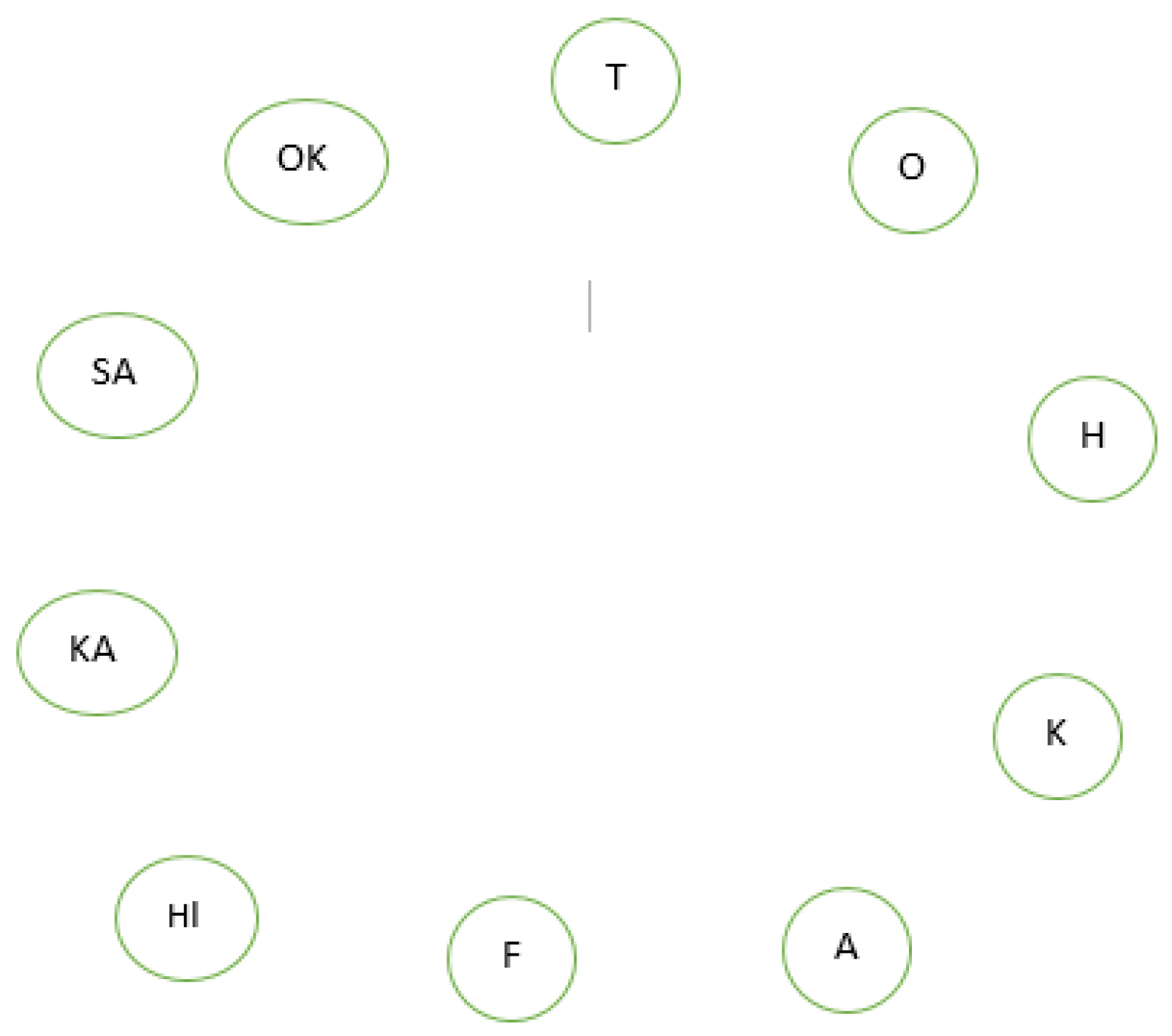
• Situation (i): Building Earthquake-Resistant Facilities in 10 Chosen Regions
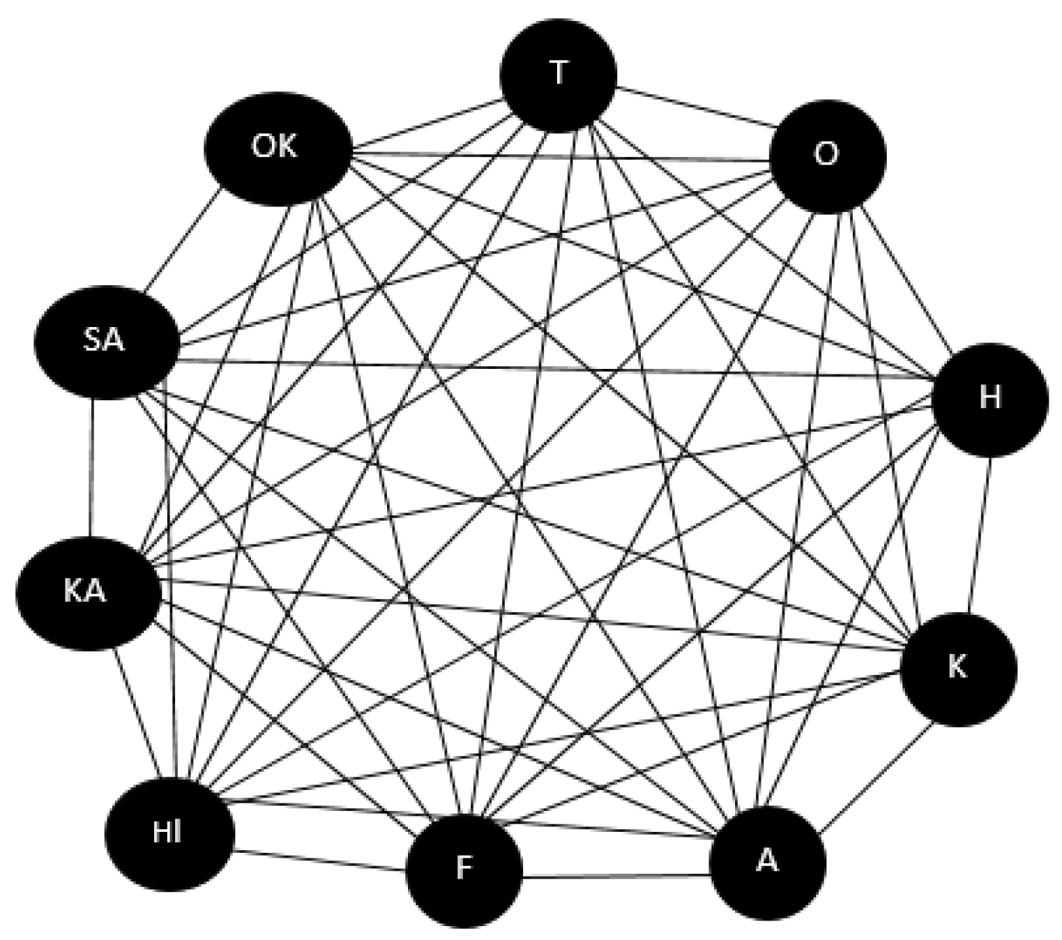
• Situation (ii): Building an intermediary earthquake response center between any two chosen Regions.

Situation 1: Given a set of Japanese regions where the team wishes to establish an earthquake response center, denoted as the vertex set $S=\left\{Tokyo\left(T\right),Osaka\left(O\right),Hokkaido\left(H\right),Kyoto\left(K\right),\right.\left.Aichi\left(A\right),Fukuoka\left(F\right),Hiroshima\left(HI\right),Kanagawa\left(KA\right),Saitama\left(SA\right),Okinawa\left(OK\right)\right\}$ The team assesses the opinions of experts on the necessity of starting an earthquake response center in each region. Tokyo has strong earthquake preparedness, with 80% agreeing, 20% having a moderate opinion, and 10% disagreeing. The model for Tokyo may be represented as $(T:0.8,0.2,0.1)$. Experts are uncertain about the earthquake preparedness in Osaka, with 50% agreeing, 40% having a moderate opinion, and 30% disagreeing. The model for Osaka may be represented as $<O:0.5,0.4,0.3>$. Experts strongly agree that Hokkaido has excellent earthquake preparedness, with 90% agreeing, 10% having a moderate opinion, and 5% disagreeing. The model for Hokkaido may be represented as $<H:0.9,0.1,0.05>$. Kyoto is considered moderately prepared for earthquakes, with 60% agreeing, 30% having a moderate opinion, and 20% disagreeing. The model for Kyoto may be represented as $<K:0.6,0.3,0.2>$. Aichi is perceived as well-prepared for earthquakes, with 70% agreeing, 20% having a moderate opinion, and 10% disagreeing. The model for Aichi may be represented as $<A:0.7,0.2,0.1>$. Fukuoka has mixed opinions, with 40% agreeing, 50% having a moderate opinion, and 40% disagreeing. The model for Fukuoka may be represented as $<F:0.4,0.5,0.4>$. Hiroshima has strong earthquake preparedness, with 80% agreeing, 15% having a moderate opinion, and 5% disagreeing. The model for Hiroshima may be represented as $<HI:0.8,0.15,0.05>$. Kanagawa is considered moderately prepared, with 60% agreeing, 30% having a moderate opinion, and 20% disagreeing. The model for Kanagawa may be represented as $<KA:0.6,0.3,0.2>$. Experts strongly agree that Saitama has excellent earthquake preparedness, with 90% agreeing, 10% having a moderate opinion, and 5% disagreeing. The model for Saitama may be represented as $<SA:0.9,0.1,0.05>$. Okinawa is perceived as well-prepared for earthquakes, with 70% agreeing, 20% having a moderate opinion, and 10% disagreeing. The model for Okinawa may be represented as $<OK:0.7,0.2,0.1>$ we denote this model as

$$A=\left\{\begin{array}{c}\langle T:0.8,0.2,0.1\rangle \hfill \\ <O:0.5,0.4,0.3>\hfill \\ <H:0.9,0.1,0.05>\hfill \\ <K:0.6,0.3,0.2>\hfill \\ <A:0.7,0.2,0.1>\hfill \\ <F:0.4,0.5,0.4>\hfill \\ <HI:0.8,0.15,0.05>\hfill \\ <KA:0.6,0.3,0.2>\hfill \\ <SA:0.9,0.1,0.05>\hfill \\ <OK:0.7,0.2,0.1>\hfill \end{array}\right.$$

vertex true and ambiguity membership indicates the good aspects of a certain parameter for a given location, whereas vertex false membership indicates its negative aspects. Now that we have found ultimate values, we must

$$\begin{gathered} \left|T\right|=(0.8,0.2,0.1),\left|O\right|=(0.5,0.4,0.3), \\ \left|H\right|=(0.9,0.1,0.05),\left|K\right|=(0.6,0.3,0.2), \\ \left|A\right|=(0.7,0.2,0.1),\left|F\right|=(0.4,0.5,0.4), \\ \left|HI\right|=(0.8,0.15,0.05),\left|KA\right|=(0.6,0.3,0.2), \\ \left|SA\right|=(0.9,0.1,0.05),\left|OK\right|=(0.7,0.2,0.1). \end{gathered}$$

We determine the score function of the absolute values of $T,O,H,K,A,F,HI,KA,SA,$, and $OK$ in order to establish an earthquake response center. Consequently, we have

$$\begin{gathered} S\left(T\right)=(0.8-0.2-0.1)=0.5, \\ S\left(O\right)=(0.5-0.4-0.3)=-0.2, \\ \mathbf{S}\left(\mathbf{H}\right)=(\mathbf{0}.\mathbf{9}-\mathbf{0}.\mathbf{1}-\mathbf{0}.\mathbf{05})=\mathbf{0}.\mathbf{75} \\ S\left(K\right)=(0.6-0.3-0.2)=0.1 \\ S\left(A\right)=(0.7-0.2-0.1)=0.4 \\ S\left(F\right)=(0.4-0.5-0.4)=-0.5 \\ \mathbf{S}\left(\mathbf{HI}\right)=(\mathbf{0}.\mathbf{8}-\mathbf{0}.\mathbf{15}-\mathbf{0}.\mathbf{05})=\mathbf{0}.\mathbf{6}, \\ S\left(KA\right)=(0.6-0.3-0.2)=0.1 \\ S\left(SA\right)=(0.9-0.1-0.05)=0.45 \\ S\left(OK\right)=(0.7-0.2-0.1)=0.4 \end{gathered}$$

The maximum score value of H and $HI$ is 0.75 and 0.6, thus $H>HI$ is the largest value and therefore more suitable for establishing an earthquake response center. The neutrosophic graph with no edges is shown in Figure 9.

For Issue 2, we now go forward in the manner of, if we establish an earthquake response center fixed between places $T\&O$, it will represent the edge $\langle T-O\rangle$ of the vertex T and O. To find the model of $\langle T-O\rangle$, we use Definition 2 and find that $\langle T-O:0.5,0.2,0.3\rangle$. Similarly, the other edges are presented in

Table 2. Absolute values of the edges for Figure 10.

Locations	Neutrosophic Membership Values	Locations	Neutrosophic Membership Values
|T-O|	(0.5, 0.2, 0.3)	|T-H|	(0.8, 0.1, 0.1)
|T-K|	(0.6, 0.2, 0.2)	|T-A|	(0.7, 0.2, 0.1
|T-F|	(0.4, 0.2, 0.4)	|T-HI|	(0.5, 0.15, 0.5)
|T-KA|	(0.6, 0.2, 0.2)	|T-SA|	(0.8, 0.1, 0.1)
|T-OK|	(0.7, 0.2, 0.1)	|O-H|	(0.5, 0.1, 0.3)
|O-K|	(0.5, 0.3, 0.3)	|O-A|	(0.5, 0.2, 0.3)
|O-F|	(0.4, 0.4, 0.4)	|O-HI|	(0.5, 0.15, 0.3)
|O-KA|	(0.5, 0.3, 0.3)	|O-SA|	(0.5, 0.1, 0.3)
|O-OK|	(0.5, 0.2, 0.3)	|H-K|	(0.6, 0.1, 0.2)
|H-A|	(0.4, 0.1, 0.5)	|H-F|	(0.4, 0.1, 0.8)
|H-HI|	(0.5, 0.1, 0.05)	|H-KA|	(0.6, 0.1, 0.2)
|H-SA|	(0.9, 0.1, 0.05)	|H-OK|	(0.7, 0.1, 0.1)
|K-A|	(0.6, 0.2, 0.2)	|K-F|	(0.4, 0.2, 0.4)
|K-HI|	(0.5, 0.15, 0.2)	|K-KA|	(0.6, 0.3, 0.2)
|K-SA|	(0.6, 0.1, 0.2)	|K-OK|	(0.6, 0.2, 0.2)
|A-F|	(0.4, 0.2, 0.4)	|A-HI|	(0.5, 0.15, 0.4)
|A-KA|	(0.6, 0.2, 0.2)	|A-SA|	(0.7, 0.1, 0.1)
|A-OK|	(0.7,0.2, 0.1)	|F-HI|	(0.4, 0.15, 0.5)
|F-KA|	(0.4, 0.3, 0.4)	|F-SA|	(0.4, 0.1, 0.4)
|F-OK|	(0.4, 0.2, 0.4)	|HI-KA|	(0.5, 0.1, 0.5)
|HI-SA|	(0.5, 0.1, 0.05)	|HI-OK|	(0.5, 0.1, 0.05)
|KA-SA|	(0.6, 0.1, 0.05)	|KA-OK|	(0.6, 0.2, 0.2)
|SA-OK|	(0.7, 0.1, 0.1)	-	-

We determine the score function of the edge absolute values in order to choose and establish an earthquake response center. The score function of the edges is defined as:

$S(\stackrel{`}{\omega },\stackrel{`}{\upsilon })$ = (Absolute values of $T^R$− Absolute values of $I^N$− Absolute values of $F^S$)

$S(H,SA)$ is the largest value and therefore more suitable for establishing an earthquake response center. In Figure 11, there is a graphical representation of

Table 3. Score function of the edge absolute values.

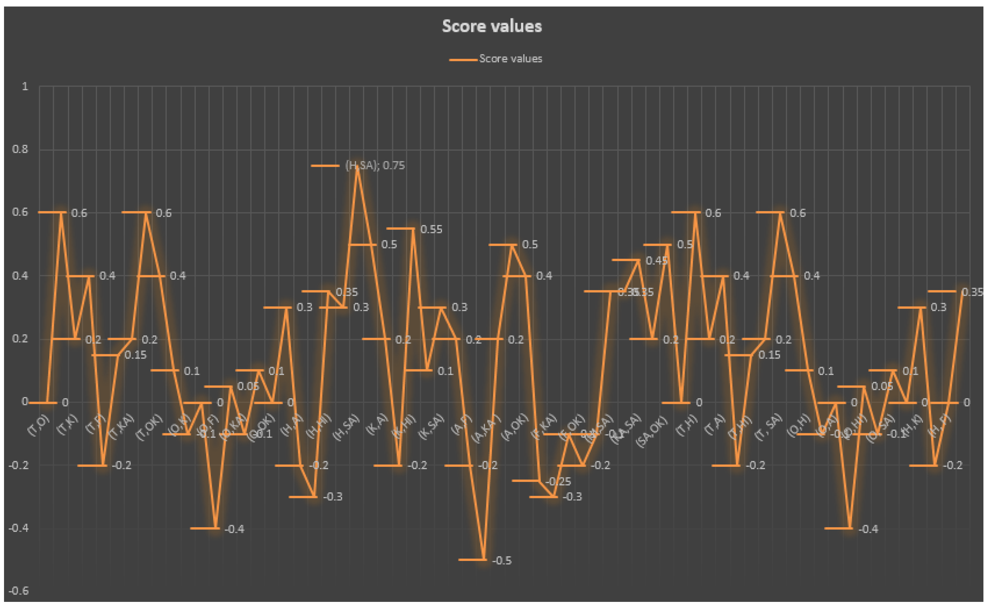
Edges	Score Functions	Edges	Score Functions
S(T-O)	0	S(T,H)	0.6
S(T-K)	0.2	S(T,A)	0.4
S(T-F)	−0.2	S(T,HI)	0.15
S(T-KA)	0.2	S(T,SA)	0.6
S(T-OK)	0.4	S (O,H)	0.1
S(O-K)	−0.1	S(O,A)	0
S(O-F)	−0.4	S(O,HI)	0.05
S(O-KA)	−0.1	S(O,SA)	0.1
S(O-OK)	0	S(H,K)	0.3
S(H-A)	−0.2	S(H,F)	−0.3
(H-HI)	0.35	S(H,KA)	0.3
S(H-SA)	0.75	S(H,OK)	0.5
S(K-A)	0.2	S(K,F)	−0.2
S(K-HI)	0.55	S(K,KA)	0.1
S(K-SA)	0.3	S(K,OK)	0.2
S(A-F)	−0.2	S(A,HI)	−0.5
S(A-KA)	0.2	S(A,SA)	0.5
S(A-OK)	0.4	S(F,HI)	−0.25
S(F-KA)	−0.3	S(F,SA)	0.1
S(F-OK)	−0.2	S(HI,KA)	−0.1
S(HI-SA)	0.35	S(HI,OK)	0.35
S(KA-SA)	0.45	S(KA,OK)	0.2
S(SA-OK)	0.5	–	–

; it is clear that the suitable location to establish an earthquake response center is $S(H,SA)$.

5.1. Comparative Analysis

In this section, we compared various score function formulae, and its corresponding values are presented.

• In [38], Jian-qiang Wang et al. Score function formula and value are given by
  $S\left(V\right)=\frac{{\mu }_{T^R}+1-{\mu }_{I^N}+1-{\mu }_{F^S}}{3}=0.91$
• In [39], Rıdvan Şahin, Score function formula and value are given by
  $S\left(V\right)=\frac{1+T^R-2I^N+1-F^S}{2}=0.825$
• In [40], Said Broumi al. Score function formula and value given by
  $S\left(V\right)=\frac{T^R+I^N+1-F^S}{3}=0.95.$

Hence for all existing models, the value of $(H-SA)$ has been common. But in our proposed model it mainly focused on the absolute value of score functions, which is very easy to calculate for any data, which makes better decisions.

5.2. Connections and Discussions of the Results

By investigating the relationship between neutrosophic graph theory and its implementation in Japan’s earthquake response centers, we can make progress in theoretical knowledge and real-world applications that improve preparedness and reaction times for disasters.

6. Conclusions

In this paper, we have discussed basic operations on neutrosophic graphs such as product, union, composition, … etc. The neutrosophic graph has been used to establish the earthquake prediction center at various locations in the country of Japan. Vertices involved in a neutrosophic graph are more useful to make better decisions. The mathematical foundation of neutrosophic graph theory tends to identify suitable locations in Japan to overcome disasters during earthquakes.

Future Work:

• Certain types of super hyper $\aleph G$s.
• Dominating energy in hyper $\aleph G$s
• Maximal product of super hyper $\aleph Gs$ and its real time applications.
• Operation of super hyper $\aleph G$.

References

- Zadeh, L.A. Fuzzy sets. Inf. Control 1965, 8, 338–353. [Google Scholar] [CrossRef]
- Atanassov Krassimir, T. Intuitionistic fuzzy sets. In Intuitionistic Fuzzy Sets; Springer: New York, NY, USA, 2019; pp. 1–137. [Google Scholar]
- Smarandache, F. A unifying field in logics: Neutrosophic logic. In Philosophy; American Research Press: New York, NY, USA, 1999; pp. 1–141. [Google Scholar]
- Smarandache, F. A Unifying Field in Logics: Neutrosophic Logic. Neutrosophy, Neutrosophic Set, Neutrosophic Probability and Statistics, 6th ed.; InfoLearnQuest: Philadelphia, PA, USA, 2007. [Google Scholar]
- Borzooei, R.A.; Rashmanlou, H.; Samanta, S.; Pal, M. Regularity of vague graphs. J. Intell. Fuzzy Syst. 2016, 30, 3681–3689. [Google Scholar] [CrossRef]
- Waseem, N.; Dudek, W.A. Certain types of edge m-polar fuzzy graphs. Iran. J. Fuzzy Syst. 2017, 14, 27–50. [Google Scholar]
- Ghorai, G.; Pal, M. Certain types of product bipolar fuzzy graphs. Int. J. Appl. Comput. Math. 2017, 3, 605–619. [Google Scholar] [CrossRef]
- Naz, S.; Rashmanlou, H.; Malik, M.A. Operations on single valued ℵGs with application. J. Intell. Fuzzy Syst. 2017, 32, 2137–2151. [Google Scholar] [CrossRef]
- Sahoo, S.; Pal, M. Different types of products on intuitionistic fuzzy graphs. Pac. Sci. Rev. A Nat. Sci. Eng. 2015, 17, 87–96. [Google Scholar] [CrossRef]
- Yang, H.-L.; Guo, Z.-L.; She, Y.; Liao, X. On single valued neutrosophic relations. J. Intell. Fuzzy Syst. 2006, 30, 1045–1056. [Google Scholar] [CrossRef]
- Ye, J. Single-valued neutrosophic minimum spanning tree and its clustering method. J. Intell. Syst. 2014, 23, 311–324. [Google Scholar] [CrossRef]
- Shannon, A.; Atanassov, K. On a generalization of intuitionistic fuzzy graphs. NIFS 2006, 12, 24–29. [Google Scholar]
- Parvathi, R.; Karunambigai, M.G. Intuitionistic fuzzy graphs. In Computational Intelligence, Theory and Applications; Springer: New York, NY, USA, 2006; pp. 139–150. [Google Scholar]
- Parvathi, R.; Karunambigai, M.G.; Atanassov, K.T. Operations on intuitionistic fuzzy graphs. In Proceedings of the 2009 IEEE International Conference on Fuzzy Systems, Jeju, Republic of Korea, 20–24 August 2009; pp. 1396–1401. [Google Scholar]
- Parvathi, R.; Thamizhendhi, G. Domination in intuitionistic fuzzy graphs. Notes Intuit Fuzzy Sets 2010, 16, 39–49. [Google Scholar]
- Rashmanlou, H.; Borzooei, R.A.; Samanta, S.; Pal, M. Properties of interval valued intuitionistic (s, t)–fuzzy graphs. Pac. Sci. Rev. A Nat. Sci. Eng. 2016, 18, 30–37. [Google Scholar] [CrossRef]
- Rashmanlou, H.; Samanta, S.; Pal, M.; Borzooei, R.A. Bipolar fuzzy graphs with categorical properties. Int. J. Comput. Intell. Syst. 2015, 8, 808–818. [Google Scholar] [CrossRef]
- Rashmanlou, H.; Samanta, S.; Pal, M.; Borzooei, R.A. Intuitionistic fuzzy graphs with categorical properties. Fuzzy Inf. Eng. 2015, 7, 317–334. [Google Scholar] [CrossRef]
- Smarandache, F. Extension of hypergraph to n-superhypergraph and to plithogenic n-superhypergraph, and extension of hyperalgebra to n-ary hyperalgebra. Neutrosophic Sets Syst. 2020, 33, 290–296. [Google Scholar]
- Akram, M. Certain bipolar neutrosophic competition graphs. J. Indones. Math. Soc. 2017, 24, 1–25. [Google Scholar] [CrossRef]
- Akram, M.; Akmal, R. Operations on intuitionistic fuzzy graph structures. Fuzzy Inf. Eng. 2016, 8, 389–410. [Google Scholar] [CrossRef]
- Akram, M.; Dar, J.M.; Naz, S. Certain graphs under pythagorean fuzzy environment. Complex Intell. Syst. 2019, 5, 127–144. [Google Scholar] [CrossRef]
- Akram, M.; Habib, A.; Ilyas, F.; Dar, J.M. Specific types of pythagorean fuzzy graphs and application to decision-making. Math. Comput. Appl. 2018, 23, 42. [Google Scholar] [CrossRef]
- Akram, M.; Naz, S. Energy of pythagorean fuzzy graphs with applications. Mathematics 2018, 6, 136. [Google Scholar] [CrossRef]
- Akram, M.; Siddique, S. Neutrosophic competition graphs with applications. J. Intell. Fuzzy Syst. 2017, 33, 921–935. [Google Scholar] [CrossRef]
- Karaaslan, F.; Hayat, K.; Jana, C. The Determinant and Adjoint of an Interval-Valued Neutrosophic Matrix. In Neutrosophic Operational Research; Smarandache, F., Abdel-Basset, M., Eds.; Springer: Cham, Switzerland, 2021. [Google Scholar]
- Hayat, K.; Cao, B.-Y.; Ali, M.I.; Karaaslan, F.; Qin, Z. Characterizations of Certain Types of Type 2 Soft Graphs. Discret. Dyn. Nat. Soc. 2018, 2018, 8535703. [Google Scholar] [CrossRef]
- Karaaslan, F.; Hayat, K. Some new operations on single-valued neutrosophic matrices and their applications in multi-criteria group decision making. Appl. Intell. 2018, 48, 4594–4614. [Google Scholar] [CrossRef]
- Majeed, A.S.; Arif, N.E. Topological indices of certain neutrosophic graphs. Aip Conf. Proc. 2023, 2845, 060024. [Google Scholar]
- Kaviyarasu, M. On r-Edge Regular Neutrosophic Graphs. Neutrosophic Sets Syst. 2023, 53, 239–250. [Google Scholar]
- AL-Omeri, W.F.; Kaviyarasu, M.; Rajeshwari, M. Identifying Internet Streaming Services using Max Product of Complement in Neutrosophic Graphs. Int. J. Neutrosophic Sci. 2024, 3, 257–272. [Google Scholar] [CrossRef]
- Yaqoob, N.; Gulistan, M.; Kadry, S.; Wahab, H.A. Complex Intuitionistic Fuzzy Graphs with Application in Cellular Network Provider Companies. Mathematics 2019, 7, 35. [Google Scholar] [CrossRef]
- Mahapatra, R.; Samanta, S.; Pal, M.; Xin, Q. Link Prediction in Social Networks by Neutrosophic Graph. Int. J. Comput. Intell. Syst. 2020, 13, 1699–1713. [Google Scholar] [CrossRef]
- Srisarkun, V.; Jittawiriyanukoon, C. An approximation of balanced score in neutrosophic graphs with weak edge weights. Int. J. Electr. Comput. Eng. 2021, 11, 5286–5291. [Google Scholar] [CrossRef]
- Mahapatra, R.; Samanta, S.; Pal, M. Edge Colouring of Neutrosophic Graphs and Its Application in Detection of Phishing Website. Discret. Dyn. Nat. Soc. 2022, 2022, 1149724. [Google Scholar] [CrossRef]
- Quek, S.G.; Selvachandran, G.; Ajay, D.; Chellamani, P.; Taniar, D.; Fujita, H.; Duong, P.; Son, L.H.; Giang, N.L. New concepts of pentapartitioned neutrosophic graphs and applications for determining safest paths and towns in response to COVID-19. Comp. Appl. Math. 2022, 41, 151. [Google Scholar] [CrossRef]
- Alqahtani, M.; Kaviyarasu, M.; Al-Masarwah, A.; Rajeshwari, M. Application of Complex Neutrosophic Graphs in Hospital Infrastructure Design. Mathematics 2024, 12, 719. [Google Scholar] [CrossRef]
- Wang, J.-q.; Wang, J.; Chen, Q.-h.; Zhang, H.-y.; Chen, X.-h. An outranking approach for multi-criteria decision-making with hesitant fuzzy linguistic term sets. Inf. Sci. 2014, 280, 338–351. [Google Scholar] [CrossRef]
- Şahin, R. Multi-criteria neutrosophic decision making method based on score and accuracy functions under neutrosophic environment. Inf. Sci. 2014, 280, 338–351. [Google Scholar]
- Broumi, S.; Sundareswaran, R.; Shanmugapriya, M.; Bakali, A.; Talea, M. Theory and Applications of Fermatean Neutrosophic Graphs. Neutrosophic Sets Syst. 2002, 50, 248–286. [Google Scholar]