Abstract
The economic friction and political conflicts between some countries and regions have made multinational corporations increasingly focus on the reliability and credibility of manufacturing supply chains. In view of the impact of poor manufacturing entity reliability and service reputation on the new-era manufacturing industry, the time-varying reliability and time-varying credibility of cloud manufacturing (CMfg) services were studied from the perspective of combining nature and society. Taking time-varying reliability, time-varying credibility, composition complexity, composition synergy, execution time, and execution cost as objective functions, a new six-dimension comprehensive evaluation model of service quality was constructed. To solve the optimization problem, this study proposes an improved chaos sparrow search algorithm (ICSSA), where the Bernoulli chaotic mapping formula was introduced to improve the basic sparrow search algorithm (BSSA), and the position calculation formulas of the explorer sparrow and the scouter sparrow were enhanced. The Bernoulli chaotic operator changed the symmetry of the BSSA, increased the uncertainty and randomness of the explorer sparrow position in the new algorithm, and affected the position update and movement strategies of the follower and scouter sparrows. The asymmetric chaotic characteristic brought better global search ability and optimization performance to the ICSSA. The comprehensive performance of the service composition (SvcComp) scheme was evaluated by calculating weighted relative deviation based on six evaluation elements. The WFG and DTLZ series test functions were selected, and the inverse generation distance (IGD) index and hyper volume (HV) index were used to compare and evaluate the convergence and diversity of the ICSSA, BSSA, PSO, SGA, and NSGA-III algorithms through simulation analysis experiments. The test results indicated that the ICSSA outperforms the BSSA, PSO, SGA, and NSGA-III in the vast majority of testing issues. Finally, taking disinfection robot manufacturing tasks as an example, the effectiveness of the proposed CMfg SvcComp optimization model and the ICSSA were verified. The case study results showed that the proposed ICSSA had faster convergence speed and better comprehensive performance for the CMfg SvcComp optimization problem compared with the BSSA, PSO, SGA, and NSGA-III.
1. Introduction
Over the past half-century, the global economy has demonstrated that openness, collaboration, and innovation hold the key to advancing manufacturing and economic growth. The disruptive influence of volatile factors, such as trade frictions, has significantly impacted the open and collaborative landscape, thereby slowing the pace of development in the global manufacturing industry. Currently, businesses are placing a heightened emphasis on the reliability of manufacturing supply chains [1]. Consequently, numerous nations have prioritized the establishment of highly trustworthy and dependable manufacturing supply chains and services at the national decision-making level. Cloud manufacturing (CMfg), a service-centered manufacturing approach, aligns with the evolving needs of the manufacturing industry in the contemporary era [2]. It offers a viable solution to address the challenges posed by diverse consumer demands and shortened product market cycles [3]. The CMfg service platform virtualizes and offers manufacturing resources and capabilities, enabling centralized oversight of distributed manufacturing assets and tailored services to a diverse user community [4]. In the intricate and dynamically evolving international landscape, an analysis of time-varying reliability and credibility offers enhanced insights for CMfg service selection and user decision-making.
The construction of the CMfg service composition (SvcComp) model, along with its associated solution algorithm, serves as a crucial element in determining the effectiveness of the optimal SvcComp plan. Furthermore, it significantly impacts the efficiency and profitability of CMfg resources. The optimization of CMfg SvcComp is characterized by its multi-objective nature, nonlinearity, and inherent uncertainty. Consequently, numerous scholars are devoting themselves to addressing the intricate NP problem [5]. Scholars primarily focus on production cost, execution time, and profit as key optimization parameters in their exploration of SvcComp modeling and optimization algorithms. However, they infrequently take into account the influence of non-functional service quality factors, including service reliability, reputation, and composition synergy, on the overall SvcComp. The execution of CMfg entails a collaborative effort involving various distributed manufacturing resources. Notably, each CMfg service execution agent operates within a specific natural and social context, deviating from the idealized perception of a “rigid body”. Within the CMfg process, diverse CMfg services engage in data exchange, information transmission, and material transportation. The interactions give rise to constraints, collaborations, and competitions that persist throughout the entire manufacturing lifecycle. The interplay among services and tasks, among services themselves, and with agents occupies a vital position in determining the effectiveness and efficiency of SvcComp in executing manufacturing tasks. Instances such as war friction and the Red Sea crisis highlight the significance of manufacturing enterprises being deeply embedded in the global industrial chain to leverage both service credibility and reliability alongside manufacturing cost and time as key metrics for assessing CMfg service quality. This approach ensures the provision of more credible, reliable, and efficient services to users. In the intricate and dynamic international landscape, the time-varying nature of reliability and credibility significantly influences the overall performance and service selection within CMfg SvcComp. The CMfg environment necessitates the collaborative efforts of various executing agents, encompassing service providers, operators, customers, and more. The collaboration is influenced by both natural and social factors. The reliability of CMfg services, the degree of collaboration among services during the manufacturing process, the credibility of these services, and the complexity of the SvcComp all play crucial roles in the successful accomplishment of manufacturing endeavors. Therefore, while adhering to the constraints of delivery time and manufacturing cost, it is imperative to optimize CMfg SvcComp by prioritizing parameters such as service reliability, composition synergy, service credibility, and composition complexity.
The fundamental principle of SvcComp dictates that all manufacturing tasks stemming from the decomposition of manufacturing demands must be assigned to either a single cloud service or multiple cloud services for execution. The optimal CMfg SvcComp scheme should exhibit optimal overall performance, encompassing maximum service reliability, composition synergy, and service credibility, while minimizing composition complexity, delivery time, and manufacturing cost. The key contributions of this work are outlined as follows: (1) an improved chaos sparrow search algorithm tailored for CMfg SvcComp is introduced; (2) a CMfg SvcComp optimization model, incorporating factors such as time-varying reliability, time-varying credibility, and composition complexity, is developed; (3) an illustrative application example is presented to demonstrate the effectiveness of the proposed mathematical model and optimization algorithm.
The rest of this paper is structured as follows: Section 2 conducts a comprehensive analysis of domestic and international research on service reliability, service credibility, CMfg SvcComp, and its associated optimization algorithms. Section 3 defines and outlines the calculation methods for time-varying reliability, composition synergy, time-varying credibility, composition complexity, execution time, and execution cost. Section 4 introduces an improved algorithm, while Section 5 validates the effectiveness of the proposed method through a detailed analysis of practical applications. Finally, Section 6 concludes this paper and underscores the significance of the work.
2. Related Work
In recent years, various scholars have delved into the modeling and optimization of cloud SvcComp, leveraging techniques such as genetic algorithms and particle swarm optimization. By synthesizing the prior research efforts of these scholars, we meticulously selected the most pertinent studies and categorized the existing research into three distinct groups.
The first group studied service reliability and service credibility. In the research of service credibility, Qiu-yun Zhao et al. [6] put forward a support mechanism for credibility in CMfg services, which hinged on a classified approach to QoS, described the environment information and the level of QoS in the manufacturing cloud service model, and constructed an adaptive control logic algorithm to adjust the QoS level. Tooba Aamir et al. proposed a credibility model of social sensor cloud service based on user’s position and credibility. It used comments and metadata of cloud service to collect the trust rate of the service and the credibility of the users’ comments [7]. R. Tang et al. proposed an algorithm of cloud media resource allocation based on credibility, which allocated cloud media resources based on total credibility to obtain the optimal allocation sequence of higher allocation efficiency and service quality [8]. Suzhen Wang et al. proposed a trust management model based on credibility, which could distinguish trust feedback and detect malicious trust feedback of attackers [9]. Lie Qu et al. proposed a new model for evaluating the reliability of users, which provided subjective evaluation by ordinary cloud consumers and objective evaluation by professional testers for cloud services, and could resist user collusion [10]. Xiaogang Cai et al. proposed a method of evaluating and modifying reputation based on node credibility [11]. By calculating the reputation of each node and modifying the reputation value, the accuracy of reputation results was improved, and an incentive mechanism was introduced to improve the enthusiasm of cloud user node evaluation. Khamdi Mubarok et al. proposed a hierarchical model for reliability assessment, specifically designed to evaluate the dependability of manufacturing services. In this model, enterprise manufacturing resources were categorized into three distinct levels, component, machine, and system, enabling a comprehensive reliability evaluation [12]. Combining explicit text information with rating information and implicit context information, Jian Liu et al. determined task similarity and employed a clustering-based approach to identify cohorts of users sharing similar characteristics [13]. They further devised a trust perception methodology that merged both local and global trust metrics, reconstructing the trust network among clustered users. Additionally, they introduced a prediction and recommendation strategy for service quality, grounded in clustering and trust perception principles. Shikai Jing et al. put forward an SvcComp approach for CMfg, leveraging discrete particle swarm optimization with a focus on execution reliability [14]. The probability density function was used to describe the service reliability, and the CMfg SvcComp workflow model was dynamically generated based on the service model library. Chen Jiang et al. proposed a real-time estimation error-guided sampling method for time-varying reliability analysis, used Kriging prediction mean and variance to calculate the probability of error classification, obtained the total number of error classification points, and calculated the estimation error of fault probability based on confidence intervals [15]. Junejo A.K. et al. studied a cloud service trust computing framework that calculates credibility by aggregating multidimensional evidence of quality of service and quality of experience [16]. The approach integrated the principles of complex networks to provide a comprehensive assessment of accounting cloud service reliability. Zhiqiang Wan et al. analyzed the problem of the monotonic degradation of materials and time-varying reliability evaluation of parametric random loads, and proposed a new method combining the probability density evolution method and probability measure change [17]. Hua-Ming Qian et al. introduced a decoupling technique for single-loop processes, alongside a double-closed-loop Kriging model, specifically tailored for time-varying reliability analysis [18]. Hong-Shuang Li et al. proposed a high-dimensional time-varying reliability analysis method that incorporated random sampling and treated random processes as inputs [19]. The time-varying reliability analysis was transformed into the reliability problem of series systems with multiple responses. M.H. Ping et al. proposed a time-varying extreme event evolution method and simulated the time evolution process of extreme events by the time-dependent polynomial chaotic expansion method [20]. Monte Carlo simulation was used to sample the standard normal variables, and the time-varying reliability of the failure threshold was obtained.
The second group delved into the intricacies of manufacturing task decomposition and SvcComp. Mingzhou Liu et al. introduced a CMfg task decomposition algorithm that employed sequential task decomposition, leveraging a recursive decomposition approach to enhance the optimization of decomposed tasks [21]. Aijun Liu et al. developed a quantitative analysis technique for task granularity, which assessed the granularity of complex product collaborative workflows within integrated manufacturing systems [22]. The method served as a guide for coarse-grained task decomposition and the reorganization of sub-tasks with low cohesion coefficients. Shuping Yi et al. proposed a task decomposition optimization strategy grounded in clustering algorithms [23]. By reconstructing decomposed sub-tasks using clustering techniques, they achieved optimal task decomposition and offered a solution to the disjoint issue that arose in manufacturing task decomposition and resource allocation. Katz Dmitriy et al. investigated two variations of the classic job interval scheduling problem, focusing on the flexible allocation of reusable resources among competing job intervals [24]. J. Thekinen et al. examined the objectives and preferences of service seekers and providers in cloud-based design and manufacturing [25]. They further evaluated the suitability of various matching mechanisms in the context of cloud design and manufacturing. Octavian Morariu et al. explored service-oriented approaches for enhancing resource allocation in a private cloud environment [26]. They introduced an extended queued resource allocation bus architecture that incorporated the computation of alternative schedules for optimized resource utilization. Yang-Kuei Lin et al. proposed a resource-constrained project scheduling method based on a genetic algorithm, which integrated novel concepts like enhancement and local search, addressing the challenges associated with computing resource allocation in cloud computing systems [27]. Buyun Sheng et al. delved into the complexities of the matching process between an intelligent matching engine and CMfg services, emphasizing their diversity, heterogeneity, and multi-constraints [28]. They developed an intelligent search engine tailored for small and medium-sized enterprises’ CMfg services, leveraging service ontology language to facilitate swift and efficient cloud search matching. Fei Tao et al. introduced a supply–demand matching simulator specifically for manufacturing services, outlining a simulator architecture grounded in hyper-networks [29]. Jinhui Zhao et al. proposed a bilateral matching model for cloud services, emphasizing the role of quality of service in the matching process [30]. It calculated satisfaction degree by the variable fuzzy identification method. Yuqian Lu et al. delved into the realm of knowledge-based SvcComp and adaptive resource planning within the CMfg environment [31]. They constructed an integrated network environment that could swiftly allocate resources for specific service requests, leveraging governance strategies, resource access mechanisms, and availability information. Jorick Lartigau et al. recognized the commonalities among cloud services, including QoS parameters, but broadened their focus to include the physical locale of manufacturing resources [32]. They introduced a methodology that combines QoS evaluation with geo-perspective correlation across cloud services, enabling a comprehensive analysis of transportation impacts. Marcos A. Pisching et al. studied the characteristics and major challenges of industrial 4.0 SvcComp based on CMfg [33]. Yan Xiao et al. introduced a decision-making framework for manufacturing service resource matching, emphasizing the fusion of multidimensional information [34]. Leveraging the integration of various information data sources from CMfg resources, they categorized the significance of manufacturing service tasks using information entropy and rough set theory. Hamed Bouzary et al. proposed a hybrid algorithm which combines the grey wolf optimization algorithm and the genetic algorithm [35]. The embedded crossover and mutation operators enabled the continuous structure of the grey wolf algorithm to adapt to combinatorial problems such as SvcComp optimization selection. Mohammad Moein Fazeli et al. proposed an integrated optimization method for choosing the best composition of services to execute customer requests [36].
The third group focused on service quality evaluation and optimization algorithms. K. He et al. [37] outlined selection criteria for CMfg service providers within the CMfg system and developed a comprehensive evaluation index system incorporating a scalable quantitative model. The triangular fuzzy number algorithm was used to calculate the similarity and demand expectation between service providers, and the comprehensive performance ranking of service quality was obtained. Shangguang Wang et al. proposed an accurate evaluation method of cloud service quality [38]. According to the preferences of cloud users, a fuzzy comprehensive decision method was used to evaluate cloud service providers. Xinggang Wang et al. proposed a task evaluation index system for 3D printing orders for innovative new product development in a CMfg environment [39]. The evaluation index included eight dimensions: execution time, service quality, matching, reliability, flexibility, cost, fault tolerance, and satisfaction. Yuan Ye et al. proposed an evaluation system of e-government service quality for telecom operators and evaluated the service quality based on network factors, service process factors, collaboration factors, and resource allocation factors [40]. Yanjuan H et al. delved into the challenges of manufacturer scheduling within the CMfg environment [41]. They thoroughly analyzed the influencing factors of manufacturer resource scheduling, encompassing task load, task reliability, manufacturing efficiency, resource abundance, and IoT matching. Utilizing a chaotic optimization algorithm, they addressed the objective function, successfully realizing manufacturer scheduling across various tasks. Yongxiang Li et al. introduced a CMfg SvcComp optimization approach leveraging cloud entropy-enhanced genetic algorithms [42]. They outlined methods for computing service matching, composition coordination, and cloud entropy, establishing a multi-objective optimization model for CMfg SvcComp. Wenjun Xu et al. proposed an enhanced Pareto-based discrete bees algorithm, aiming to select optimal services from a vast array of CMfg offerings, combining them to create new, high-performance services [43]. Onaizah N A and Aljanabi R M presented a novel approach, the chaotic African vulture optimization algorithm integrated with a deep learning-driven solid waste classification system, termed CAVOA-DLSWC. Its objective was to automatically identify waste objects and categorize them into distinct groups utilizing advanced deep learning models [44]. M. Tavana et al. introduced a discrete cuckoo optimization algorithm, leveraging group technology for seamless resource allocation integration [45]. Fateh Seghir et al. proposed a hybrid genetic algorithm specifically tailored to address the cloud SvcComp challenge, with a focus on quality of service perception [46]. It combined the genetic algorithm and drosophila optimization to search the evolutionary process. Xianmin Wei et al. studied the optimal resource allocation for CMfg. Utilizing a four-dimensional objective function encompassing time, cost, quality of service, and load balancing, an ant colony algorithm was employed to discover the optimal solution [47]. Yi Que et al. introduced a user-centered manufacturing model for the manufacturer cloud, developing a comprehensive mathematical evaluation framework that encompassed four crucial service quality perception metrics: time, reliability, cost, and capability [48]. They further proposed an information entropy-based immune genetic algorithm to enhance the selection of core manufacturing SvcComps. Hui Jiang et al. developed a multi-objective genetic algorithm grounded in non-dominated sorting techniques to tackle the disassembly SvcComp optimization challenge [49]. Their study focused on cloud-based disassembly systems, offering disassembly services tailored to user needs. Sergi Vila et al. introduced a multi-objective genetic algorithm to determine the most appropriate allocation of the cloud to available virtual machines [50]. Tianhua Li et al. introduced a self-learning artificial bee colony genetic algorithm, integrating reinforcement learning techniques. The innovative algorithm intelligently selected feasible solutions for optimizing CMfg SvcComp [51]. The global optimal individual served as a guiding beacon, enhancing the search accuracy of the algorithm by refining the search equation. Zhongning Wang et al. proposed a novel hybrid algorithm, marrying the bee colony method with the simplex approach [52]. The algorithm addressed large-scale cloud SvcComp optimization challenges.
The research work of the aforementioned scholars is a microcosm of the rapid development of CMfg SvcComp in recent years. However, in their research on CMfg SvcComp optimization, they did not comprehensively analyze various factors and relationships that affect CMfg service quality from both social and natural aspects. The impact mechanisms of time-varying credibility and time-varying reliability on CMfg SvcComp performance are rarely considered together in their work. The impact of the current unstable international relations on the industrial chain makes it necessary for us to establish a CMfg SvcComp model that is more in line with the development of the times and comprehensive considerations, and devise a more effective optimization algorithm tailored to the purpose.
3. Cloud Manufacturing Service Composition Modeling
3.1. Task Decomposition
In CMfg, a complex manufacturing task, J, necessitates decomposition into m sub-tasks for efficient execution, as illustrated in Figure 1. It is expressed mathematically as follows:
where Jj is the j-th sub-task, and j = 1, 2, …, m.
J = {J1, J2, …, Jj, …, Jm},
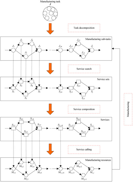
Figure 1.
CMfg SvcComp process.
3.2. SvcComp Process
Users compensate for utilizing manufacturing resources mapped by cloud services to fulfill manufacturing tasks. The procedure encompassing service discovery and composition is depicted in Figure 1. Potential cloud services suitable for a given manufacturing task can be sourced from the cloud resource pool. The set of cloud services, encompassing all atomic services capable of executing the j-th sub-task within the cloud resource pool, is mathematically represented as follows:
wherein Pj signifies the count of cloud services present in the j-th cloud service set, and designates the Pj-th cloud service belonging to the j-th cloud service set.
The aggregate count of cloud services encompassed within n cloud service sets amounts to
where N represents the overall tally of cloud services.
3.3. SvcComp Evaluation Factors
3.3.1. Time-Varying Service Credibility
Service credibility (SC) is the socialized evaluation of service transactions that occur in a certain period of time for CMfg services, SvcComp, service providers, service users and cloud service platforms. Service credibility is mainly used to reflect the impact of various subjective and social factors on service quality and SvcComp performance in CMfg, such as service reputation, communication level, social relations of manufacturing entities, etc. If the service credibility changes with time, it is called time-varying service credibility. Service score, honesty value, and visit rate are used to calculate the service credibility.
(1) Service score.
The service score refers to the score given by the user after using the CMfg service. The CMfg service platform calculates the CMfg service score according to the service score values given by all users. The calculation formula of service score is as follows:
where represents the standardized service score of the i-th CMfg service, and its value range is [0, 1]; represents the service score value given by the h-th user for the i-th CMfg service, and its value range is [0, 5]; signifies the aggregate count of users evaluating the i-th CMfg service.
(2) Service honesty.
After using CMfg services, the user can mark a CMfg service as dishonest in the dishonest record box, or recommend the service in the recommendation record box. The CMfg service platform calculates the service honesty value according to dishonest records and recommendation records as follows:
where denotes the honesty value of the i-th CMfg service; denotes the number of recommendation records for the i-th CMfg service; denotes the number of dishonest records for the i-th CMfg service.
(3) Visit rate.
CMfg services with high credibility are easy to gain the familiarity of cloud service users, which can encourage users to pay again to use them and recommend them to others, and generate greater service visits. Therefore, the visit rate serves as a metric to assess the credibility of CMfg services, and its computation formula is outlined below:
where denotes the visit rate of the i-th CMfg service; denotes the number of visits to the i-th CMfg service; and denotes the maximum visit number of the same type of CMfg service as the i-th one.
In summary, service credibility can be calculated as follows:
where SCij indicates the service credibility of the i-th CMfg service for the j-th task; β1, β2 and β3 represent the weight coefficients associated with their respective influencing factors, and β1 + β2 + β3 = 1.
The service credibility is enhanced with the increase in service transaction behavior. When transaction occurs at a certain time, the new service credibility value can be calculated according to Equation (7). If there is no transaction within a certain period of time, the service credibility declines with the passage of time, and is therefore called time-varying credibility. Its attenuation rate is proportional to the current value of service credibility. The computation formula is outlined as follows:
where is the attenuation coefficient of service credibility, and . By solving the differential equation, we can obtain that
where is the service credibility value at time t; is the initial value of at .
Combining Equations (7) and (9) can obtain that
where is a switching variable. If a CMfg service has transaction behavior at t, , and the calculated value is assigned to . If a CMfg service has no transaction behavior at t, .
3.3.2. Composition Synergy Degree
The composition synergy degree quantifies the level of collaboration among CMfg services that are integrated to fulfill complex manufacturing tasks. During SvcComp, inadequate synergy can significantly hinder information exchange and material transportation between CMfg services, thereby prolonging product delivery times. The composition synergy between CMfg services Si and Sj, utilized for executing manufacturing tasks Ji and Jj, can be computed as follows:
where CSij denotes the level of composition synergy exhibited between the i-th and j-th CMfg services within the SvcComp. Ti signifies the duration required by CMfg service Si to independently complete manufacturing task Ji, whereas Tj represents the time taken by CMfg service Sj to independently fulfill manufacturing task Jj. , and are switching variables. If manufacturing tasks and are independent and executed in parallel, ; otherwise, . Similarly, if tasks and are independent and executed sequentially, ; otherwise, . If tasks and are interactively coupled, ; otherwise, . represents a methodology for determining the aggregate execution time of manufacturing sub-tasks Ji and Jj when executed independently and in parallel. Conversely, outlines the calculation of the total execution time for Ji and Jj when executed independently but in a sequential manner. For scenarios where Ji and Jj are interactively coupled, provides the formula for computing their combined execution time. denotes the coefficient of interactive coupling between Ji and Jj, with a range spanning from −1 to 1. The value of is influenced by factors such as prior cooperation frequency and level, as well as the smoothness of service interaction and material transportation. A higher frequency and level of prior cooperation, along with smoother service interaction and material transportation, result in a lower value of ; conversely, the factors contribute to a higher value of .
3.3.3. Time-Varying Service Reliability
Service reliability (SR) serves as a quantitative metric for assessing the congruency between CMfg services and assigned manufacturing tasks. SR captures the functional alignment between cloud services and manufacturing objectives in terms of request–response interactions. When SR exhibits temporal variations, it is termed time-varying service reliability. Key determinants of service matching include the availability of manufacturing resources, equipment condition, technological proficiency, functional alignment, process prerequisites, integrated manufacturing capabilities, the cumulative count of analogous manufacturing tasks executed by CMfg services, the activity level of CMfg services, and the proximity between manufacturing resources and the service objects mapped by CMfg services. Based on their inherent characteristics, the influencing factors can be categorized as function, state, and distance factors.
(1) Function factor.
The function factor (FF) assesses the technical proficiency of CMfg services in executing manufacturing tasks, considering factors such as the past performance of similar tasks, service execution efficiency, service activity, and device performance. FFij specifically quantifies the technical capability of the i-th cloud service in fulfilling the j-th manufacturing task, with a value range of [0, 1]. Higher values of FFij indicate excellent equipment performance, high service activity and execution rates, and a substantial history of successfully completing analogous tasks. Conversely, lower values reflect poorer performance in these areas. In the case of complete mismatch between the i-th cloud service and the j-th manufacturing task, FFij is assigned a value of 0.
(2) State factor.
The state factor SFij represents the objective status evaluation of the i-th cloud service’s ability to undertake the j-th manufacturing task, ranging from 0 to 1. When CMfg services boast a high idle rate of manufacturing resources and a strong willingness to accept manufacturing tasks, SFij assumes a higher value. Conversely, a lower SFij value reflects a less favorable state in terms of resource availability and task acceptance prospects.
(3) Distance factor.
The distance factor (DF) is employed to assess the influence of the relative proximity between manufacturing resources and users on the execution of CMfg services. DFij specifically quantifies the distance impact between the manufacturing resource allocated by the i-th CMfg service and the j-th user, with a value range of [0, 1]. A shorter distance corresponds to a higher DFij value, whereas a longer distance translates to a lower DFij value.
In summary, the service reliability can be calculated based on function factor FFij, state factor SFij and distance factor DFij as follows:
where SRij stands for the service reliability exhibited by the i-th CMfg service when undertaking the j-th manufacturing task. The weight coefficients α1, α2 and α3 represent the relative importance of the respective influencing factors, and α1 + α2 + α3 = 1.
With the passage of time, the equipment performance declines due to wear and aging, and the technical level declines when it has not performed tasks for a long time. All of them cause the service reliability to decline over time. Service transaction behavior is the most important way to improve service reliability. When transaction occurs, the new service reliability value can be calculated according to Equation (12). If there is no transaction within a certain period of time, the service reliability declines with the passage of time. Its attenuation rate is proportional to the current value of service reliability. The computation formula is outlined as follows:
where is the attenuation coefficient of service reliability, and . By solving the differential equation, we can obtain that
where represents the value of at time t, whereas signifies the initial value of at .
Combining Equations (12) and (14) can obtain that
where is a switching variable. If a CMfg service has transaction behavior at t, , and the calculated value is assigned to . If a CMfg service has no transaction behavior at t, .
3.3.4. Composition Complexity
Composition complexity serves as a metric to assess the intricacy involved in SvcComp. A lower composition complexity indicates a higher degree of service reliability and a greater likelihood of successfully executing manufacturing tasks. The composition complexity can be determined using cloud entropy, as outlined below [29].
where CC is the composition complexity. The total count of CMfg services within the SvcComp scheme is represented by N. The cloud entropy specific to the i-th CMfg service is denoted as . Qi signifies the aggregate number of states the i-th CMfg service undergoes to accomplish the designated manufacturing task. STij represents the duration of the i-th CMfg service in its j-th state, while TTi denotes the overall time required for the i-th CMfg service to complete the corresponding manufacturing task. Composition complexity corresponds to the cumulative cloud entropy of all CMfg services within the SvcComp scheme. A lower sum of cloud entropy indicates a reduced composition complexity and, consequently, a superior service reliability.
3.3.5. Execution Time
The CMfg service execution time pertains to the response latency exhibited by CMfg services in addressing manufacturing tasks. Given the intricate blend of online and offline factors inherent in CMfg services, their execution time often surpasses that of conventional web services. The duration encompasses the processing time of CMfg services, auxiliary tasks like equipment maintenance and workpiece clamping, and the time expended on material transportation throughout the service execution. The primary types of CMfg SvcComp encompass sequential, parallel, choice, and cyclic compositions. The calculation of CMfg SvcComp’s execution time can be formulated as follows:
where, ET is the overall execution time of CMfg SvcComp. For each individual service within the composition, PETi represents the processing time specific to the i-th service. Similarly, AETi signifies the auxiliary time associated with the i-th service, while LETi denotes the logistics time required. Furthermore, N indicates the comprehensive count of CMfg services encompassed within the composition. When it comes to selecting services, signifies the likelihood of choosing the i-th service within the choice composition, and . Lastly, ψ represents the total number of cycles involved.
3.3.6. Execution Cost
The cost incurred by customers for utilizing CMfg services on an as-needed basis is referred to as the CMfg service execution cost. This cost encompasses various elements, including fees levied by service providers for CMfg services, expenses associated with material transportation during service execution, and charges imposed by third-party cloud platforms for their services. The computation of the execution cost for a composition of CMfg services can be performed according to the following method:
where EC represents the overall execution cost of the CMfg SvcComp. SECi specifically denotes the cost of the i-th service within the composition, whereas LECi pertains to the logistics expenses associated with the same service. Additionally, PECi stands for the service cost imposed by the cloud platform for the i-th service within the composition.
To comprehensively capture the performance and service excellence of potential CMfg services and their compositions, an analysis has been conducted focusing on service reliability and credibility. Based on the analysis, six key quality evaluation criteria have been identified: time-varying credibility, composition synergy, time-varying reliability, composition complexity, execution time, and execution cost. These criteria form the foundation for our study on CMfg SvcComp model construction, algorithm enhancement, and case analysis.
3.4. Multi-Objective Optimization Model of CMfg SvcComp
Among the above six evaluation factors, time-varying service reliability, time-varying service credibility, and composition synergy degree are positive evaluation factors, and their maximum values are expected in the optimization goal. Composition complexity, execution time, and execution cost are negative evaluation factors, and their minimum values are expected in the optimization goal. Based on the above six evaluation factors, a mathematical model for the multi-objective optimization of CMfg SvcComp is hereby established.
where , , , , and serve as the objective functions for optimizing CMfg SvcComp. Equations (19)–(21) aim to maximize overall service reliability, credibility, and composition synergy, respectively. Conversely, Equations (22)–(24) strive to minimize composition complexity, execution time, and execution cost, respectively. Equations (25)–(27) outline the constraints of CMfg SvcComp. Specifically, Equation (25) ensures that the maximum execution time for manufacturing tasks does not exceed the threshold ETthreshold. Equation (26) imposes a cost limit, ensuring that the total execution cost of manufacturing tasks remains below the threshold, ECthreshold. Finally, Equation (27) ensures that each manufacturing task is assigned to at least one CMfg service for execution. The variable serves as a switch; it takes a value of 1 if the j-th manufacturing task is assigned to the i-th CMfg service, and 0 otherwise.
4. Improved Chaos Sparrow Search Algorithm
The sparrow search algorithm, a novel swarm intelligence optimization method introduced in 2020, simulates the foraging behavior of sparrows. Although it has superior performance, it has made slow progress in addressing the challenges of multi service composition optimization and is prone to local optimization traps. To enhance its performance, the Bernoulli chaotic mapping formula is integrated, and the position calculation formulas for explorer and scouter sparrows are fine-tuned. The improvement boosts the algorithm’s search and development capabilities, leading to superior global optimization results, faster convergence, and shorter runtimes. As a result, a novel and improved approach is provided for tackling multi service composition optimization problems.
4.1. Basic Sparrow Search Algorithm
In the basic sparrow search algorithm (BSSA), a sparrow’s position corresponds to a solution. Different sparrow positions represent different solutions. There are three types of sparrows in the sparrow group, the explorer sparrow, follower sparrow, and scouter sparrow, which correspond to the three behaviors of sparrows when foraging: (1) as an explorer, searching and finding food; (2) as a follower, following the explorer for foraging; and (3) as a scouter, detecting and monitoring predator threats, providing early warning for the sparrow group, and deciding whether to give up the current food.
In the BSSA, the explorer sparrow position formula is given below.
where represents the updated position of the j-th dimension of the i-th explorer sparrow after the t-th iteration. The algorithm has a predefined maximum iteration count denoted by MaxIteNum. The variable is a randomly generated number within the range of (0, 1], ensuring a uniform distribution. , on the other hand, is a random number drawn from the standard Gaussian distribution within the interval [0, 1]. The matrix , which consists of all elements equal to 1, is related to . Additionally, signifies the total number of dimensions in . Lastly, is a randomly chosen number from the range [0, 1], and called the warning value; is a random number between [0.5, 1], and is called the safety threshold.
The follower sparrow position formula is shown as follows:
where denotes the globally optimal foraging position attained by the explorer following the (t + 1)-th iteration. Conversely, represents the globally poorest foraging position recorded after the t-th iteration. Furthermore, comprises a matrix derived from , with its elements randomly assigned to either 1 or −1, and . Lastly, NumSpa signifies the aggregate count of sparrows involved.
The scouter sparrow position formula is given below.
where represents the globally optimal foraging position achieved after the t-th iteration. serves as a step control parameter, a random number drawn from the standard Gaussian distribution within the range [0, 1]. Additionally, is a uniformly distributed random number between [−1, 1]. , and correspond to the fitness of the i-th sparrow, the global best fitness, and the global worst fitness, respectively. Lastly, is a minute value that ensures that the denominator of the formula remains nonzero, preventing any division by zero errors.
4.2. Improved Chaos Sparrow Search Algorithm
4.2.1. SvcComp Coding Method
The improved chaos sparrow search algorithm (ICSSA) employs an integer encoding approach to establish a correspondence between the position of sparrows and the SvcComp scheme. In the CMfg environment, customer manufacturing task types include the single-function requirement type and multiple-function requirement type. The single-function requirement manufacturing task can be completed directly by the atomic CMfg service mapping a single manufacturing resource. The complex manufacturing task with multiple functional requirements needs to combine more than two atomic CMfg services. The execution procedure encompasses several key steps: the decomposition of CMfg tasks, matching of cloud services, selection of services, and composition of services. A complex manufacturing task, encompassing multiple functional prerequisites, can be dismantled into m distinct sub-tasks. Each sub-task is then assigned to a suitable candidate cloud service for execution. Consequently, the SvcComp comprises m atomic cloud services, collectively fulfilling the complex manufacturing task. In the ICSSA, a cloud SvcComp can be represented by a sparrow, and the sparrow dimension is m, corresponding to m atomic cloud services. The j-th dimension of a sparrow corresponds to the set Sj of candidate cloud services for the j-th sub-task Jj within a complex manufacturing task. The set Sj encompasses all potential cloud services suitable for executing the task Jj. The numerical value of the j-th dimension signifies the specific cloud service chosen to fulfill the j-th task. Within a sparrow group encompassing NumSpa sparrows, the spatial location of the i-th sparrow can be represented by an m-dimensional vector, as detailed below.
The sparrow group can be represented by a set as outlined below.
where represents the j-th dimension of the positional vector associated with the i-th sparrow. The numerical value of signifies the specific cloud service chosen from the candidate set Sj for task Jj during the process of SvcComp. NumSpa denotes the overall count of sparrows within the sparrow group. Additionally, Figure 2 illustrates the correlation between the sparrow and the SvcComp. Furthermore, m corresponds to the dimensionality of the sparrow variable . The sparrow code values in Figure 2 represent calling the corresponding green service options and using the corresponding green manufacturing resource options.
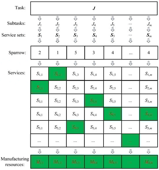
Figure 2.
The corresponding relationship between sparrow and SvcComp.
4.2.2. Fitness Function Construction
Sparrows with better fitness can obtain food first. Serving as food explorers, the sparrows steer the entire flock towards the food source. The ICSSA incorporates a weighted summation technique to formulate its fitness function. The efficacy of the ICSSA is gauged by the weighted aggregate of relative deviations across all objective functions, collectively referred to as the weighted relative deviation.
where denotes the weighted relative deviation, whereas , , , , and represent the six objective function values pertaining to the CMfg SvcComp scheme for the i-th sparrow. Additionally, , , , , and serve as the reference values for the six objective functions, established during the initialization phase of the algorithm. The reference values correspond to the objective function values of the CMfg SvcComp scheme associated with a randomly chosen sparrow. Furthermore, , , , , and represent the respective weight coefficients assigned to each of the six objective functions, and .
A smaller weighted relative deviation indicates a superior SvcComp scheme. Utilizing the formula for the weighted relative deviation, the fitness function of the ICSSA is constructed in the following manner:
where represents the fitness score of the i-th sparrow, while denotes a significantly large positive constant. The sparrow with better fitness value means that it is closer to high-quality food sources and has higher priority in obtaining food.
4.2.3. Improve the Position Formula of the Explorer Sparrow
Sparrows exhibiting superior fitness values are privileged in accessing food resources, and as such, they guide the entire sparrow population towards the food source. As evident in Equation (28), the explorer sparrow in the BSSA initially converges towards the first global optimal solution, limiting its search scope and predisposing it to local extrema, thereby compromising search precision. To address the issue, the ICSSA incorporates Bernoulli chaotic operations and the global optimal solution from the preceding generation into the position calculation formula of the explorer sparrow, as delineated in Equation (35). Bernoulli chaotic operation is used to generate chaotic sequences. It has the characteristics of nonlinearity, ergodicity, randomness, and so on. Furthermore, the updated formula takes into account the positions of both the previous generation’s explorer sparrow and the previous generation’s global optimal sparrow, thereby effectively safeguarding the algorithm from converging prematurely towards local optima.
where represents the updated position of the j-th dimension of the i-th explorer sparrow after the t-th iteration. represents the globally optimal solution attained after the completion of the t-th iteration. is a random number drawn from the standard Gaussian distribution within the interval [0, 1]. The matrix , which consists of all elements equal to 1, is related to . Additionally, signifies the total number of dimensions in . is a randomly chosen number from the range [0, 1], and is called the warning value. is a number between [0.5, 1], and is called the safety threshold. If , Equation (35) signifies the absence of predators in proximity to the explorer sparrow, enabling it to conduct a thorough search. Conversely, when , Equation (35) suggests that some sparrows have detected predators, necessitating the entire group to relocate to safer regions promptly. is the value of the t-th iteration Bernoulli chaotic sequence, and is calculated as follows.
To surpass the optimization performance achieved by the random numbers employed in the standard sparrow algorithm formula, Bernoulli chaotic operations are incorporated during the initialization phase of the sparrow population, as detailed in Equation (36).
where is the control parameter. The initial value of the Bernoulli chaotic sequence is set as a uniform random number in the (0, 1) interval.
Inspired by the concept of inertia weight, a dynamic weight factor is incorporated into the position formula of the explorer sparrow, as outlined in Equation (37). Initially, the factor assumes a larger value, facilitating effective global exploration. As the iteration nears completion, it adjusts dynamically, enabling enhanced local search capabilities and accelerated convergence.
where t means the t-th iteration. MaxIteNum signifies the utmost iteration count of the algorithm.
4.2.4. Improve the Position Formula of the Follower Sparrow
The formula for determining the position of the follower sparrow has been enhanced as follows:
where is the best foraging position of the explorer sparrows after the (t + 1)-th iteration. After the t-th iteration, represents the globally poorest foraging position. is a random number adhering to the [0, 1] standard Gaussian distribution, while is a uniformly distributed random number within the range [−1, 1]. Additionally, signifies the total sparrow population. Equation (38) stipulates that when , the follower sparrow’s position is determined by multiplying a standard Gaussian distributed random number with an exponential function with the natural number e as its base. When the sparrow population converges, its value conforms to the standard Gaussian distribution random number. When , the follower sparrow assumes a random position that lies close to the present globally optimal location.
4.2.5. Improve the Position Formula of the Scouter Sparrow
The formula for determining the position of the scouter sparrow has been enhanced as follows:
where and are the sparrow motion control coefficients, which control the sparrow motion direction and step length. and are uniformly distributed random numbers within the range of [−1, 1]. Equation (39) illustrates that when the scouter sparrow occupies the current globally optimal position, it relocates to a nearby position. The dispersion level of its new position is influenced by the disparity between the global optimal and worst positions, as well as the step size control factor . Conversely, if the sparrow is not situated at the global optimal position, it steers towards the optimal location, with the distance determined by the difference between the global optimum and its current position, along with the step size control factor .
In the ICSSA, the sparrow’s roles as explorer, follower, and scouter are interchanged. However, the proportion of sparrows with three roles remains constant, and explorers typically comprise 10% to 20% of the overall population. Serving as the foraging leader of the sparrow group, the explorer sparrow possesses a vast search area and continuously updates its position in search of food sources. The follower sparrow follows the explorer to forage for higher fitness. In order to avoid the threat of predators, the ICSSA randomly selects 10~20% of the sparrows as scouters for surveillance and warning, so as to timely warn the whole sparrow group of anti-hunting behavior when the predators appear. In the proposed algorithm, the Bernoulli chaotic operator changes the symmetry of the old sparrow search algorithm, increases the uncertainty and randomness of the searcher sparrow position in the new algorithm, and affects the position update and movement strategies of the follower and scouter sparrows. The asymmetric chaotic characteristic brings better global search ability and optimization performance to the new algorithm.
4.3. Algorithm Steps
Illustrated in Figure 3, the key procedures of the ICSSA are outlined below:
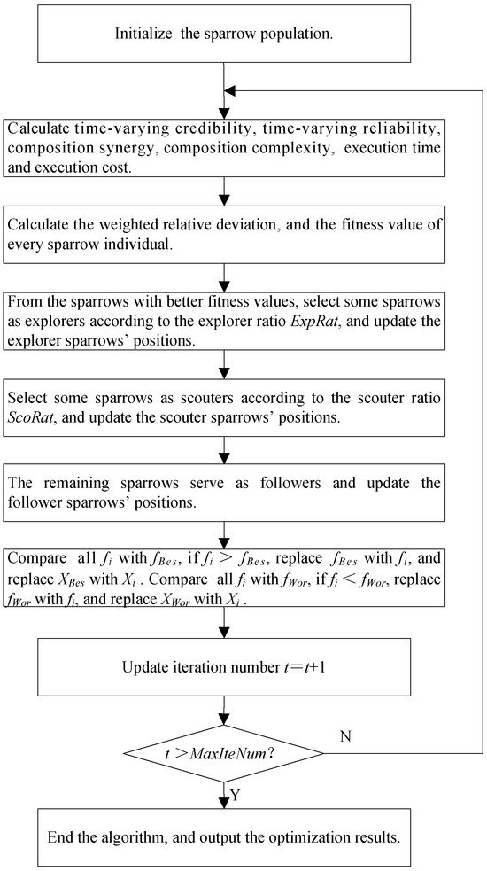
Figure 3.
ICSSA flowchart.
Step 1: Initialize the sparrow population, including the total number of sparrows, ; the maximum iteration number, ; the explorer ratio, ExpRat; the scouter ratio, ScoRat; the safety threshold, SafThr; the Bernoulli chaotic sequence control parameter, ; and so on. A sparrow is randomly selected and the six objective function values of its corresponding CMfg SvcComp scheme are taken as reference values and assigned to , , , , and .
Step 2: Calculate time-varying credibility, composition synergy, time-varying reliability, composition complexity, execution time, and execution cost.
Step 3: Determine the weighted relative deviation and fitness score for each individual sparrow.
Step 4: Select a subset of sparrows with superior fitness values as explorers, based on the explorer ratio, ExpRat, and subsequently update their positions utilizing Equation (35). Compare every explorer sparrow’s positions, and obtain the best one, .
Step 5: Select some sparrows as scouters according to the scouter ratio, ScoRat, and update the scouter sparrows’ positions utilizing Equation (39).
Step 6: The remaining sparrows assume the role of followers and undergo position updates in accordance with Equation (38).
Step 7: Compare every sparrow’s fitness value, , in the population with the global optimal fitness value, . If , replace with , and replace with . Compare with the global worst fitness value, . If , replace with , and replace with .
Step 8: Assess the termination criteria of the algorithm. If the iteration count attains the preset maximum or fulfills other designated end conditions, halt the algorithm iteration and output the result; otherwise, proceed to step 2.
5. Simulation Experiments and Analysis
5.1. Experimental Condition Setting
In order to verify the performance of the proposed ICSSA in solving multi-objective optimization problems, the WFG and DTLZ series test issues are selected, and the inverse generation distance (IGD) index and hyper volume (HV) index are used to evaluate the convergence of the algorithm and the diversity of its population. Convergence and diversity are two key metrics for multi-objective evolutionary algorithms. The algorithm achieves better diversity and convergence when the IGD value is smaller and the HV value is larger. In the experiment, each algorithm was independently run 25 times on each test question, and the results of the ICSSA were compared with the other algorithms using a rank sum test at a significance level of 0.05.
The computer configuration for the experiment is Intel Core i3-3110M CPU, 2.4 GHz main frequency, and 4G memory; the BSSA [53], PSO [3], SGA [46] and NSGA-III [54] are used as comparative algorithms. BSSA is the basic sparrow search algorithm; PSO is the particle swarm optimization algorithm; SGA is the standard genetic algorithm; and NSGA-III is the third-generation non-dominated sorting genetic algorithm. Under the same conditions, each algorithm is subjected to 25 independent experiments and compared. The population size of each algorithm is set to 120 and the number of iterations is 300. Other algorithm parameters are referenced from the corresponding literature.
5.2. Analysis of Experimental Results
Table 1 and Table 2 record the mean and variance of IGD and HV, respectively. In the tables, the preceding values represent the mean of IGD or HV, while the values in parentheses represent their standard deviation. The last row shows the test results of the ICSSA compared to other algorithms. The symbol “+” indicates that the ICSSA performs better than the other algorithms, “-” indicates that the ICSSA is inferior to the other algorithms, and “=” indicates that the ICSSA performs similarly to the other algorithms. On the mean of IGD, the ICSSA outperforms BSSA, PSO, SGA, and NSGA-III in 10 out of 15 test issues. In the other four test issues, WFG2, DTLZ2, DTLZ3, and DTLZ7, NSGA-III performs the best, and the ICSSA is second best or third best. In the WFG3 test issue, the PSO algorithm has the best test results, and the test results of the ICSSA are suboptimal. On the variance of IGD, the ICSSA has 12 out of 15 test issues with smaller variances than other algorithms. In the test issues WFG1, WFG3, WFG5, DTLZ3, and DTLZ7, the variance of the ICSSA test results is much smaller than that of BSSA PSO, SGA, and NSGA-III. On other testing issues, although the IGD variance results of the ICSSA are not the best, they all reached suboptimal levels, indicating that the ICSSA has good robustness. In terms of HV performance indicators, the ICSSA outperforms BSSA, PSO, SGA, and NSGA-III in 12 out of 15 test issues. In the test issues WFG2, DTLZ2 and DTLZ3, the NSGA-III test results are the best, and the ICSSA performs suboptimally.

Table 1.
IGD values of ICSSA, BSSA, PSO, SGA, and NSGA-III algorithm test results.
Table 2.
HV values of ICSSA, BSSA, PSO, SGA, and NSGA-III algorithm test results.
Figure 4 and Figure 5 provide box plots of the distribution of IGD and HV values, respectively, from which it can be observed that the ICSSA outperforms BSSA, PSO, SGA, and NSGA-III in most test issues, especially in the HV index, and showed good test results, indicating that the ICSSA has a wide spatial distribution range and good diversity. The ICSSA mostly outperforms other algorithms in terms of IGD metrics. In the WFG3 testing issue, the PSO algorithm achieved good results in the IGD mean test but poor results in the HV mean test, indicating that the distribution range of non-inferior solutions found by the PSO algorithm in the problem is limited. The ICSSA is suboptimal in the IGD mean test but has the best results in the HV mean and variance. Based on comprehensive analysis, regarding the WFG3 issue, the ICSSA is superior to PSO. In the testing issues of WFG2, DTLZ2 and DTLZ3, the NSGA-III algorithm has the best testing performance, but the ICSSA is suboptimal and has a small difference from the optimal value. Further in-depth research on neighborhood relationships can improve the performance of the algorithm. The above analysis indicates that the ICSSA searches for non-inferior solutions with a wide distribution and good diversity, which reduces unnecessary computational consumption while ensuring the accuracy of the solution and the convergence of the algorithm, and effectively balances the convergence and diversity in solving multi-objective problems.
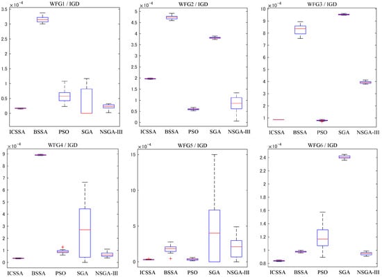
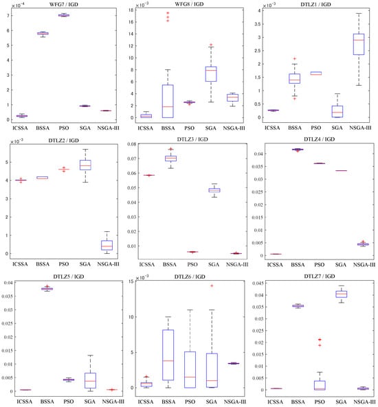
Figure 4.
Box plots of IGD distribution for ICSSA, BSSA, PSO, SGA, and NSGA-III algorithms.
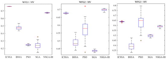
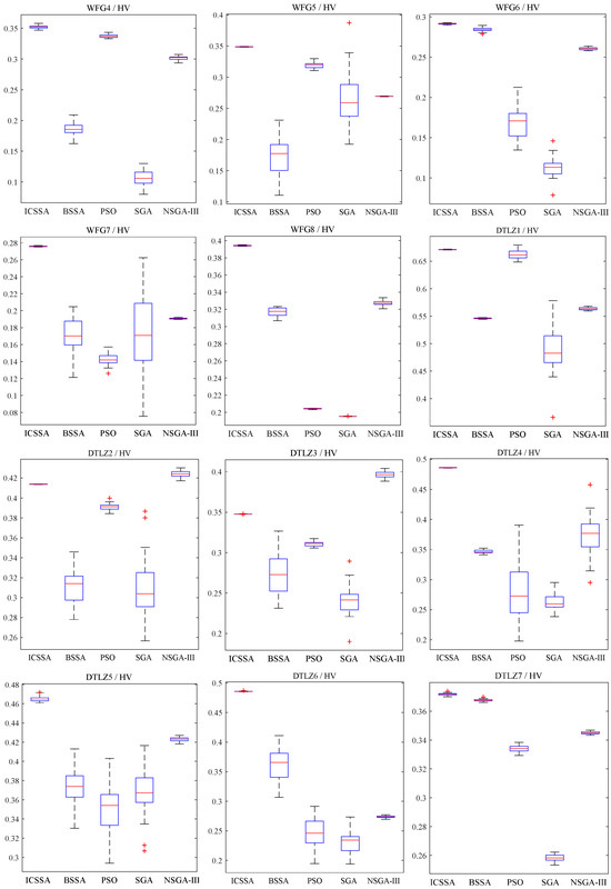
Figure 5.
Box plots of HV distribution for ICSSA, BSSA, PSO, SGA, and NSGA-III algorithms.
6. Application Example
Taking the manufacturing tasks of two disinfection robots (DRs) based on CMfg SvcComp as an example, the above SvcComp model and ICSSA are applied and analyzed.
A manufacturing task for a DR can be segmented into five distinct sub-tasks: the robot body production sub-task, J1; the driver module production sub-task, J2; the painting sub-task, J3; the disinfection module production sub-task, J4; and the electrical control module production sub-task, J5. The five sub-tasks are independent of each other. J1, J2, J4 and J5 are parallel relations, and they all have sequence relations with J3. The alignment of manufacturing tasks with cloud services, as determined by the ICSSA, is outlined in Table 3. Specifically, manufacturing tasks J1, J2, J3, J4 and J5 correspond to cloud service sets S1, S2, S3, S4 and S5, which encompass 4, 2, 3, 5, and 4 cloud services, respectively. SS, SH and VR represent the service score factor, service honesty factor, and visit rate factor. ET, LET, PET and AET represent execution time [hours], logistics time [hours], continuous processing time [hours] and auxiliary time [hours] for equipment maintenance, respectively. UC represents the unit time execution cost [USD/hour]. PEC represents cloud platform service cost [USD]. Time-varying service reliability, SR, is calculated according to Equation (15), and α1 = 0.4, α2 = 0.3 and α3 = 0.3. According to Equations (10) and (16), time-varying service credibility, SC, and composition complexity, CC, are calculated, respectively, and β1 = 0.3, β2 = 0.4 and β3 = 0.3. The calculation results are shown in Table 3. RR represents the number of recommendation records. DR represents the number of dishonest records. The users’ scoring values, US, are shown in Table 4, where represents the h-th user’s scoring value for the i-th CMfg service. The attenuation coefficient values are .
Table 3.
Matching relationship between cloud services and manufacturing tasks.
Table 4.
User’s scoring value.
According to Equation (11), the SvcComp synergy values of DR manufacturing tasks are calculated and shown in Table 5.
Table 5.
Calculation results of service composition synergy.
The program of the ICSSA is written in MATLAB R2015a. The execution time constraint ETthreshold is 500 h, and the execution cost constraint ECthreshold is USD 70,000. The sparrow population NumSpa comprises 50 individuals, and the maximum iteration count MaxIteNum is set to 180. Γ = 99 and λ = 0.5. The weight coefficients for six objective functions are designated as δ1 = δ3 = δ5 = δ6 = 0.2 and δ2 = δ4 = 0.1. After 87 iterations, the ICSSA converges and the population optimal fitness value is 99.101. In the corresponding optimal SvcComp scheme, the time-varying service reliability is 6.161, the composition complexity is 8.81, the time-varying service credibility is 7.085, the composition synergy is 40.854, the execution time is 182 h, and the execution cost is USD 33,921. The optimal SvcComp scheme is represented by the sparrow position code 4114342313. The code’s interpretation, as depicted in Figure 6, is as follows: for the first DR manufacturing task J1,1, the fourth cloud service from set S1 is selected; for J2,1, the first service from S2 is selected; for J3,1, the first from S3 is selected; for J4,1, the fourth from S4 is selected; and for J5,1, the third from S5 is selected. Similarly, for the second DR manufacturing task, J1,2 selects the fourth service from S1; for J2,2, the second from S2 is selected; for J3,2, the third from S3 is selected; for J4,2, the first from S4 is selected; and for J5,2, the third from S5 is selected. The average execution time stands at 18.73 s, and the iteration curves pertaining to its key parameters are exhibited in Figure 7. Figure 7a shows the time-varying service reliability iteration curve; Figure 7b shows the time-varying service credibility iteration curve. When the sparrow population iterates to the 87th iteration, the algorithm tends to be stable. The optimal individual fitness iteration curve is shown as the red curve in Figure 8.

Figure 6.
The optimal solution of DR manufacturing tasks.
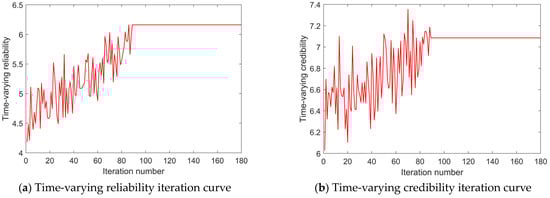
Figure 7.
ICSSA iteration curves.
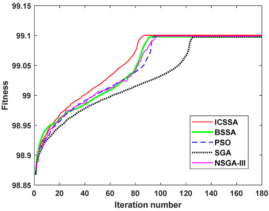
Figure 8.
Comparison of ICSSA, BSSA, PSO, SGA and NSGA-III iteration curves.
In the case of the same maximum iteration number and total number of sparrows, five algorithms such as the ICSSA, BSSA [53], PSO [3], SGA [46] and NSGA-III [54] are employed to address the identical SvcComp optimization problem. According to Figure 8, the ICSSA attains the optimal solution in the 87th iteration, BSSA in the 92nd, PSO in the 95th, SGA in the 126th, and NSGA-III in the 97th iteration. All five algorithms were tested on the same portable computer, featuring an Intel Core i3-3110M CPU, a 2.4 GHz main frequency, and 4G of memory. The equipment is manufactured by Lenovo in Shenzhen, China. It takes 18.73 s for ICSSA, 19.25 s for BSSA, 19.81 s for PSO, 26.68 s for SGA, and 20.54 s for NSGA-III. The preceding experimental outcomes clearly demonstrate that when addressing the multi-objective optimization challenge of CMfg SvcComp, the ICSSA exhibits superior convergence velocity and reduced solution time in comparison to the BSSA, PSO, SGA, and NSGA-III. As evident in Table 6, the SvcComp strategy generated by the ICSSA surpasses both the Minimum Execution Time Service Composition scheme (METSC) and the Minimum Execution Cost Service Composition scheme (MECSC) in terms of service reliability, credibility, and composition synergy. Furthermore, when compared to the outcomes of other algorithms, the ICSSA achieves the lowest weighted relative deviation and offers the finest overall quality of service. Overall, the ICSSA boasts the most comprehensive performance, which greatly aids users in making more rational decisions from the perspective of the overall service quality of cloud SvcComp. It can help enterprises build a better and more reliable manufacturing industry chain in today’s complex and volatile international environment.
Table 6.
Comparison of DR manufacturing task SvcComp optimization results.
7. Conclusions
Given the significance of manufacturing entity reliability and service reputation in shaping the transformation and progress of the manufacturing industry in the new era, this paper delves into the analysis and examination of CMfg services’ time-varying reliability and credibility. Additionally, it explores the application of the ICSSA in addressing the multi-objective optimization challenges associated with CMfg SvcComp, along with the establishment of a comprehensive evaluation model that takes into account both time-varying reliability and credibility. The key contributions of this paper can be summarized as follows.
(1) The primary factors influencing the performance of CMfg SvcComp are thoroughly investigated, including the quantitative methods of time-varying reliability and time-varying credibility of CMfg services. Combining the four new attributes of time-varying reliability, composition complexity, time-varying credibility, and composition synergy with the two traditional attributes of execution time and execution cost, integrating subjective and objective factors and natural and social factors, a new CMfg SvcComp service quality model is constructed, and the individual fitness function is constructed by the weighted sum method. The comprehensive performance of the SvcComp is assessed using the weighted relative deviation. A smaller weighted relative deviation indicates superior overall performance of the SvcComp.
(2) A refined chaos sparrow search algorithm is introduced to address the optimization model for CMfg SvcComp. The enhanced approach incorporates the Bernoulli chaotic mapping formula to enhance the sparrow search algorithm. Furthermore, modifications are made to the position calculation formulas for both the explorer and scouter sparrows. The modifications not only enhance the algorithm’s global search capabilities during its initial stages, but also mitigate premature convergence, resulting in a more comprehensive solution space. Additionally, the algorithm is designed to focus on local fine searches in its later stages, thereby improving optimization accuracy.
(3) The WFG and DTLZ test function series are chosen for analysis, and the inverse generation distance (IGD) index and the hyper volume (HV) index are utilized to assess the convergence and diversity characteristics of various algorithms including the ICSSA, BSSA, PSO, SGA, and NSGA-III. Through simulation experiments, it is evident that the ICSSA demonstrated superior performance in a majority of the testing scenarios. Specifically, with regard to the IGD mean, the ICSSA exhibited lower mean values in 12 out of 15 test issues compared to the other algorithms. Similarly, in terms of HV performance, the ICSSA surpassed BSSA, PSO, SGA, and NSGA-III in 12 of the 15 test cases.
(4) Utilizing DR manufacturing tasks as a representative example, the proposed multi-objective optimization model and algorithm for CMfg SvcComp are implemented, contrasted, and thoroughly analyzed. Their effectiveness is confirmed through rigorous verification. This case study demonstrates that, in comparison to BSSA, SGA, and PSO, the ICSSA exhibits superior solution quality and a swifter convergence rate for addressing the multi-objective optimization problem related to CMfg SvcComp. The SvcComp scheme solved by the ICSSA has better comprehensive performance, which is helpful for cloud service users to make more reasonable decisions.
Author Contributions
Conceptualization, Y.L. and X.Y.; methodology, Y.L.; software, S.W.; validation, W.X.; formal analysis, Z.Y.; investigation, W.X.; resources, Y.L.; data curation, S.W.; writing—original draft preparation, Y.L.; writing—review and editing, Y.L.; visualization, Y.L.; supervision, Z.Y.; project administration, X.Y.; funding acquisition, X.Y., Y.L. and S.W. All authors have read and agreed to the published version of the manuscript.
Funding
This research was funded by the National Natural Science Foundation of China (Grant No. 51375168), the Natural Science Foundation of Bijie City (Grant Nos. BKLHZ G[2019]8, BKLH[2023]9), the Natural Science Research Project of Guizhou Higher Education Institutions of China (Grant Nos. QJJ[2023]047, QJJ[2023]093), and the Natural Science Research Project of Education Department of Guizhou of China (Grant No. QJJ[2022]398).
Data Availability Statement
All of the data are in the article, no other new data are created.
Conflicts of Interest
The authors declare no conflicts of interest.
References
- Zhou, J.; Gao, L.; Lu, C.; Yao, X. Transfer learning assisted batch optimization of jobs arriving dynamically in manufacturing cloud. J. Manuf. Syst. 2022, 65, 44–58. [Google Scholar] [CrossRef]
- Yin, C.; Li, S.; Li, X. An optimization method of cloud manufacturing service composition based on matching-collaboration degree. Int. J. Adv. Manuf. Technol. 2024, 131, 343–353. [Google Scholar] [CrossRef]
- Ali, M.T.N.; Mirsaeid, S.H.; Homayun, M. Reliability-aware web service composition with cost minimization perspective: A multi-objective particle swarm optimization model in multi-cloud scenarios. Soft Comput. 2023, 28, 5173–5196. [Google Scholar]
- Delaram, J.; Houshamand, M.; Ashtiani, F.; Fatahi Valilai, O. Development of public cloud manufacturing markets: A mechanism design approach. Int. J. Syst. Sci. Oper. Logist. 2023, 10, 2079751. [Google Scholar] [CrossRef]
- Jin, H.; Jiang, C.; Lv, S. A hybrid whale optimization algorithm for quality of service-aware manufacturing cloud service composition. Symmetry 2023, 16, 46. [Google Scholar] [CrossRef]
- Zhao, Q.-Y.; Wei, L.; Shu, H.-P. Research on credibility support mechanism of manufacturing cloud service based on classified QoS. In Proceedings of the 5th International Asia Conference on Industrial Engineering and Management Innovation (IEMI2014); Atlantis Press: Paris, France, 2015; Volume 1, pp. 67–70. [Google Scholar]
- Aamir, T.; Dong, H.; Bouguettaya, A. Stance and credibility based trust in social-sensor cloud services. Web Inf. Syst. Eng. 2018, 11234, 178–189. [Google Scholar]
- Tang, R.; Yue, Y.; Ding, X.; Qiu, Y. Credibility-based cloud media resource allocation algorithm. J. Netw. Comput. Appl. 2014, 46, 315–321. [Google Scholar] [CrossRef]
- Wang, S.; Lu, W.; Du, Z. A approach of credibility-based trust management service in cloud environments. Adv. Mechatron. Control Eng. 2013, 278–280, 1771–1778. [Google Scholar] [CrossRef]
- Qu, L.; Wang, Y.; Orgun, M.; Wong, D.S.; Bouguettaya, A. Evaluating cloud users’ credibility of providing subjective assessment or objective assessment for cloud services. Serv.-Oriented Comput. 2014, 8831, 453–461. [Google Scholar]
- Cai, X.; Zhang, M.; Hu, J.; Wu, Q. A reputation revision method based on the credibility for cloud services. In Proceedings of the 3rd Internatioinal Conference on Mechatronics and Industrial Informatics, Zhuhai, China, 30–31 October 2015; Volume 31, pp. 581–586. [Google Scholar]
- Mubarok, K.; Xu, X.; Ye, X.; Zhong, R.Y.; Lu, Y. Manufacturing service reliability assessment in cloud manufacturing. Procedia CIRP 2018, 72, 940–946. [Google Scholar] [CrossRef]
- Liu, J.; Chen, Y. A personalized clustering-based and reliable trust-aware QoS prediction approach for cloud service recommendation in cloud manufacturing. Knowl.-Based Syst. 2019, 174, 43–56. [Google Scholar] [CrossRef]
- Jing, S.K.; Jiang, H.; Xu, W.T.; Zhou, J.T. Cloud manufacturing service composition considering execution reliability. J. Comput.-Aided Des. Comput. Graph. 2014, 26, 392–400. [Google Scholar]
- Jiang, C.; Qiu, H.; Gao, L.; Wang, D.; Yang, Z.; Chen, L. Real-time estimation error-guided active learning Kriging method for time-dependent reliability analysis. Appl. Math. Model. 2019, 77, 82–98. [Google Scholar] [CrossRef]
- Junejo, A.K.; Jokhio, I.A.; Jan, T. A multi-dimensional and multi-factor trust computation framework for cloud services. Electronics 2022, 11, 1932. [Google Scholar] [CrossRef]
- Wan, Z.; Chen, J.; Li, J.; Ang, A.H.-S. An efficient new PDEM-COM based approach for time-variant reliability assessment of structures with monotonically deteriorating materials. Struct. Saf. 2019, 82, 101878. [Google Scholar] [CrossRef]
- Qian, H.-M.; Huang, H.-Z.; Li, Y.-F. A novel single-loop procedure for time-variant reliability analysis based on Kriging model. Appl. Math. Model. 2019, 75, 735–748. [Google Scholar] [CrossRef]
- Li, H.-S.; Wang, T.; Yuan, J.-Y.; Zhang, H. A sampling-based method for high-dimensional time-variant reliability analysis. Mech. Syst. Signal Process. 2019, 126, 505–520. [Google Scholar] [CrossRef]
- Ping, M.; Han, X.; Jiang, C.; Xiao, X. A time-variant extreme-value event evolution method for time-variant reliability analysis. Mech. Syst. Signal Process. 2019, 130, 333–348. [Google Scholar] [CrossRef]
- Liu, M.; Wang, Q.; Ling, L. Cloud manufacturing task decomposition method based on HTN. China Mech. Eng. 2017, 28, 924–929. [Google Scholar]
- Liu, A.; Pfund, M.; Fowler, J. Scheduling optimization of task allocation in integrated manufacturing system based on task decomposition. J. Syst. Eng. Electron. 2016, 27, 422–433. [Google Scholar] [CrossRef]
- Yi, S.; Tan, M.; Guo, Z.; Wen, P.; Zhou, J. Manufacturing task decomposition optimization in cloud manufacturing service platform. Comput. Integr. Manuf. Syst. 2015, 21, 2201–2212. [Google Scholar]
- Dmitriy, K.; Baruch, S.; Hadas, S. Flexible resource allocation to interval jobs. Algorithmica 2019, 81, 3217–3244. [Google Scholar]
- Thekinen, J.; Panchal, J.H. Resource allocation in cloud-based design and manufacturing: A mechanism design approach. J. Manuf. Syst. 2017, 43, 327–338. [Google Scholar] [CrossRef]
- Morariu, O.; Borangiu, T.; Morariu, C.; Răileanu, S. Service oriented mechanisms for smart resource allocation in private manufacturing clouds. Explor. Serv. Sci. 2016, 247, 367–383. [Google Scholar]
- Lin, Y.-K.; Chong, C.S. Fast GA-based project scheduling for computing resources allocation in a cloud manufacturing system. J. Intell. Manuf. 2017, 28, 1189–1201. [Google Scholar] [CrossRef]
- Sheng, B.; Zhang, C.; Yin, X.; Lu, Q.; Cheng, Y.; Xiao, T.; Liu, H. Common intelligent semantic matching engines of cloud manufacturing service based on OWL-S. Int. J. Adv. Manuf. Technol. 2016, 84, 103–118. [Google Scholar] [CrossRef]
- Tao, F.; Cheng, J.; Cheng, Y.; Gu, S.; Zheng, T.; Yang, H. SDMSim: A manufacturing service supply–demand matching simulator under cloud environment. Robot. Comput.-Integr. Manuf. 2017, 45, 34–46. [Google Scholar] [CrossRef]
- Zhao, J.; Wang, X. Two-sided matching model of cloud service based on QoS in cloud manufacturing environment. Comput. Integr. Manuf. Syst. 2016, 22, 104–112. [Google Scholar]
- Lu, Y.; Xu, X. A semantic web-based framework for service composition in a cloud manufacturing environment. J. Manuf. Syst. 2017, 42, 69–81. [Google Scholar] [CrossRef]
- Lartigau, J.; Xu, X.; Nie, L.; Zhan, D. Cloud manufacturing service composition based on QoS with geo-perspective transportation using an improved artificial bee colony optimization algorithm. Int. J. Prod. Res. 2015, 53, 4380–4404. [Google Scholar] [CrossRef]
- Pisching, M.A.; Junqueira, F.; Filho, D.J.S.; Miyagi, P.E. Service composition in the cloud-based manufacturing focused on the industry 4.0. In Technological Innovation for Cloud-Based Engineering Systems; Springer International Publishing: Cham, Switzerland, 2015; Volume 450, pp. 65–72. [Google Scholar]
- Xiao, Y.; Li, C.; Song, L.; Yang, J.; Su, J. A multidimensional information fusion-based matching decision method for manufacturing service resource. IEEE Access 2021, 2021, 39839–39851. [Google Scholar] [CrossRef]
- Bouzary, H.; Frank Chen, F. A hybrid grey wolf optimizer algorithm with evolutionary operators for optimal QoS-aware service composition and optimal selection in cloud manufacturing. Int. J. Adv. Manuf. Technol. 2019, 101, 2771–2784. [Google Scholar] [CrossRef]
- Fazeli, M.M.; Farjami, Y.; Nickray, M. An ensemble optimisation approach to service composition in cloud manufacturing. Int. J. Comput. Integr. Manuf. 2019, 32, 83–91. [Google Scholar] [CrossRef]
- He, K.; Zhu, D. Quality evaluation of cloud manufacturing service. Comput. Integr. Manuf. Syst. 2018, 24, 53–62. [Google Scholar]
- Wang, S.; Liu, Z.; Sun, Q.; Zou, H.; Yang, F. Towards an accurate evaluation of quality of cloud service in service-oriented cloud computing. J. Intell. Manuf. 2014, 25, 283–291. [Google Scholar] [CrossRef]
- Wang, X.; Sheng, B.; Zhang, C.; Xiao, Z.; Wang, H.; Zhao, F. An effective application of 3D cloud printing service quality evaluation in BM-MOPSO. Concurr. Comput. Pract. Exp. 2018, 30, e4977. [Google Scholar] [CrossRef]
- Ye, Y. Study the evaluation system about E-government quality of service based on the customer perception. In Proceedings of the 2016 6th International Conference on Information Technology for Manufacturing Systems; DEStech Publications Inc.: Lancaster, PA, USA, 2016; pp. 323–327. [Google Scholar]
- Hu, Y.; Pan, L.; Lv, W.; Wang, Z. Optimal selection of cloud manufacturing resources based on bacteria foraging optimization. Int. J. Comput. Integr. Manuf. 2024, 37, 165–182. [Google Scholar] [CrossRef]
- Li, Y.; Yao, X.; Zhou, J. Multi-objective optimization of cloud manufacturing service composition with cloud-entropy enhanced genetic algorithm. Stroj. Vestn.-J. Mech. Eng. 2016, 62, 577–590. [Google Scholar] [CrossRef]
- Xu, W.; Tian, S.; Liu, Q.; Xie, Y.; Zhou, Z.; Pham, D.T. An improved discrete bees algorithm for correlation-aware service aggregation optimization in cloud manufacturing. Int. J. Adv. Manuf. Technol. 2016, 84, 17–28. [Google Scholar] [CrossRef]
- Onaizah, N.A.; Aljanabi, R.M. Modelling of African vulture optimization algorithm with deep learning-based object classification for intelligent manufacturing systems. J. Smart Internet Things 2023, 2023, 62–83. [Google Scholar] [CrossRef]
- Tavana, M.; Shahdi-Pashaki, S.; Teymourian, E.; Santos-Arteaga, F.J.; Komaki, M. A discrete cuckoo optimization algorithm for consolidation in cloud computing. Comput. Ind. Eng. 2018, 115, 495–511. [Google Scholar] [CrossRef]
- Seghir, F.; Khababa, A. A hybrid approach using genetic and fruit fly optimization algorithms for QoS-aware cloud service composition. J. Intell. Manuf. 2018, 29, 1773–1792. [Google Scholar] [CrossRef]
- Wei, X.; Liu, H. A cloud manufacturing resource allocation model based on ant colony optimization algorithm. Int. J. Grid Distrib. Comput. 2015, 8, 55–66. [Google Scholar] [CrossRef]
- Que, Y.; Zhong, W.; Chen, H.; Chen, X.; Ji, X. Improved adaptive immune genetic algorithm for optimal QoS-aware service composition selection in cloud manufacturing. Int. J. Adv. Manuf. Technol. 2018, 96, 4455–4465. [Google Scholar] [CrossRef]
- Jiang, H.; Yi, J.; Chen, S.; Zhu, X. A multi-objective algorithm for task scheduling and resource allocation in cloud-based disassembly. J. Manuf. Syst. 2016, 41, 239–255. [Google Scholar] [CrossRef]
- Vila, S.; Guirado, F.; Lerida, J.L.; Cores, F. Energy-saving scheduling on IaaS HPC cloud environments based on a multi-objective genetic algorithm. J. Supercomput. 2019, 75, 1483–1495. [Google Scholar] [CrossRef]
- Li, T.; Yin, Y.; Yang, B.; Hou, J.; Zhou, K. A self-learning bee colony and genetic algorithm hybrid for cloud manufacturing services. Computing 2022, 104, 1977–2003. [Google Scholar] [CrossRef]
- Wang, Z.; Wang, S.; Yang, B.; Wang, Y.; Chen, R. A novel hybrid algorithm for large-scale composition optimization problems in cloud manufacturing. Int. J. Comput. Integr. Manuf. 2021, 34, 898–919. [Google Scholar] [CrossRef]
- Gad, A.G.; Sallam, K.M.; Chakrabortty, R.K.; Ryan, M.J.; Abohany, A.A. An improved binary sparrow search algorithm for feature selection in data classification. Neural Comput. Appl. 2022, 34, 15705–15752. [Google Scholar] [CrossRef]
- Ruiz-Vélez, A.; García, J.; Alcalá, J.; Yepes, V. Enhancing robustness in precast modular frame optimization: Integrating NSGA-II, NSGA-III, and RVEA for sustainable infrastructure. Mathematics 2024, 12, 1478. [Google Scholar] [CrossRef]
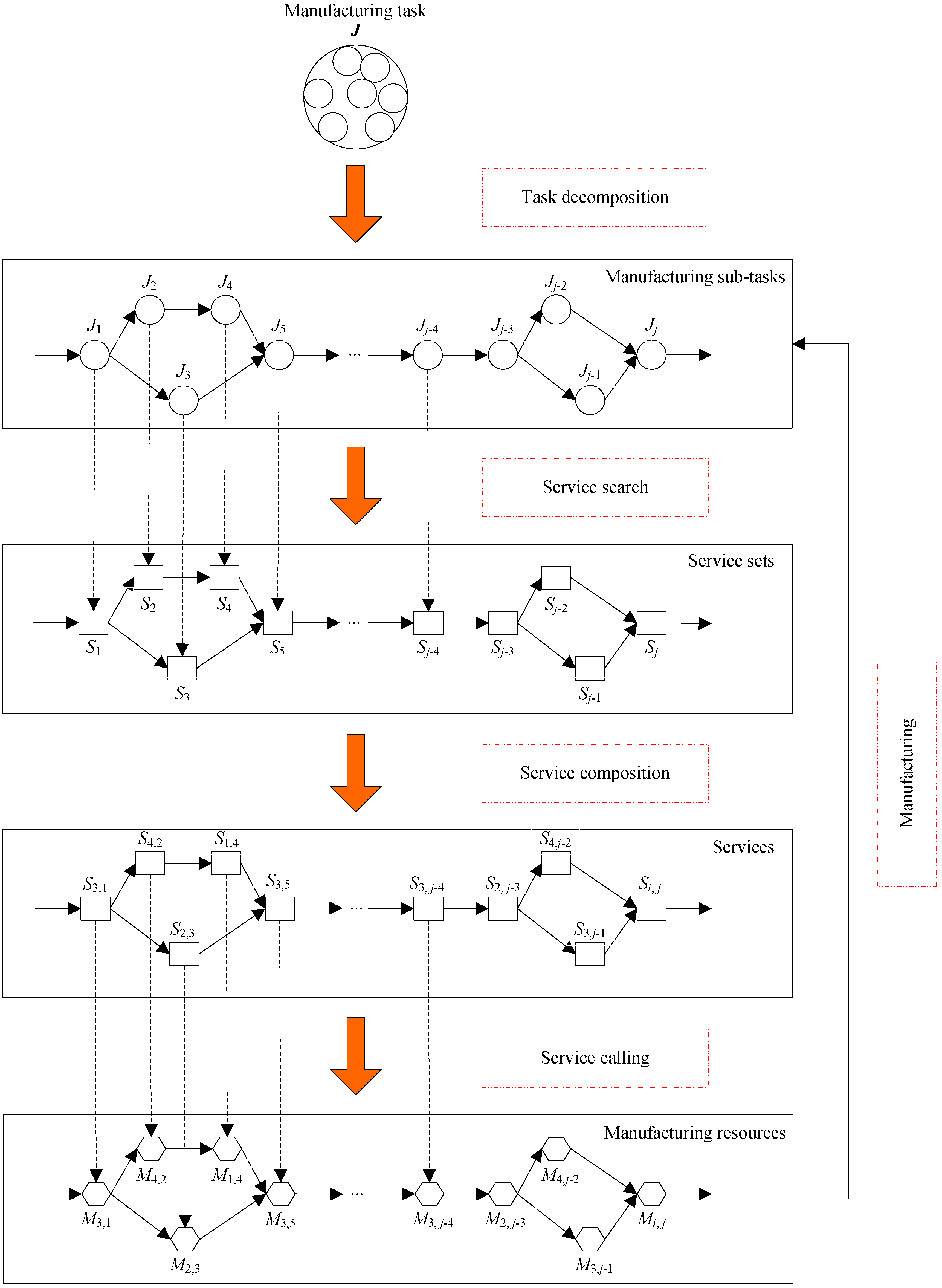

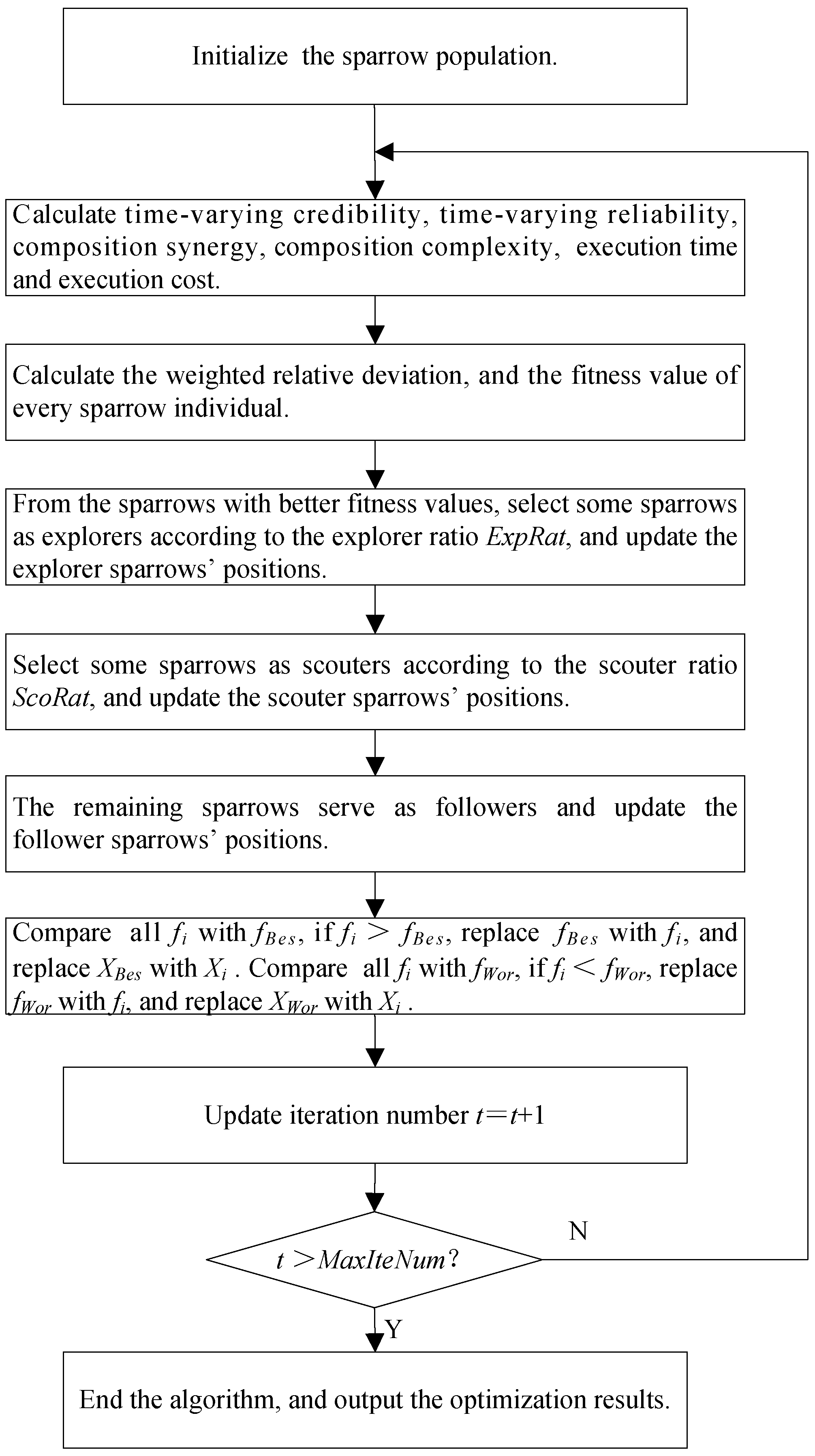
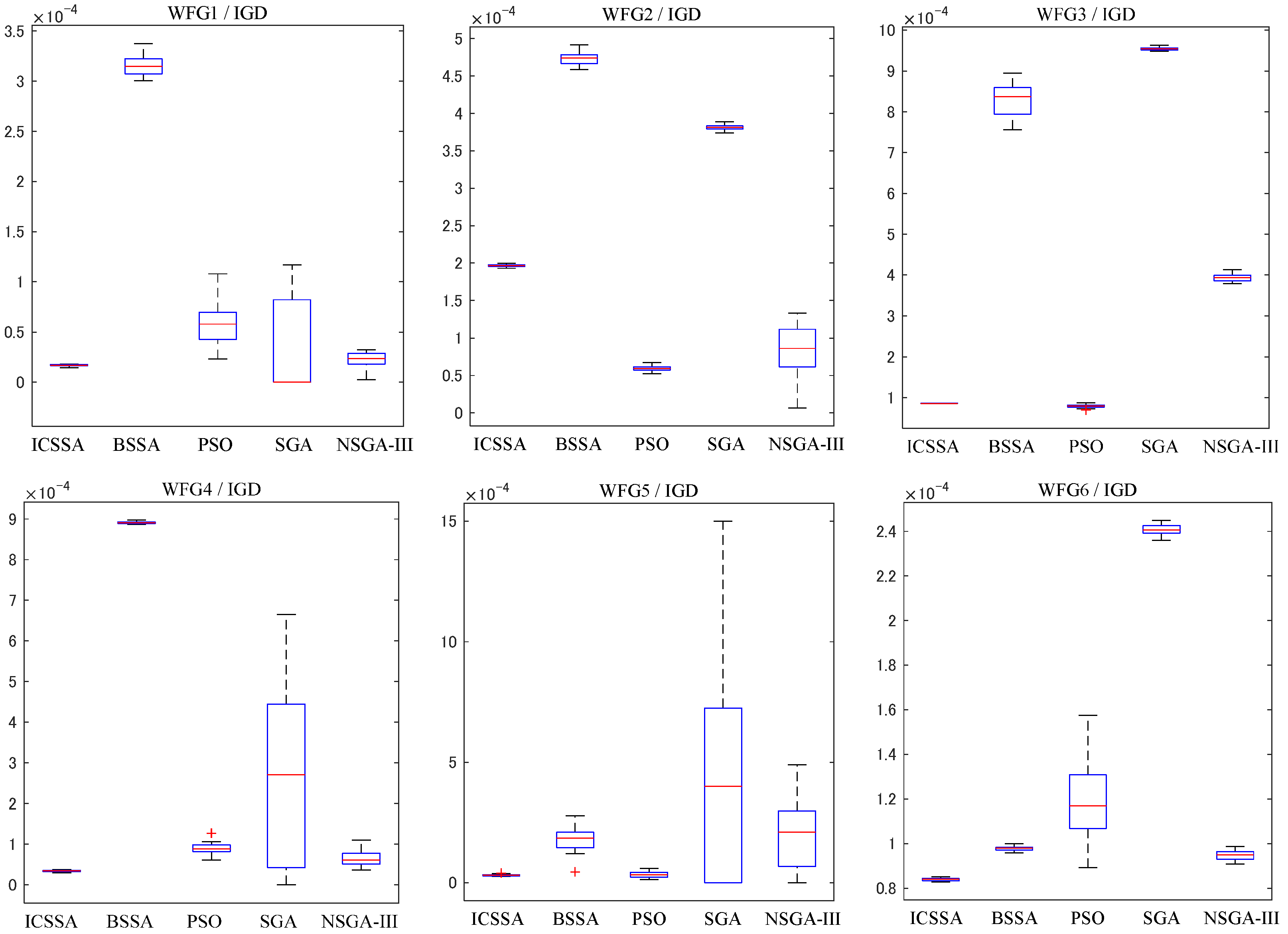
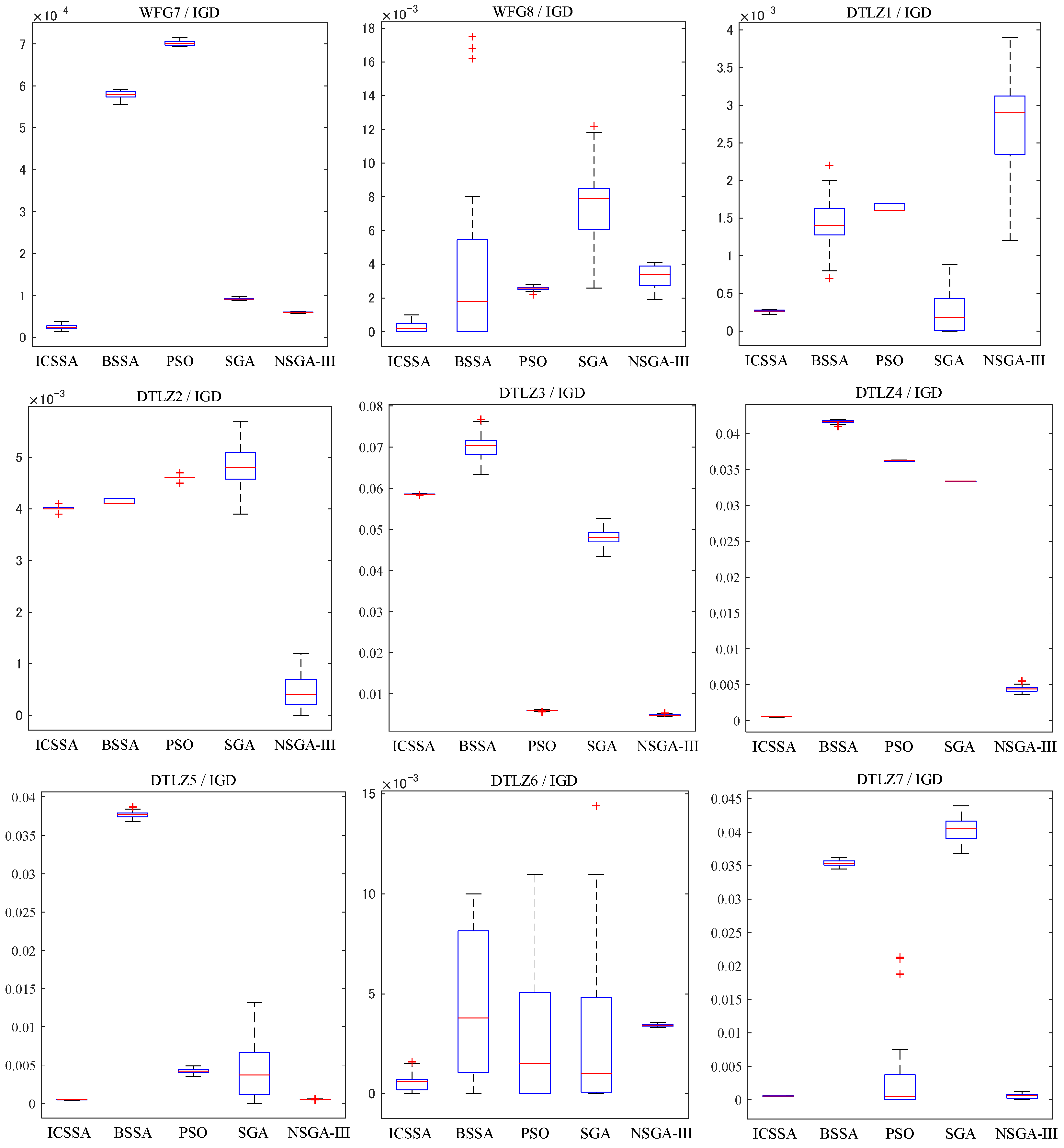
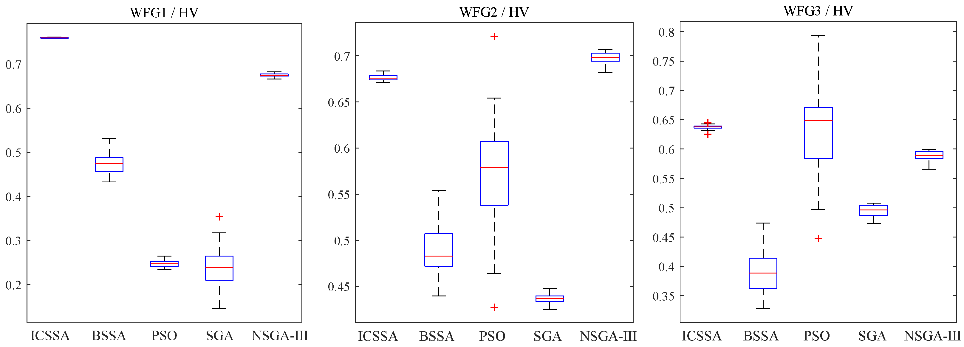
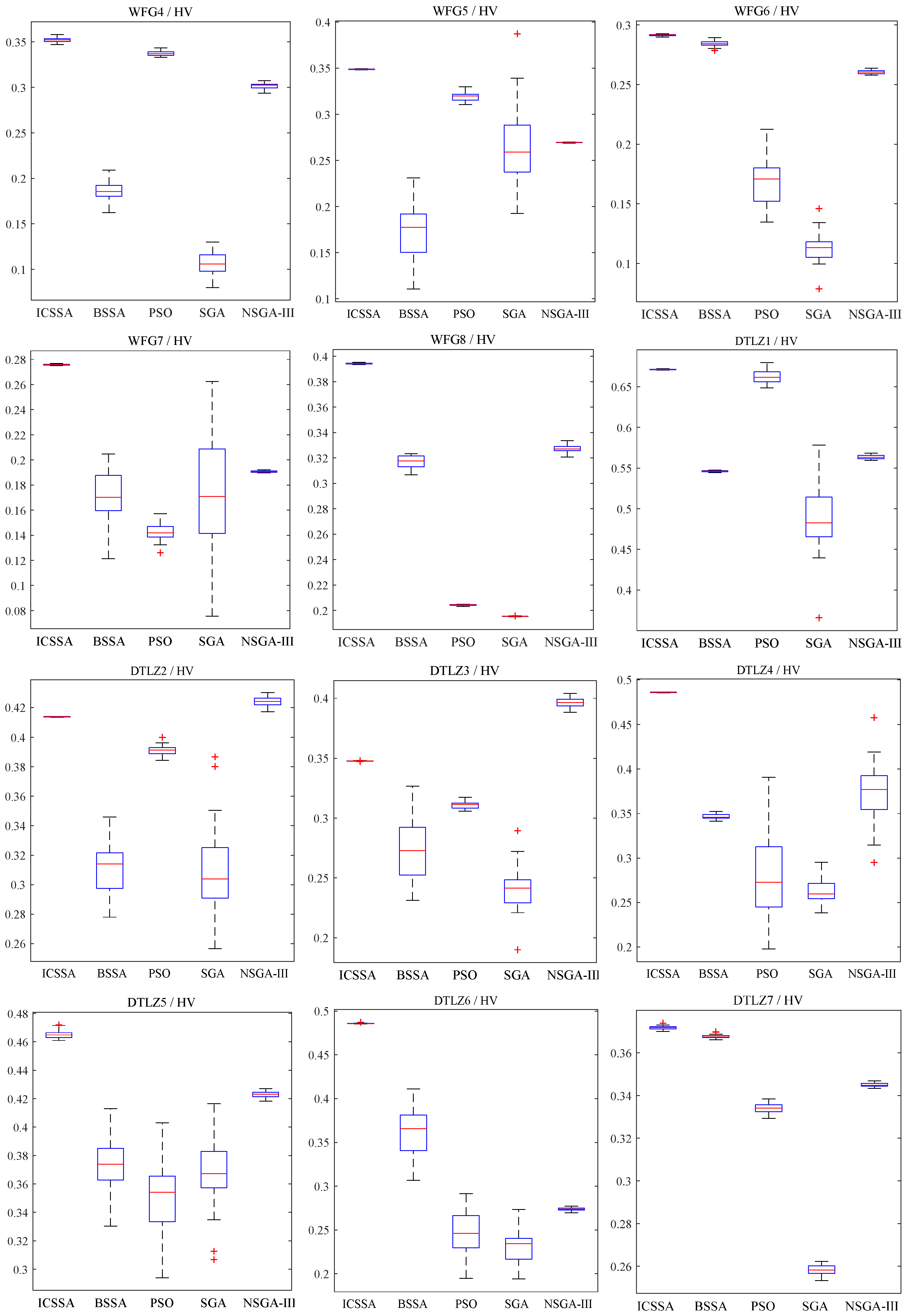
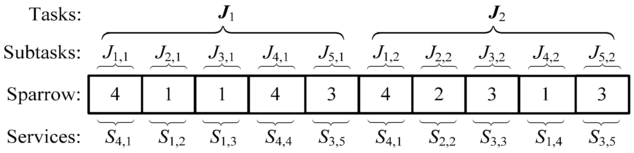
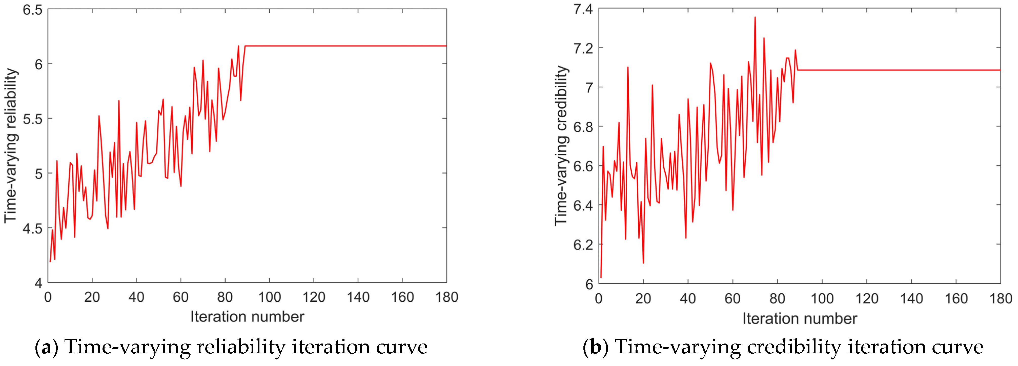

Disclaimer/Publisher’s Note: The statements, opinions and data contained in all publications are solely those of the individual author(s) and contributor(s) and not of MDPI and/or the editor(s). MDPI and/or the editor(s) disclaim responsibility for any injury to people or property resulting from any ideas, methods, instructions or products referred to in the content. |
© 2024 by the authors. Licensee MDPI, Basel, Switzerland. This article is an open access article distributed under the terms and conditions of the Creative Commons Attribution (CC BY) license (https://creativecommons.org/licenses/by/4.0/).