Stability and Numerical Simulation of a Nonlinear Hadamard Fractional Coupling Laplacian System with Symmetric Periodic Boundary Conditions

Abstract

The Hadamard fractional derivative and integral are important parts of fractional calculus which have been widely used in engineering, biology, neural networks, control theory, and so on. In addition, the periodic boundary conditions are an important class of symmetric two-point boundary conditions for differential equations and have wide applications. Therefore, this article considers a class of nonlinear Hadamard fractional coupling $(p_1,p_2)$-Laplacian systems with periodic boundary value conditions. Based on nonlinear analysis methods and the contraction mapping principle, we obtain some new and easily verifiable sufficient criteria for the existence and uniqueness of solutions to this system. Moreover, we further discuss the generalized Ulam–Hyers (GUH) stability of this problem by using some inequality techniques. Finally, three examples and simulations explain the correctness and availability of our main results.

1. Introduction

In this article, we consider the following nonlinear Hadamard fractional coupling $(p_1,p_2)$-Laplacian system with periodic boundary value conditions

$$\begin{array}{c}\hfill \left\{\begin{array}{c}{ }^H{\mathcal{D}}_{1^{+}}^{{\alpha }_1}\left[{\Phi }_{p_1}\left({ }^H{\mathcal{D}}_{1^{+}}^{{\beta }_1}{u}_1\left(t\right)\right)\right]=f_1(t,u_1\left(t\right),u_2\left(t\right)),t\in (1,e],\hfill \\ { }^H{\mathcal{D}}_{1^{+}}^{{\alpha }_2}\left[{\Phi }_{p_2}\left({ }^H{\mathcal{D}}_{1^{+}}^{{\beta }_2}{u}_2\left(t\right)\right)\right]=f_2(t,u_1\left(t\right),u_2\left(t\right)),t\in (1,e],\hfill \\ u_1\left(1\right)=u_1\left(e\right),{ }^H{\mathcal{D}}_{1^{+}}^{{\beta }_1}{u}_1\left(1\right)={ }^H{\mathcal{D}}_{1^{+}}^{{\beta }_1}{u}_1\left(e\right),\hfill \\ u_2\left(1\right)=u_2\left(e\right),{ }^H{\mathcal{D}}_{1^{+}}^{{\beta }_2}{u}_2\left(1\right)={ }^H{\mathcal{D}}_{1^{+}}^{{\beta }_2}{u}_2\left(e\right).\hfill \end{array}\right.\end{array}$$

(1)

where $1<{\alpha }_i\le 2$, $1<{\beta }_i\le 2$, $p_i>1,{ }^H{\mathcal{D}}_{1^{+}}^{*}$ represents the Hadamard fractional derivative of $*$-order and ${\Phi }_{p_i}\left(x\right)={\left|x\right|}^{p_i-2}x$ are $p_i$-Lapacian operators with inverses ${\Phi }_{p_i}^{-1}={\Phi }_{q_i}$, provided that $\frac{1}{p_i}+\frac{1}{q_i}=1$, $f_i\in C([1,e]\times {\mathbb{R}}^2,\mathbb{R})$, $i=1,2$.

Hadamard [1] first proposed Hadamard fractional calculus in 1892. Hadamard fractional calculus has some obvious differences compared to Riemann–Liouville fractional calculus. The most direct manifestation is that the kernel function $k_H(t,s)={\left(\log \frac{t}{s}\right)}^{\alpha -1}$ of Hadamard fractional calculus is different from the kernel function $k_R(t,s)={(t-s)}^{\alpha -1}$ of Riemann–Liouville fractional calculus. Moreover, $\forall \mu >0$, $k_H(\mu t,\mu s)=k_H(t,s)$ and $k_R(\mu t,\mu s)={\mu }^{\alpha -1}{k}_R(t,s)\ne k_R(t,s)$, which is also different. For more details on Hadamard fractional calculus, we refer the reader to [2,3,4,5,6] and the references therein. In recent years, the study of Hadamard fractional differential equations has attracted the attention of many scholars, mainly focusing on the existence, stability and approximation of solutions (see [7,8,9,10,11,12,13,14,15,16,17,18,19]). For example, Huang et al. [9] applied a nonlinear alternative of Leray–Schauder to study the existence of solutions to a nonlinear coupled Hadamard fractional system.

To describe the turbulence problem in porous media, Leibenson [20] proposed the following p-Laplacian differential equation model in 1983

$${\Phi }_p\left(x^{\prime }\left(t\right)\right)=f(t,x\left(t\right)),t\in (0,1],$$

where the p-Laplacian operator is defined by ${\Phi }_p\left(z\right)={\left|z\right|}^{p-2}z$ $(p>1)$; its inverse is ${\Phi }_p^{-1}={\Phi }_q$ when $\frac{1}{p}+\frac{1}{q}=1$. Because it can describe the basic mechanical structure of turbulence problems, many scholars have begun to focus on the dynamics of nonlinear fractional differential equations with the p-Laplacian. In recent years, many excellent results (see [21,22,23,24,25,26]) have been obtained in the study of nonlinear fractional differential equations with the p-Laplacian. For example, Zhao [21] studied a nonlinear Hadamard fractional differential equation with the p-Laplacian. He defined two different distances in a metric space to discuss the solvability, approximation and stability of this system. Compared to this article, our system (1) is a coupled system of equations, and we study the solvability and stability of the system in a Banach space. In terms of norm definition and estimation, coupled systems are more complex and more difficult to solve than the single equation. In [26], Li et al. studied the existence of at least triple positive solutions of fractional-delay differential equations with a p-Laplacian operator using the Avery–Peterson theorem.

Hyers and Ulam [27,28] raised the Ulam–Hyers (UH) stability in the 1940s. On this basis, many UH-type stability concepts have been proposed successively, such as the generalized UH stability, Ulam–Hyers–Rassias stability and generalized Ulam–Hyers–Rassias stability. Recently, the study of UH-type stability has still been very popular, especially for fractional-order differential systems. There are many papers dealing with UH-type stability of nonlinear fractional differential systems (see [21,22,25,29,30,31,32,33,34,35,36,37,38,39,40,41,42,43,44,45], among others). However, the UH-type stability of Hadamard fractional differential coupling systems is rarely studied because the study of the former is much more difficult than that of a single differential equation. To the best of our knowledge, there are no papers focusing on nonlinear Hadamard fractional coupling Laplacian systems with periodic boundary value conditions, which are an interesting and challenging problem.

The purpose of this article is to investigate the solvability, GUH stability and simulation of solutions for system (1). Our main contributions are as follows: (i) Since there are few papers dealing with nonlinear Hadamard fractional coupling Laplacian systems with periodic boundary value conditions, we first consider system (1) to fill this gap. (ii) We obtain some novel sufficient conditions for the existence, uniqueness and GUH stability of solutions to system (1). (iii) Based on the integral equation and differential equation, we have obtained the numerical solution and simulation of system (1) using the appropriate ODE toolbox in MATLAB.

The structure of this paper is as follows. Section 2 mainly introduces some necessary information and lemmas about Hadamard fractional calculus. In Section 3, some sufficient conditions on the existence and uniqueness of a solution are obtained by the contraction mapping principle. We prove the GUH stability of Hadamard fractional coupling Laplacian system (1) by applying nonlinear analysis methods and inequality techniques in Section 4. Section 5 provides the numerical solutions and simulations for three examples, illustrating the correctness and validity of our main results. Finally, we present a simple conclusion in Section 6.

2. Preliminaries

In this section, we introduce some important concepts and lemmas of Hadamard fractional calculus.

Definition 1

([3]). For $a>0$, the left-sided Hadamard fractional integral of order $\alpha >0$ for a function $f:[a,\infty )\to \mathbb{R}$ is defined by

$${ }^H{\mathcal{J}}_{a^{+}}^{\alpha }f\left(t\right)=\frac{1}{\Gamma \left(\alpha \right)}{\int }_a^t{\left(\log \frac{t}{s}\right)}^{\alpha -1}f\left(s\right)\frac{ds}{s},$$

provided the integral exists, where $\Gamma \left(\alpha \right)={\int }_0^{\infty }{t}^{\alpha -1}{e}^{-t}dt$ and $\log (·)={\log }_e(·)$.

Definition 2

([3]). For $a,\alpha >0$ and $f\in C^n[a,\infty )$, the α-order left-sided Hadamard fractional derivative is defined by

$${ }^H{\mathcal{D}}_{a^{+}}^{\alpha }f\left(t\right)=\frac{1}{\Gamma (n-\alpha )}{\left(t\frac{d}{dt}\right)}^n{\int }_a^t{\left(\log \frac{t}{s}\right)}^{n-\alpha -1}f\left(s\right)\frac{ds}{s},$$

where $n-1<\alpha \le n,n=\left[\alpha \right]+1$ and $[·]$ is the Gaussian function.

Lemma 1

([3]). Let $a,b,\alpha >0$ and $f\in C^n(a,b)\cap L^1(a,b)$, then

$${ }^H{\mathcal{J}}_{a^{+}}^{\alpha }{(}^H{\mathcal{D}}_{a^{+}}^{\alpha }f\left(t\right))=f\left(t\right)+\sum _{i=1}^n{d}_i{\left(\log \frac{t}{a}\right)}^{\alpha -i},$$

where $d_1,d_2,\dots ,d_n$ are some real constants, and $n=\left[\alpha \right]+1$.

Lemma 2

([21]). Let $p>1$. The p-laplacian operator ${\Phi }_p\left(z\right)={\left|z\right|}^{p-2}z$ admits the properties as follows:

$\left(\mathrm{i}\right)$

If $z\ge 0$, then ${\Phi }_p\left(z\right)=z^{p-1}$, and ${\Phi }_p\left(z\right)$ is increasing with respect to z;

$\left(\mathrm{ii}\right)$

For all $z,w\in \mathbb{R}$, ${\Phi }_p\left(zw\right)={\Phi }_p\left(z\right){\Phi }_p\left(w\right)$;

$\left(\mathrm{iii}\right)$

If $\frac{1}{p}+\frac{1}{q}=1$, then ${\Phi }_q\left[{\Phi }_p\left(z\right)\right]={\Phi }_p\left[{\Phi }_q\left(z\right)\right]=z$, for all $z\in \mathbb{R}$;

$\left(\mathrm{iv}\right)$

For all $z,w\ge 0$, $z\le w\iff {\Phi }_q\left(z\right)={\Phi }_q\left(w\right)$;

$\left(\mathrm{v}\right)$

$0\le z\le {\Phi }_q^{-1}\left(w\right)\iff 0\le {\Phi }_q\left(z\right)\le w$;

$\left(\mathrm{vi}\right)$

$|{\Phi }_q\left(z\right)-{\Phi }_q\left(w\right)|\le (q-1){\overline{M}}^{q-2}|z-w|,q\ge 2,0\le z,w\le \overline{M}$;

$\left(\mathrm{vii}\right)$

$|{\Phi }_q\left(z\right)-{\Phi }_q\left(w\right)|\le (q-1){\underline{M}}^{q-2}|z-w|,1<q<2,z,w\ge \underline{M}\ge 0$.

Lemma 3

([46]). Let $\mathbb{X}$ be a Banach space and $\varnothing \ne \mathbb{E}\subset \mathbb{X}$ be closed. If $\mathcal{T}:\mathbb{E}\to \mathbb{E}$ is contracted, then $\mathcal{T}$ admits a unique fixed point $x^{*}\in \mathbb{E}$.

Lemma 4.

Assume that $1<{\alpha }_i\le 2$, $1<{\beta }_i\le 2$, and $p_i>1$ are some constants, $f_i\in C([1,e]\times {\mathbb{R}}^2,\mathbb{R})$, $i=1,2$. Then, BVP (1) is equivalent to the following integral equation

$$\begin{array}{c}\hfill \left\{\begin{array}{c}{u}_1\left(t\right)=-B_{1u}\left(e\right){\left(\log t\right)}^{{\beta }_1-1}+B_{1u}\left(t\right),\hfill \\ u_2\left(t\right)=-B_{2u}\left(e\right){\left(\log t\right)}^{{\beta }_2-1}+B_{2u}\left(t\right).\hfill \end{array}\right.\end{array}$$

(2)

where $B_{iu}\left(t\right)={ }^H{\mathcal{J}}_{1^{+}}^{{\beta }_i}\left({\Phi }_{q_i}[-A_{iu}\left(e\right){\left(\log t\right)}^{{\alpha }_i-1}+A_{iu}\left(t\right)]\right),A_{iu}\left(t\right)={ }^H{\mathcal{J}}_{1^{+}}^{{\alpha }_i}{f}_i(t,u_1\left(t\right),u_2\left(t\right)),$$i=1,2$.

We can obtain Equation (2) using the method in reference [21], so we omitted the proof of Lemma 4.

3. Existence and Uniqueness of Solutions

We take $\mathbb{X}=C\left(\right[1,e],\mathbb{R})\times C\left(\right[1,e],\mathbb{R})$. For all $u=(u_1,u_2)\in \mathbb{X}$, define the norm $\parallel u\parallel =\parallel (u_1,u_2)\parallel =max\{{sup}_{t\in [1,e]}|u_1\left(t\right)|,{sup}_{t\in [1,e]}|u_2\left(t\right)\left|\right\}$, then $(\mathbb{X},\parallel ·\parallel )$ is a Banach space. Subsequently, we will inquire into the existence and stability of (1.1) on $(\mathbb{X},\parallel ·\parallel )$. In addition, we need the following underlying assumptions in the whole paper.

$\left({\mathrm{H}}_1\right)$

$1<{\alpha }_i\le 2,1<{\beta }_i\le 2$ and $1<p_i\le 2$ are some constants, $f_i\in C([1,e]\times {\mathbb{R}}^2,\mathbb{R})$, $i=1,2$;

$\left({\mathrm{H}}_2\right)$

There are two constants $M_i>0(i=1,2)$, such that for all $t\in [1,e],(u_1,u_2)\in {\mathbb{R}}^2$, $0\le f_i(t,u_1\left(t\right),u_2\left(t\right))\le M_i$;

$\left({\mathrm{H}}_3\right)$

There exist some continuous functions $l_{ij}\left(t\right)\ge 0(i,j=1,2)$, such that for all $t\in [1,e]$, $u_1,u_2$, ${\overline{u}}_1,{\overline{u}}_2\in \mathbb{R}$, $|f_i(t,u_1,u_2)-f_i(t,{\overline{u}}_1,{\overline{u}}_2)|\le l_{i1}\left(t\right)|u_1-{\overline{u}}_1|+l_{i2}\left(t\right)|u_2-{\overline{u}}_2|$;

$\left({\mathrm{H}}_4\right)$

$max\{{\kappa }_1,{\kappa }_2\}<1$, where ${\kappa }_i=\frac{4(q_i-1)}{\Gamma ({\alpha }_i+{\beta }_i+1)}{\left[\frac{M_i}{\Gamma ({\alpha }_i+1)}\right]}^{q_i-2}{\displaystyle \sum _{j=1}^2}\parallel l_{ij}{\parallel }_e,{\parallel l_{ij}\parallel }_e=\underset{1\le t\le e}{max}\left\{l_{ij}\left(t\right)\right\}$, $i=1,2$.

Theorem 1.

If $\left({\mathrm{H}}_1\right)$–$\left({\mathrm{H}}_4\right)$ are true, then system (1) has a unique solution $(u_1^{*}\left(t\right),u_2^{*}\left(t\right))\in \mathbb{X}$.

Proof. 

For all $u=(u_1\left(t\right),u_2\left(t\right))\in \mathbb{X}$, based on Lemma 4, we define the vector operator $\mathcal{L}:\mathbb{X}\to \mathbb{X}$ as

$$\begin{array}{c}\hfill \mathcal{L}(u_1\left(t\right),u_2\left(t\right))=({\mathcal{L}}_1(u_1\left(t\right),u_2\left(t\right)),{\mathcal{L}}_2(u_1\left(t\right),u_2\left(t\right))),\end{array}$$

(3)

where

$$\begin{array}{c}\hfill \left\{\begin{array}{c}{\mathcal{L}}_1(u_1\left(t\right),u_2\left(t\right))=-B_{1u}\left(e\right){\left(\log t\right)}^{{\beta }_1-1}+B_{1u}\left(t\right),\hfill \\ {\mathcal{L}}_2(u_1\left(t\right),u_2\left(t\right))=-B_{2u}\left(e\right){\left(\log t\right)}^{{\beta }_2-1}+B_{2u}\left(t\right).\hfill \end{array}\right.\end{array}$$

(4)

By $\left({\mathrm{H}}_2\right)$, we have

$$0\le { }^H{\mathcal{J}}_{1^{+}}^{{\alpha }_i}{f}_i(t,u_1\left(t\right),u_2\left(t\right))\le \frac{M_i}{\Gamma ({\alpha }_i+1)},t\in [1,e],i=1,2.$$

(5)

According to $\left({\mathrm{H}}_2\right)$ and $A_{iu}\left(t\right)={ }^H{\mathcal{J}}_{1^{+}}^{{\alpha }_i}\left[f_i(t,u_1\left(t\right),u_2\left(t\right))\right](i=1,2)$, for all $t\in [1,e]$, we know that

$$\begin{array}{cc}\hfill & {\left[\frac{A_{iu}\left(t\right)}{{\left(\log t\right)}^{{\alpha }_i-1}}\right]}^{\prime }={\left[\frac{1}{\Gamma \left({\alpha }_i\right)}{\int }_1^t{\left(1-\frac{\log s}{\log t}\right)}^{{\alpha }_i-1}{f}_i(s,u_1\left(s\right),u_2\left(s\right))\frac{ds}{s}\right]}^{\prime }\hfill \\ \hfill =& \frac{({\alpha }_i-1)}{\Gamma \left({\alpha }_i\right)}\frac{1}{t}{\int }_1^t{\left(1-\frac{\log s}{\log t}\right)}^{{\alpha }_i-2}\frac{\log s}{{\left(\log t\right)}^2}{f}_i(s,u_1\left(s\right),u_2\left(s\right))\frac{ds}{s}>0,\hfill \end{array}$$

(6)

which implies that $\frac{A_{iu}\left(t\right)}{{\left(\log t\right)}^{{\alpha }_i-1}}(i=1,2)$ is monotonically increasing with respect to $t\in [1,e]$. So, we have

$$\begin{array}{c}\hfill 0<A_{iu}\left(e\right){\left(\log t\right)}^{{\alpha }_i-1}-A_{iu}\left(t\right)<\frac{M_i}{\Gamma ({\alpha }_i+1)},i=1,2.\end{array}$$

(7)

For all $u=(u_1,u_2)$, $\overline{u}=({\overline{u}}_1,{\overline{u}}_2)$$\in \mathbb{X}$, $t\in [1,e]$, we derive from (vi) in Lemma 2, $\left({\mathrm{H}}_3\right)$ and (5) that

$$\begin{array}{cc}\hfill & { }^H{\mathcal{J}}_{1^{+}}^{{\beta }_i}|A_{iu}\left(t\right)-A_{i\overline{u}}\left(t\right)|\hfill \\ \hfill =& { }^H{\mathcal{J}}_{1^{+}}^{{\beta }_i}|{ }^H{\mathcal{J}}_{1^{+}}^{{\alpha }_i}\left[f_i(t,u_1\left(t\right),u_2\left(t\right))\right]-{ }^H{\mathcal{J}}_{1^{+}}^{{\alpha }_i}\left[f_i(t,{\overline{u}}_1\left(t\right),{\overline{u}}_2\left(t\right))\right]|\hfill \\ \hfill \le & { }^H{\mathcal{J}}_{1^{+}}^{{\alpha }_i+{\beta }_i}|f_i(t,u_1\left(t\right),u_2\left(t\right))-f_i(t,{\overline{u}}_1\left(t\right),{\overline{u}}_2\left(t\right))|\hfill \\ \hfill \le & { }^H{\mathcal{J}}_{1^{+}}^{{\alpha }_i+{\beta }_i}[l_{i1}\left(t\right)|u_1\left(t\right)-{\overline{u}}_1\left(t\right)|+l_{i2}\left(t\right)|u_2\left(t\right)-{\overline{u}}_2\left(t\right)|]\hfill \\ \hfill \le & \frac{1}{\Gamma ({\alpha }_i+{\beta }_i+1)}\sum _{j=1}^2\parallel l_{ij}{\parallel }_e·\parallel u-\overline{u}\parallel ,i=1,2,\hfill \end{array}$$

(8)

and

$$\begin{array}{cc}\hfill & |B_{iu}\left(t\right)-B_{i\overline{u}}\left(t\right)|\hfill \\ \hfill =& \left|{ }^H{\mathcal{J}}_{1^{+}}^{{\beta }_i}\left({\Phi }_{q_i}[-A_{iu}\left(e\right){\left(\log t\right)}^{{\alpha }_i-1}+A_{iu}\left(t\right)]-{\Phi }_{q_i}[-A_{i\overline{u}}\left(e\right){\left(\log t\right)}^{{\alpha }_i-1}+A_{i\overline{u}}\left(t\right)]\right)\right|\hfill \\ \hfill \le & { }^H{\mathcal{J}}_{1^{+}}^{{\beta }_i}|{\Phi }_{q_i}[A_{iu}\left(e\right){\left(\log t\right)}^{{\alpha }_i-1}-A_{iu}\left(t\right)]-{\Phi }_{q_i}[A_{i\overline{u}}\left(e\right){\left(\log t\right)}^{{\alpha }_i-1}-A_{i\overline{u}}\left(t\right)]|\hfill \\ \hfill \le & (q_i-1){\left[\frac{M_i}{\Gamma ({\alpha }_i+1)}\right]}^{q_i-2}{ }^H{\mathcal{J}}_{1^{+}}^{{\beta }_i}|(A_{iu}\left(e\right)-A_{i\overline{u}}\left(e\right)){\left(\log t\right)}^{{\alpha }_1-1}-(A_{iu}\left(t\right)-A_{i\overline{u}}\left(t\right))|\hfill \\ \hfill \le & (q_i-1){\left[\frac{M_i}{\Gamma ({\alpha }_i+1)}\right]}^{q_i-2}\left({ }^H{\mathcal{J}}_{1^{+}}^{{\beta }_i}|A_{iu}\left(e\right)-A_{i\overline{u}}\left(e\right)|+{ }^H{\mathcal{J}}_{1^{+}}^{{\beta }_i}|A_{iu}\left(t\right)-A_{i\overline{u}}\left(t\right)|\right)\hfill \\ \hfill \le & \frac{2(q_i-1)}{\Gamma ({\alpha }_i+{\beta }_i+1)}{\left[\frac{M_i}{\Gamma ({\alpha }_i+1)}\right]}^{q_i-2}\sum _{j=1}^2\parallel l_{ij}{\parallel }_e\parallel u-\overline{u}\parallel ,i=1,2.\hfill \end{array}$$

(9)

It follows from (4) and (9) that

$$\begin{array}{cc}\hfill & |{\mathcal{L}}_1(u_1\left(t\right),u_2\left(t\right))-{\mathcal{L}}_1({\overline{u}}_1\left(t\right),{\overline{u}}_2\left(t\right))|=|(B_{1u}\left(e\right)-B_{1\overline{u}}\left(e\right)){\left(\log t\right)}^{{\beta }_1-1}-(B_{1u}\left(t\right)-B_{1\overline{u}}\left(t\right))|\hfill \\ \hfill \le & \frac{4(q_1-1)}{\Gamma ({\alpha }_1+{\beta }_1+1)}{\left[\frac{M_1}{\Gamma ({\alpha }_1+1)}\right]}^{q_1-2}\sum _{j=1}^2\parallel l_{1j}{\parallel }_e\parallel u-\overline{u}\parallel ={\kappa }_1\parallel u-\overline{u}\parallel ,\hfill \end{array}$$

(10)

and

$$\begin{array}{cc}\hfill & |{\mathcal{L}}_2(u_1\left(t\right),u_2\left(t\right))-{\mathcal{L}}_2({\overline{u}}_1\left(t\right),{\overline{u}}_2\left(t\right))|=|(B_{2u}\left(e\right)-B_{2\overline{u}}\left(e\right)){\left(\log t\right)}^{{\beta }_2-1}-(B_{2u}\left(t\right)-B_{2\overline{u}}\left(t\right))|\hfill \\ \hfill \le & \frac{4(q_2-1)}{\Gamma ({\alpha }_2+{\beta }_2+1)}{\left[\frac{M_2}{\Gamma ({\alpha }_2+1)}\right]}^{q_2-2}\sum _{j=1}^2\parallel l_{2j}{\parallel }_e\parallel u-\overline{u}\parallel ={\kappa }_2\parallel u-\overline{u}\parallel .\hfill \end{array}$$

(11)

By (10) and (11), we obtain

$$\begin{array}{c}\hfill \parallel \mathcal{L}(u_1\left(t\right),u_2\left(t\right))-\mathcal{L}({\overline{u}}_1\left(t\right),{\overline{u}}_2\left(t\right))\parallel \le max\{{\kappa }_1,{\kappa }_2\}·\parallel u-\overline{u}\parallel .\end{array}$$

(12)

Due to $0<max\{{\kappa }_1,{\kappa }_2\}<1$, (12) means that the operator $\mathcal{L}:\mathbb{X}\to \mathbb{X}$ is contractive. Hence, it follows from Lemma 3 that $\mathcal{L}$ has a unique fixed point $(u_1^{*}\left(t\right),u_2^{*}\left(t\right))\in \mathbb{X}$, which is the unique solution of system (1). The proof is complete. □

4. GUH Stability

In this section, we mainly discuss the GUH stability of problem (1) using direct analysis methods for $u=(u_1,u_2)\in \mathbb{X}$ and $ϵ>0$. Consider the following inequality

$$\begin{array}{c}\hfill \left\{\begin{array}{c}{ }^H{\mathcal{D}}_{1^{+}}^{{\alpha }_1}\left[{\Phi }_{p_1}{(}^H{\mathcal{D}}_{1^{+}}^{{\beta }_1}{u}_1\left(t\right))\right]-f_1(t,u_1\left(t\right),u_2\left(t\right))\le ϵ,t\in (1,e],\hfill \\ { }^H{\mathcal{D}}_{1^{+}}^{{\alpha }_2}\left[{\Phi }_{p_2}{(}^H{\mathcal{D}}_{1^{+}}^{{\beta }_2}{u}_2\left(t\right))\right]-f_2(t,u_1\left(t\right),u_2\left(t\right))\le ϵ,t\in (1,e],\hfill \\ u_1\left(1\right)=u_1\left(e\right),{ }^H{\mathcal{D}}_{1^{+}}^{{\beta }_1}{u}_1\left(1\right)={ }^H{\mathcal{D}}_{1^{+}}^{{\beta }_1}{u}_1\left(e\right),\hfill \\ u_2\left(1\right)=u_2\left(e\right),{ }^H{\mathcal{D}}_{1^{+}}^{{\beta }_2}{u}_2\left(1\right)={ }^H{\mathcal{D}}_{1^{+}}^{{\beta }_2}{u}_2\left(e\right).\hfill \end{array}\right.\end{array}$$

(13)

Definition 3.

Suppose that for all $ϵ>0$ and $u=(u_1,u_2)\in \mathbb{X}$ satisfying (13), there is a unique $\overline{u}=({\overline{u}}_1,{\overline{u}}_2)\in \mathbb{X}$ satisfying (1) such that

$$\parallel u\left(t\right)-\overline{u}\left(t\right)\parallel \le \omega ϵ,$$

where $\omega >0$ is a constant. Then, problem (1) is said to be Ulam–Hyers stable.

Definition 4.

Suppose that for all $ϵ>0$ and $u=(u_1,u_2)\in \mathbb{X}$ satisfying (13), there is a unique $\overline{u}=({\overline{u}}_1,{\overline{u}}_2)\in \mathbb{X}$ satisfying (1) such that

$$\parallel u\left(t\right)-\overline{u}\left(t\right)\parallel \le \varpi \left(ϵ\right),$$

where $\varpi \in C(\mathbb{R},{\mathbb{R}}^{+})$ with $\varpi \left(0\right)=0$. Then, problem (1) is said to be GUH stable.

Remark 1.

$u=(u_1,u_2)\in \mathbb{X}$ is a solution of inequality (13) iff there exist $\phi =({\phi }_1,{\phi }_2)\in \mathbb{X}$ such that

(1)

$|{\phi }_1\left(t\right)|\le ϵ$ and $|{\phi }_2\left(t\right)|\le ϵ,1<t\le e$;

(2)

${ }^H{\mathcal{D}}_{1^{+}}^{{\alpha }_1}\left[{\Phi }_{p_1}\left({ }^H{\mathcal{D}}_{1^{+}}^{{\beta }_1}{u}_1\left(t\right)\right)\right]=f_1(t,u_1\left(t\right),u_2\left(t\right))+{\phi }_1\left(t\right)$, $1<t\le e$;

(3)

${ }^H{\mathcal{D}}_{1^{+}}^{{\alpha }_2}\left[{\Phi }_{p_2}\left({ }^H{\mathcal{D}}_{1^{+}}^{{\beta }_2}{u}_2\left(t\right)\right)\right]=f_2(t,u_1\left(t\right),u_2\left(t\right))+{\phi }_2\left(t\right)$, $1<t\le e$;

(4)

$u_1\left(1\right)=u_1\left(e\right),{ }^H{\mathcal{D}}_{1^{+}}^{{\beta }_1}{u}_1\left(1\right)={ }^H{\mathcal{D}}_{1^{+}}^{{\beta }_1}{u}_1\left(e\right),u_2\left(1\right)=u_2\left(e\right),{ }^H{\mathcal{D}}_{1^{+}}^{{\beta }_2}{u}_2\left(1\right)={ }^H{\mathcal{D}}_{1^{+}}^{{\beta }_2}{u}_2\left(e\right)$.

Theorem 2.

If $\left({\mathrm{H}}_1\right)$–$\left({\mathrm{H}}_4\right)$ are satisfied, then problem (13) is GUH stable.

Proof. 

On the basis of Lemma 4 and Remark 1, the inequality (13) is solved by

$$\begin{array}{c}\hfill \left\{\begin{array}{c}{u}_1\left(t\right)=-B_{1u}^{\phi }\left(e\right){\left(\log t\right)}^{{\beta }_1-1}+B_{1u}^{\phi }\left(t\right),\hfill \\ u_2\left(t\right)=-B_{2u}^{\phi }\left(e\right){\left(\log t\right)}^{{\beta }_2-1}+B_{2u}^{\phi }\left(t\right).\hfill \end{array}\right.\end{array}$$

(14)

where $B_{iu}^{\phi }\left(t\right)={ }^H{\mathcal{J}}_{1^{+}}^{{\beta }_i}\left({\Phi }_{q_i}[-A_{iu}^{\phi }\left(e\right){\left(\log t\right)}^{{\alpha }_i-1}+A_{iu}^{\phi }\left(t\right)]\right)$, $A_{iu}^{\phi }\left(t\right)={ }^H{\mathcal{J}}_{1^{+}}^{{\alpha }_i}[f_i(t,u_1\left(t\right),u_2\left(t\right))+{\phi }_i\left(t\right)]$, $i=1,2.$

According to Theorem 1 and Lemma 4, the unique solution $u^{*}=(u_1^{*},u_2^{*})\in \mathbb{X}$ of system (1) is

$$\begin{array}{c}\hfill \left\{\begin{array}{c}{u}_1^{*}\left(t\right)=-B_{1u^{*}}\left(e\right){\left(\log t\right)}^{{\beta }_1-1}+B_{1u^{*}}\left(t\right),\hfill \\ u_2^{*}\left(t\right)=-B_{2u^{*}}\left(e\right){\left(\log t\right)}^{{\beta }_2-1}+B_{2u^{*}}\left(t\right).\hfill \end{array}\right.\end{array}$$

(15)

where $B_{i{u}^{*}}\left(t\right)={ }^H{\mathcal{J}}_{1^{+}}^{{\beta }_i}\left({\Phi }_{q_i}[-A_{i{u}^{*}}\left(e\right){\left(\log t\right)}^{{\alpha }_i-1}+A_{i{u}^{*}}\left(t\right)]\right)$, $A_{i{u}^{*}}\left(t\right)={ }^H{\mathcal{J}}_{1^{+}}^{{\alpha }_i}\left[f_i(t,u_1^{*}\left(t\right),u_2^{*}\left(t\right))\right]$, $i=1,2$.

Similar to (8) and (9), we have

$$\begin{array}{cc}\hfill & { }^H{\mathcal{J}}_{1^{+}}^{{\beta }_i}|A_{iu}^{{\phi }_i}\left(t\right)-A_{i{u}^{*}}\left(t\right)|\hfill \\ \hfill =& { }^H{\mathcal{J}}_{1^{+}}^{{\beta }_i}|{ }^H{\mathcal{J}}_{1^{+}}^{{\alpha }_i}[f_i(t,u_1\left(t\right),u_2\left(t\right))+{\phi }_i\left(t\right)]-{ }^H{\mathcal{J}}_{1^{+}}^{{\alpha }_i}\left[f_i(t,u_1^{*}\left(t\right),u_2^{*}\left(t\right))\right]|\hfill \\ \hfill \le & { }^H{\mathcal{J}}_{1^{+}}^{{\alpha }_i+{\beta }_i}\left[\right|f_i(t,u_1\left(t\right),u_2\left(t\right))-f_i(t,u_1^{*}\left(t\right),u_2^{*}\left(t\right))|+|{\phi }_i\left(t\right)\left|\right]\hfill \\ \hfill \le & { }^H{\mathcal{J}}_{1^{+}}^{{\alpha }_i+{\beta }_i}[l_{i1}\left(t\right)|u_1\left(t\right)-u_1^{*}\left(t\right)|+l_{i2}\left(t\right)|u_2\left(t\right)-u_2^{*}\left(t\right)|+|{\phi }_i\left(t\right)\left|\right]\hfill \\ \hfill \le & \frac{1}{\Gamma ({\alpha }_i+{\beta }_i+1)}\left[\sum _{j=1}^2\parallel l_{ij}{\parallel }_e·\parallel u-\overline{u}\parallel +ϵ\right],i=1,2,\hfill \end{array}$$

(16)

and

$$\begin{array}{cc}\hfill & |B_{iu}^{{\phi }_i}\left(t\right)-B_{i{u}^{*}}\left(t\right)|\hfill \\ \hfill =& \left|{ }^H{\mathcal{J}}_{1^{+}}^{{\beta }_i}\left({\Phi }_{q_i}[-A_{iu}^{{\phi }_i}\left(e\right){\left(\log t\right)}^{{\alpha }_i-1}+A_{iu}^{{\phi }_i}\left(t\right)]-{\Phi }_{q_i}[-A_{i{u}^{*}}\left(e\right){\left(\log t\right)}^{{\alpha }_i-1}+A_{i{u}^{*}}\left(t\right)]\right)\right|\hfill \\ \hfill \le & { }^H{\mathcal{J}}_{1^{+}}^{{\beta }_i}|{\Phi }_{q_i}[A_{iu}^{{\phi }_i}\left(e\right){\left(\log t\right)}^{{\alpha }_i-1}-A_{iu}^{{\phi }_i}\left(t\right)]-{\Phi }_{q_i}[A_{i{u}^{*}}\left(e\right){\left(\log t\right)}^{{\alpha }_i-1}-A_{i{u}^{*}}\left(t\right)]|\hfill \\ \hfill \le & (q_i-1){\left[\frac{M_i+ϵ}{\Gamma ({\alpha }_i+1)}\right]}^{q_i-2}{ }^H{\mathcal{J}}_{1^{+}}^{{\beta }_i}|(A_{iu}^{{\phi }_i}\left(e\right)-A_{i{u}^{*}}\left(e\right)){\left(\log t\right)}^{{\alpha }_i-1}-(A_{iu}^{{\phi }_i}\left(t\right)-A_{i{u}^{*}}\left(t\right))|\hfill \\ \hfill \le & (q_i-1){\left[\frac{M_i+ϵ}{\Gamma ({\alpha }_i+1)}\right]}^{q_i-2}\left({ }^H{\mathcal{J}}_{1^{+}}^{{\beta }_i}|A_{iu}^{{\phi }_i}\left(e\right)-A_{i{u}^{*}}\left(e\right)|+{ }^H{\mathcal{J}}_{1^{+}}^{{\beta }_i}|A_{iu}^{{\phi }_i}\left(t\right)-A_{i{u}^{*}}\left(t\right)|\right)\hfill \\ \hfill \le & \frac{2(q_i-1)}{\Gamma ({\alpha }_i+{\beta }_i+1)}{\left[\frac{M_i+ϵ}{\Gamma ({\alpha }_i+1)}\right]}^{q_i-2}\left[\sum _{j=1}^2\parallel l_{ij}{\parallel }_e·\parallel u-\overline{u}\parallel +ϵ\right],i=1,2.\hfill \end{array}$$

(17)

By the same manner as (10) and (11), we apply (14)–(17) to obtain

$$\begin{array}{cc}\hfill |u_i\left(t\right)-u_i^{*}\left(t\right)|=& |(B_{iu}^{{\phi }_i}\left(e\right)-B_{i{u}^{*}}\left(e\right)){\left(\log t\right)}^{{\beta }_i-1}-(B_{iu}^{{\phi }_i}\left(t\right)-B_{i{u}^{*}}\left(t\right))|\hfill \\ \hfill \le & |B_{iu}^{{\phi }_i}\left(e\right)-B_{i{u}^{*}}\left(e\right)|+|B_{iu}^{{\phi }_i}\left(t\right)-B_{i{u}^{*}}\left(t\right)|\hfill \\ \hfill \le & \frac{4(q_i-1)}{\Gamma ({\alpha }_i+{\beta }_i+1)}{\left[\frac{M_i+ϵ}{\Gamma ({\alpha }_i+1)}\right]}^{q_i-2}\left[\sum _{j=1}^2\parallel l_{ij}{\parallel }_e·\parallel u-\overline{u}\parallel +ϵ\right]\hfill \\ \hfill =& {\kappa }_i\left(ϵ\right)\parallel u-u^{*}\parallel +{\lambda }_i\left(ϵ\right)ϵ,i=1,2,\hfill \end{array}$$

(18)

where ${\kappa }_i\left(ϵ\right)=\frac{4(q_i-1)}{\Gamma ({\alpha }_i+{\beta }_i+1)}{\left[\frac{M_i+ϵ}{\Gamma ({\alpha }_i+1)}\right]}^{q_i-2}{\displaystyle \sum _{j=1}^2}{\parallel l_{ij}\parallel }_e$, ${\lambda }_i\left(ϵ\right)=\frac{4(q_i-1)}{\Gamma ({\alpha }_i+{\beta }_i+1)}{\left[\frac{M_i+ϵ}{\Gamma ({\alpha }_i+1)}\right]}^{q_i-2}$, $i=1,2$.

We know from (18) that

$$\begin{array}{c}\hfill \parallel u-u^{*}\parallel \le max\{{\kappa }_1\left(ϵ\right),{\kappa }_2\left(ϵ\right)\}\parallel u-u^{*}\parallel +max\{{\lambda }_1\left(ϵ\right),{\lambda }_2\left(ϵ\right)\}ϵ.\end{array}$$

(19)

For all $ϵ>0$ ($ϵ$ small enough), condition $\left({\mathrm{H}}_4\right)$ ensures that $0<max\{{\kappa }_1\left(ϵ\right),{\kappa }_2\left(ϵ\right)\}<1$. Then, it follows from (19) that

$$\begin{array}{c}\hfill \parallel u-u^{*}\parallel \le \frac{max\{{\lambda }_1\left(ϵ\right),{\lambda }_2\left(ϵ\right)\}ϵ}{1-max\{{\kappa }_1\left(ϵ\right),{\kappa }_2\left(ϵ\right)\}}=\varpi \left(ϵ\right).\end{array}$$

(20)

Obviously, when $ϵ>0$, $\varpi \left(ϵ\right)>0$ and $\varpi \left(0\right)=0$. Therefore, we know from (20) and Definition 4 that problem (1) is GUH stable. The proof is complete. □

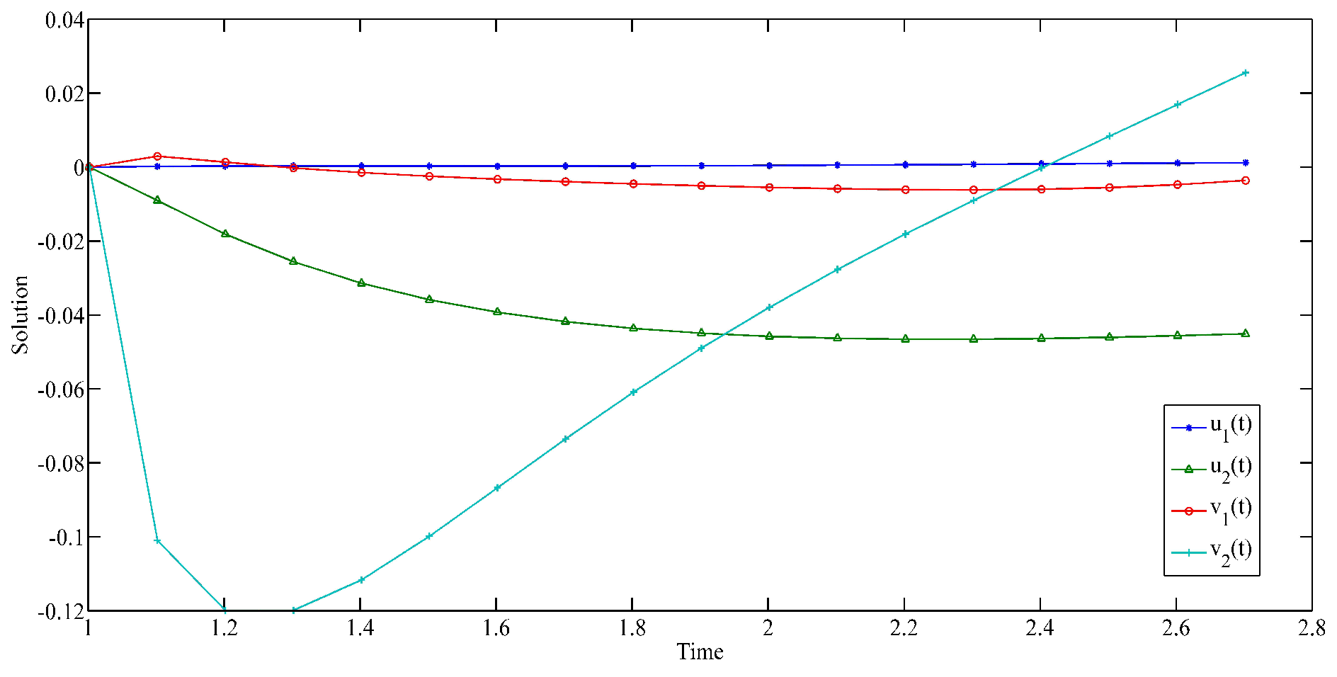
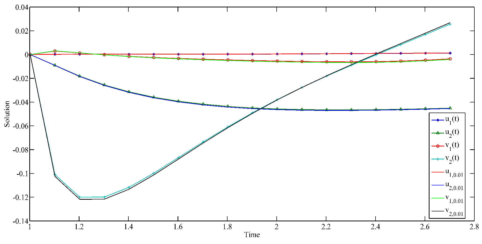
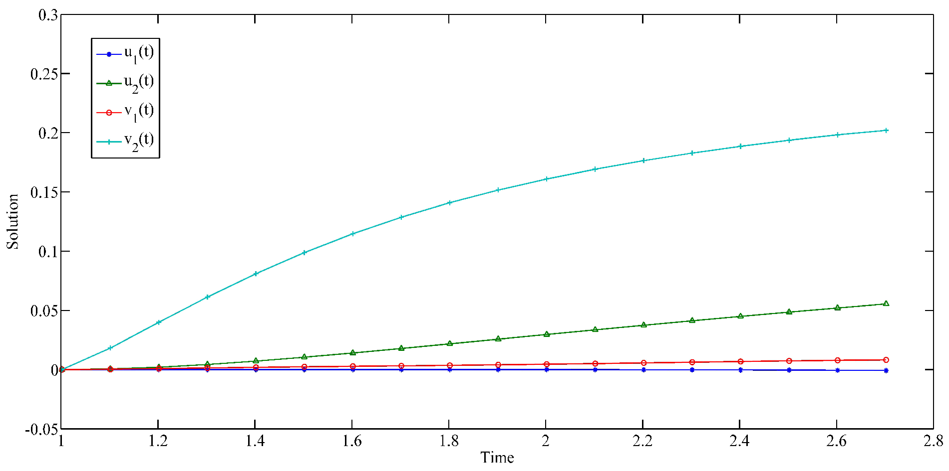
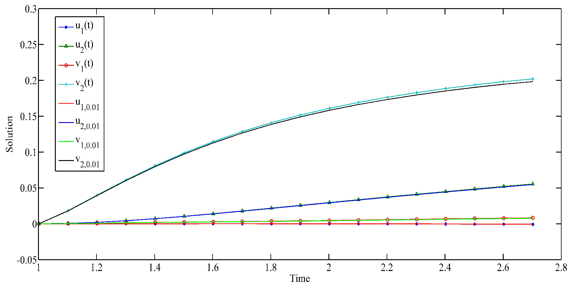
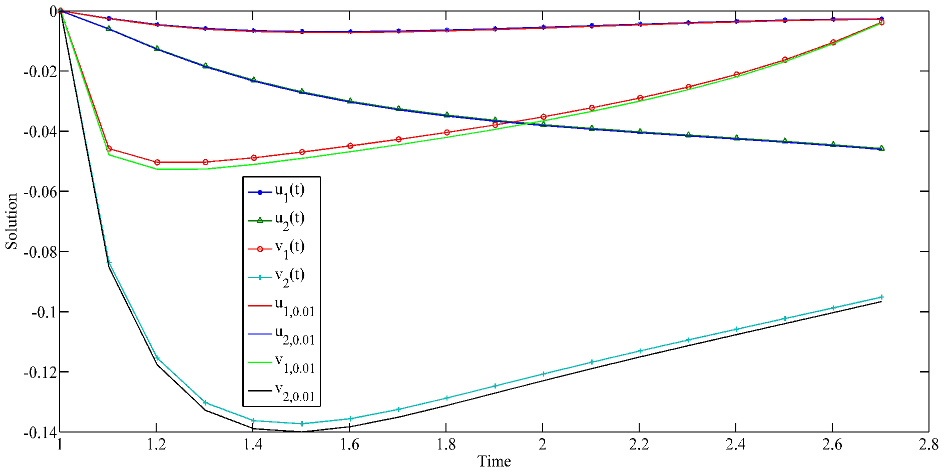
5. Three Examples and Simulations

This section provides three examples to verify the validity and correctness of our main results.

Example 1.

In (1), we take ${\alpha }_1=1.2$, ${\alpha }_2=1.4$, ${\beta }_1=1.8$, ${\beta }_2=1.6$, $p_1=\frac{3}{2}$, $p_2=\frac{7}{4}$, $f_1(t,u_1,u_2)=\frac{2+cos\left(2t\right)}{20}[\frac{5\pi }{4}+arctan\left(u_1\left(t\right)\right)+arctan\left(u_2\left(t\right)\right)]$, $f_2(t,u_1,u_2)=\frac{4+sin\left(2t\right)}{30}[\frac{7\pi }{4}+arctan\left(u_1\left(t\right)\right)+2arctan\left(u_2\left(t\right)\right)]$. By a simple calculation, we have

$$\begin{array}{c}\hfill \frac{\pi }{80}<f_1(t,u_1,u_2)<\frac{27\pi }{80},\frac{\pi }{80}<f_2(t,u_1,u_2)<\frac{13\pi }{24},\end{array}$$

$$\begin{array}{cc}\hfill & |f_1(t,u_1,u_2)-f_1(t,{\overline{u}}_1,{\overline{u}}_2)|<\frac{2+cos\left(2t\right)}{20}\left[\right|u_1-{\overline{u}}_1|+|u_2-{\overline{u}}_2\left|\right],\hfill \\ \hfill & |f_2(t,u_1,u_2)-f_2(t,{\overline{u}}_1,{\overline{u}}_2)|<\frac{4+sin\left(2t\right)}{30}|u_1-{\overline{u}}_1|+\frac{4+sin\left(2t\right)}{15}|u_2-{\overline{u}}_2|.\hfill \end{array}$$

Thus, the conditions $\left({\mathrm{H}}_1\right)$–$\left({\mathrm{H}}_3\right)$ are true. Consequently, $M_1=\frac{27\pi }{80}$, $M_2=\frac{13\pi }{24}$, $\parallel l_{11}{\parallel }_e={\parallel l_{12}\parallel }_e\le \frac{3}{20}$, $\parallel l_{21}{\parallel }_e\le \frac{1}{6}$, $\parallel l_{22}{\parallel }_e\le \frac{1}{3}$. When $p_1=\frac{3}{2}$, $p_2=\frac{7}{4}$, then $q_1=3>2$, $q_2=\frac{7}{3}>2$, and

$$\begin{array}{cc}\hfill & {\kappa }_1=\frac{4(q_1-1)}{\Gamma ({\alpha }_1+{\beta }_1+1)}{\left[\frac{M_1}{\Gamma ({\alpha }_1+1)}\right]}^{q_1-2}\sum _{j=1}^2{\parallel l_{1j}\parallel }_e\le 0.3849<1,\hfill \\ \hfill & {\kappa }_2=\frac{4(q_2-1)}{\Gamma ({\alpha }_2+{\beta }_2+1)}{\left[\frac{M_2}{\Gamma ({\alpha }_2+1)}\right]}^{q_2-2}\sum _{j=1}^2{\parallel l_{2j}\parallel }_e\le 0.4936<1.\hfill \end{array}$$

Thus, $\left({\mathrm{H}}_4\right)$ holds. From Theorems 1 and 2, we claim that system (1) in Example 1 has a unique solution, which is GUH stable.

Remark 2.

In Example 1, ${\alpha }_i$, ${\beta }_i$$(i=1,2)$ are all rational numbers. ${\alpha }_1=1.2$ is close to 1, ${\beta }_1=1.8$ is close to 2, and ${\alpha }_2=1.4$ and ${\beta }_2=1.6$ are close to 1.5. To further verify the correctness of our results and the sensitivity of the numerical simulation to the parameters, we set ${\alpha }_i$ and ${\beta }_i$ close to 2 in Example 2.

Example 2.

In (1), assume ${\alpha }_1=1.9$, ${\alpha }_2=1.95$, ${\beta }_1=1.95$, ${\beta }_2=1.9$, $p_1$, $p_2$, $f_1(t,u_1,u_2)$ and $f_2(t,u_1,u_2)$ are the same as in Example 1. Then, conditions $\left({\mathrm{H}}_1\right)$–$\left({\mathrm{H}}_3\right)$ hold. We simply perform some calculations to obtain

$$\begin{array}{cc}\hfill & {\kappa }_1=\frac{4(q_1-1)}{\Gamma ({\alpha }_1+{\beta }_1+1)}{\left[\frac{M_1}{\Gamma ({\alpha }_1+1)}\right]}^{q_1-2}\sum _{j=1}^2{\parallel l_{1j}\parallel }_e\le 0.0725<1,\hfill \\ \hfill & {\kappa }_2=\frac{4(q_2-1)}{\Gamma ({\alpha }_2+{\beta }_2+1)}{\left[\frac{M_2}{\Gamma ({\alpha }_2+1)}\right]}^{q_2-2}\sum _{j=1}^2{\parallel l_{2j}\parallel }_e\le 0.1337<1.\hfill \end{array}$$

Thus, $\left({\mathrm{H}}_4\right)$ also holds. It follows from Theorems 1 and 2 that system (1) in Example 2 has a unique solution, which is GUH stable.

Remark 3.

In Examples 1 and 2, $p_1$ and $p_2$ are all rational numbers. To further verify the correctness of our results and the sensitivity of the numerical simulation to the parameters, we chose some irrational numbers $p_1$ and $p_2$ satisfying $1<p_1,p_2<2$ in Example 3.

Example 3.

In (1), assume $p_1=\sqrt{3}$, $p_2=\sqrt{2.5}$, ${\alpha }_1$, ${\alpha }_2$, ${\beta }_1$, ${\beta }_2$, $f_1(t,u_1,u_2)$ and $f_2(t,u_1,u_2)$ are the same as in Example 1. Then, conditions $\left({\mathrm{H}}_1\right)$–$\left({\mathrm{H}}_3\right)$ hold. When $p_1=\sqrt{3}$ and $p_2=\sqrt{2.5}$, then $q_1=2.366>2$ and $q_2=2.7208>2$. A simple computation gives that

$$\begin{array}{cc}\hfill & {\kappa }_1=\frac{4(q_1-1)}{\Gamma ({\alpha }_1+{\beta }_1+1)}{\left[\frac{M_1}{\Gamma ({\alpha }_1+1)}\right]}^{q_1-2}\sum _{j=1}^2{\parallel l_{1j}\parallel }_e\le 0.2694<1,\hfill \\ \hfill & {\kappa }_2=\frac{4(q_2-1)}{\Gamma ({\alpha }_2+{\beta }_2+1)}{\left[\frac{M_2}{\Gamma ({\alpha }_2+1)}\right]}^{q_2-2}\sum _{j=1}^2{\parallel l_{2j}\parallel }_e\le 0.7197<1.\hfill \end{array}$$

Thus, $\left({\mathrm{H}}_4\right)$ also holds. We conclude from Theorems 1 and 2 that system (1) in Example 3 has a unique solution, which is GUH stable.

To complete the numerical simulations of Examples 1–3, we present a concise algorithm below. Let $(v_1\left(t\right),v_2\left(t\right))=({ }^H{\mathcal{D}}_{1^{+}}^{{\beta }_1}{u}_1\left(t\right),{ }^H{\mathcal{D}}_{1^{+}}^{{\beta }_2}{u}_2\left(t\right))$; then, system (1) can be rewritten as

$$\begin{array}{c}\hfill \left\{\begin{array}{c}{u}_1\left(t\right)=\frac{1}{\Gamma \left({\beta }_1\right)}\left[{\int }_1^e{\left(\log \frac{e}{s}\right)}^{{\beta }_1-1}{v}_1\left(s\right)\frac{ds}{s}·{\left(\log t\right)}^{{\beta }_1-1}-{\int }_1^t{\left(\log \frac{t}{s}\right)}^{{\beta }_1-1}{v}_1\left(s\right)\frac{ds}{s}\right],\hfill \\ u_2\left(t\right)=\frac{1}{\Gamma \left({\beta }_2\right)}\left[{\int }_1^e{\left(\log \frac{e}{s}\right)}^{{\beta }_2-1}{v}_2\left(s\right)\frac{ds}{s}·{\left(\log t\right)}^{{\beta }_2-1}-{\int }_1^t{\left(\log \frac{t}{s}\right)}^{{\beta }_2-1}{v}_2\left(s\right)\frac{ds}{s}\right],\hfill \\ v_1\left(t\right)=[\frac{1}{\Gamma \left({\alpha }_1\right)}{\int }_1^t{\left(\log \frac{t}{s}\right)}^{{\alpha }_1-1}{f}_1(s,u_1\left(s\right),u_2\left(s\right))\frac{ds}{s}\hfill \\ -\frac{1}{\Gamma \left({\alpha }_1\right)}{\int }_1^e{\left(\log \frac{e}{s}\right)}^{{\alpha }_1-1}{f}_1(s,u_1\left(s\right),u_2\left(s\right))\frac{ds}{s}·{\left(\log t\right)}^{{\alpha }_1-1}{]}^{q_1-1},\hfill \\ v_2\left(t\right)=[\frac{1}{\Gamma \left({\alpha }_2\right)}{\int }_1^t{\left(\log \frac{t}{s}\right)}^{{\alpha }_2-1}{f}_2(s,u_1\left(s\right),u_2\left(s\right))\frac{ds}{s}\hfill \\ -\frac{1}{\Gamma \left({\alpha }_2\right)}{\int }_1^e{\left(\log \frac{e}{s}\right)}^{{\alpha }_2-1}{f}_2(s,u_1\left(s\right),u_2\left(s\right))\frac{ds}{s}·{\left(\log t\right)}^{{\alpha }_2-1}{]}^{q_2-1}.\hfill \end{array}\right.\end{array}$$

(21)

Taking the derivative on both sides of system (21), we get

$$\begin{array}{c}\hfill \left\{\begin{array}{c}\frac{d{u}_1\left(t\right)}{dt}=\frac{{\beta }_1-1}{\Gamma \left({\beta }_1\right)t}\left[{\int }_1^e{\left(\log \frac{e}{s}\right)}^{{\beta }_1-1}{v}_1\left(s\right)\frac{ds}{s}·{\left(\log t\right)}^{{\beta }_1-2}-{\int }_1^t{\left(\log \frac{t}{s}\right)}^{{\beta }_1-2}{v}_1\left(s\right)\frac{ds}{s}\right],\hfill \\ \frac{d{u}_2\left(t\right)}{dt}=\frac{{\beta }_2-1}{\Gamma \left({\beta }_2\right)t}\left[{\int }_1^e{\left(\log \frac{e}{s}\right)}^{{\beta }_2-1}{v}_2\left(s\right)\frac{ds}{s}·{\left(\log t\right)}^{{\beta }_2-2}-{\int }_1^t{\left(\log \frac{t}{s}\right)}^{{\beta }_2-2}{v}_2\left(s\right)\frac{ds}{s}\right],\hfill \\ \frac{d{v}_1\left(t\right)}{dt}=(q_1-1)[\frac{1}{\Gamma \left({\alpha }_1\right)}{\int }_1^t{\left(\log \frac{t}{s}\right)}^{{\alpha }_1-1}{f}_1(s,u_1\left(s\right),u_2\left(s\right))\frac{ds}{s}\hfill \\ -\frac{1}{\Gamma \left({\alpha }_1\right)}{\int }_1^e{\left(\log \frac{e}{s}\right)}^{{\alpha }_1-1}{f}_1(s,u_1\left(s\right),u_2\left(s\right))\frac{ds}{s}·{\left(\log t\right)}^{{\alpha }_1-1}{]}^{q_1-2}\hfill \\ \times \frac{{\alpha }_1-1}{\Gamma \left({\alpha }_1\right)t}[{\int }_1^t{\left(\log \frac{t}{s}\right)}^{{\alpha }_1-2}{f}_1(s,u_1\left(s\right),u_2\left(s\right))\frac{ds}{s}\hfill \\ -{\int }_1^e{\left(\log \frac{e}{s}\right)}^{{\alpha }_1-1}{f}_1(s,u_1\left(s\right),u_2\left(s\right))\frac{ds}{s}·{\left(\log t\right)}^{{\alpha }_1-2}],\hfill \\ \frac{d{v}_2\left(t\right)}{dt}=(q_2-1)[\frac{1}{\Gamma \left({\alpha }_2\right)}{\int }_1^t{\left(\log \frac{t}{s}\right)}^{{\alpha }_2-1}{f}_2(s,u_1\left(s\right),u_2\left(s\right))\frac{ds}{s}\hfill \\ -\frac{1}{\Gamma \left({\alpha }_2\right)}{\int }_1^e{\left(\log \frac{e}{s}\right)}^{{\alpha }_2-1}{f}_2(s,u_1\left(s\right),u_2\left(s\right))\frac{ds}{s}·{\left(\log t\right)}^{{\alpha }_2-1}{]}^{q_2-2}\hfill \\ \times \frac{{\alpha }_2-1}{\Gamma \left({\alpha }_2\right)t}[{\int }_1^t{\left(\log \frac{t}{s}\right)}^{{\alpha }_2-2}{f}_2(s,u_1\left(s\right),u_2\left(s\right))\frac{ds}{s}\hfill \\ -{\int }_1^e{\left(\log \frac{e}{s}\right)}^{{\alpha }_2-1}{f}_2(s,u_1\left(s\right),u_2\left(s\right))\frac{ds}{s}·{\left(\log t\right)}^{{\alpha }_2-2}].\hfill \end{array}\right.\end{array}$$

(22)

We can use the appropriate ODE toolbox in MATLAB to complete numerical simulations of (22). Based on the above analysis, we employ the ODE113 toolbox in MATLAB R2017b on the three examples to present numerical simulations of their solutions and GUH stability. The simulation diagrams are shown in Figure 1, Figure 2, Figure 3, Figure 4, Figure 5 and Figure 6.

6. Conclusions

The Hadamard fractional derivative and integral are important parts of fractional calculus which have been widely used in engineering, biology, neural networks, control theory, and so on. Compared with a single Hadamard fractional system, Hadamard fractional coupling systems have a more complex structure and a wide range of applications. As far as we know, there are no works dealing with nonlinear Hadamard fractional coupling Laplacian systems with periodic boundary value conditions. So, we investigated system (1) to fill this gap. In this article, we consider a class of nonlinear Hadamard fractional coupling $(p_1$, $p_2)$-Laplacian systems with periodic boundary value conditions. Based on nonlinear analysis methods and contraction mapping principle, we obtain some new and easily verifiable sufficient criteria of the existence, uniqueness and GUH stability of solutions of system (1). Examples 1–3 and their simulations demonstrate the correctness and availability of our main results. Meanwhile, Figure 2, Figure 4 and Figure 6 also indicate that the solution of (1) is sensitive and dependent on parameters $p_i$, ${\alpha }_i$ and ${\beta }_i$, $i=1,2.$ In addition, inspired by recently published papers [9,47,48], we will investigate the Lyapunov stability of fractional differential equations, the coincidence theory of fractional differential equations, and fractional differential equations involving fractional derivative impulses in the future.

References

1. Hadamard, J. Essai sur l’étude des fonctions données par leur développment de Taylor. J. Math. Pures Appl. 1892, 8, 101–186. [Google Scholar]
2. Ahmad, B.; Alsaedi, A.; Ntouyas, S.; Tariboon, J.J. Hadamard-Type Fractional Differential Equations, Inclusions and Inequalities; Springer: Berlin/Heidelberg, Germany, 2017. [Google Scholar]
3. Kilbas, A.; Srivastava, H.M.; Trujillo, J.J. Theory and Applications of Fractional Differential Equations; Elsevier: Amsterdam, The Netherlands, 2006. [Google Scholar]
4. Baleanu, D.; Diethelm, K.; Scalas, E.; Trujillo, J.J. Fractional Calculus: Models and Numerical Methods; World Scientific: Singapore, 2012. [Google Scholar]
5. Miller, K.; Ross, B. An introduction to the Fractional Calculus and Differential Equations; Wiley: New York, NY, USA, 1993. [Google Scholar]
6. Zhou, Y. Basic Theory of Fractional Differential Equations; World Scientific: Singapore, 2014. [Google Scholar]
7. Aljoudi, S.; Ahmad, B.; Nieto, J.; Alsaedi, A. A coupled system of Hadamard type sequential fractional differential equations with coupled strip conditions. Chaos Soliton. Fract. 2016, 91, 39–46. [Google Scholar] [CrossRef]
8. Benchohra, M.; Bouriah, S.; Graef, J. Boundary value problems for nonlinear implicit Caputo-Hadamard-type fractional differential equations with impulses. Mediterr. J. Math. 2017, 14, 206. [Google Scholar] [CrossRef]
9. Huang, H.; Zhao, K.; Liu, X. On solvability of BVP for a coupled Hadamard fractional systems involving fractional derivative impulses. AIMS Math. 2022, 7, 19221–19236. [Google Scholar] [CrossRef]
10. Mouy, M.; Boulares, H.; Alshammari, S.; Alshammari, M.; Laskri, Y.; Mohammed, W.W. On averaging principle for Caputo-Hadamard fractional stochastic differential pantograph equation. Fractal Fract. 2023, 7, 31. [Google Scholar] [CrossRef]
11. Ortigueira, M.; Bohannan, G. Fractional scale calculus: Hadamard vs. Liouville. Fractal Fract. 2023, 7, 296. [Google Scholar] [CrossRef]
12. Zhao, K. Existence and UH-stability of integral boundary problem for a class of nonlinear higher-order Hadamard fractional Langevin equation via Mittag–Leffler functions. Filomat 2023, 37, 1053–1063. [Google Scholar] [CrossRef]
13. Nyamoradi, N.; Ahmad, B. Hadamard fractional differential equations on an unbounded domain with integro-initial conditions. Qual. Theor. Dyn. Syst. 2024, 23, 183. [Google Scholar] [CrossRef]
14. Alruwaily, Y.; Venkatachalam, K.; El-hady, E. On some impulsive fractional integro-differential equation with anti-periodic conditions. Fractal Fract. 2024, 8, 219. [Google Scholar] [CrossRef]
15. Hammad, H.; Aydi, H.; Kattan, D. Integro-differential equations implicated with Caputo-Hadamard derivatives under nonlocal boundary constraints. Phys. Scr. 2024, 99, 025207. [Google Scholar] [CrossRef]
16. Kassim, M. Convergence to logarithmic-type functions of solutions of fractional systems with Caputo-Hadamard and Hadamard fractional derivatives. Fract. Calc. Appl. Anal. 2024, 27, 281–318. [Google Scholar] [CrossRef]
17. Zhang, K.; Xu, J. Solvability for a system of Hadamard-type hybrid fractional differential inclusions. Demonstr. Math. 2023, 56, 20220226. [Google Scholar] [CrossRef]
18. Ciftci, C.; Deren, F. Analysis of p-Laplacian Hadamard fractional boundary value problems with the derivative term involved in the nonlinear term. Math. Method. Appl. Sci. 2023, 46, 8945–8955. [Google Scholar] [CrossRef]
19. Rafeeq, A.; Thabet, S.; Mohammed, M.; Kedim, I.; Vivas-Cortez, M. On Caputo-Hadamard fractional pantograph problem of two different orders with Dirichlet boundary conditions. Alex. Eng. J. 2024, 86, 386–398. [Google Scholar] [CrossRef]
20. Leibenson, L. General problem of the movement of a compressible uid in a porous medium. Izv. Akad. Nauk Kirg. SSR Ser. Biol. Nauk 1983, 9, 7–10. [Google Scholar]
21. Zhao, K. Solvability, Approximation and Stability of Periodic Boundary Value Problem for a Nonlinear Hadamard Fractional Differential Equation with p-Laplacian. Axioms 2023, 12, 733. [Google Scholar] [CrossRef]
22. Zhao, K. Study on the stability and its simulation algorithm of a nonlinear impulsive ABC-fractional coupled system with a Laplacian operator via F-contractive mapping. Adv. Contin. Discret. Models 2024, 2024, 5. [Google Scholar] [CrossRef]
23. Rao, S.; Ahmadini, A. Multiple positive solutions for system of mixed Hadamard fractional boundary value problems with (p1,p2)-Laplacian operator. AIMS Math. 2023, 8, 14767–14791. [Google Scholar] [CrossRef]
24. Alkhazzan, A.; Al-Sadi, W.; Wattanakejorn, V.; Khan, H.; Sitthiwirattham, T.; Etemad, S.; Rezapour, S. A new study on the existence and stability to a system of coupled higher-order nonlinear BVP of hybrid FDEs under the p-Laplacian operator. AIMS Math. 2022, 7, 14187–14207. [Google Scholar] [CrossRef]
25. Khan, H.; Chen, W.; Sun, H. Analysis of positive solution and Hyers-Ulam stability for a class of singular fractional differential equations with p-Laplacian in Banach space. Math. Methods Appl. Sci. 2018, 41, 3430–3440. [Google Scholar] [CrossRef]
26. Li, S.; Zhang, Z.; Jiang, W. Multiple positive solutions for four-point boundary value problem of fractional delay differential equations with p-Laplacian operator. Appl. Numer. Math. 2021, 165, 348–356. [Google Scholar] [CrossRef]
27. Ulam, S. A Collection of Mathematical Problems. Interscience Tracts in Pure and Applied Mathmatics; Interscience: New York, NY, USA, 1906. [Google Scholar]
28. Hyers, D. On the stability of the linear functional equation. Proc. Natl. Acad. Sci. USA 1941, 27, 2222–2240. [Google Scholar] [CrossRef] [PubMed]
29. Ali, Z.; Zada, A.; Shah, K. On Ulam’s stability for a coupled systems of nonlinear implicit fractional differential equations. Bull. Malays. Math. Sci. Soc. 2019, 42, 2681–2699. [Google Scholar] [CrossRef]
30. Ahmad, M.; Zada, A.; Ghaderi, M.; George, R.; Rezapour, S. On the existence and stability of a neutral stochastic fractional differential system. Fractal Fract. 2022, 6, 203. [Google Scholar] [CrossRef]
31. Ahmadova, A.; Mahmudov, N. Ulam-Hyers stability of Caputo type fractional stochastic neutral differential equations. Stat. Probabil. Lett. 2021, 168, 108949. [Google Scholar] [CrossRef]
32. Li, M.; Wang, J. Existence results and Ulam type stability for conformable fractional oscillating system with pure delay. Chaos Soliton. Fract. 2022, 161, 112317. [Google Scholar] [CrossRef]
33. Zhao, K. Stability of a nonlinear Langevin system of ML-Type fractional derivative affected by time-varying delays and differential feedback control. Fractal Fract. 2022, 6, 725. [Google Scholar] [CrossRef]
34. Rizwan, R.; Liu, F.; Zheng, Z.; Park, C.; Paokanta, S. Existence theory and Ulam’s stabilities for switched coupled system of implicit impulsive fractional order Langevin equations. Bound. Value Probl. 2023, 2023, 115. [Google Scholar] [CrossRef]
35. Priyadharsini, J.; Balasubramaniam, P. Hyers-Ulam stability result for hilfer fractional integrodifferential stochastic equations with fractional noises and non-instantaneous impulses. Evol. Equ. Control. Theory 2024, 13, 173–193. [Google Scholar] [CrossRef]
36. Thabet, S.; Vivas-Cortez, M.; Kedim, I.; Samei, M.E.; Ayari, M.I. Solvability of a ϱ-Hilfer fractional snap dynamic system on unbounded domains. Fractal Fract. 2023, 7, 607. [Google Scholar] [CrossRef]
37. Shah, S.; Rizwan, R.; Xia, Y.; Zada, A. Existence, uniqueness, and stability analysis of fractional Langevin equations with anti-periodic boundary conditions. Math. Methods Appl. Sci. 2023, 46, 17941–17961. [Google Scholar] [CrossRef]
38. Zhao, K. Solvability and GUH-stability of a nonlinear CF-fractional coupled Laplacian equations. AIMS Math. 2023, 8, 13351–13367. [Google Scholar] [CrossRef]
39. Alam, M.; Khalid, K. Analysis of q-fractional coupled implicit systems involving the nonlocal Riemann–Liouville and Erdelyi-Kober q-fractional integral conditions. Math. Methods Appl. Sci. 2023, 46, 12711–12734. [Google Scholar] [CrossRef]
40. Khan, T.; Markarian, C.; Fachkha, C. Stability analysis of new generalized mean-square stochastic fractional differential equations and their applications in technology. AIMS Math. 2023, 8, 27840–27856. [Google Scholar] [CrossRef]
41. Kiskinov, H.; Milev, M.; Cholakov, S.; Zahariev, A. Fundamental matrix, integral representation and stability analysis of the solutions of neutral fractional systems with derivatives in the Riemann–Liouville sense. Fractal Fract. 2024, 8, 195. [Google Scholar] [CrossRef]
42. Bensassa, K.; Dahmani, Z.; Rakah, M.; Sarikaya, M.Z. Beam deflection coupled systems of fractional differential equations: Existence of solutions, Ulam-Hyers stability and travelling waves. Anal. Math. Phys. 2024, 14, 29. [Google Scholar] [CrossRef]
43. Zhao, K. Generalized UH-stability of a nonlinear fractional coupling (p1,p2)-Laplacian system concerned with nonsingular Atangana-Baleanu fractional calculus. J. Inequal. Appl. 2023, 2023, 96. [Google Scholar] [CrossRef]
44. Shah, K.; Sarwar, M.; Abdeljawad, T.; Shafiullah. Sufficient criteria for the existence of solution to nonlinear fractal-fractional order coupled system with coupled integral boundary conditions. J. Appl. Math. Comput. 2024, 70, 1771–1785. [Google Scholar] [CrossRef]
45. Zhang, L.; Liu, X.; Jia, M.; Yu, Z. Piecewise conformable fractional impulsive differential system with delay: Existence, uniqueness and Ulam stability. J. Appl. Math. Comput. 2024, 70, 1543–1570. [Google Scholar] [CrossRef]
46. Guo, D.; Lakshmikantham, V. Nonlinear Problems in Abstract Cone; Academic Press: Orlando, FL, USA, 1988. [Google Scholar]
47. Zhao, K.; Liu, J.; Lv, X. A unified approach to solvability and stability of multipoint BVPs for Langevin and Sturm–Liouville equations with CH–fractional derivatives and impulses via coincidence theory. Fractal Fract. 2024, 8, 111. [Google Scholar] [CrossRef]
48. Zhao, K. Global stability of a novel nonlinear diffusion online game addiction model with unsustainable control. AIMS Math. 2022, 7, 20752–20766. [Google Scholar] [CrossRef]
Figure 1. Numerical simulation of solutions in Example 1.
Symmetry 16 00774 g001
Figure 2. Numerical simulation of GUH stability with ϵ = 0.01 in Example 1.
Symmetry 16 00774 g002
Figure 3. Numerical simulation of solutions in Example 2.
Symmetry 16 00774 g003
Figure 4. Numerical simulation of GUH stability with ϵ = 0.01 in Example 2.
Symmetry 16 00774 g004
Figure 5. Numerical simulation of solutions in Example 3.
Symmetry 16 00774 g005
Figure 6. Numerical simulation of GUH stability with ϵ = 0.01 in Example 3.
Symmetry 16 00774 g006
Disclaimer/Publisher’s Note: The statements, opinions and data contained in all publications are solely those of the individual author(s) and contributor(s) and not of MDPI and/or the editor(s). MDPI and/or the editor(s) disclaim responsibility for any injury to people or property resulting from any ideas, methods, instructions or products referred to in the content.