Article

Assorted Spatial Optical Dynamics of a Generalized Fractional Quadruple Nematic Liquid Crystal System in Non-Local Media

by
Mohammad A. Al Zubi
1,
Kallekh Afef
2 and
Emad A. Az-Zo’bi
3,*
1
Mechanical Engineering Department, Yarmouk University, Irbid 21163, Jordan
2
Department of Mathematics, College of Science & Arts at Mahayil, King Khalid University, Mohail Asser, Abha 61413, Saudi Arabia
3
Department of Mathematics and Statistics, Faculty of Science, Mutah University, P.O. Box 7, Al-Karak 61710, Jordan
*
Author to whom correspondence should be addressed.
Symmetry 2024, 16(6), 778; https://doi.org/10.3390/sym16060778
Submission received: 22 May 2024 / Revised: 11 June 2024 / Accepted: 12 June 2024 / Published: 20 June 2024

Abstract

:
Nematicons upgrade the recognition of light localization in the reorientation of non-local media. the current research employs a powerful integral scheme using a different procedure, namely, the modified simple equation method (MSEM), to analyze nematicons in liquid crystals from the controlling model. The expanded MSEM is investigated to enlarge the applicability of the standard one. The suggested expansion depends on merging the MSEM and the ansatz method. The new generalized nonlinear n-times quadruple power law is included. With the aid of the symbolic computational package Mathematica, new explicit complex hyperbolic, periodic, and more exact spatial soliton solutions are derived. Moreover, the related existence constraints are obtained. To show the dynamical properties of some of the obtained nematicons, three-dimensional profiles with corresponding contours are depicted with the choice of appropriate values of arbitrary parameters. The fractional impacts in various applicable senses are analyzed to investigate the generality of the considered model.

1. Introduction

Nonlinear functional problems, including differentials, have wide areas of applications in various fields of science, engineering, medicine, statistics, and artificial intelligence [1,2,3,4]; see also the references included therein. They modeled many real-life phenomena. Therefore, to explain these phenomena and draw conclusions in scientific and practical ways, applied scientists have devoted attention to solving these models. For this purpose, a number of analytic, series-expansion, and numerical schemes were developed, for instance, the improved BPNN method [5], the Adomian decomposition method [6], the variational iteration method [7], the differential transform method [8], the residual power series method [9], the Lie symmetry approach [10], the generalized auxiliary equation method [11], the generalized Riccati equation mapping method [12], the improved Bernoulli sub-equation function technique [13], the G G 2 and F-expansion methods [14], the modified Kudryashov procedure [15], the Sardar sub-ODE method [16], the generalized exponential rational function method [17], and the extended rational sine–cosine, sinh–cosh and sinh–Gordon equation expansion methods [18].
Recently, spatial optical solitons in the applied theory of nonlinear optics, particularly in metasurfaces, metamaterials, liquid crystals, etc., have received considerable attention. In the field of liquid crystals, nematicons, first introduced by Alberucci and Assanto to describe spatial solitons produced by a special type of optical nonlinearity found in nematic liquid crystals, are a class of dielectric media, utilized in processing electronic, thermal, and photo refractive phenomena [19,20]. Nematicons present a noteworthy platform for exploring optical processing and switching techniques depending on self and cross localization of light. While the observed effects exhibit inherent slowness, the potential for a faster response can be obtained using other materials or geometries, leading the way towards applied optical communication.
The formal dimensionless soliton dynamics in liquid crystals are given using the coupled system of NPDEs [21]:
i q t + α 1 2 q x 2 + α 2 p q = 0 ,
α 3 2 p x 2 + α 4 p + α 5 H q 2 = 0 .
The dependent variables q x , t and p x , t symbolize the wave profile and the tilt angle of the liquid crystal molecule, respectively. In Equation (1), i = 1 , and i q t describes the temporal evolution of nematicons, while 2 q x 2 stands for the group velocity dispersion (GVD). The nonlinear operator H includes the Kerr, power, parabolic, and dual-power types of nonlinearity. Moreover, α ’s are assumed to be the parameters.
Many researchers have studied Equations (1) and (2), with the abovementioned types of nonlinearity. Some of these attempts were as follows: the extended sinh–Gordon equation expansion method [22], the exp ϕ ξ -expansion method [23], the extended trial equation method [24], the extended simplest equation technique, the modified Khater and modified Kudryashov methods [25], the tan ϕ / 2 -expansion method [26], the generalized exponential rational function method [27], and the modified extended tangent hyperbolic function method [28]. The conservation laws of the liquid crystal model were derived in [29,30].
A novel generalized nematic liquid crystal model, with Equations (1) and (2) and the nonlinear nth-quadruple power non-Kerr law, is given by
H z = C 0 + C 1 z n + C 2 z 2 n + C 3 z 3 n + C 4 z 4 n ,
where n is a nonzero integer, and C i ’s are assumed to be scalars coefficients. Continuing our previous analysis [31], we analytically processed the liquid crystal governing model, Equations (1) and (2), with the quadruple power of nonlinearity in Equation (3), applying the MSEM and its expansion.
The outline of this article is as follows: Section 2 includes a brief discussion of the modified simple equation scheme and its expansion for general dimensionless NPDE. Section 3 and Section 4 present an analytic treatment of the considered model with formal closed nematicons. In Section 5, the dynamics of some of the obtained nematicons are depicted. To cover more general cases and due to the significance of fractional calculus, the impact of the modified Riemann–Liouville, beta, and modified conformable fractional derivatives have been customized graphically in Section 6. Finally, a concise discussion and the conclusions are provided.

2. Outline of the Methodology

The main steps of the considered scheme, the MSEM, are demonstrated to process the formal dimensionless nonlinear evolution model given by
F ( q , q t , q x , 2 q t 2 , 2 q x 2 , 2 q t x , ) = 0 ,
where F is a polynomial in q ( x , t ) , with its total space x and time t as the partial derivatives.
Step 1. 
We proceed with the wave transformation
q ( x , t ) = u ( η ) , η = β ( x ± ν t ) .
Equation (4) can be reduced to the nonlinear ordinary differential equation (NODE)
G q ( η ) , q ( η ) , q ( η ) , = 0 ,
where q η = d q d η , q η = d 2 q d η 2 , etc. G is a polynomial of q η and all its derivatives.
Step 2. 
The MSEM is performed by assuming the solution of Equation (6) as
u ( η ) = i = 0 N A i ϕ ( η ) ϕ ( η ) i , A N 0 ,
where A i ( i = 0 , 1 , , m ) are constants to be found later. ϕ ( η ) is an undetermined real-valued function to be calculated later.
Step 3. 
We compute the positive integer N by implementing the homogeneous balance between terms containing the highest order derivative and nonlinearity in the completely integrated version of Equation (6).
Step 4. 
We replace the assumed ansatz in Equation (7) with the value of N in the previous step and its essential derivatives in Equation (6). As a result, a polynomial of ϕ i η , i = 0 , 1 , 2 , , is obtained. We gather the terms of the same power of ϕ i η and make them vanish for each i, and we deduce a mixed algebraic–differential system. By solving this system, the values of ϕ η and A i ’s are derived. To completely determine the exact solution of Equation (4), we place the results into Equation (5).
Consequently, the expansion of the modified simple equation algorithm is based on replacing the unknown function ϕ η with a helpful hyperbolic or trigonometric function. Depending on this assumption, the mixed algebraic–differential system should result in some algebraic–functional equations. To clarify, collecting the coefficients of the linearly independent expressions in the obtained equation and equating to zero, a free-functional algebraic system will be obtained. The procedure depends on the assumed ϕ as mentioned in [32]. By solving this system for the undetermined parameters, namely the constraints for the solution’s existence, and making the backward substitution, the closed form solitons can be be derived.
The modified simple equation scheme has been successfully employed to analytically treat the Fitzhugh–Nagumo and Sharma–Tasso–Olver equations [33], the dimensionless modified KdV and reaction–diffusion equations [34], generalized Zakharov–Kuznetsov–Benjamin–Bona–Mahon and non-commutative Burger equations [35], the van der Waals p-system [36], the higher dimensional Fokas equation [37], the nonlinear Klein–Gordon–Zakharov, generalized Davey–Stewartson, Davey–Stewartson, and generalized Zakharov equations [38], the nonlocal Ito integro-differential equation [39], some nonlinear Schrödinger-type equations [40,41], the shallow-water waves equation [42], the higher dimensional Calogero–Bogoyavlenskii–Schiff and Jimbo–Miwa equations [43], and the modified Fornberg–Whitham equation [44].

3. Mathematical Treatment

Following the procedure in the previous section with application to the coupled system in Equations (1) and (2), subject the to non-Kerr operator in Equation (3), we consider the traveling-wave transform η = β ( x ν t ) and the solutions of the form
q ( x , t ) = u ( η ) e i κ x + ω t + θ 0 ,
p ( x , t ) = v ( η ) ,
where ν is the propagation wave speed, and κ , ω , and θ 0 represent the soliton frequency, the wave number of the soliton, and the phase constant, respectively. Substituting Equations (8) and (9) into Equations (1) and (2) and separating the obtained NODEs into real and imaginary parts, we obtain
α 1 β 2 u ( η ) α 1 κ 2 α 2 v ( η ) + ω u ( η ) = 0 ,
α 3 β 2 v ( η ) + α 4 v ( η ) + α 5 H u 2 ( η ) = 0 ,
and
2 α 1 β κ β ν u ( η ) = 0 .
The imaginary component in Equation (12) leads to the constraint condition regarding the soliton speed
ν = 2 α 1 κ .
Thus, Equations (10) and (11) are deducted to the following completely integrable system of NODEs:
α 1 β 2 u ( η ) α 1 κ 2 α 2 v ( η ) + ω u ( η ) = 0 ,
α 3 β 2 v ( η ) + α 4 v ( η ) + α 5 C 0 + C 1 u 2 n + C 2 u 4 n + C 3 u 6 n + C 4 u 8 n = 0 .
We define the following new dependent variables
u ( η ) = U ( η ) 1 2 n , v ( η ) = V ( η ) 2
to transform Equations (14) and (15) into
4 n 2 α 1 κ 2 + ω α 2 V 2 U 2 + α 1 β 2 ( 2 n 1 ) U 2 2 n α 1 β 2 U U = 0 ,
α 4 V 2 + 2 α 3 β 2 V V + V 2 + α 5 C 0 + C 1 U + C 2 U 2 + C 3 U 3 + C 4 U 4 = 0 .
Applying the homogeneous balance principle between the terms containing the highest order derivatives U U , V V and nonlinear terms V 2 U 2 , U 4 in Equations (17) and (18), respectively, results in the following system:
2 M + 2 = 2 M + 2 N , 2 N + 2 = 4 M .
This implies that N = M = 1 , where M and N represent the corresponding balance integers of U and V, respectively.
Therefore, the formal solutions of Equations (17) and (18) are
U η = A 0 + A 1 ϕ η ϕ η , V η = B 0 + B 1 ϕ η ϕ η .
In the next section, exact nematicons for our model are derived.

4. Application

To complete the derivation of the closed-form soliton solutions, we substitute Equation (19) into Equations (17) and (18), collect the coefficients of ϕ i ( η ) , i = 0 , 1 , 2 , 3 , 4 , with the same power in both obtained sets of differential–algebraic systems, make them vanish, and we obtain
4 A 0 2 n 2 α 1 κ 2 α 2 B 0 2 + ω = 0 ,
4 α 2 B 1 2 n 2 + α 1 β 2 ( 2 n + 1 ) = 0 ,
2 n ϕ ( η ) α 1 A 0 β 2 + 2 α 2 B 1 n A 1 B 0 + A 0 B 1 α 1 A 1 β 2 ( n + 1 ) ϕ ( η ) = 0 ,
2 A 0 n A 1 α 1 β 2 ϕ ( 3 ) ( η ) 4 n ϕ ( η ) α 1 κ 2 α 2 B 0 2 + ω + 4 α 2 A 0 B 0 B 1 n ϕ ( η ) = 0 ,
4 n 2 A 0 2 B 1 2 α 2 ϕ η 2 + 2 n A 0 A 1 ϕ η 8 n B 0 B 1 α 2 ϕ η + 3 β 2 α 1 ϕ η + A 1 2 × 4 n 2 ω + κ 2 α 1 B 0 2 α 2 ϕ η 2 + 1 + 2 n β 2 α 1 ϕ η 2 2 n β 2 α 1 ϕ η ϕ 3 η = 0 ,
α 5 A 0 A 0 A 0 A 0 C 4 + C 3 + C 2 + C 1 + C 0 + α 4 B 0 2 = 0 ,
α 5 A 1 4 C 4 + 6 α 3 β 2 B 1 2 = 0 ,
α 5 A 1 3 4 A 0 C 4 + C 3 ϕ ( η ) 10 α 3 β 2 B 1 2 ϕ ( η ) + 4 α 3 β 2 B 0 B 1 ϕ ( η ) = 0 ,
α 5 A 1 A 0 4 A 0 2 C 4 + 3 A 0 C 3 + 2 C 2 + C 1 ϕ ( η ) + 2 B 0 B 1 α 3 β 2 ϕ ( 3 ) ( η ) + α 4 ϕ ( η ) = 0 ,
α 5 A 1 2 3 A 0 2 A 0 C 4 + C 3 + C 2 ϕ ( η ) 2 6 α 3 β 2 B 0 B 1 ϕ ( η ) ϕ ( η ) + B 1 2 2 α 3 β 2 ϕ ( η ) 2 + ϕ ( 3 ) ( η ) ϕ ( η ) + α 4 ϕ ( η ) 2 = 0 .
The nontrivial solutions with different structures and corresponding existence constraints are listed as follows:
  • Case 1. The unknown function ϕ can be determined directly by solving the linear ordinary differential equations that appear in Equation (22), Equation (23), Equation (27), or Equation (28). With the first choice, we obtain
    κ = κ 0 , B 1 = B 1 0 , ω = α 1 κ 2 α 2 α 5 C 0 n 2 α 4 ( n + 1 ) 2 , β = 2 B 1 n α 2 α 1 + 2 α 1 n , A 0 = 2 C 0 ( 2 n + 1 ) 4 α 2 α 3 α 5 C 0 ( 2 n + 1 ) n 2 + α 1 α 4 2 ( n + 1 ) 2 α 1 α 4 2 C 1 ( n + 1 ) 3 , A 1 = 2 B 1 C 0 n 4 α 2 α 3 α 5 C 0 ( 2 n + 1 ) n 2 + α 1 α 4 2 ( n + 1 ) 2 α 1 α 4 2 C 1 ( n + 1 ) 3 α 5 C 0 n 2 α 4 ( n + 1 ) 2 , B 0 = n α 5 C 0 α 4 n + 1 , C 2 = α 1 α 4 2 C 1 2 ( n + 1 ) 2 8 α 2 α 3 α 5 C 0 ( 7 n + 5 ) n 2 + α 1 α 4 2 ( n + 1 ) 2 4 C 0 4 α 2 α 3 α 5 C 0 ( 2 n + 1 ) n 2 + α 1 α 4 2 ( n + 1 ) 2 2 , C 3 = α 1 2 α 2 α 3 α 4 4 α 5 C 1 3 n 2 ( n + 1 ) 5 ( 12 n + 7 ) C 0 ( 2 n + 1 ) 4 α 2 α 3 α 5 C 0 ( 2 n + 1 ) n 2 + α 1 α 4 2 ( n + 1 ) 2 3 , C 4 = 3 α 1 3 α 2 α 3 α 4 6 α 5 C 1 4 n 2 ( n + 1 ) 8 2 C 0 2 ( 2 n + 1 ) 4 α 2 α 3 α 5 C 0 ( 2 n + 1 ) n 2 + α 1 α 4 2 ( n + 1 ) 2 4 ,
    and
    ϕ ( η ) = γ 2 ( 2 n + 1 ) α 5 C 0 α 4 B 1 γ 1 ( n + 1 ) exp η ( 2 n + 1 ) α 5 C 0 α 4 B 1 ( n + 1 ) ( 2 n + 1 ) α 5 C 0 α 4 ,
    where γ 1 , and γ 2 0 are the constants of integration. For the parameters set in Equations (30) and (31), the closed-form spatial soliton solutions of our model will be
    q 1 ( x , t ) = 2 1 2 n e i ψ ( η ) γ 2 C 0 ( 2 n + 1 ) 2 α 5 C 0 α 4 4 α 2 α 3 α 5 C 0 ( 2 n + 1 ) n 2 + α 1 α 4 2 ( n + 1 ) 2 α 1 α 4 2 C 1 ( n + 1 ) 3 γ 2 ( 2 n + 1 ) α 5 C 0 α 4 B 1 γ 1 ( n + 1 ) exp η ( 2 n + 1 ) α 5 C 0 α 4 B 1 ( n + 1 ) 1 2 n ,
    p 1 ( x , t ) = B 1 γ 1 ( n + 1 ) 2 α 5 C 0 α 4 α 5 γ 2 C 0 n ( 2 n + 1 ) exp η ( 2 n + 1 ) α 5 C 0 α 4 B 1 ( n + 1 ) α 4 2 ( n + 1 ) 2 γ 2 ( 2 n + 1 ) α 5 C 0 α 4 exp η ( 2 n + 1 ) α 5 C 0 α 4 B 1 ( n + 1 ) B 1 γ 1 ( n + 1 ) 2 ,
    with
    η = 2 B 1 n α 2 α 1 + 2 α 1 n 2 α 1 κ t + x , ψ = α 2 α 5 C 0 n 2 t α 4 ( n + 1 ) 2 + θ 0 α 1 κ 2 t κ x .
  • Case 2. The MSEM provides the possibility of merging two linear differential equations with different orders. In our case, Equation (22) and Equation (28) provide
    ϕ ( η ) = α 1 β 2 ( n + 1 ) ϕ ( η ) 4 α 2 B 0 B 1 n 2 = 2 α 3 β 2 B 0 B 1 ϕ ( 3 ) ( η ) α 5 A 1 C 1 + 2 α 4 B 0 B 1 .
Subsequently,
ϕ ( 3 ) ( η ) ϕ ( η ) = α 1 ( n + 1 ) α 5 A 1 C 1 + 2 α 4 B 0 B 1 8 α 2 α 3 B 0 2 B 1 2 n 2 .
Upon integrating Equation (36), we obtain
ϕ ( η ) = γ 1 exp α 1 η ( n + 1 ) α 5 A 1 C 1 + 2 α 4 B 0 B 1 8 α 2 α 3 B 0 2 B 1 2 n 2 .
Consequently, and with Equation (35), we obtain
ϕ ( η ) = γ 1 α 1 β 2 + α 1 β 2 n exp α 1 η ( n + 1 ) α 5 A 1 C 1 + 2 α 4 B 0 B 1 8 α 2 α 3 B 0 2 B 1 2 n 2 4 α 2 B 0 B 1 n 2 .
That yields
ϕ ( η ) = γ 2 2 α 3 β 2 B 0 B 1 γ 1 exp α 1 η ( n + 1 ) α 5 A 1 C 1 + 2 α 4 B 0 B 1 8 α 2 α 3 B 0 2 B 1 2 n 2 α 5 A 1 C 1 + 2 α 4 B 0 B 1 ,
where γ 1 , and γ 2 are the constants of integration. The undetermined parameters, as well as the constraints depending on the obtained ϕ , are as follows:
κ = κ 0 , β = β 0 , A 0 = 0 , ω = α 1 κ 2 α 2 α 5 C 0 n 2 α 4 ( n + 1 ) 2 , A 1 = β C 0 ( 2 n + 1 ) 4 α 2 α 3 α 5 C 0 ( 2 n + 1 ) n 2 + α 1 α 4 2 ( n + 1 ) 2 α 1 α 2 α 5 α 4 3 / 2 C 1 n ( n + 1 ) 2 , B 1 = β α 1 ( 2 n + 1 ) α 2 2 n , B 0 = α 5 C 0 α 4 , C 2 = α 1 α 4 2 C 1 2 α 1 α 4 2 ( n + 1 ) 4 8 α 2 α 3 α 5 C 0 ( 7 n + 5 ) n 2 + n 2 4 C 0 4 α 2 α 3 α 5 C 0 ( 2 n + 1 ) n 2 + α 1 α 4 2 ( n + 1 ) 2 2 , C 3 = α 1 2 α 2 α 3 α 4 4 α 5 C 1 3 n 2 ( n + 1 ) 5 ( 12 n + 7 ) C 0 ( 2 n + 1 ) 4 α 2 α 3 α 5 C 0 ( 2 n + 1 ) n 2 + α 1 α 4 2 ( n + 1 ) 2 3 , C 4 = 3 α 1 3 α 2 α 3 α 4 6 α 5 C 1 4 n 2 ( n + 1 ) 8 2 C 0 2 ( 2 n + 1 ) 4 α 2 α 3 α 5 C 0 ( 2 n + 1 ) n 2 + α 1 α 4 2 ( n + 1 ) 2 4 ,
provided that α 1 α 2 and α 4 α 5 are negative. The exact nematicons of our problem in Equations (1)–(3) will be
q 2 ( x , t ) = e i ψ ( η ) 2 β 2 γ 1 C 0 ( 2 n + 1 ) 4 α 2 α 3 α 5 C 0 ( 2 n + 1 ) n 2 + α 1 α 4 2 ( n + 1 ) 2 α 4 C 1 4 α 2 α 5 γ 2 C 0 n 2 ( 2 n + 1 ) ( n + 1 ) exp 2 n α 2 α 5 C 0 ( 2 n + 1 ) α 1 α 4 2 α 1 κ t + x n + 1 + α 1 α 4 β 2 γ 1 ( n + 1 ) 3 1 2 n ,
p 2 ( x , t ) = α 5 C 0 n 2 α 1 α 4 β 2 γ 1 ( n + 1 ) 4 α 2 α 5 γ 2 C 0 n ( 2 n + 1 ) exp 2 n α 2 α 5 C 0 ( 2 n + 1 ) α 1 α 4 2 α 1 κ t + x n + 1 2 α 4 4 α 2 α 5 γ 2 C 0 ( 2 n + 1 ) n 2 exp 2 n α 2 α 5 C 0 ( 2 n + 1 ) α 1 α 4 2 α 1 κ t + x n + 1 + α 1 α 4 β 2 γ 1 ( n + 1 ) 2 2 ,
with
ψ = t α 2 α 5 C 0 n 2 α 4 α 1 κ 2 ( n + 1 ) 2 ( n + 1 ) 2 + θ 0 + κ ( x ) .
  • Case 3. To expand the use of the MSEM, we assume that ϕ ( η ) = γ 1 η + γ 0 , with arbitrary constants γ 0 and γ 1 0 . We substitute them into the system of Equations (20)–(29) and solve for possible parameters, which gives
    A 0 = B 0 = 0 , κ = κ 0 , β = β 0 , ω = κ 2 α 1 , B 1 = β α 1 ( 2 n + 1 ) α 2 2 n , C 4 = 24 n 2 C 2 2 α 2 α 3 α 5 1 + 2 n α 1 α 4 2 ,
    provided that C 0 = C 1 = C 3 = 0 . That is, applying the backward substitution through Equation (19), Equation (16), Equation (13), and Equations (8) and (9), the nematic wave profile and tilt angle of the reduced nth-quadruple system
    i q t + α 1 2 q x 2 + α 2 p q = 0 ,
    α 3 2 p x 2 + α 4 p + α 5 C 2 q 2 2 n + C 4 q 2 4 n = 0 ,
    should be
    q 3 ( x , t ) = e i θ 0 + α 1 κ 2 ( t ) κ x β γ 1 α 4 α 5 C 2 α 1 ( 2 n + 1 ) α 2 2 n γ 0 + β γ 1 2 α 1 κ t + x 1 2 n ,
    p 3 ( x , t ) = ± α 1 β 2 γ 1 2 ( 2 n + 1 ) 4 α 2 n 2 γ 0 + β γ 1 2 α 1 κ t + x 2 .
  • Case 4. In this case, the ansatz method is merged with the MSEM by assuming that ϕ ( η ) = s i n h ( η ) . We substitute this into the system of Equations (20)–(29), collect the coefficients of ϕ i , ϕ i ϕ , and make them vanish, and the conducted algebraic system is solvable for possible parameters with
    κ 0 , A 0 = A 1 , B 0 = B 1 2 n + 1 , ω = 4 α 2 B 1 2 n 2 ( 2 n + 1 ) 2 α 1 κ 2 , β = 2 B 1 n α 2 α 1 ( 2 n + 1 ) , C 0 = 4 α 4 B 1 2 ( n + 1 ) 2 α 5 ( 2 n + 1 ) 2 , C 1 = 4 B 1 2 ( n + 1 ) 16 α 2 α 3 B 1 2 n 2 α 1 α 4 ( 2 n + 1 ) α 1 α 5 A 1 ( 2 n + 1 ) 2 , C 2 = B 1 2 32 α 2 α 3 B 1 2 n 2 ( 7 n + 5 ) α 1 α 4 ( 2 n + 1 ) 2 α 1 α 5 A 1 2 ( 2 n + 1 ) 2 , C 3 = 16 α 2 α 3 B 1 4 n 2 ( 12 n + 7 ) α 1 α 5 A 1 3 ( 2 n + 1 ) 2 , C 4 = 24 α 2 α 3 B 1 4 n 2 α 1 α 5 A 1 4 ( 2 n + 1 ) ,
    provided that α 1 α 2 < 0 . The nematic wave and tilt angle of our model should be
    q 4 ( x , t ) = e i x κ + t 4 n 2 B 1 2 α 2 ( 2 n + 1 ) 2 κ 2 α 1 + θ 0 coth 2 n B 1 x + 2 t κ α 1 α 2 ( 2 n + 1 ) α 1 + 1 A 1 1 2 n ,
    p 4 ( x , t ) = B 1 2 1 2 n + 1 coth 2 α 2 B 1 n 2 α 1 κ t + x α 1 ( ( 2 n + 1 ) ) 2 .
  • Case 5. As in the previous case, with ϕ ( η ) = c o s h ( η ) , two sets of existence and constraint parameters are found and listed as follows:
  • Set 1.
A 0 = A 1 , B 0 = B 1 2 n + 1 , C 3 = 16 α 2 α 3 B 1 4 n 2 ( 12 n + 7 ) α 1 α 5 A 1 3 ( 2 n + 1 ) 2 .
  • Set 2.
A 0 = A 1 , B 0 = B 1 2 n + 1 , C 3 = 16 α 2 α 3 B 1 4 n 2 ( 12 n + 7 ) α 1 α 5 A 1 3 ( 2 n + 1 ) 2 .
The common parameters are
κ 0 , ω = 4 α 2 B 1 2 n 2 ( 2 n + 1 ) 2 α 1 κ 2 , β = ± 2 α 2 B 1 n α 1 ( ( 2 n + 1 ) ) , C 0 = 4 α 4 B 1 2 ( n + 1 ) 2 α 5 ( 2 n + 1 ) 2 , C 1 = 4 B 1 2 ( n + 1 ) 16 α 2 α 3 B 1 2 n 2 α 1 α 4 ( 2 n + 1 ) α 1 α 5 A 1 ( 2 n + 1 ) 2 , C 2 = B 1 2 32 α 2 α 3 B 1 2 n 2 ( 7 n + 5 ) α 1 α 4 ( 2 n + 1 ) 2 α 1 α 5 A 1 2 ( 2 n + 1 ) 2 , C 4 = 24 α 2 α 3 B 1 4 n 2 α 1 α 5 A 1 4 ( 2 n + 1 ) ,
provided that α 1 α 2 < 0 . The nematicons for the last results of the liquid crystals model in Equations (1)–(3) should be
q 5 ( x , t ) = A 1 tanh 2 α 2 B 1 n 2 α 1 κ t + x α 1 ( ( 2 n + 1 ) ) + 1 1 2 n e i t 4 α 2 B 1 2 n 2 ( 2 n + 1 ) 2 α 1 κ 2 + θ 0 κ x ,
p 5 ( x , t ) = B 1 2 tanh 2 α 2 B 1 n 2 α 1 κ t + x α 1 ( ( 2 n + 1 ) ) + 1 2 n 1 2 .
  • Case 6. By inserting ϕ ( η ) = s i n ( η ) into the mixed system of Equations (20)–(29) and solving for the included parameters, we obtain
Set 1.
A 0 = i A 1 , B 0 = i B 1 2 n + 1 , C 3 = 16 i α 2 α 3 B 1 4 n 2 ( 12 n + 7 ) α 1 α 5 A 1 3 ( 2 n + 1 ) 2 .
Set 2.
A 0 = i A 1 , B 0 = i B 1 2 n + 1 , C 3 = 16 i α 2 α 3 B 1 4 n 2 ( 12 n + 7 ) α 1 α 5 A 1 3 ( 2 n + 1 ) 2 .
The common parameters are
κ 0 , ω = α 1 κ 2 4 α 2 B 1 2 n 2 ( 2 n + 1 ) 2 , β = ± 2 α 2 B 1 n α 1 ( ( 2 n + 1 ) ) , C 0 = 4 α 4 B 1 2 ( n + 1 ) 2 α 5 ( 2 n + 1 ) 2 , C 1 = 4 i B 1 2 ( n + 1 ) 16 α 2 α 3 B 1 2 n 2 + α 1 α 4 ( 2 n + 1 ) α 1 α 5 A 1 ( 2 n + 1 ) 2 , C 2 = B 1 2 32 α 2 α 3 B 1 2 n 2 ( 7 n + 5 ) + α 1 α 4 ( 2 n + 1 ) 2 α 1 α 5 A 1 2 ( 2 n + 1 ) 2 , C 4 = 24 α 2 α 3 B 1 4 n 2 α 1 α 5 A 1 4 ( 2 n + 1 ) ,
provided that α 1 α 2 < 0 . The spatial solitons for the parameters in Set 2 should be
q 6 ( x , t ) = A 1 cot 2 α 2 B 1 n 2 α 1 κ t + x α 1 ( ( 2 n + 1 ) ) + i 1 2 n e i t α 1 κ 2 4 α 2 B 1 2 n 2 ( 2 n + 1 ) 2 + θ 0 κ x ,
p 6 ( x , t ) = B 1 2 cot 2 α 2 B 1 n 2 α 1 κ t + x α 1 ( ( 2 n + 1 ) ) i 2 n + 1 2 .
  • Case 7. In the case of ϕ ( η ) = c o s ( η ) , we obtain
  • Set 1.
    A 0 = i A 1 , B 0 = i B 1 2 n + 1 , C 3 = 16 i α 2 α 3 B 1 4 n 2 ( 12 n + 7 ) α 1 α 5 A 1 3 ( 2 n + 1 ) 2 .
  • Set 2.
    A 0 = i A 1 , B 0 = i B 1 2 n + 1 , C 3 = 16 i α 2 α 3 B 1 4 n 2 ( 12 n + 7 ) α 1 α 5 A 1 3 ( 2 n + 1 ) 2 .
The common parameters are
κ 0 , ω = α 1 κ 2 4 α 2 B 1 2 n 2 ( 2 n + 1 ) 2 , β = ± 2 α 2 B 1 n α 1 ( ( 2 n + 1 ) ) , C 0 = 4 α 4 B 1 2 ( n + 1 ) 2 α 5 ( 2 n + 1 ) 2 , C 1 = 4 i B 1 2 ( n + 1 ) 16 α 2 α 3 B 1 2 n 2 + α 1 α 4 ( 2 n + 1 ) α 1 α 5 A 1 ( 2 n + 1 ) 2 , C 2 = B 1 2 32 α 2 α 3 B 1 2 n 2 ( 7 n + 5 ) + α 1 α 4 ( 2 n + 1 ) 2 α 1 α 5 A 1 2 ( 2 n + 1 ) 2 , C 4 = 24 α 2 α 3 B 1 4 n 2 α 1 α 5 A 1 4 ( 2 n + 1 ) ,
provided that α 1 α 2 < 0 . The exact spatial soliton solutions for the parameters in Set 2 should be
q 7 ( x , t ) = A 1 tan 2 α 2 B 1 n 2 α 1 κ t + x α 1 ( ( 2 n + 1 ) ) i 1 2 n e i t α 1 κ 2 4 α 2 B 1 2 n 2 ( 2 n + 1 ) 2 + θ 0 κ x ,
p 6 ( x , t ) = B 1 2 tan 2 α 2 B 1 n 2 α 1 κ t + x α 1 ( ( 2 n + 1 ) ) i 2 n + 1 2 .

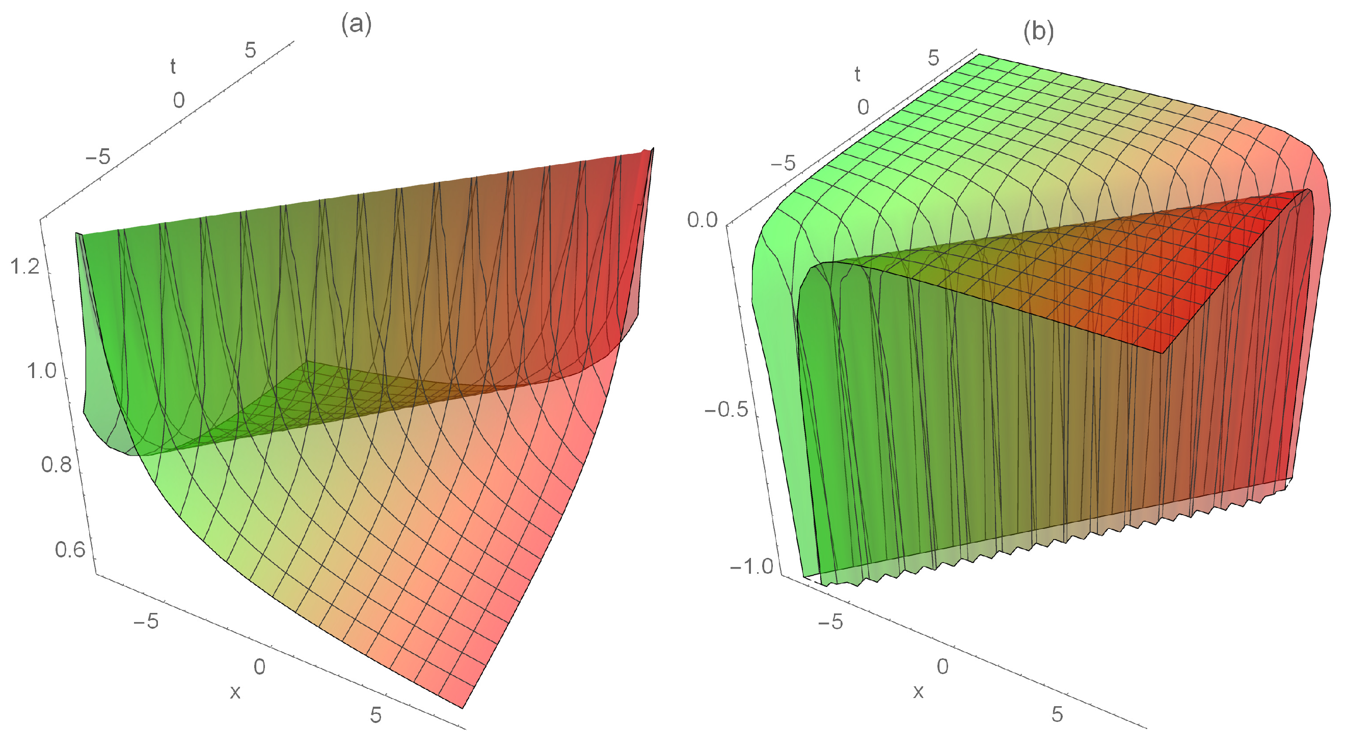
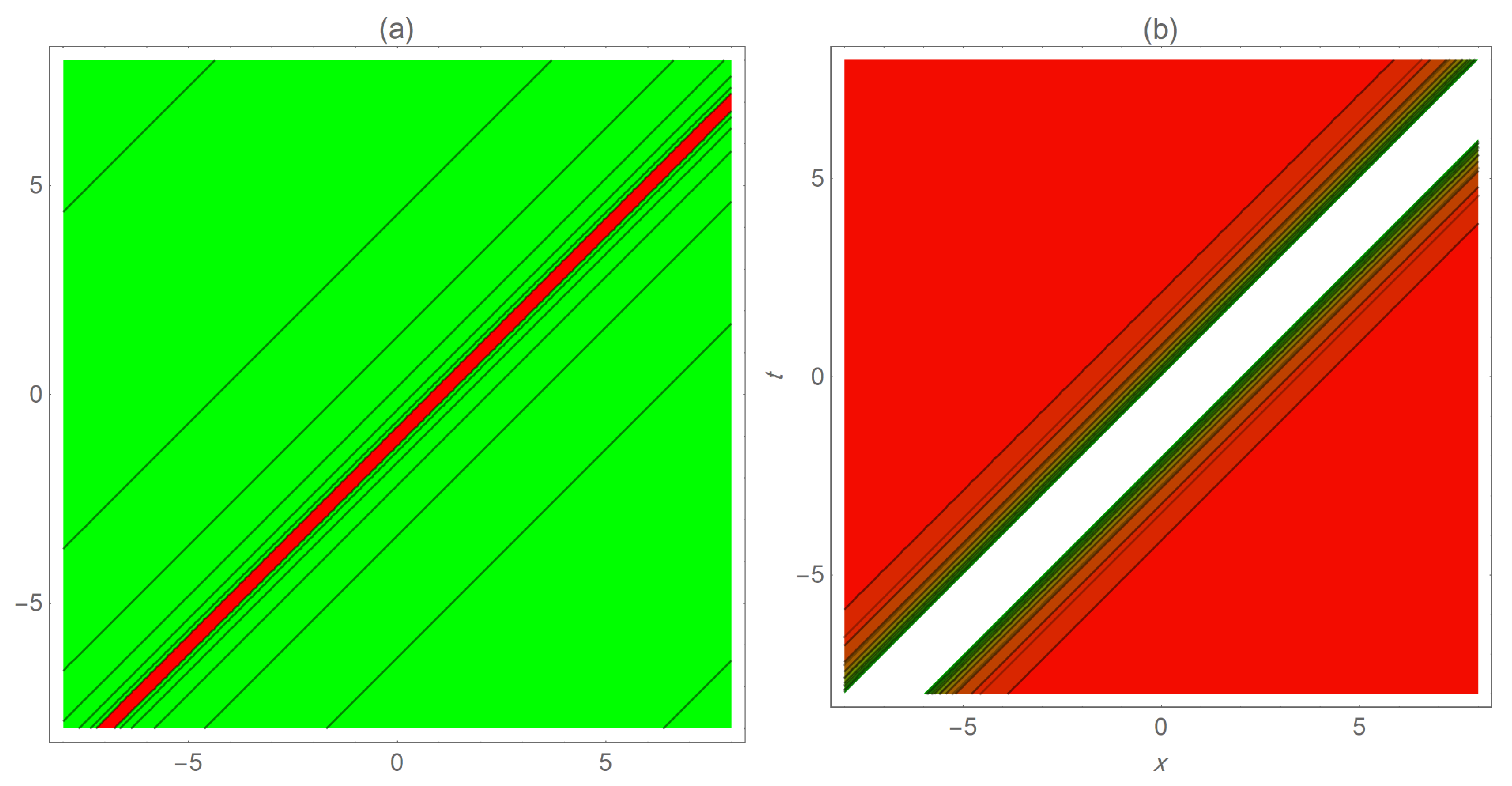
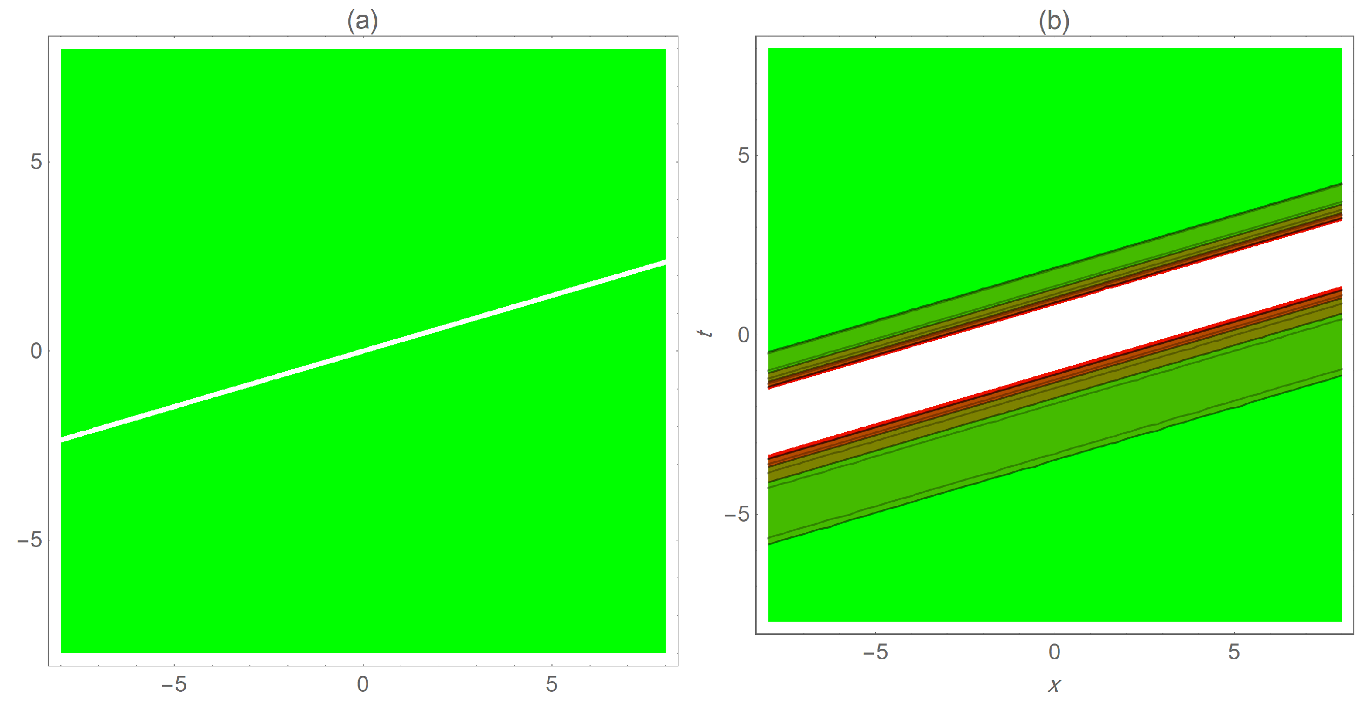
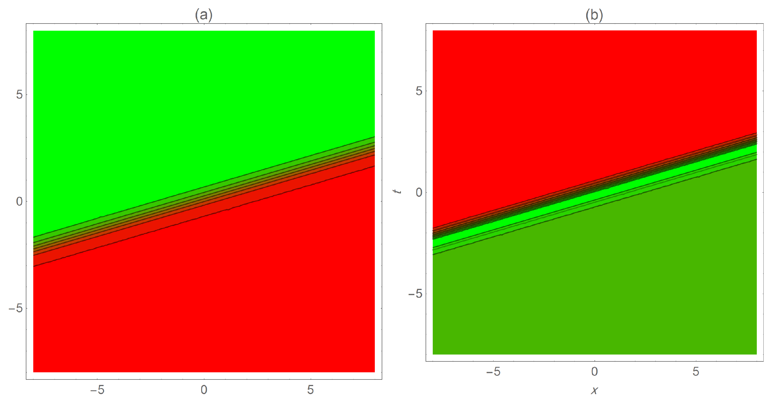
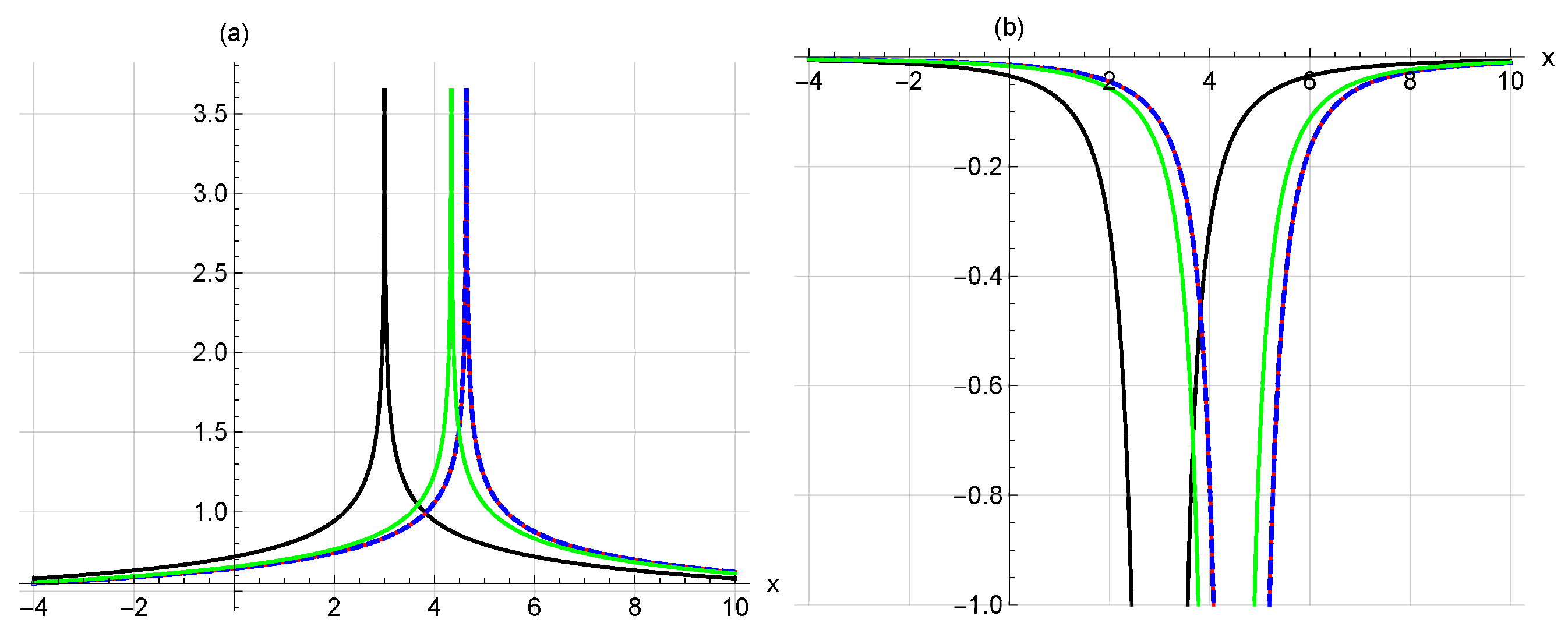
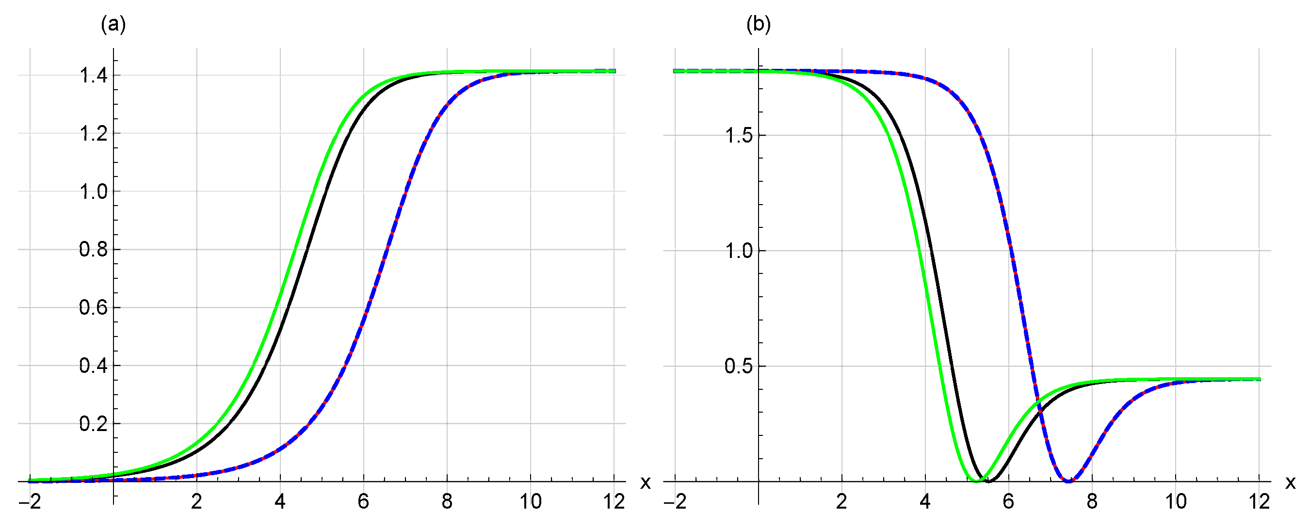
5. Graphical Representations

For comparison purposes, the basics of the comparative analysis, showing the dynamical behavior graphically of soliton solutions gives researchers vital indications of the wave motion of the particles under study. Here, several of the spatial solitons derived in the previous section are depicted in 3D. The corresponding contour plots are also listed to further clarify the wave motion.
Figure 1 shows the 3D bright and dark nematicons (Figure 1a and Figure 1b, respectively) of the reduced quadruple system in Equations (45) and (46). The parameters are fixed to be θ 0 = 1 ; n = 3 ; γ 1 = 1 ; γ 0 = 1 ; κ = 0.5 ; β = 1 ; α 1 = 1 ; α 2 = 1 ; α 4 = 1 ; α 5 = 1 ; and C 2 = 0.5 . The corresponding contour profiles are shown in Figure 2.
Notice that this generalized quadruple system can be solved using our expansion to obtain more closed-form nematic solutions. On the other hand, the generalized liquid crystal model, Equations (1)–(3), produces many sub-models with potential applications in optics theory.
In Figure 3 and Figure 4, the new dark nematicons and their contours for Equations (1)–(3) are depicted with θ 0 = 0 ; n = 1.5 ; κ = 1 ; α 1 = 1.7 ; α 2 = 0.9 ; α 3 = 1 ; α 4 = 1 ; α 5 = 1 ; A 1 = 1 ; and B 1 = 0.1 .
Figure 5 and Figure 6 show the new dark–kink spatial soliton solutions and their contours for our model with θ 0 = 0 ; n = 1 ; κ = 1 ; α 1 = 1.7 ; α 2 = 0.9 ; α 3 = 1 ; α 4 = 1 ; α 5 = 1 ; A 1 = 1 ; and B 1 = 1 .
The derived bright–dark nematicons in Equations (65) and (66) and corresponding contour plots are presented in Figure 7 and Figure 8, respectively. The parameters were θ 0 = 0 ;   n = 0.5 ; κ = 1 ; α 1 = 1.7 ; α 2 = 0.9 ; α 3 = 1 ; α 4 = 1 ; α 5 = 1 ; A 1 = 0.5 ; and B 1 = 0.5 .

6. Fractional Impacts

In the current section, the physical influences of the time–fractional modified Reimann–Liouville, β , and M-truncated derivatives on the solutions to the time–fractional version of the considered nematic liquid crystal model are shown and compared.
The mentioned derivatives are the most recently derived. In addition, the basic properties of the derivative, including the constant, linear, product, quotient, and chain rules, are satisfied.
In what follows, the basic concepts and properties of the used derivatives are listed.
Definition 1. 
(Jumarie’s modified Riemann–Liouville derivative (MRLD) [45] For μ 0 , 1 , the μth-order MRLD operator L is defined as
L t μ f t = 1 Γ μ d d t 0 t f τ f 0 t τ μ + 1 d τ , μ < 0 , 1 Γ 1 μ d d t 0 t f τ f 0 t τ μ d τ , 0 < μ < 1 , f μ k t k , 1 k μ < k + 1 ,
provided that f ( t ) is continuous on R + .
As mentioned before, the linearity, product, quotient, and chain rules are verified in the MRLD case. In addition, we have
L t μ t δ = Γ 1 + δ Γ 1 + δ μ t δ μ .
Definition 2. 
(Beta derivative (βD)) [46] For μ 0 , 1 , the μth-order β operator L is defined as
L t μ f t = lim ϵ 0 f t + ϵ t + 1 Γ μ 1 μ f t ϵ .
The β D satisfies the basic properties of the integer-order derivative. Moreover, the formula in Equation (68) and
L t μ t δ = t + 1 Γ μ 1 μ f t ,
provided that f ( t ) is differentiable, are verified.
Definition 3. 
(M-truncated derivative (MTD)) [47] For μ 0 , 1 , the μth-order MTD operator L is defined as
L M μ , ξ j f t = lim ϵ 0 f E ξ j ϵ t μ t f t ϵ , ξ > 0 ,
where
E ξ j ζ = i = 0 j ζ i Γ i ξ + 1 , ξ > 0 , ζ C ,
represents the single-parameter truncated Mittag–Leffler function.
The MTD satisfies the main derivative properties. In addition,
L M μ , ξ j f t = t 1 μ Γ ξ + 1 f t ,
provided that f ( t ) is differentiable, is verified.
The time–fractional version of the governed liquid crystal model in Equations (1)–(3) is written as
i L t μ q + α 1 2 q x 2 + α 2 p q = 0 ,
α 3 2 p x 2 + α 4 p + α 5 C 0 + C 1 q 2 n + C 2 q 4 n + C 3 q 6 n + C 4 q 8 n = 0 .
We consider the formal solutions in Equations (8) and (9) with traveling-wave transforms
η = β x ν t μ Γ μ + 1 ,
η = β x ν μ t + 1 Γ μ μ ,
and
β x ν Γ ( P + 1 ) t μ μ ,
regarding the MRL, β , and MT fractional derivatives, respectively. The rest of the solution steps are performed similar to that described in Section 3. The obtained nematicons will be as above with η replaced with its value in Equations (76)–(78), corresponding to each fractional derivative case.
In Figure 9, the 2D profiles of the nematicons in Figure 1 with the effects of various time–fractional operators, the MRLD, β D, and MTD, in comparison to the first derivative (black solid line) are shown.
Consequently, Figure 10, Figure 11 and Figure 12 present the time–fractional effects on the behaviors of the wave profile q ( x , t ) and tilt angle p ( x , t ) that are illustrated in Figure 3, Figure 5, and Figure 7, respectively.

7. Conclusions

This work aims to develop a new efficient way to obtain closed-form analytic solutions for nonlinear evolution problems governed by differential equations. The modification is based on merging two powerful schemes known as the modified simple equation method and the ansatz method. The suggested development shows the efficiency, applicability, and low complexity in comparison to other existing analyses.
The complex liquid crystal system with general quadruple nonlinearity forms the case study. This model is deduced by the balance between the linear deviation and nonlinear self-focusing of the input beam occurring for non-locality, a sequel resulting from the thermal response or redirection of the material to light.
Numerous spatial optical soliton (nematicon) solutions were derived for the considered model. Some of which are new. Bright, dark, and mixed peakon, cuspon, kink, and periodic-shaped nematicons were obtained and illustrated in 3D portraits.
The MSEM is based on the high skills of treating nonlinear ordinary systems. As shown in the first couple of cases in Equation (4), the obtained solutions appear in exponential form. Complexity is also faced while reformulating these solutions according to the choice of free parameters. The expanded version saves us the trouble of choosing, and direct formal hyperbolic and trigonometric solutions can be achieved.
The generalized Riccati equation mapping scheme was used to solve our model in [31]; it was shown that this method covers many other existing methods like the e ϕ η expansion G G expansion, t a n h c o t h , and t a n ( ϕ 2 ) methods. The expanded modified simple equation algorithm illustrates the possibility of deriving more spatial soliton and generic soliton solutions as shown in the cuspon, peakon, singular, and kink, both dark and bright, nematicons. Moreover, the expanded ansatz method [32] gives analytic solutions, which are considered to be special cases of those in the GREMM with a low cost. In summary, the examined method deduces more solutions with less complexity.
The obtained solutions can be expanded to obtain more soliton profiles by assuming the unknown function in the used ansatz. In our case, the secant, co-secant, and rival hyperbolic versions are ignored because of the similarity to the dynamic behaviors obtained by assuming the sine and cosine functions. Moreover, the tangent, cotangent, hyperbolic tangent, and hyperbolic cotangent ansatz are neglected since the resulting algebraic systems are not solvable, which addresses our previous claim.
On the other hand, the fractional effects, in different senses, are simulated. These effects are shown in comparison to the integer-order derivative in terms of the translation of the wave motion that depends on the chosen fraction and fixed time.
A motivating question remains: What about imposing ϕ in Equation (7) as an inverse trigonometric or hyperbolic function? The basic idea is to formulate ϕ , ϕ , … in terms of ϕ itself. In addition, is the obtained free-functional system solvable?

Author Contributions

Conceptualization, M.A.A.Z. and E.A.Z.-Z.; methodology, E.A.Z.-Z.; software, K.A.; validation, M.A.A.Z., K.A. and E.A.Z.-Z.; formal analysis, E.A.Z.-Z.; resources, E.A.Z.-Z. and M.A.A.Z.; data curation, E.A.Z.-Z.; writing—original draft preparation, E.A.Z.-Z.; writing—review and editing, M.A.A.Z. and K.A.; supervision, E.A.Z.-Z.; project administration, E.A.Z.-Z.; funding acquisition, K.A. All authors have read and agreed to the published version of the manuscript.

Funding

The authors extend their appreciation to the Deanship of Research and Graduate Studies at King Khalid University for funding this work through the Large Research Project under grant number RGP2/215/45.

Data Availability Statement

Dataset available on request from the authors.

Acknowledgments

The authors would like to express sincerely thanks to the referees for their useful comments and discussions.

Conflicts of Interest

The authors declare no conflicts of interest.

References

  1. Shi, S.; Han, D.; Cui, M. A multimodal hybrid parallel network intrusion detection model. Connect. Sci. 2023, 35, 2227780. [Google Scholar] [CrossRef]
  2. Zheng, Y.; Wang, Y.; Liu, J. Research on structure optimization and motion characteristics of wearable medical robotics based on Improved Particle Swarm Optimization Algorithm. Future Gener. Comput. Syst. 2022, 129, 187–198. [Google Scholar] [CrossRef]
  3. Faridi, W.A.; Bakar, M.A.; Riaz, M.B.; Myrzakulova, Z.; Myrzakulov, R.; Mostafa, M.A. Exploring the optical soliton solutions of Heisenberg ferromagnet-type of Akbota equation arising in surface geometry by explicit approach. Opt. Quantum Electron. 2024, 56, 1046. [Google Scholar] [CrossRef]
  4. Nadeem, M.; Iambor, L.F. Numerical Study of Time-Fractional Schrödinger Model in One-Dimensional Space Arising in Mathematical Physics. Fractal Fract. 2024, 8, 277. [Google Scholar] [CrossRef]
  5. Fei, R.; Guo, Y.; Li, J.; Hu, B.; Yang, L. An Improved BPNN Method Based on Probability Density for Indoor Location. IEICE Trans. Inf. Syst. 2023, 106, 773–785. [Google Scholar] [CrossRef]
  6. Az-Zo’bi, E. An approximate analytic solution for isentropic flow by an inviscid gas model. Arch. Mech. 2014, 66, 203–212. [Google Scholar]
  7. Sharma, N.; Alhawael, G.; Goswami, P.; Joshi, S. Variational iteration method for n-dimensional time-fractional Navier–Stokes equation. Appl. Math. Sci. Eng. 2024, 32, 2334387. [Google Scholar] [CrossRef]
  8. Moosavi Noori, S.R.; Taghizadeh, N. Study of Convergence of Reduced Differential Transform Method for Different Classes of Differential Equations. Int. J. Differ. Equ. 2021, 2021, 6696414. [Google Scholar] [CrossRef]
  9. Az-Zo’bi, E.A. Reliable analytic study for higher-dimensional telegraph equation. J. Math. Comput. Sci. 2018, 18, 423–429. [Google Scholar] [CrossRef]
  10. Kumar, S.; Malik, S.; Rezazadeh, H. The integrable Boussinesq equation and it’s breather, lump and soliton solutions. Nonlinear Dyn. 2022, 107, 2703–2716. [Google Scholar] [CrossRef]
  11. Ionescu, C.; Constantinescu, R. Optimal Choice of the Auxiliary Equation for Finding Symmetric Solutions of Reaction–Diffusion Equations. Symmetry 2024, 16, 335. [Google Scholar] [CrossRef]
  12. Rehman, H.U.; Seadawy, A.R.; Razzaq, S.; Rizvi, S.T. Optical fiber application of the Improved Generalized Riccati Equation Mapping method to the perturbed nonlinear Chen-Lee-Liu dynamical equation. Optik 2023, 290, 171309. [Google Scholar] [CrossRef]
  13. Fatema, K.; Islam, M.E.; Akhter, M.; Akbar, M.A.; Inc, M. Transcendental surface wave to the symmetric regularized long-wave equation. Phys. Lett. A 2022, 439, 128123. [Google Scholar] [CrossRef]
  14. Chen, H.; Zhu, Q.; Qi, J. Further results about the exact solutions of conformable space–time fractional Boussinesq equation (FBE) and breaking soliton (Calogero) equation. Results Phys. 2022, 37, 105428. [Google Scholar] [CrossRef]
  15. Liu, F.; Feng, Y. The modified generalized Kudryashov method for nonlinear space–time fractional partial differential equations of Schrödinger type. Results Phys. 2023, 53, 106914. [Google Scholar] [CrossRef]
  16. Alsharidi, A.K.; Bekir, A. Discovery of New Exact Wave Solutions to the M-Fractional Complex Three Coupled Maccari’s System by Sardar Sub-Equation Scheme. Symmetry 2023, 15, 1567. [Google Scholar] [CrossRef]
  17. Cao, Y.; Parvaneh, F.; Alamri, S.; Rajhi, A.A.; Anqi, A.E. Some exact wave solutions to a variety of the Schrödinger equation with two nonlinearity laws and conformable derivative. Results Phys. 2021, 31, 104929. [Google Scholar] [CrossRef]
  18. Bilal, M.; Ren, J. Dynamics of exact solitary wave solutions to the conformable time-space fractional model with reliable analytical approaches. Opt. Quant. Electron. 2022, 54, 40. [Google Scholar] [CrossRef]
  19. Assanto, G. Nematicons: Spatial Optical Solitons in Nematic Liquid Crystals; Wiley: Hoboken, NJ, USA, 2012. [Google Scholar]
  20. Peccianti, M.; Assanto, G. Nematicons. Phys. Rep. 2012, 516, 147–208. [Google Scholar] [CrossRef]
  21. Simoni, F. Nonlinear Optical Properties of Liquid Crystals; World Scientific Publishing: London, UK, 1997. [Google Scholar]
  22. Kumar, D.; Joardar, A.K.; Hoque, A.; Paul, G.C. Investigation of dynamics of nematicons in liquid crystals by extended sinh-Gordon equation expansion method. Opt. Quant. Electron. 2019, 51, 212. [Google Scholar] [CrossRef]
  23. Raza, N.; Afzal, U.; Butt, A.R.; Rezazadeh, H. Optical solitons in nematic liquid crystals with Kerr and parabolic law nonlinearities. Opt. Quant. Electron. 2019, 51, 107. [Google Scholar] [CrossRef]
  24. Ekici, M.; Mirzazadeh, M.; Sonmezoglu, A.; Ullah, M.Z.; Zhou, Q.; Moshokoa, S.P.; Biswas, A.; Belic, M. Nematicons in liquid crystals by extended trial equation method. J. Nonlinear. Opt. Phys. Mater. 2017, 26, 1750005. [Google Scholar] [CrossRef]
  25. Duran, S.; Karabulut, B. Nematicons in liquid crystals with Kerr Law by sub-equation method. Alex. Eng. J. 2022, 61, 1695–1700. [Google Scholar] [CrossRef]
  26. Ilhan, O.A.; Manafian, J.; Alizadeh, A.A.; Baskonus, H.M. New exact solutions for nematicons in liquid crystals by the tanϕ2- expansion method arising in fluid mechanics. Eur. Phys. J. Plus 2020, 135, 313. [Google Scholar] [CrossRef]
  27. Ismael, H.F.; Bulut, H.; Baskonus, H.M. W-shaped surfaces to the nematic liquid crystals with three nonlinearity laws. Soft Comput. 2021, 25, 4513–4524. [Google Scholar] [CrossRef]
  28. Kavitha, L.; Venkatesh, M.; Gopi, D. Shape changing nonlocal molecular deformations in a nematic liquid crystal system. J. Assoc. Arab. Univ. Basic Appl. Sci. 2015, 18, 29–45. [Google Scholar] [CrossRef]
  29. Savescu, M.; Johnson, S.; Sanchez, P.; Zhou, Q.; Mahmood, M.F.; Zerrad, E.; Biswas, A.; Belic, M. Nematicons in liquid crystals. J. Comput. Theor. Nanosci. 2015, 12, 4667–4673. [Google Scholar] [CrossRef]
  30. Marchant, T.R.; Smyth, N. Approximate techniques for dispersive shock waves in nonlinear media. J. Nonlinear Opt. Phys. Mater. 2012, 21, 1250035. [Google Scholar] [CrossRef]
  31. Altawallbeh, Z.; Az-Zo’bi, E.; Alleddawi, A.O.; Şenol, M.; Akinyemi, L. Novel liquid crystals model and its nematicons. Opt. Quant. Electron. 2022, 54, 861. [Google Scholar] [CrossRef]
  32. Az-Zo’bi, E.A.; Afef, K.; Ur Rahman, R.; Akinyemi, L.; Bekir, A.; Ahmad, H.; Tashtoush, M.A.; Mahariq, I. Novel topological, non-topological, and more solitons of the generalized cubic p-system describing isothermal flux. Opt. Quant. Electron. 2024, 56, 84. [Google Scholar] [CrossRef]
  33. Jawad, A.J.M.; Petković, M.D.; Biswas, A. Modified simple equation method for nonlinear evolution equations. Appl. Math. Comput. 2010, 217, 869–877. [Google Scholar]
  34. Zayed, E.M.E.; Ibrahim, S.A.H. Exact solutions of nonlinear evolution equations in mathematical physics using the modified simple equation method. Chin. Phys. Lett. 2012, 29, 060201. [Google Scholar] [CrossRef]
  35. Khan, K.; Akbar, M.A.; Ali, N.H. The Modified Simple Equation Method for Exact and Solitary Wave Solutions of Nonlinear Evolution Equation: The GZK-BBM Equation and Right-Handed Noncommutative Burgers Equations. Int. Sch. Res. Not. 2013, 2013, 146704. [Google Scholar] [CrossRef]
  36. Az-Zo’bi, E.A. New kink solutions for the van der Waals p-system. Math. Methods Appl. Sci. 2019, 42, 6216–6226. [Google Scholar] [CrossRef]
  37. Al-Amr, M.O.; El-Ganaini, S. New exact traveling wave solutions of the (4+1)-dimensional Fokas equation. Comput. Math. Appl. 2017, 74, 1274–1287. [Google Scholar] [CrossRef]
  38. Zhao, Y.-M.; He, Y.-H.; Long, Y. The simplest equation method and its application for solving the nonlinear NLSE, KGZ, GDS, DS, and GZ equations. J. Appl. Math. 2013, 7, 960798. [Google Scholar] [CrossRef]
  39. Az-Zo’bi, E.A.; AlZoubi, W.A.; Akinyemi, L.; Şenol, M.; Alsaraireh, I.W.; Mamat, M. Abundant closed-form solitons for time-fractional integro–differential equation in fluid dynamics. Opt. Quant. Electron. 2021, 53, 132. [Google Scholar] [CrossRef]
  40. Al-Amr, M.O.; Rezazadeh, H.; Ali, K.K.; Korkmazki, A. N1-soliton solution for Schrödinger equation with competing weakly nonlocal and parabolic law nonlinearities. Commun. Theor. Phys. 2020, 72, 065503. [Google Scholar] [CrossRef]
  41. Rasheed, N.M.; Al-Amr, M.O.; Az-Zo’bi, E.A.; Tashtoush, M.A.; Akinyemi, L. Stable Optical Solitons for the Higher-Order Non-Kerr NLSE via the Modified Simple Equation Method. Mathematics 2021, 9, 1986. [Google Scholar] [CrossRef]
  42. Bakıcıerler, G.; Alfaqeih, S.; Mısırlı, E. Application of the modified simple equation method for solving two nonlinear time-fractional long water wave equations. Revista Mexicana de Fısica 2021, 67, 060701. [Google Scholar]
  43. Bakıcıerler, G.; Mısırlı, E. Some New Traveling Wave Solutions of Nonlinear Fluid Models via the MSE Method. Fundam. J. Math. Appl. 2021, 4, 187–194. [Google Scholar]
  44. Az-Zo’bi, E.A. Peakon and solitary wave solutions for the modified Fornberg-Whitham equation using simplest equation method. Int. J. Math. Comput. Sci. 2019, 14, 635–645. [Google Scholar]
  45. Jumarie, G. Modified Riemann-Liouville derivative and fractional Taylor series of nondifferentiable functions further results. Comput. Math. Appl. 2006, 51, 1367–1376. [Google Scholar] [CrossRef]
  46. Atangana, A.; Baleanu, D.; Alsaedi, A. Analysis of time-fractional hunter-saxton equation: A model of neumatic liquid crystal. Open Phys. 2016, 14, 145–149. [Google Scholar] [CrossRef]
  47. da Sousa, J.V.C.; de Oliveira, E.C. A new truncated M-fractional derivative type unifying some fractional derivative types with classical properties. arXiv 2017, arXiv:1704.08187. [Google Scholar]
Figure 1. Three-dimensional (a) peakon-shaped and (b) cuspon-shaped (singular kink) nematicons of the wave profile and tilt angle in Equations (47) and (48).
Symmetry 16 00778 g001
Figure 2. Contour plots of the (a) peakon-shaped and (b) cuspon-shaped nematicons in Figure 1.
Symmetry 16 00778 g002
Figure 3. Three-dimensional singular kink nematicons of the (a) wave profile and (b) tilt angle in Equations (50) and (51).
Symmetry 16 00778 g003
Figure 4. Contour plots of the (a) wave profile and (b) tilt angle in Figure 3.
Symmetry 16 00778 g004
Figure 5. Three-dimensional kink nematicons of the (a) wave profile and (b) tilt angle in Equations (55) and (56).
Symmetry 16 00778 g005
Figure 6. Contour plots of the (a) wave profile and (b) tilt angle in Figure 5.
Symmetry 16 00778 g006
Figure 7. Three-dimensional singular-periodic nematicons of the (a) wave profile and (b) tilt angle in Equations (65) and (66).
Symmetry 16 00778 g007
Figure 8. Contour plots of the (a) wave profile and (b) tilt angle in Figure 7.
Symmetry 16 00778 g008
Figure 9. 0.3 th-order time–fractional using MRLD (red solid), β D (blue dashed), and MTD (green line) of the (a) peakon-shaped wave profile and (b) cuspon-shaped tilt angle in Equations (47) and (48) at t = 1 .
Symmetry 16 00778 g009
Figure 10. 0.7 th-order time–fractional using MRLD (red solid), β D (blue dashed), and MTD (green line) of the singular kink (a) wave profile and (b) tilt angle in Equations (50) and (51) at t = 1 .
Symmetry 16 00778 g010
Figure 11. 0.5 th-order time–fractional using MRLD (red solid), β D (blue dashed), and MTD (green line) of the kink (a) wave profile and (b) tilt angle in Equations (55) and (56) at t = 0.5 .
Symmetry 16 00778 g011
Figure 12. 0.5 th-order time–fractional using MRLD (red solid), β D (blue dashed), and MTD (green line) of the periodic (a) wave profile and (b) tilt angle in Equations (65) and (66) at t = 0.5 .
Symmetry 16 00778 g012
Disclaimer/Publisher’s Note: The statements, opinions and data contained in all publications are solely those of the individual author(s) and contributor(s) and not of MDPI and/or the editor(s). MDPI and/or the editor(s) disclaim responsibility for any injury to people or property resulting from any ideas, methods, instructions or products referred to in the content.

