Abstract
With the rapid development of new-generation artificial intelligence and Internet of Things technology, mobile robot technology has been widely used in various fields. Among them, the autonomous path-planning technology of mobile robots is one of the cores for realizing their autonomous driving and obstacle avoidance. This study conducts an in-depth discussion on the real-time and dynamic obstacle avoidance capabilities of mobile robot path planning. First, we proposed a preprocessing method for obstacles in the grid map, focusing on the closed processing of the internal space of concave obstacles to ensure the feasibility of the path while effectively reducing the number of grid nodes searched by the A* algorithm, thereby improving path search efficiency. Secondly, in order to achieve static global path planning, this study adopts the A algorithm. However, in practice, algorithm A has problems such as a large number of node traversals, low search efficiency, redundant path nodes, and uneven turning angles. To solve these problems, we optimized the A* algorithm, focusing on optimizing the heuristic function and weight coefficient to reduce the number of node traversals and improve search efficiency. In addition, we use the Bezier curve method to smooth the path and remove redundant nodes, thereby reducing the turning angle. Then, in order to achieve dynamic local path planning, this study adopts the artificial potential field method. However, the artificial potential field method has the problems of unreachable target points and local minima. In order to solve these problems, we optimized the repulsion field so that the target point is at the lowest point of the global energy of the gravitational field and the repulsive field and eliminated the local optimal point. Finally, for the path-planning problem of mobile robots in dynamic environments, this study proposes a hybrid path-planning method based on a combination of the improved A* algorithm and the artificial potential field method. In this study, we not only focus on the efficiency of mobile robot path planning and real-time dynamic obstacle avoidance capabilities but also pay special attention to the symmetry of the final path. By introducing symmetry, we can more intuitively judge whether the path is close to the optimal state. Symmetry is an important criterion for us to evaluate the performance of the final path.
1. Introduction
In recent years, with the continuous advancement of technology, the field of mobile robotics has experienced rapid development. Mobile robots have not only significantly improved work efficiency and ensured production quality and precision but also have the capability to substitute humans in handling tasks in dangerous situations, bringing many conveniences to human production and life [1]. Therefore, research in the field of mobile robotics has become increasingly important, attracting widespread attention from researchers [2].
In the field of mobile robotics, path planning is one of the important research directions, facing the challenge of achieving collision-free movement of robots in complex environments [3]. The goal of path planning is to find the optimal path from the starting point to the destination based on one or more performance indicators. Depending on the degree of understanding of the surrounding environment, path planning can be divided into local path planning based on sensor information and global path planning based on known information [4]. Local path planning focuses on utilizing real-time environmental information obtained from sensors to achieve effective obstacle avoidance for robots, with common algorithms including the artificial potential field method, polynomial curve method, and dynamic window method. On the other hand, global path planning is based on known maps or environmental information to find the optimal path through global search and planning algorithms [5]. Global path planning algorithms are typically categorized into graph-based algorithms such as Dijkstra’s algorithm and A* algorithm and sampling-based search algorithms such as random path graph method, RRT algorithm, genetic algorithm, and ant colony algorithm [6,7].
A single global path planning algorithm can find the optimal trajectory but cannot perform dynamic obstacle avoidance. On the contrary, a local path planning algorithm can perform dynamic obstacle avoidance but cannot guarantee the performance of the trajectory. A hybrid algorithm that combines the two can combine the advantages of both, finding the global optimal path and performing dynamic obstacle avoidance, and can solve the problem of mobile robot navigation in complex environments. This paper innovatively proposes a fusion algorithm that combines the A* algorithm and the artificial potential field method, aiming to improve the autonomous navigation and obstacle avoidance capabilities of mobile robots in complex environments; compared with other algorithms, this fusion algorithm is lightweight and efficient. The A* algorithm combines the characteristics of depth-first search (DFS) and breadth-first search (BFS) to enhance search efficiency while finding the optimal path. However, this algorithm has significant drawbacks, including a large number of overall node traversals, low search efficiency, redundant path nodes, and non-smooth path turning angles. To address these shortcomings, scholars, both domestically and internationally, have conducted extensive research and exploration aimed at improving the performance of the A* algorithm [8]. The main directions of improvement include the following:
- (1)
- Improving the heuristic function: The heuristic function plays a significant role in determining the direction of search expansion. By enhancing the heuristic function, the accuracy and efficiency of the search can be improved;
- (2)
- Enhancing the weighting coefficients of the estimation function: The weighting coefficients determine whether the search process tends more towards breadth or depth. Optimizing these coefficients can better guide the search direction;
- (3)
- Optimizing the search domain: Reducing the search domain in special cases can significantly decrease the number of search nodes, thereby enhancing search efficiency;
- (4)
- Path curve optimization: Smoothing the path to make it more suitable for robot movement, reducing the problems of redundant path nodes and non-smooth turning angles;
- (5)
- Improving search strategies: Introducing strategies such as bidirectional search and jump point search (JPS) can significantly accelerate search efficiency.
These improvement measures are expected to further enhance the performance of the A* algorithm, making it more effective and reliable in practical applications.
The artificial potential field method is a widely utilized algorithm in path planning, characterized by its intuitive concept, ease of understanding, and implementation, as well as its excellent real-time performance, allowing timely responses to environmental changes, making it suitable for dynamic environment path planning. This method simulates obstacle repulsion forces using potential fields to effectively achieve obstacle avoidance and can be flexibly integrated and improved with other path planning algorithms or sensor information. However, the original artificial potential field method may fall into local optima, making it difficult to find the global optimal path. During obstacle avoidance, issues such as the robot being unable to reach the target point may arise due to the existence of repulsive forces [9,10,11]. This paper aims to address these issues through the following improvements:
- (1)
- Improving the repulsive force function to ensure that the target point lies at the global potential energy minimum of the attractive and repulsive fields;
- (2)
- Introducing global planning by combining with global path planning algorithms such as the A* algorithm to avoid falling into local optima;
- (3)
- Dynamically adjusting parameters based on real-time environmental information to adapt the potential field function and parameters to different scenarios;
- (4)
- Smoothing the generated paths to enhance robot mobility efficiency.
Section 1 of this paper mainly introduces the development of mobile robots, focusing on trajectory planning and obstacle avoidance problems in the navigation process. This paper is committed to proposing a hybrid path planning method based on the combination of improved A* algorithm and artificial potential field method to solve the navigation of mobile robots in complex environments, so the defects of A* algorithm and artificial potential field method are analyzed in the first chapter.
Section 2 of this paper mainly introduces and improves the methods used, including the map construction algorithm, A* algorithm, artificial potential field method, Bessel optimization algorithm, and fusion algorithm. The process of integrating various methods is described at the beginning of the second chapter.
Section 3 mainly conducts experiments and analysis, respectively testing the efficiency of the map preprocessing optimization algorithm, the difference in results under different parameters of the A* algorithm, and the comparison of the results of the hybrid algorithm and other algorithms.
Section 4 discusses the design of this paper and summarizes the innovative contributions and shortcomings of this paper.
2. Materials and Methods
The purpose of this chapter is to propose a dynamic path-planning method for mobile robots that comprehensively use the improved A* algorithm and artificial potential field method. To this end, this chapter is divided into four main parts to systematically explore the implementation of this method.
First of all, we will focus on the construction of global maps and map preprocessing optimization algorithms. This step is essential to ensure the accuracy and efficiency of subsequent path planning. Therefore, we will conduct an in-depth discussion of the map construction process and propose a series of optimization algorithms to improve the quality and processing efficiency of map data.
Secondly, we will explain in detail the application method of the improved A algorithm in global static path planning. Through the optimization and improvement of the A algorithm, we aim to overcome its high computational complexity and low search efficiency on large-scale maps so as to achieve faster and more accurate path planning.
Next, we will introduce a local dynamic path planning method based on an improved artificial potential field. As a commonly used dynamic path planning technique, the artificial potential field method can effectively cope with dynamic obstacles and changes in the environment. We will propose an optimized artificial potential field method to improve the accuracy and robustness of path planning.
Finally, we will discuss the trajectory curve optimization method based on the n-order Bezier curve. This method aims to further optimize the robot path to make it smoother and more efficient. At the same time, we will design a fusion algorithm that organically combines the improved A* algorithm, artificial potential field method, and Bezier curve optimization method to achieve a more comprehensive and effective dynamic path planning scheme. Through the comprehensive analysis and evaluation of these methods, we will provide a more in-depth and comprehensive solution to the path-planning problem of mobile robots.
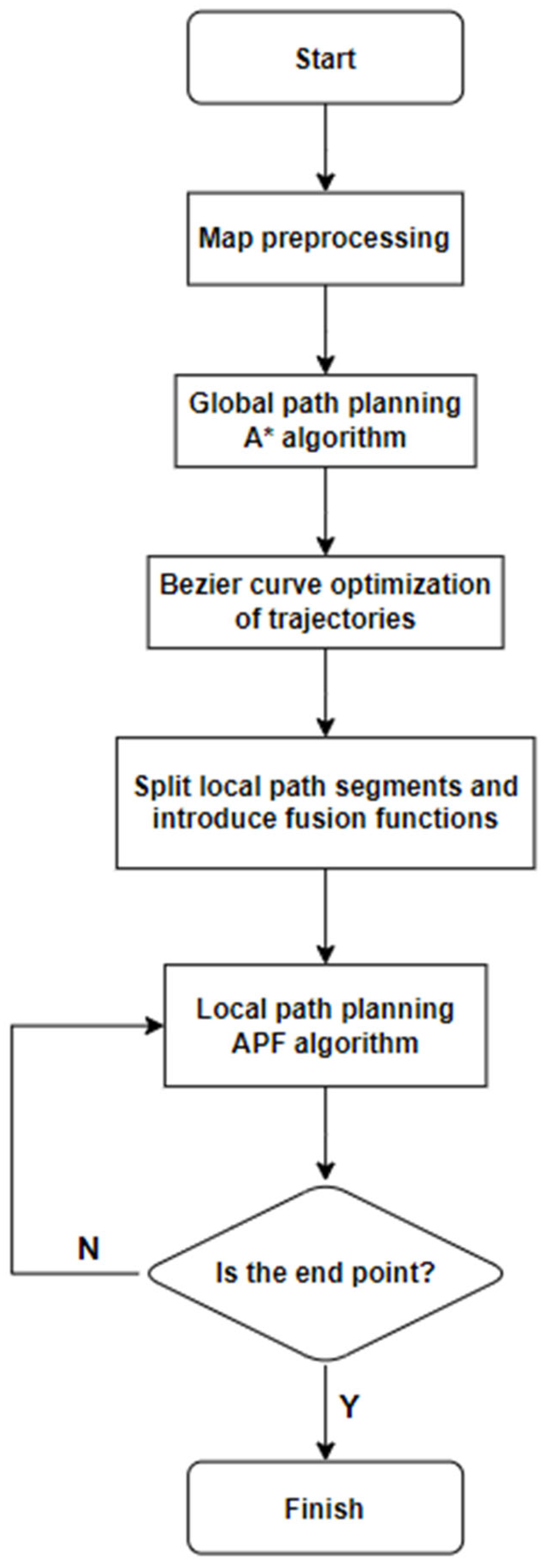
Figure 1 shows the overall process of the program after integrating various algorithms.
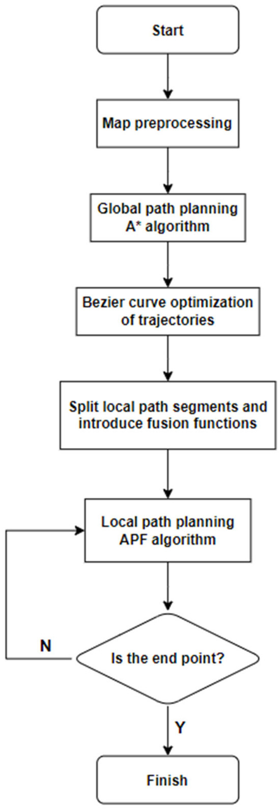
Figure 1.
Fusion algorithm flow chart.
Figure 1 shows the overall flow of the program after the fusion of various algorithms.
The program starts with preprocessing and optimizing the map to improve the search efficiency, then uses the A* algorithm for global path planning to obtain the optimal reference trajectory, performs Bezier optimization on the trajectory to meet the motion constraints, and finally segments the trajectory and introduces the fusion function to use the APF algorithm for local path planning until the end point is reached.
- Map creation and optimization;
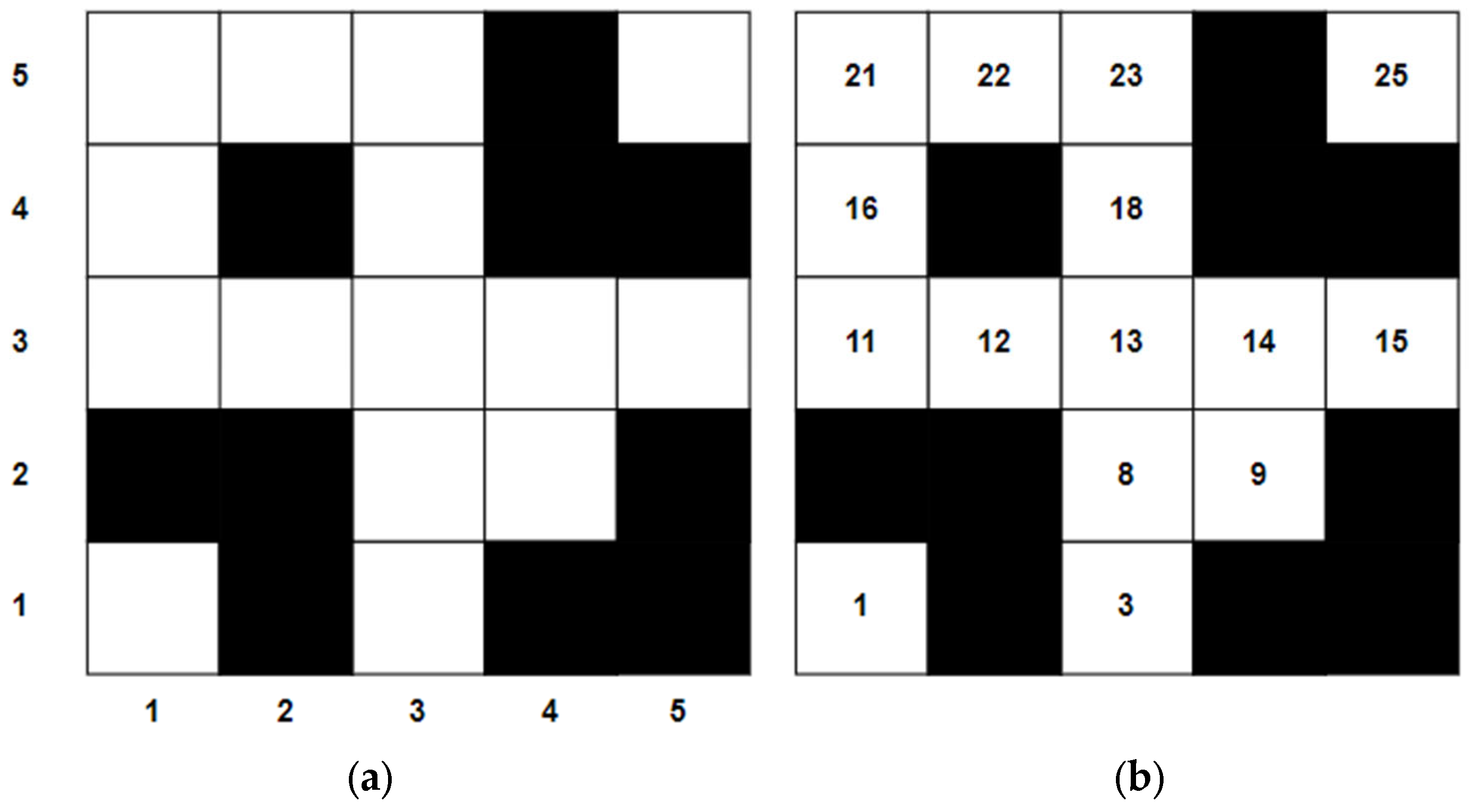
At present, the grid method mainly adopts two commonly used marking methods, the ordered numbering method and the coordinate method, as shown in Figure 2. Figure 2a shows a grid map marking method using cartesian coordinates. Cartesian coordinates place the origin of the cartesian coordinate system in the appropriate position in the grid map, usually in the lower-left corner of the grid map. Then, the X and Y axes are established in the horizontal and vertical directions of the map, and the unit length of the axis is generally equal to the side length of the grid. Therefore, the position of the grid can be represented by two-dimensional coordinates. In contrast, the serial number method is to mark the grid map sequentially according to a certain rule, and there is only one mark for each grid. Usually, the first grid in the lower left corner of the grid map is marked as the serial number 1, as shown in Figure 2b.
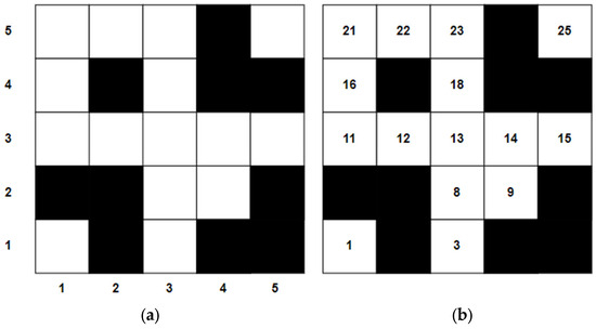
Figure 2.
Common layout methods for grid maps. (a) Cartesian coordinate mark; (b) position mark.
In the code writing of path planning algorithms, grid maps marked by cartesian coordinates are more commonly used. This is because the cartesian coordinate method can clearly display the relative positional relationship between obstacles and obstacles, and it is easy to analyze the influence of the distribution of different obstacles on path search. In contrast, grid maps marked by the serial number method are not easy to perform such analysis. After completing the grid marking, the algorithm can perform a path search based on the attributes of the mark and the grid. The principle of the grid method is simple and easy to implement, so in this study, the grid method based on cartesian coordinate marking is used to complete the map preprocessing algorithm.
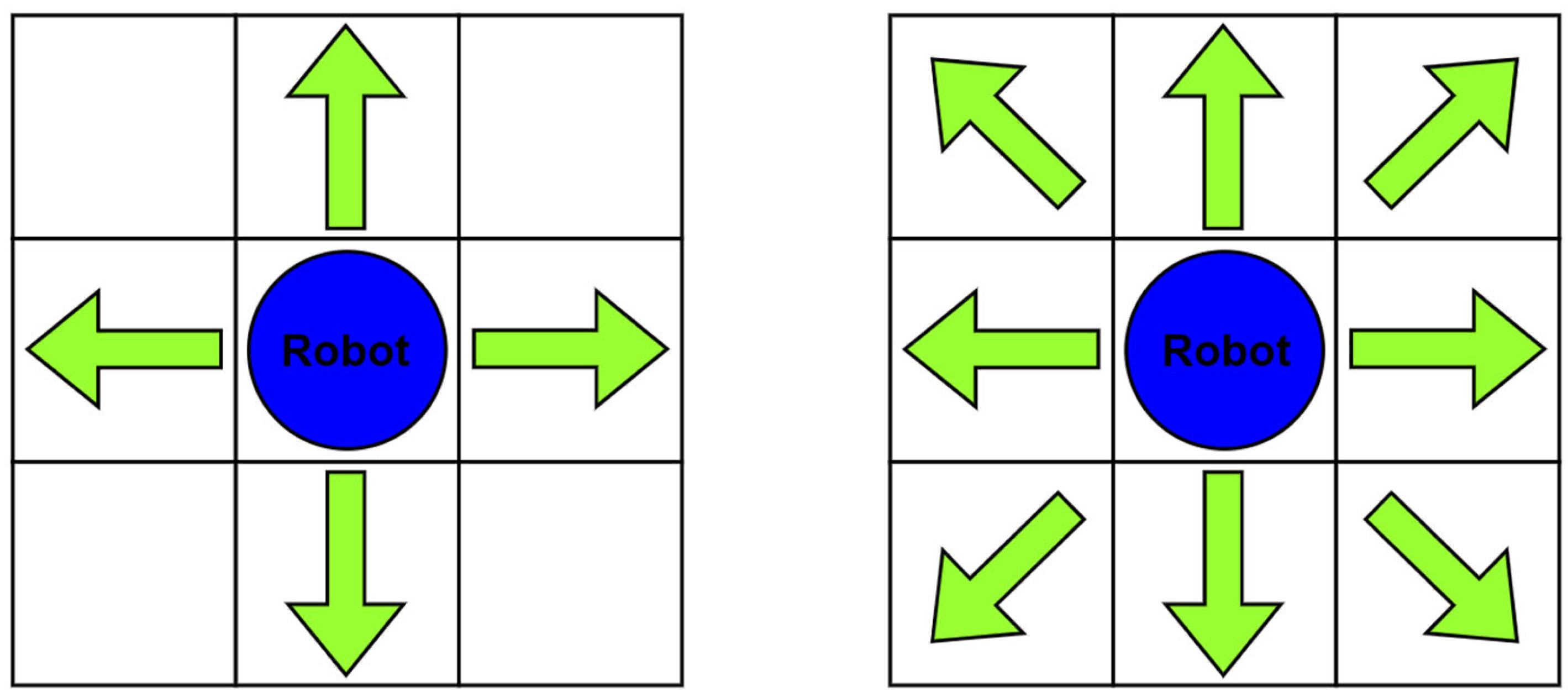
In the grid map, the grid is mainly divided into two categories: free grid and obstacle grid. Mobile robots usually use two methods: four-neighborhood search and eight-neighborhood search in grid maps. From the perspective of the calculation time of path search, the calculation amount of a four-neighborhood search is only half that of an eight-neighborhood search, so the time required for path search is shorter. However, from the perspective of the feasibility and length of the path, the path searched by the four neighbors has more turning corners, and each turning point is a ninety-degree right angle, which is not friendly to the actual movement of the mobile robot. In contrast, the path of the eight-neighborhood search can be planned through the diagonal of the grid, and the path length is better than that of the four-neighborhood search, as shown in Figure 3 Therefore, in this study, the grid maps all use the method of the eight-neighborhood search.
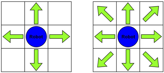
Figure 3.
Four-field search and eight-field search.
The problem of solving the optimal path by the grid method can be expressed in a mathematical model. In this study, the eight-neighborhood search method is used. The constructed grid map has a total of rows and columns. The grid coordinates of the starting position of the mobile robot are , and the grid coordinates of the k-step calculation are denoted as , and the grid coordinates of the target location are . The length of the path traveled by the mobile robot can be calculated by the number of grids traveled. E represents the collection of grids in the grid map.
indicates whether there are obstacles to the grid with coordinates :
represents the set of valid grids that can be selected when the mobile robot is located at the grid in the next step:
means that the mobile robot starts from the grid with coordinates and can select the grid after n steps:
P represents the collection of all free rasters in the entire grid map:
L represents the set of all feasible paths connecting the starting point and the target point. When solving the path planning problem, the path length J needs to reach the minimum value:
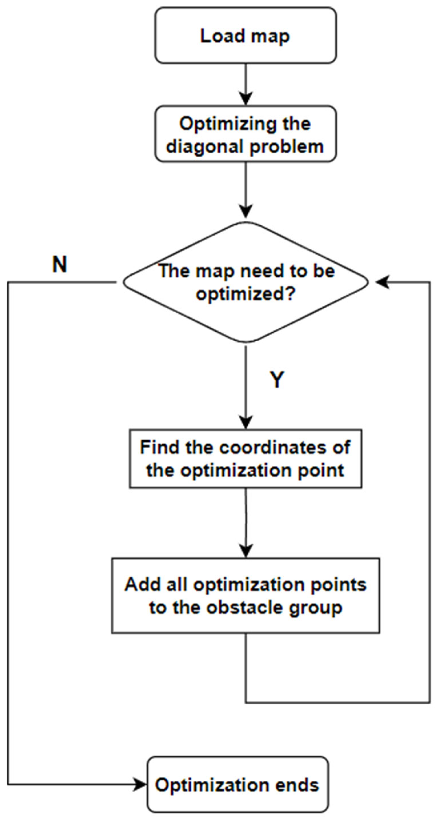
Equation (3) means that every time the mobile robot moves, it can select the grid in eight adjacent directions as the next forward grid; Equation (4) means that the grid selected by the mobile robot each time must be a free grid; Equation (5) means that the feasible solution to the pathfinding problem must be from the starting grid and finally reach the target grid; Equation (6) guarantees that the searched path is the shortest in length, and at the same time, the requirements of these formulas can find a collision-free shortest path in the grid map. In actual path planning, the disordered distribution of obstacles may cause mobile robots to perform unnecessary node searches inside certain concave obstacles, thereby increasing the search time and reducing the efficiency of path planning. Due to the influence of the mobile robot’s own volume, the search path may be invalid and may have other problems. In order to solve these problems, this research proposes a grid map preprocessing algorithm based on the selection of coordinate maps, which aims to complement the search algorithm to improve the efficiency of path search. The improvement of the algorithm is mainly reflected in the following aspects. The map optimization algorithm process is shown in Figure 4.
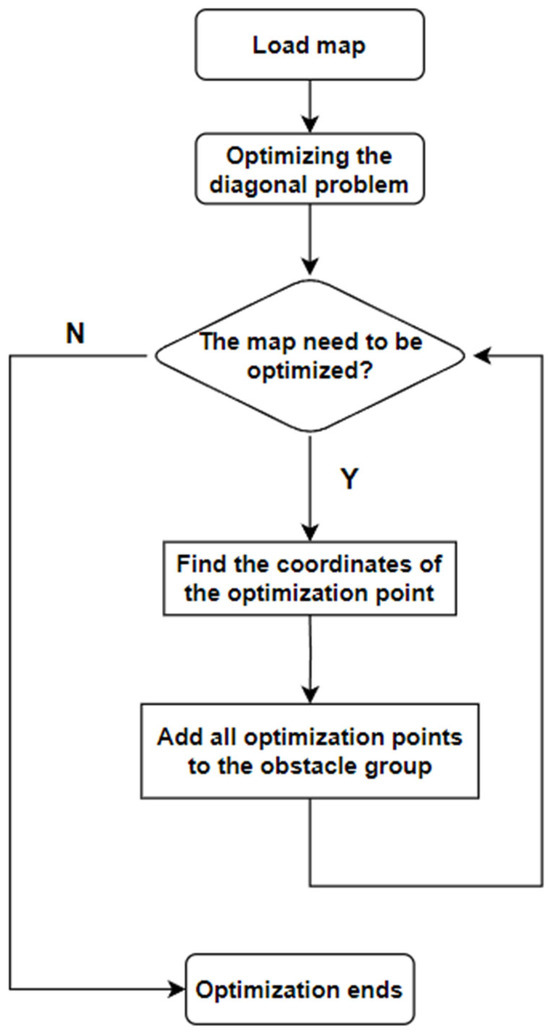
Figure 4.
Execution sequence flow of map preprocessing algorithm.
First of all, the problem that the robot cannot reach when crossing the diagonal is solved, and the availability of the planned path is ensured. Secondly, it can close concave obstacles and reduce the search algorithm’s search for invalid grid nodes or trap areas during path search, thereby improving the efficiency of path search.
- The A* algorithm and its optimization;
The A* algorithm draws upon the principles of the Dijkstra algorithm and the Best-First Search algorithm, employing heuristic search to explore from the starting point to the target point within a map environment. Its heuristic search method comprises the edge cost and Euclidean distance. The core idea of this algorithm is to plan a path from the starting point to the target point with the minimum movement cost in the map environment [12]. The evaluation function for the movement cost is defined as follows:
In the formula, is the current search node of the A* algorithm, f(n) is the total generation value of the current node, g(n) is the cost value from the starting point to the current node n in the map, h(n) is the current node and the target Estimated cost between points.
For the A* algorithm, the quality of the evaluation function will directly affect the efficiency of the path search. If h(x) is 0, then only g(x) is contributing to the path search. At this time, the A* and Dijkstra algorithm path-finding effect is the same. The advantage is that the shortest path can be found, but the disadvantage is that the calculation time is long. At this time, the focus is on breadth priority. If h(x) is always smaller than g(x) when the A* algorithm searches for a path, the A* algorithm is guaranteed to find the shortest path, and the smaller the value of h(x), the grid node searched by the A* algorithm will be, the more, the longer the calculation time will be. On the contrary, the larger the value of h(x), the more “greedy” the search will be, and the shorter the time will be. At this time, focus on depth priority [13,14].
This article introduces a weight coefficient here, to balance the breadth and depth of the search (n):
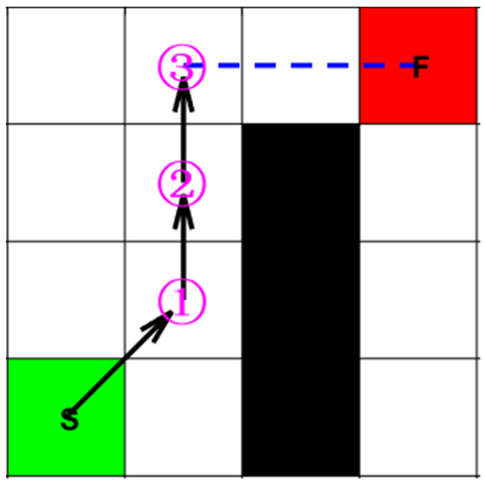
The cost value g(n) of the A* algorithm from the starting point in the map to the current node n is quantified by the real moving distance from the starting point to the current node n. During the search process, the cost value g(n) is between the current node n and the cost value g(n). The relationship is shown in Figure 5.

Figure 5.
Relationship diagram between node n and g(n).
In the figure, “S” represents the starting point, “F” represents the target point, the black region indicates obstacles in the map environment, “2” represents the current node n, “1” represents the parent node n − 1, and “3” represents the child node n + 1. The actual distance from the starting point “S” to node “1” is denoted as S(1), and the actual distance from node “1” to node “2” is denoted as S(2), and so forth. The actual distance from the current node “n” to the parent node “n − 1” is denoted as S(n). “g(n)” represents the sum of actual distances from the starting point to the current node “n”. Thus, the mathematical expression for the actual cost function “g(n)” is given by Equation (9).
In Figure 5, the distance between the current node 3 and the target point F is the estimated cost heuristic function . Commonly used calculation methods for the estimated cost heuristic function include Euclidean distance and Manhattan distance. There are three types of distance, including Chebyshev distance [15]. This article uses the Euclidean distance with the highest calculation accuracy. Assume that the coordinates of the current node in the map environment are and the coordinates of the target point are .
The Grid distance is shown in Equation (10):
The Manhattan distance is shown in Equation (11):
The Chebyshev distance is shown in Equation (12):
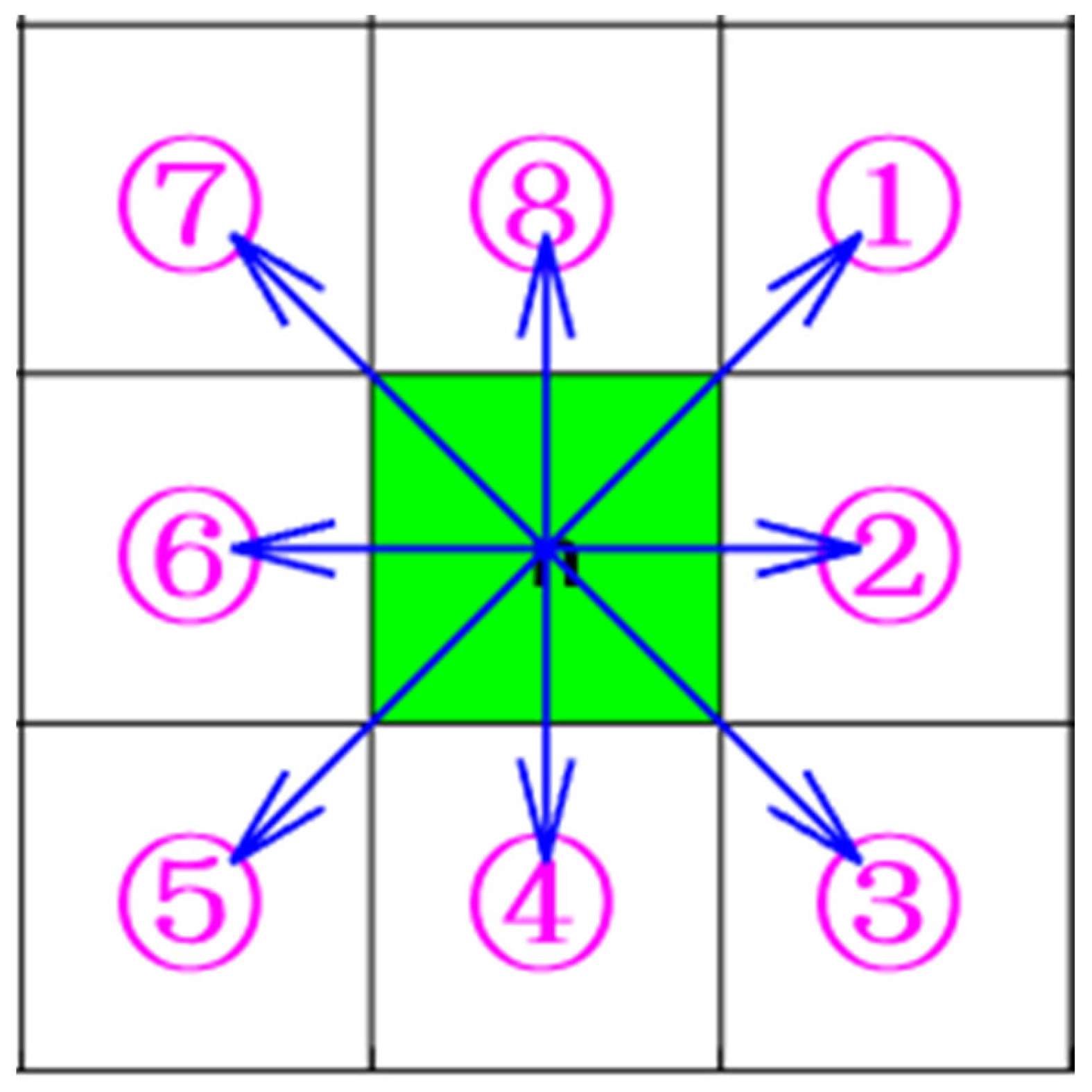
The A* algorithm simultaneously calculates the values of h(n) and g(n) during the pathfinding process and finds the optimal path in the direction approaching the target point while ensuring search efficiency. During the search process, the A* algorithm will traverse the eight adjacent nodes of each node in the search direction, that is, the eight-neighborhood search. Figure 6 is a schematic diagram of the eight-neighborhood search of the A* algorithm.
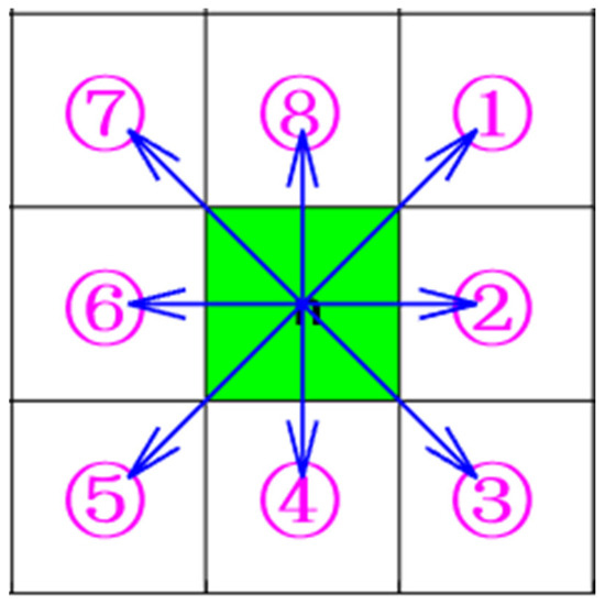
Figure 6.
A* algorithm 8 domain search.
The A* algorithm utilizes an eight-neighborhood search process, where the eight grids surrounding each grid in the graph represent the neighborhood to be searched by the A* algorithm at that node. During the execution of the A* algorithm, these grids are placed in the OpenList, and after traversal, the grid with the minimum cost is selected and placed in the ClosedList as the next node. This process continues until the algorithm reaches the target point, as illustrated in the graph: S → 1 → 2 → 3 → F.
The A* algorithm systematically searches grid nodes using an evaluation function, which assigns a heuristic value to each node along the path, effectively measuring the quality of each node on the optimal path. Consequently, the A* algorithm can find the optimal path. However, the algorithm also has several drawbacks. Firstly, it often finds a local optimal path rather than a global optimal path. This is because the A* algorithm evaluates the cost of only a subset of nodes on the grid map rather than searching all grid nodes. Thus, in complex map environments, the A* algorithm may fail to identify the global optimal path. Secondly, although searching in an eight-neighborhood provides more possibilities for path feasibility, exploring each step involves searching eight neighboring grids, and even in the absence of obstacles, grid nodes are repeatedly searched, leading to longer computation times and reduced efficiency. Lastly, the paths generated by the A* algorithm on grid maps typically contain many line segments, which are not conducive to the actual movement of mobile robots [16,17,18].
- Bézier curve optimization;
The path curve optimization method typically involves fitting initial path nodes using curve fitting techniques to satisfy requirements such as smoothness and continuity. Common methods include Bézier curve fitting, B-spline interpolation fitting, Hermite interpolation polynomials, and least squares fitting. These different path curve smoothing methods have various characteristics in practical applications [19]. Through analysis and research of these algorithms, it can be determined that in grid maps, the Bézier curve smoothing method performs well and is widely used. Therefore, this section mainly introduces the Bézier curve smoothing method.
The Bézier curve smooths the curve by controlling the control points of a segment of the curve, where n + 1 control points can determine an n-order Bézier curve. The calculation formula for the coordinates of any point on the curve is shown in Equation (13).
In the equation, represents the coordinate values of the i-th control point, represents the binomial coefficient, and represents the parameter of proportion.
The expression for a second-order Bézier curve is as follows:
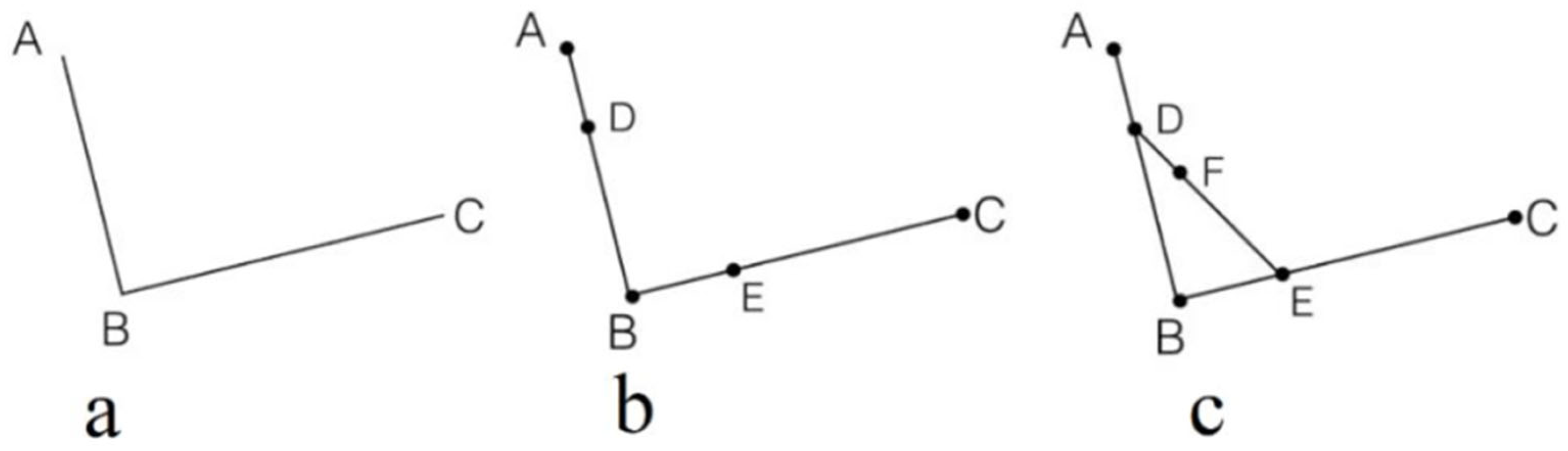
Here, P0, P1, and P2 represent the coordinates of the control points, and is the parameter varying from 0 to 1. The principle and steps of forming a second-order Bézier curve are illustrated in Figure 7.
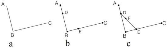
Figure 7.
Bézier curve formation process diagram. (a) Step one; (b) step two; (c) step three.
The working principle and drawing steps of a Bézier curve are as follows:
Step 1: Find three non-collinear points on a two-dimensional plane and connect them with line segments, as shown in Figure 7a;
Step 2: Find points D and E on line segments AB and BC, respectively, such that the ratios of AD to DB and BE to EC are equal, as shown in Figure 7b;
Step 3: Connect points D and E to form line segment DE. On segment DE, find point F such that the ratios of DF to FE, AD to DB, and BE to EC are all equal, as shown in Figure 7c;
Step 4: Find all coordinates that satisfy the conditions from steps 2 and 3 and connect them to form the curve, as shown in Figure 8.
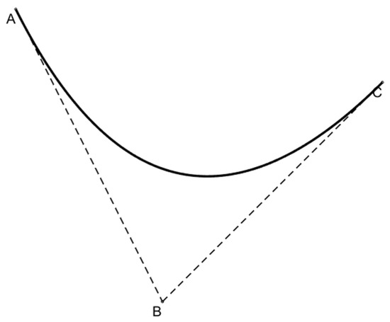
Figure 8.
Second-order Bezier curve.
It can be seen from Figure 8 and Equation (14) that the second-order Bézier curve is generated by three control points. The three control points can be three non-collinear position points on the curve, the initial position point, and the end position point of the curve, which overlaps the start and end points of the original curve.
In the Bézier curve smoothing algorithm, the order of the curve can be determined based on the number of inflection points within a segment of the curve. Therefore, it performs well in smoothing global paths, as Bézier curves excel at smoothing path curves. This capability significantly contributes to enhancing the overall operational lifespan of mobile robots [20].
- The Artificial Potential Field Method (APF) and its Optimization;
The artificial potential field method is a widely used approach in path planning, which abstracts the workspace of robots into a virtual force field. In this field, robots are subjected to two types of potential field forces: the goal potential field force and the obstacle potential field force. The goal potential field force refers to the attractive force exerted on the robot as it moves toward the target point, pulling the robot closer to the target. On the other hand, the obstacle potential field force represents the repulsive force experienced by the robot as it approaches obstacles, pushing the robot away from obstacles [21,22].
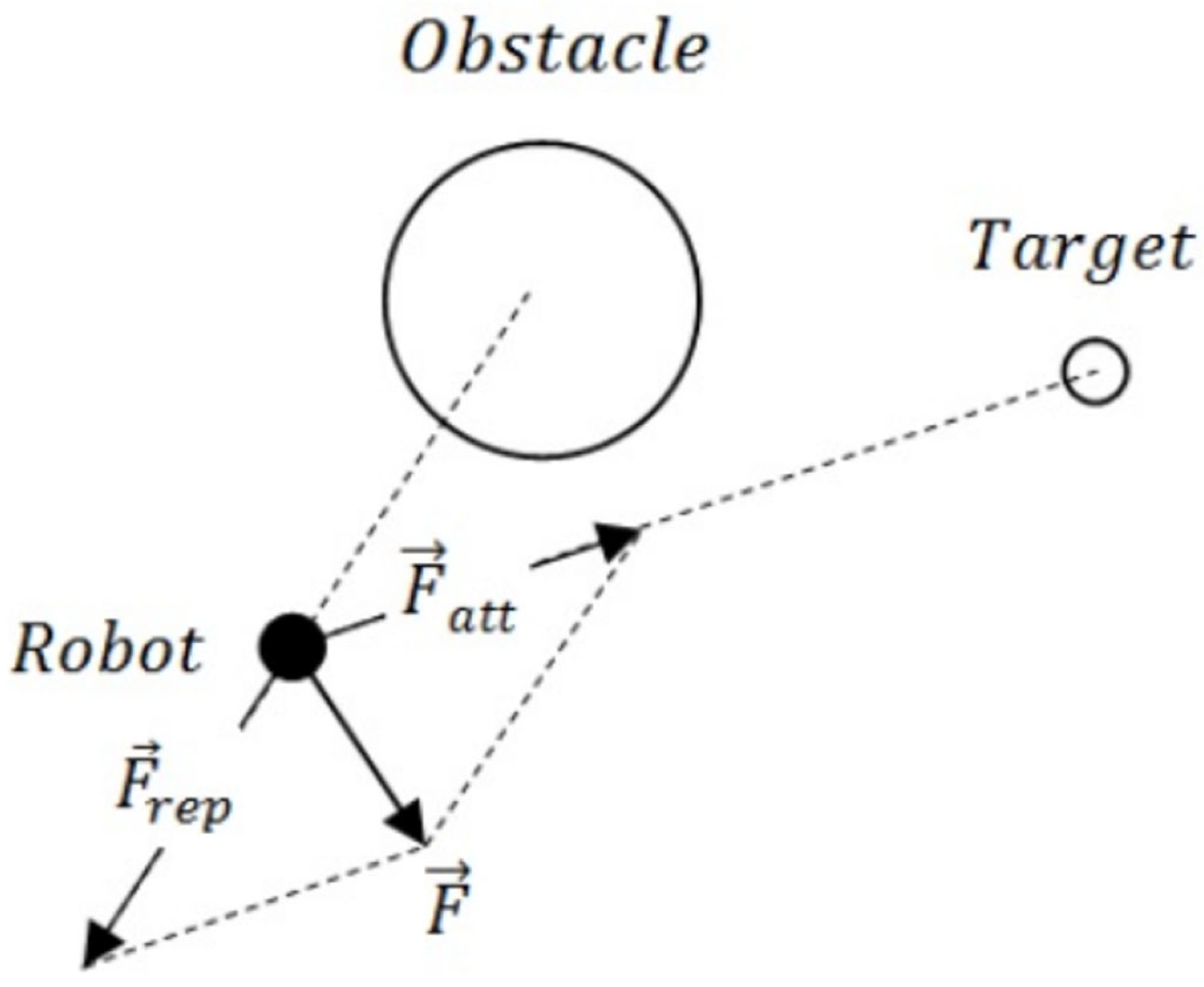
The schematic diagram of the artificial potential field method is illustrated in Figure 9, where denotes the repulsive force generated by the repulsive field, represents the attraction force generated by the attractive field, and denotes the resultant force acting on the robot. The coordinates of the robot’s position , the target point position , and the obstacle position are denoted as , , and , respectively. In the potential field, as the distance between the robot and the target increases, the attraction exerted by the target on the robot becomes stronger. Conversely, as the distance between the robot and the obstacle decreases, the repulsion exerted by the obstacle on the robot becomes stronger. Therefore, the attraction field and the repulsion field can be designed as follows, where the potential energy function for the attraction field is defined as:
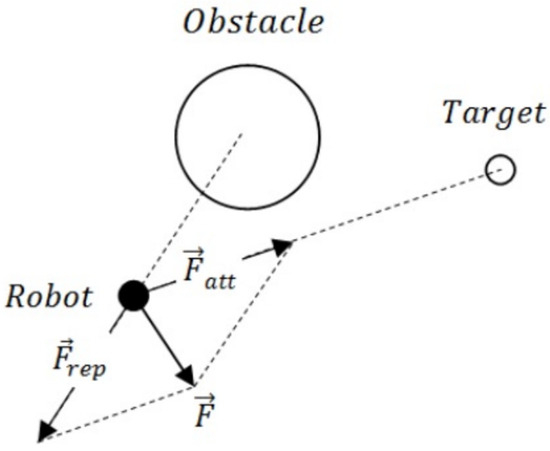
Figure 9.
Principle of artificial potential field method.
In the formula, is the gravitational field gain coefficient, is the distance between the robot and the target point.
Then, the gravitational force generated by the gravitational field is:
The repulsive field is generated by obstacles, and the repulsive field’s potential energy function is defined as:
Among them, is the repulsion field gain coefficient, is the distance between the robot and the obstacle, and is the repulsive force range.
Then, the repulsive force generated by the repulsive force field is:
The robot’s resultant potential field function is the vector superposition of the gravitational field function and the repulsion field function. The resultant potential field function can be expressed as:
The resultant force on the robot is:
Traditional artificial potential field methods have some drawbacks in robot path planning. When the resultant force acting on the robot, composed of both attraction and repulsion forces, equals zero, two possible scenarios arise: the robot may either remain stationary at its current position or oscillate around that position. Additionally, if the robot reaches the target point successfully but still experiences the effect of repulsive forces, it may fail to remain at the target point [23,24,25]. To address these issues, improvements can be made to the potential energy function of the repulsive field, as follows:
The improved repulsive field potential energy function introduces a control quantity . Compared with the traditional repulsive field potential energy function, this improved function makes 0 when the robot reaches the target point, and then makes also 0, thus satisfying the repulsive field potential energy when the robot reaches the target point. zero requirement. At this time, the repulsive force is the negative gradient of the improved repulsive field potential energy function:
In the formula: and are the two components of repulsion in the direction of gravity and repulsion respectively. Among them, is the gravitational component, and the specific calculation formula is:
is the repulsive force component. The specific calculation formula is:
It can be seen from the above that this improved method allows the robot to accurately reach the target point under the action of the gravitational component, and, at the same time, avoids collision with obstacles by gradually reducing the repulsive component. In this way, the robot is able to reach its target location in a stable and safe manner while avoiding potential collision risks [26,27,28].
- Algorithm combination process;
In order to realize the dynamic path planning design of mobile robots integrating the improved A* algorithm and the artificial potential field method, this paper first uses the improved A* algorithm to find the static optimal trajectory. Then, the static optimal trajectory is optimized through the n-order Bezier curve method, while redundant nodes are removed and special point angles are optimized to obtain the optimized static optimal trajectory. Next, in order to combine the A* algorithm with the artificial potential field method, it is necessary to discretize the optimal trajectory into trajectory points and create the gravitational potential energy field of the static optimal trajectory so that during the process of dynamic path planning, along the trajectory The line is used for obstacle avoidance and tracking, and is the gravity of each point on the trajectory. Finally, the fusion of the three algorithms is completed, which can achieve good path planning effects.
3. Experiments and Results
This article is mainly devoted to experimental analysis to verify the effectiveness of the proposed path-planning method. Experiment 1 will conduct a simulation experiment of the map preprocessing algorithm to evaluate the effectiveness of the algorithm in different scenarios. Experiment 2 will explore the influence of the parameters of the A* algorithm on the path planning results in order to gain an in-depth understanding of the working mechanism of the algorithm and optimize the parameter selection. The purpose of experiment 3 is to verify the advantages of the fusion of the improved A* algorithm and the artificial potential field method, to verify the degree of improvement of the fusion algorithm on the path planning results, and to conduct quantitative analysis through simulation experiments.
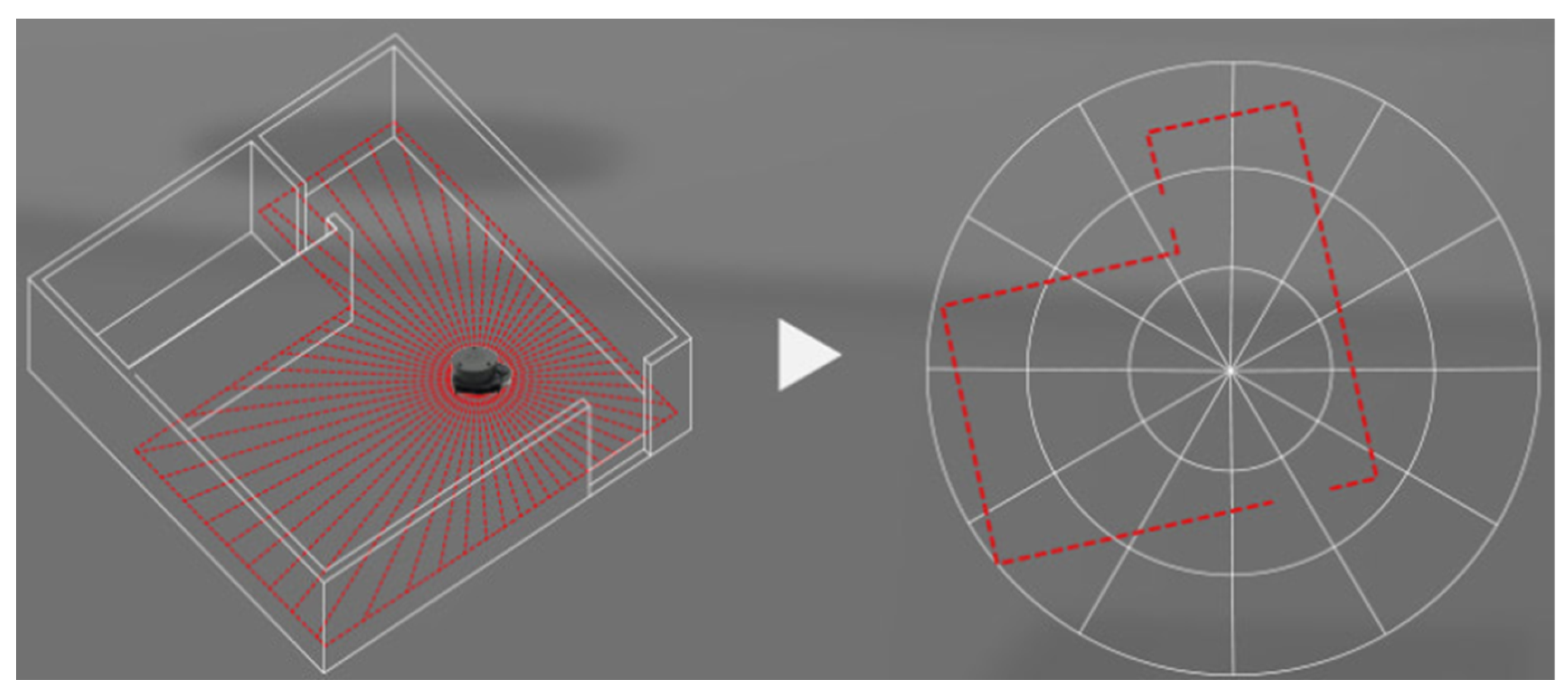
In the process of building the map in this article, there are two kinds of obstacles: static and dynamic, as shown in Figure 10. We need to use SLAM’s RPLidarA1 2D laser radar (Slamtec, Shanghai, China) as a sensor to collect surrounding information and to locate and measure distance. The scanning frequency range is 2–10 Hz. This sensor uses laser triangulation ranging technology, with a ranging frequency of more than 8000 times per second and a maximum measurement radius of 12 m. Using laser radar, we can build static obstacle models in the environment and detect dynamic obstacles in the environment during dynamic obstacle avoidance, meeting the requirements.

Figure 10.
Lidar scan map.
It is worth highlighting that the optimal path derived from the hybrid path planning approach in this paper must be symmetrical. This means that whether the path is traced from the starting point to the destination or vice versa, the outcomes of both experiments should be identical, featuring the same nodes and motion trajectories. While other individual algorithms may not satisfy the symmetry of the path (such as the APF algorithm), the hybrid algorithm presented in this paper can indeed fulfill the principle of symmetry. In the context of optimal trajectory determination, the verification of trajectory symmetry provides a straightforward and intuitive means to assess whether the experimental results are optimal. That is, the optimal trajectory should be symmetrical.
3.1. Experiment 1: Map Preprocessing Optimization Experiment
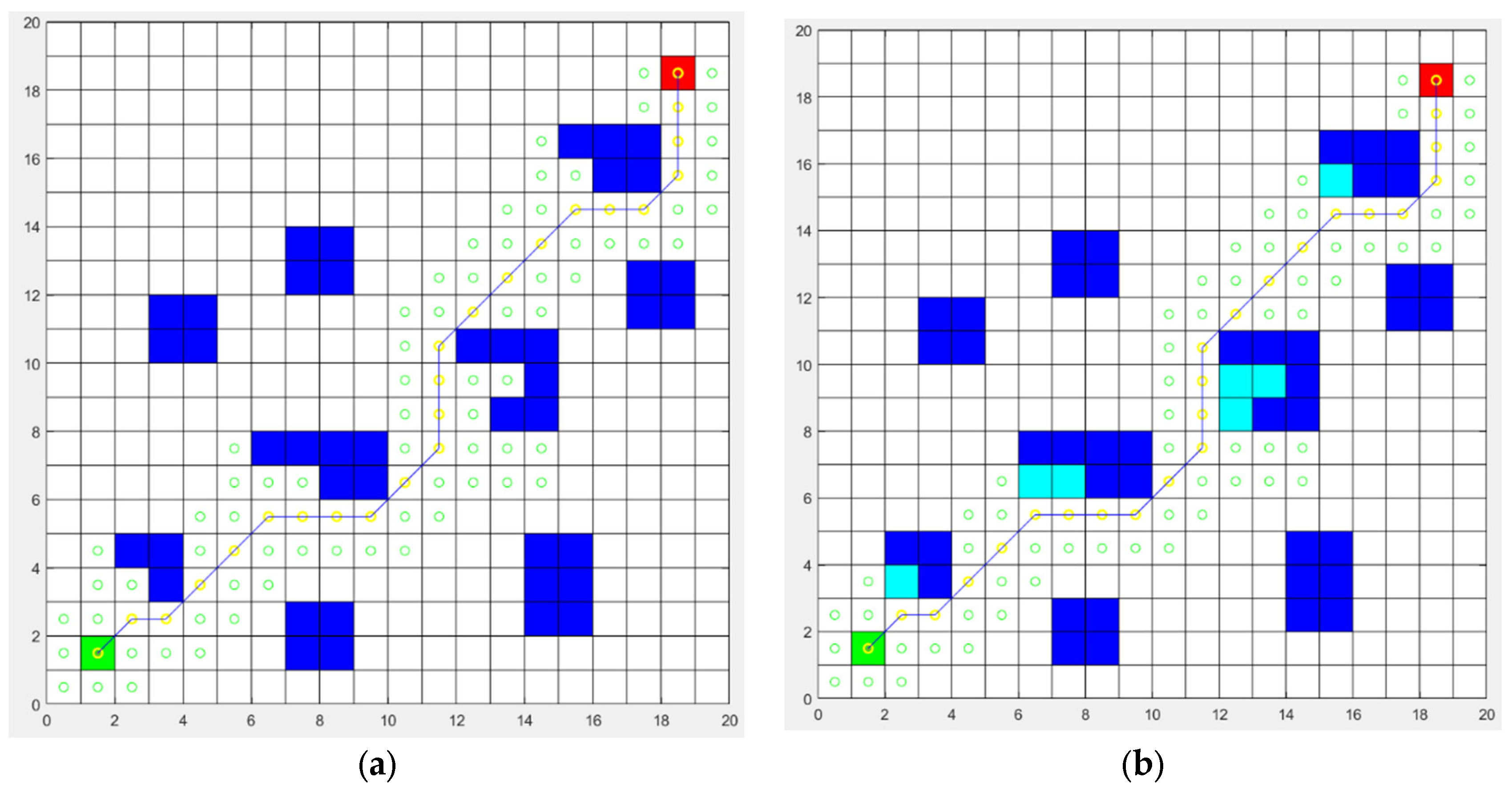
Taking the A* algorithm search as an example, the effect of this map preprocessing algorithm is analyzed [29,30,31]. Among them, the green circle represents all child nodes in the search process, while the yellow circle represents the final selected target node. The path searched by the A*algorithm is marked with a solid blue line. Through the preprocessing of the grid map, a new obstacle grid with a light blue background was introduced, and then the A* algorithm was used again for path planning.
First of all, we analyze the first case. The result of the unoptimized processing is shown in Figure 11a, while the result of the preprocessing of the grid map is shown in Figure 11b. Although the pathfinding result is still presented as a solid black line path, after preprocessing the grid map, the search result of the A algorithm has actually changed. Although there is no difference in appearance, a new obstacle grid has been introduced in the map during the preprocessing phase. These obstacles may also cause the A* algorithm to choose different paths during the search process. Even if the result path looks the same, the preprocessing stage still has an impact on the search of the A* algorithm. Next, we will conduct further analysis.
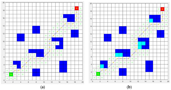
Figure 11.
Comparison of search results before and after adding map preprocessing. (a) A* algorithm search results for unprocessed maps; (b) A* algorithm search results for processed maps.
The relevant information of the two results is counted, as shown in Table 1 below.

Table 1.
Comparison of results.
It can be obtained through the data analysis in Table 1. Although the front and rear paths are the same, in the two dimensions of search node and search time, the number of pre-processed map search nodes has been reduced by 11.6%, and the search time has been reduced by 18.6%. The main reason for this difference is that there is a concave obstacle in Figure 11. The A* algorithm has to enter the interior of the concave obstacle to search during path planning. This is an unavoidable feature of the A* algorithm.
In Figure 11, the A* algorithm performs a path search at the filled light blue square and its surrounding nodes, but the search at these locations does not help in the discovery of valid paths, so it is an invalid search. In contrast, when the A* algorithm is used for path search after preprocessing the grid map, the search process is shown in Figure 11b. Due to the addition of virtual obstacles, the internal area of the concave obstacles is filled, so the path search will not enter the interior of the concave obstacles, thereby saving the search work for these locations. Although the search results are still the same path curve, the search efficiency is significantly improved with the assistance of the grid map preprocessing algorithm.
Through the above analysis, it can be inferred that with the increase of the scale of the map and the number of obstacles, the path search effect after map preprocessing will be further improved [32,33].
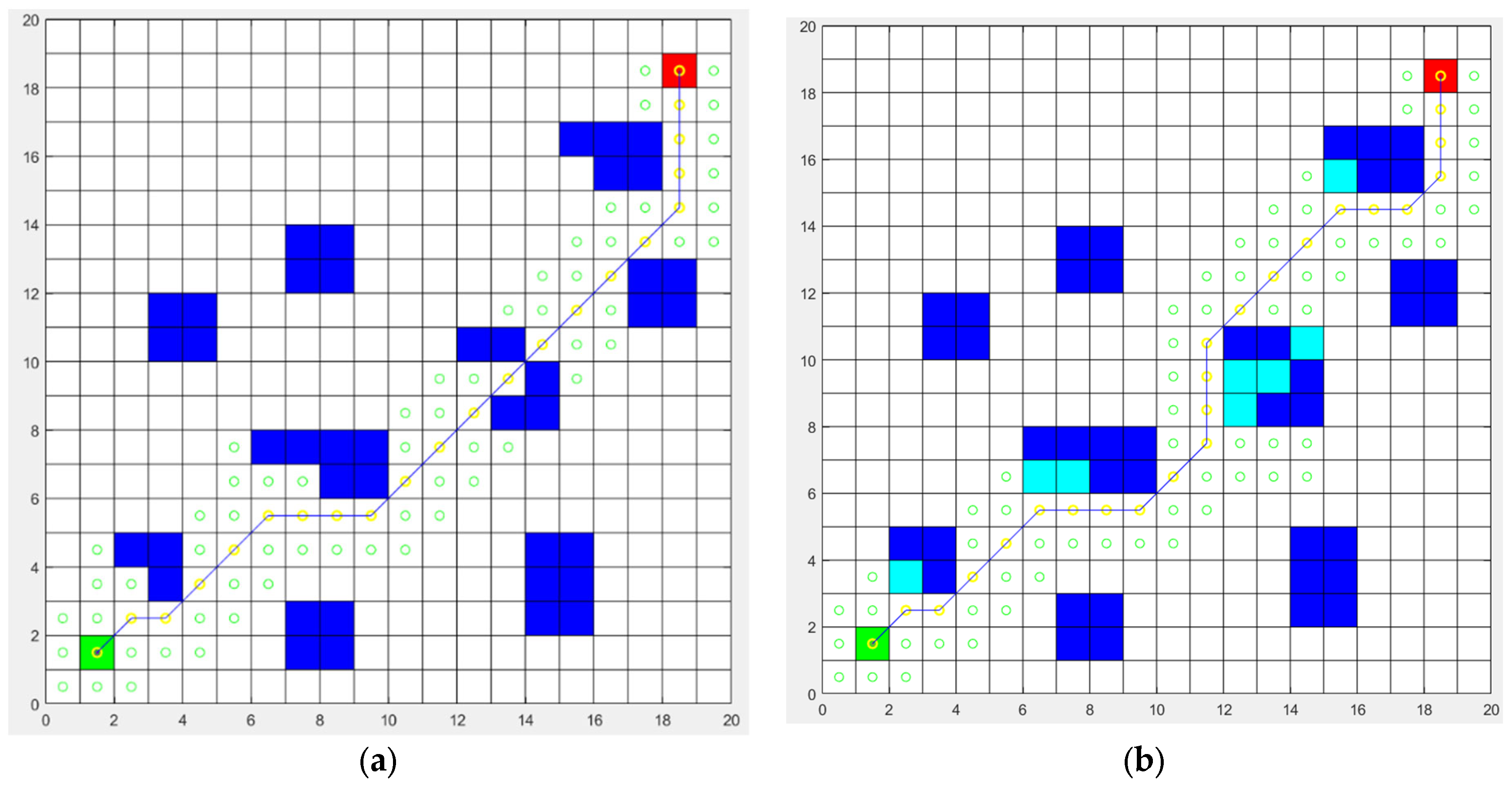
In the second case, we deleted the obstacles (15, 11), observed the results of the path search, and compared the trajectories without map preprocessing and map preprocessing, respectively. The result is shown in Figure 12. Without map preprocessing, the trajectory is shown in Figure 12a, and it is found that an error occurred in the process from the square coordinates (14, 10) to (15, 11). This is because, in the case of an eight-field search, it is impossible to identify the problem that the diagonal coordinate position is unreachable under special circumstances. Due to the robot’s own volume problem, in practical applications, the robot cannot move from the square coordinates (14, 10) to (15, 11). Therefore, this problem needs to be solved in the algorithm design to avoid the algorithm from failing under certain circumstances. The results of the map preprocessing are shown in Figure 12b, which can avoid the problem of diagonal position failure.

Figure 12.
Comparison of search results before and after removing specific obstacles. (a) No map preprocessing after removing a specific obstacle; (b) map preprocessing after removing a specific obstacle.
The map preprocessing algorithm in this paper mainly aims to solve two types of potential problems. First of all, the statically observed map itself may have defects, such as obstacles that are not correctly marked or obstacles that cannot be traversed by the robot not being accurately handled. These problems may cause the path-planning algorithm to fail in practical applications. Secondly, there may be a large number of invalid nodes in the path search process. These nodes are not conducive to the effective operation of the search algorithm and will increase the time complexity of the search. Therefore, the map preprocessing algorithm is designed to remove invalid nodes in the map and optimize the structure of the map, thereby improving the efficiency and accuracy of the path search algorithm.
3.2. Experiment 2: A* Algorithm Parameter Analysis
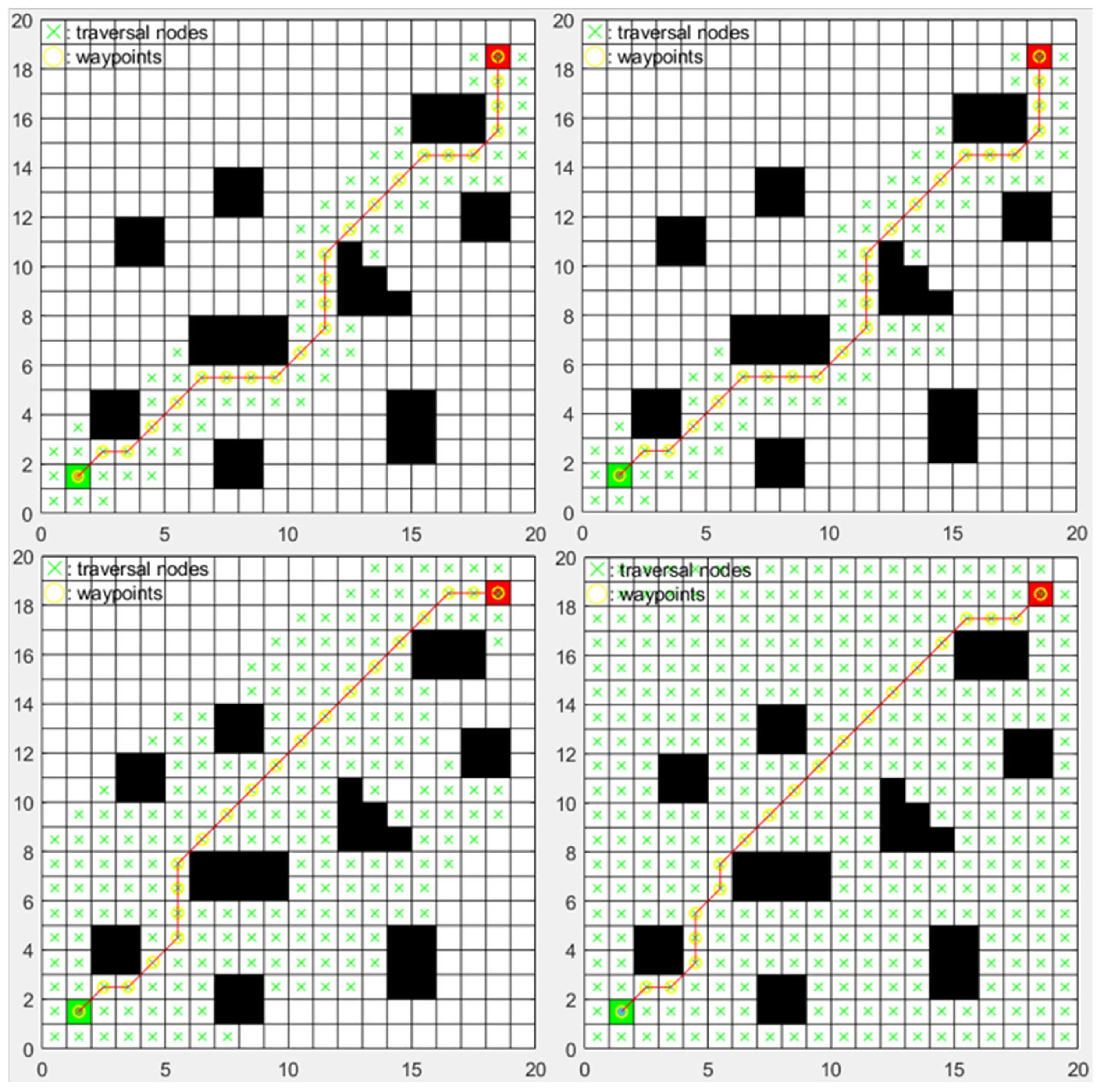
Due to the theoretically higher precision of Euclidean distance compared to Manhattan distance and Chebyshev distance, this experiment adopts Euclidean distance calculation. To investigate the influence of weighting coefficients of the heuristic function on the search nodes, different weighting coefficients are selected as 0, 0.5, 0.75, and 1 for simulation experiments. The obtained results are depicted in Figure 13, corresponding to values of 0, 0.5, 0.75, and 1, respectively. The summarized data are presented in Table 2.
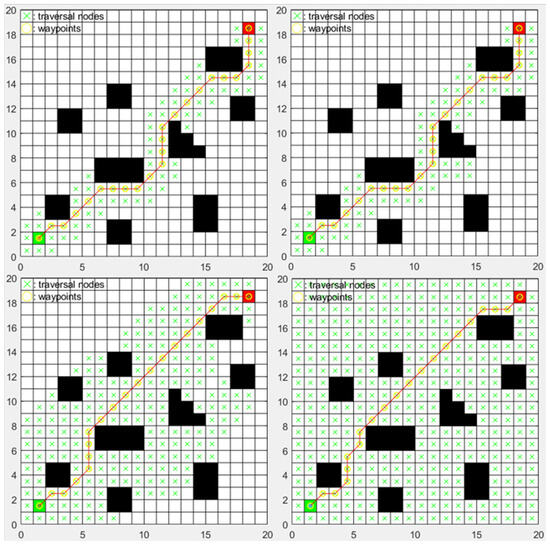
Figure 13.
The effect diagram when the weight coefficient w increases.
Table 2.
Experiment 2 data summary table.
The figure shows the change in the number of nodes searched by the A* algorithm when w is (0, 0.5, 0.75, 1).
Based on the data analysis, the following conclusions can be drawn as the weight of in the estimation function increases, the time consumption for searching increases, and the search scope expands, leading to paths closer to the global optimum. Conversely, as the weight decreases, the search time shortens, and the search scope narrows, but it does not necessarily guarantee the global optimum path. In order to strike a balance between search speed and search scope, this study chooses to be 0.5.
3.3. Experiment 3: Simulation Analysis of Hybrid Path Planning
Using the simulation environment used in this article, consistent map obstacle information is used to set the same starting and target points and observe the mixed dynamic planning effect in the static obstacle environment and the presence of the dynamic obstacle environment, respectively. For comparison, only the improved artificial potential field method of this paper is used for planning, and the hybrid algorithm is used for planning. The effect of path planning is different. At the same time, two moving objects (red spheres) are introduced. Object 1 moves up and down between the three units of the square (6, 3–5), and object 2 moves left and right between the five units of the square (13–17, 14) to verify the dynamic obstacle avoidance effect. In order to compare the experimental results, the simulation parameters of the algorithm are unified, and the experimental parameters are shown in Table 3.
Table 3.
Experimental parameters.
According to the results shown in Figure 14 and Figure 15, the path planning performance of the hybrid algorithm in the same environment is significantly better than that of the path planning using only the improved artificial potential field method, which is mainly reflected in the smoothness and stability of the path. Through the hybrid algorithm, the oscillation phenomenon in the path is successfully reduced, and the path is smoothed. In addition, the hybrid algorithm first uses the global planning method to obtain the initial path, avoiding the one-sided problem of environmental recognition that may arise when only local path planning is used. By setting sub-goals, the hybrid algorithm has also achieved remarkable results in reducing the path planning time, reducing the computational complexity of the robot, and improving the planning efficiency, further verifying the theoretical analysis of the previous article.
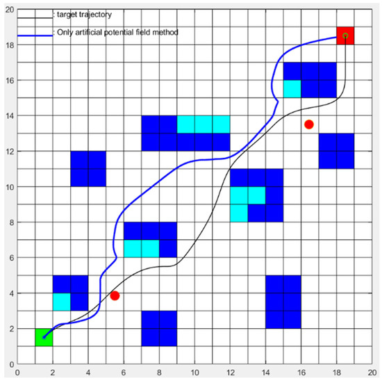
Figure 14.
Comparison of separate APF algorithm and A* algorithm.

Figure 15.
Hybrid algorithm in static maps and dynamic maps. (a) Static map; (b) dynamic map.
In a static environment, the improved A algorithm has been able to effectively plan the shortest and smooth path, and the calculation time is relatively short. Compared with the improved A algorithm, the path obtained by the hybrid algorithm is basically the same. Although there may be slight oscillations in the local path planning process, it does not affect the smoothness of the overall path. Considering that the hybrid algorithm is mainly to solve the limitations of the improved A* algorithm in a dynamic environment, in a static environment, the path generated by the hybrid algorithm can still meet the work requirements, indicating its applicability in a static environment. Through the verification in Figure 14 and Figure 15, we found that the hybrid path planning algorithm is better than the separate A* algorithm and APF algorithm in many aspects. First, compared with the path generated by the A* algorithm, the hybrid path planning algorithm can find the optimal path to ensure the symmetry of the path. Secondly, the hybrid path planning algorithm can adapt to the dynamic environment and maintain a safe distance from obstacles, thus greatly improving the practicality of the algorithm. These advantages make hybrid path planning algorithms more efficient and reliable in practical applications.
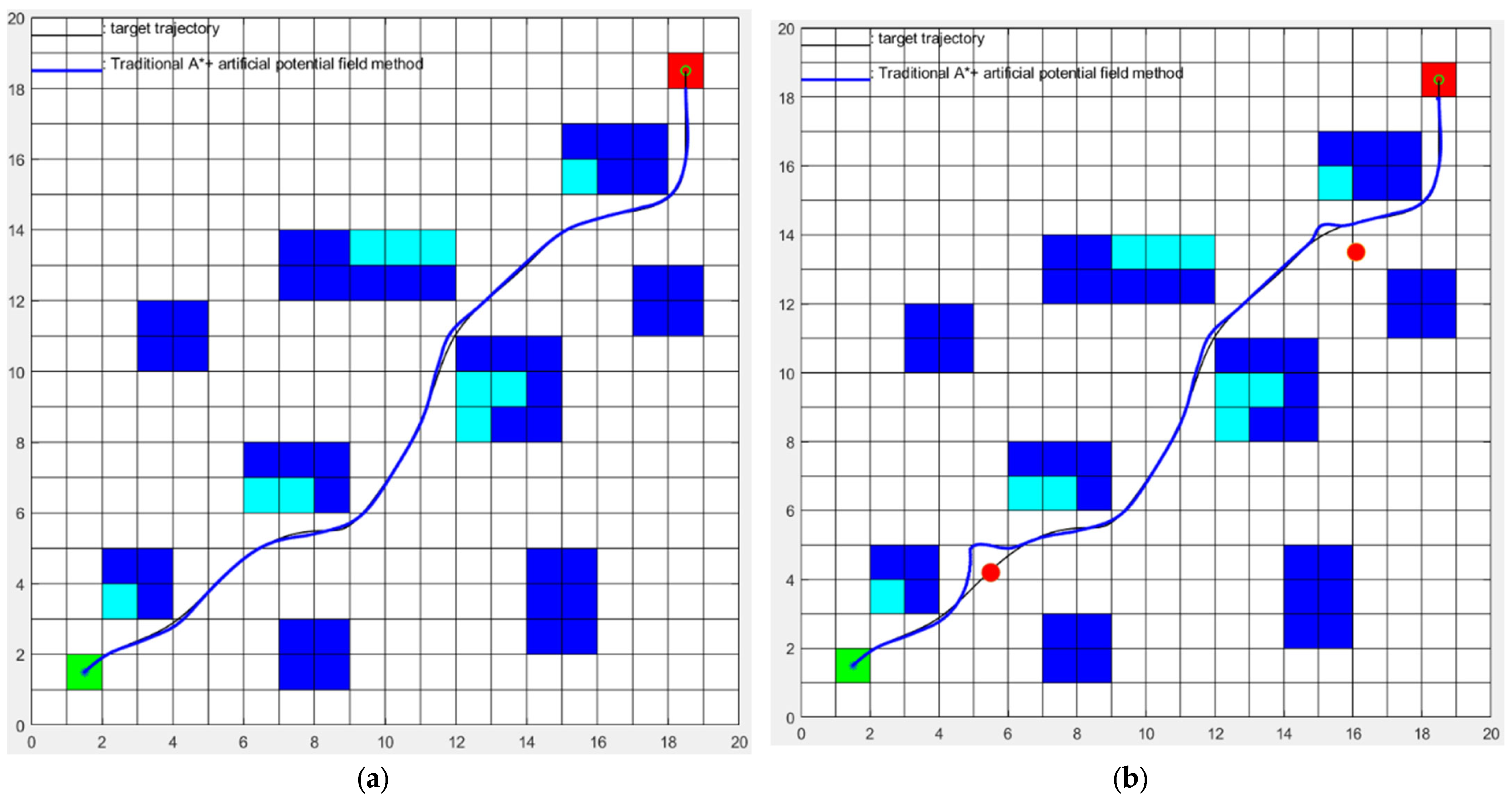
Figure 16 is the comparison result between the proposed algorithm and the Ref. [34] algorithm in static maps. As shown in Table 4, we can intuitively find that the number of search nodes of the proposed fusion algorithm is significantly lower than that of the Ref. [34] algorithm. The data in Table 4 show that when the trajectory length is basically the same, the proposed algorithm greatly improves the search efficiency and reduces the time by 216%. In addition, it can be found from Figure 16b that the proposed algorithm is still effective in complex environments with dynamic obstacles.
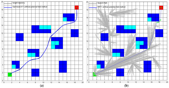
Figure 16.
Comparison between the algorithm in this paper and the algorithm in Ref. [34]. (a) The algorithm in this paper; (b) the algorithm in Ref. [34].
Table 4.
Comparison between the proposed algorithm and the Ref. [34] algorithm under static map.
Through the experiments, we can draw the following conclusions: the map preprocessing algorithm proposed in this paper can significantly improve the search efficiency, eliminate unreachable and unnecessary nodes, and reduce the search time. By changing the weight coefficient w of the A* algorithm, the search process and results can be significantly changed. The fusion algorithm in this paper optimizes the defects of the A* algorithm and the artificial potential field method and combines the advantages of both. It can achieve mobile robot navigation and obstacle avoidance in complex environments. The comparison with the literature [34] highlights that the new algorithm proposed in this paper has significant advantages, being faster, more efficient, and requiring fewer calculations.
4. Discussion
Autonomous path-planning technology for mobile robots is one of the core technologies widely applied in various fields [35]. This study addresses the path-planning problem of mobile robots in complex environments with dynamic and unknown obstacles. Research is conducted from three aspects: global path planning, local path planning, and hybrid path planning. The effectiveness of the research content is validated through simulation experiments. The specific research achievements are as follows:
- In this study, a method of preprocessing grid maps is proposed to improve the efficiency of path planning and optimize path results. This method encloses the internal space of concave obstacles, which can effectively reduce the number of grid nodes searched by the A* algorithm during path planning, thereby improving the efficiency of path search. It also effectively solves the practical application problems caused by the robot’s own volume problem in path planning, such as the situation where the diagonal position is unreachable. Through this preprocessing method, a more reliable map foundation can be provided in the global path planning and local path planning stages, and it is expected to achieve more efficient and optimized path planning;
- For the issues in the A* algorithm used for global path planning, such as excessive node traversal, low search efficiency, redundant path nodes, and non-smooth turning angles, an improved heuristic function and weight coefficients are proposed. Additionally, the n-order Bézier curve method is introduced for trajectory optimization and removal of redundant nodes. Simulation results demonstrate that the improved algorithm outperforms the A* algorithm in terms of planning efficiency, number of turns, path smoothness, and path length;
- Regarding the problems in the artificial potential field method used for local path planning, including local minima and unreachable target points, an improved artificial potential field method is proposed. It combines with the A* algorithm to optimize trajectories and eliminate local minima and unreachable target points. Simulation results show that the proposed algorithm not only successfully solves the problems of local minima and unreachable target points but also achieves a higher planning success rate, shorter average path length, shorter planning time, and lower total turning angle;
- Considering the limitations of global path planning algorithms in dynamic environments and the tendency of local path planning algorithms to fall into local minima, a hybrid path planning algorithm based on the A* algorithm and artificial potential field method is proposed. This algorithm utilizes the A* algorithm to plan the globally optimal path and then conducts Bézier curve optimization and designs the gravitational potential field for the tracking effect. Meanwhile, it employs the improved artificial potential field for local dynamic obstacle avoidance. Simulation results demonstrate that the proposed hybrid algorithm effectively addresses the issues of global path planning algorithms’ inability to dynamically avoid obstacles and local path planning algorithms’ susceptibility to local minima.
The innovation of this paper is mainly reflected in the proposal of a new map preprocessing method, which improves the search efficiency, makes its own improvement on the A* algorithm and the artificial potential field method, and proposes a new algorithm combination method and fusion algorithm. The final hybrid algorithm can meet the requirements of trajectory planning and obstacle avoidance in complex environments, and its efficiency can surpass most of the current path-planning methods. Its main features are high efficiency and light weight.
This paper addresses the challenges in real-time performance and dynamic obstacle avoidance capabilities of mobile robot path planning algorithms. Research is conducted on global path planning, local path planning, and hybrid path planning algorithms, and the effectiveness of the proposed algorithms is verified through map environment construction and simulation experiments, demonstrating their superiority over other algorithms. However, there are still some issues that need further research and improvement, including the following:
- The algorithms proposed in this paper are only designed for single robots and do not consider coordination and obstacle avoidance among multiple robots. Therefore, future research efforts could focus on the coordination of multiple robots and the optimization of obstacle avoidance strategies in multi-robot scenarios;
- This paper primarily addresses the obstacle avoidance problem in two-dimensional plane environments and does not account for variations in ground elevation. To better reflect real-world applications, further research is needed to investigate the complexity of ground environments and extend the scope of study to three-dimensional spaces.
5. Conclusions
In this study, in response to the issues of low search efficiency, redundant path nodes, non-smooth path turning angles, and the tendency to fall into local optima in traditional A* algorithms and artificial potential field methods, we have improved the heuristic function of the A* algorithm to enhance search efficiency. A new global path planning algorithm has been proposed to reduce redundant path nodes. The Bezier algorithm has been utilized to optimize the smoothness of the trajectory, and the repulsive function of the artificial potential field method has been improved to make the target point the global minimum of potential energy, thereby solving the problem of robots being trapped in local optima. Finally, based on the A* algorithm and the artificial potential field method, a new hybrid algorithm has been proposed that combines the advantages of both.
In the design of the hybrid algorithm presented in this paper, initial steps were taken to preprocess and optimize the global map, preparing for subsequent global path planning. Subsequently, the optimized global path planning algorithm, A*, was utilized to obtain the globally optimal path. Considering the physical characteristics of mobile robot movement, the Bezier optimization algorithm was introduced to enhance the smoothness of the trajectory. On the basis of the globally optimal trajectory, the path was segmented, and the artificial potential field method was employed to enable dynamic obstacle avoidance while navigating the path. Finally, a fusion algorithm was designed to integrate the A* algorithm and the artificial potential field method, completing the design of the entire hybrid algorithm.
After simulation experiments and comparisons with algorithms in the literature, the search range of our algorithm has been significantly reduced in the simulation scenario. In terms of search time, the search efficiency has increased by up to 216%, and the length of the search path has been slightly optimized. Therefore, the hybrid algorithm proposed in this paper, based on the A* algorithm and the artificial potential field method, can effectively improve the efficiency and smoothness of path planning, providing a high-efficiency, lightweight, and reliable algorithm for the trajectory planning of mobile robots under complex conditions.
Author Contributions
Conceptualization, Y.K.; Methodology, R.Y.; Software, Y.K. and R.Y.; Validation, Y.K.; Formal analysis, R.Y.; Investigation, Y.K.; Resources, R.Y.; Data curation, Y.K. and R.Y.; Writing—original draft, Y.K. and R.Y. All authors have read and agreed to the published version of the manuscript.
Funding
This research received no external funding.
Data Availability Statement
Data are contained with the article.
Conflicts of Interest
The authors declare no conflicts of interest.
References
- Cai, X.; Ning, H.; Dhelim, S.; Zhou, R.; Zhang, T.; Xu, Y.; Wan, Y. Robot and its living space: A roadmap for robot development based on the view of living space. Digit. Commun. Netw. 2021, 7, 505–517. [Google Scholar] [CrossRef]
- Fu, B.; Chen, L.; Zhou, Y.; Zheng, D.; Wei, Z.; Dai, J.; Pan, H. An improved A* algorithm for the industrial robot path planning with high success rate and short length. Robot. Auton. Syst. 2018, 106, 26–37. [Google Scholar] [CrossRef]
- Regev, C.; Jiang, Z.; Kasher, R.; Miller, Y. Distinct Antifouling Mechanisms on Different Chain Densities of Zwitterionic Polymers. Molecules 2022, 27, 7394. [Google Scholar] [CrossRef] [PubMed]
- Guo, Y.; Yang, Y.; Liu, Y.; Li, Q.; Cao, F.; Feng, M.; Wu, H.; Li, W.; Kang, Y. Development Status and Multilevel Classification Strategy of Medical Robots. Electronics 2021, 10, 1278. [Google Scholar] [CrossRef]
- Islamov, S.; Grigoriev, A.; Beloglazov, I.; Savchenkov, S.; Gudmestad, O.T. Research Risk Factors in Monitoring Well Drilling—A Case Study Using Machine Learning Methods. Symmetry 2021, 13, 1293. [Google Scholar] [CrossRef]
- Vaussard, F.; Fink, J.; Bauwens, V.; Rétornaz, P.; Hamel, D.; Dillenbourg, P.; Mondada, F. Lessons learned from robotic vacuum cleaners entering the home ecosystem. Robot. Auton. Syst. 2014, 62, 376–391. [Google Scholar] [CrossRef]
- Zhukovskiy, Y.L.; Kovalchuk, M.S.; Batueva, D.E.; Senchilo, N.D. Development of an Algorithm for Regulating the Load Schedule of Educational Institutions Based on the Forecast of Electric Consumption within the Framework of Application of the Demand Response. Sustainability 2021, 13, 13801. [Google Scholar] [CrossRef]
- Ajeil, F.H.; Ibraheem, I.K.; Sahib, M.A.; Humaidi, A.J. Multi-objective path planning of an autonomous mobile robot using hybrid PSO-MFB optimization algorithm. Appl. Soft Comput. 2020, 89, 106076. [Google Scholar] [CrossRef]
- Qing, G.; Zheng, Z.; Yue, X. Path-planning of automated guided vehicle based on improved Dijkstra algorithm. In Proceedings of the 2017 29th Chinese Control and Decision Conference (CCDC), Chongqing, China, 28–30 May 2017; pp. 7138–7143. [Google Scholar]
- Beloglazov, I.I.; Plaschinsky, V.A. Development MPC for the Grinding Process in SAG Mills Using DEM Investigations on LinerWear. Materials 2024, 17, 795. [Google Scholar] [CrossRef]
- Enayattabar, M.; Ebrahimnejad, A.; Motameni, H. Dijkstra algorithm for shortest path problem under interval-valued Pythagorean fuzzy environment. Complex Intell. Syst. 2019, 5, 93–100. [Google Scholar] [CrossRef]
- Song, B.; Wang, Z.; Zou, L. An improved PSO algorithm for smooth path planning of mobile robots using continuous high-degree Bezier curve. Appl. Soft Comput. 2021, 100, 106960. [Google Scholar] [CrossRef]
- Brigadnov, I.; Lutonin, A.; Bogdanova, K. Error State Extended Kalman Filter Localization for Underground Mining Environments. Symmetry 2023, 15, 344. [Google Scholar] [CrossRef]
- Zhang, H.-M.; Li, M.-L.; Yang, L. Safe Path Planning of Mobile Robot Based on Improved A* Algorithm in Complex Terrains. Algorithms 2018, 11, 44. [Google Scholar] [CrossRef]
- Pandini, M.M.; Spacek, A.D.; Neto, J.M.; Ando, O. Design of a Didatic Workbench of Industrial Automation Systems for Engineering Education. IEEE Lat. Am. Trans. 2017, 15, 1384–1391. [Google Scholar] [CrossRef]
- Yang, D.; Xu, B.; Rao, K.; Sheng, W. Passive Infrared (PIR)-Based Indoor Position Tracking for Smart Homes Using Accessibility Maps and A-Star Algorithm. Sensors 2018, 18, 332. [Google Scholar] [CrossRef]
- Zhukovskiy, Y.L.; Koshenkova, A.A.; Vorobieva, V.A.; Raspunin, D.L. Assessment of the Impact of Technological Development and Scenario Forecasting of the Sustainable Development of the Fuel and Energy Complex. Energies 2023, 16, 3185. [Google Scholar] [CrossRef]
- Orozco-Rosas, U.; Montiel, O.; Sepúlveda, R. Mobile robot path planning using membrane evolutionary artificial potential field. Appl. Soft Comput. 2019, 77, 236–251. [Google Scholar] [CrossRef]
- Doostie, S.; Hoshiar, A.; Nazarahari, M.; Lee, S.; Choi, H. Optimal path planning of multiple nanoparticles in continuous environment using a novel Adaptive Genetic Algorithm. Precis. Eng. 2018, 53, 65–78. [Google Scholar] [CrossRef]
- Lamini, C.; Benhlima, S.; Elbekri, A. Genetic Algorithm Based Approach for Autonomous Mobile Robot Path Planning. Procedia Comput. Sci. 2018, 127, 180–189. [Google Scholar] [CrossRef]
- Zakharov, L.; Martyushev, D.; Ponomareva, I.N. Predicting dynamic formation pressure using artificial intelligence methods. J. Min. Inst. 2022, 253, 23–32. [Google Scholar] [CrossRef]
- Li, K.; Hu, Q.; Liu, J. Path planning of mobile robot based on improved multi-objective genetic algorithm. Wirel. Commun. Mob. Comput. 2021, 2021, 8836615. [Google Scholar] [CrossRef]
- Candeloro, M.; Lekkas, A.M.; Sørensen, A.J. A Voronoi-diagram-based dynamic path-planning system for underactuated marine vessels. Control. Eng. Pr. 2017, 61, 41–54. [Google Scholar] [CrossRef]
- Matrokhina, K.V.; Trofimets, V.Y.; Mazakov, E.B.; Makhovikov, A.B.; Khaykin, M.M. Development of methodology for scenario analysis of investment projects of enterprises of the mineral resource complex. J. Min. Inst. 2023, 259, 112–124. [Google Scholar] [CrossRef]
- Li, Y.; Zhao, J.; Chen, Z.; Xiong, G.; Liu, S. A Robot Path Planning Method Based on Improved Genetic Algorithm and Improved Dynamic Window Approach. Sustainability 2023, 15, 4656. [Google Scholar] [CrossRef]
- Filippov, V.; Zakharov, L.A.; Martyushev, D.A.; Ponomareva, I.N. Reproduction of reservoir pressure by machine learning methods and study of its influence on the cracks formation process in hydraulic fracturing. J. Min. Inst. 2022, 258, 924–932. [Google Scholar] [CrossRef]
- Wang, D.; Liu, Z.; Tao, Y.; Chen, W.; Chen, B.; Wang, Q.; Yan, X.; Wang, G. Improvement in EEG Source Imaging Accuracy by Means of Wavelet Packet Transform and Subspace Component Selection. IEEE Trans. Neural Syst. Rehabil. Eng. 2021, 29, 650–661. [Google Scholar] [CrossRef]
- Sychev, Y.; Zimin, R. Improving the quality of electricity in the power supply systems of the mineral resource complex with hybrid filter-compensating devices. J. Min. Inst. 2021, 247, 132–140. [Google Scholar] [CrossRef]
- Kozhubaev, Y.; Belyaev, V.; Murashov, Y.; Prokofev, O. Controlling of Unmanned Underwater Vehicles Using the Dynamic Planning of Symmetric Trajectory Based on Machine Learning for Marine Resources Exploration. Symmetry 2023, 15, 1783. [Google Scholar] [CrossRef]
- Muniteja, M.; Bee, M.K.M.; Suresh, V. Detection and classification of Melanoma image of skin cancer based on Convolutional Neural Network and comparison with Coactive Neuro Fuzzy Inference System. In Proceedings of the 2022 International Conference on Cyber Resilience (ICCR), Dubai, United Arab Emirates, 6–7 October 2022; pp. 1–5. [Google Scholar]
- Sychev, Y.A.; Aladin, M.E.; Aleksandrovich, S.V. Developing a hybrid filter structure and a control algorithm for hybrid power supply. Int. J. Power Electron. Drive Syst. 2022, 13, 1625–1634. [Google Scholar] [CrossRef]
- Alqobali, R.; Alshmrani, M.; Alnasser, R.; Rashidi, A.; Alhmiedat, T.; Alia, O.M. A Survey on Robot Semantic Navigation Systems for Indoor Environments. Appl. Sci. 2024, 14, 89. [Google Scholar] [CrossRef]
- Nowakowski, M.; Kurylo, J.; Braun, J.; Berger, G.S.; Mendes, J.; Lima, J. Using LiDAR Data as Image for AI to Recognize Objects in the Mobile Robot Operational Environment. In Optimization, Learning Algorithms and Applications; Pereira, A.I., Mendes, A., Fernandes, F.P., Pacheco, M.F., Coelho, J.P., Lima, J., Eds.; OL2A 2023. Communications in Computer and Information Science; Springer: Cham, Switzerland, 2024; Volume 1982. [Google Scholar] [CrossRef]
- Miao, H.; Chen, J.; Qi, B.; Li, Y.; Li, C. Path planning algorithm based on improved RRT and artificial potential field method. Autom. Instrum. 2023, 9–14. [Google Scholar] [CrossRef]
- Kramer, J.; Scheutz, M. Development environments for autonomous mobile robots: A survey. Auton. Robot. 2007, 22, 101–132. [Google Scholar] [CrossRef]


Disclaimer/Publisher’s Note: The statements, opinions and data contained in all publications are solely those of the individual author(s) and contributor(s) and not of MDPI and/or the editor(s). MDPI and/or the editor(s) disclaim responsibility for any injury to people or property resulting from any ideas, methods, instructions or products referred to in the content. |
© 2024 by the authors. Licensee MDPI, Basel, Switzerland. This article is an open access article distributed under the terms and conditions of the Creative Commons Attribution (CC BY) license (https://creativecommons.org/licenses/by/4.0/).