
Asymmetry Considerations in Constructing Control Charts: When Symmetry Is Not the Norm


Abstract
1. Introduction
2. Literature Review
3. Notations
4. Basic Assumptions
- (1)
- (2)
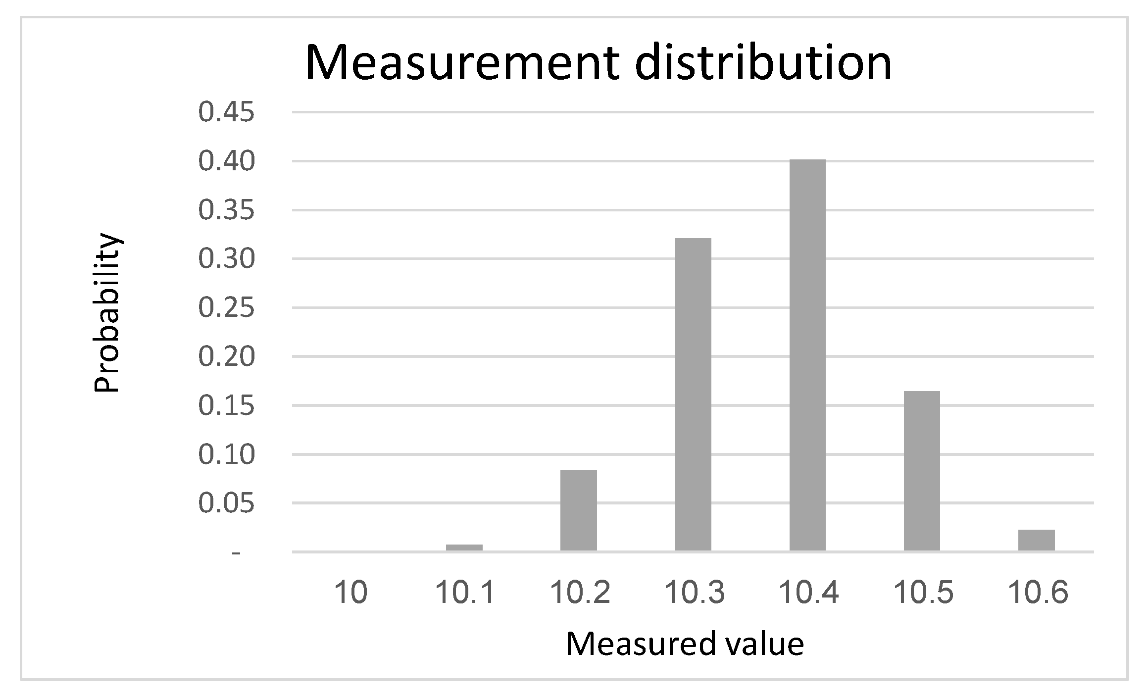
- Resolution impact—The observed value (denoted ) is rounded off to the nearest observable value. For example, if the resolution is °C, a value of 20.52 °C will be rounded off to 20.5 °C and a value of 20.57 °C will be rounded off to 20.6 °C. This assumption is the core of this research and was not introduced in previous research in this field.
- (3)
- Initial parameter measuring—The “exact” value of the mean and the variance of the measurand can be measured “accurately” (i.e., with high enough resolution). This can be achieved by either using exact measuring devices (applicable during the initial setting of the control limits, but not during the run off of the production process) or using the methods suggested by Gertsbakh and Benson-Karhi [20,38]. This assumption is well established in recent research.
- (4)
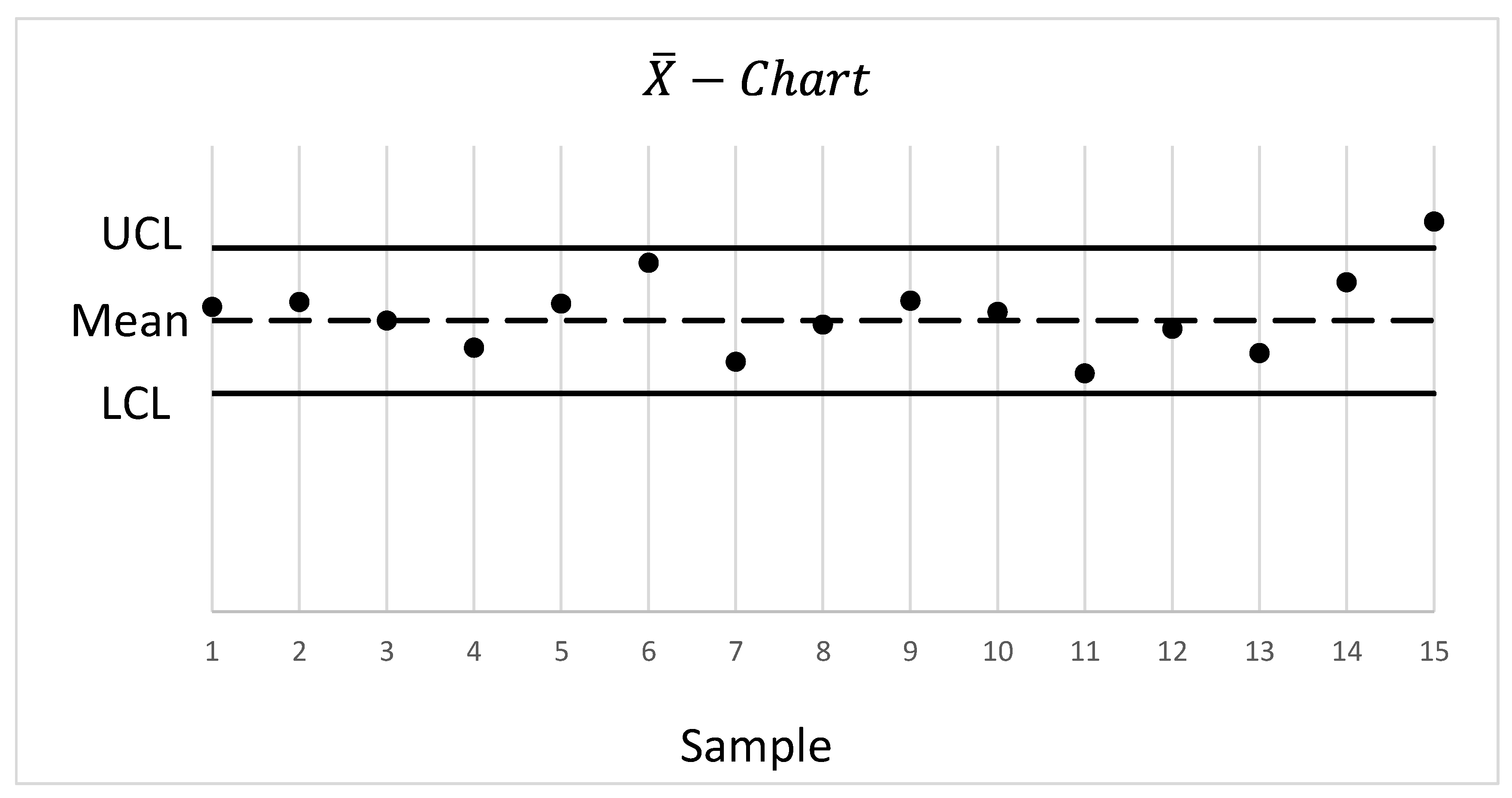
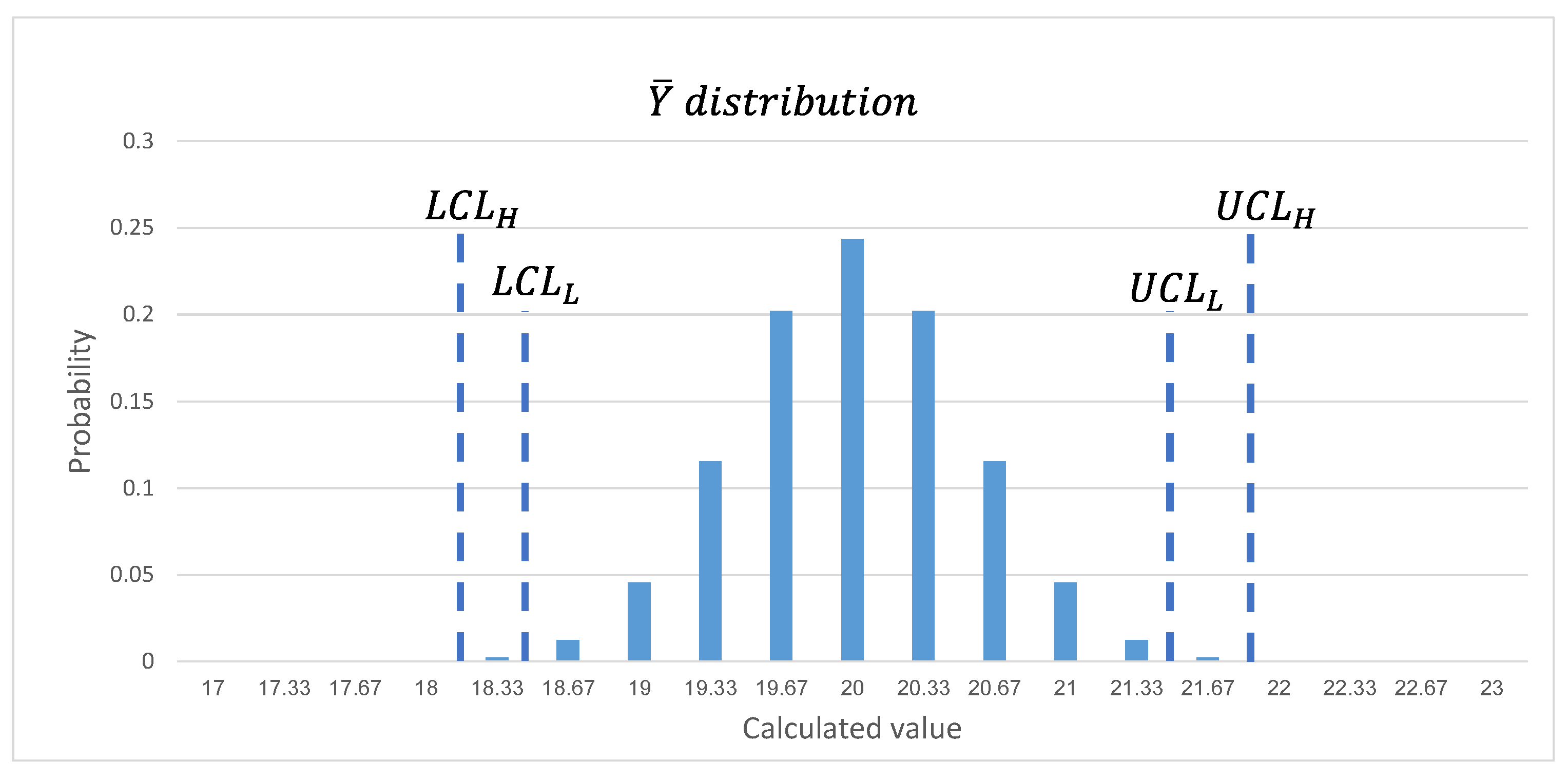
- Control limits–The -charts are set to have upper and lower control limits. These limits were constructed symmetrically around the mean as depicted in Equation (2)
5. Measurement Distribution
5.1. Symmetrical Process
5.2. Asymmetrical Process
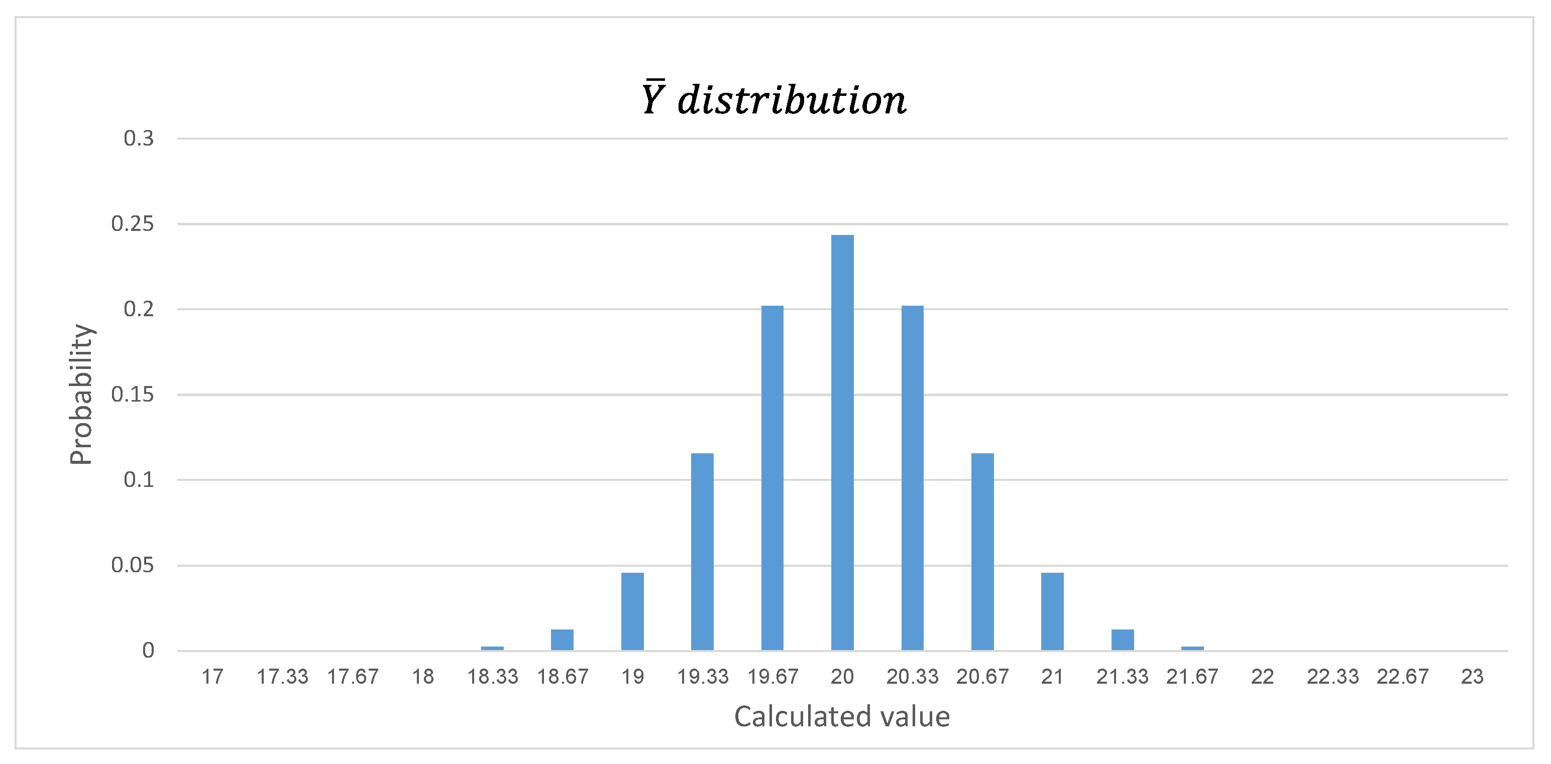
5.3. Average Sample Value Distribution
6. Asymmetry Considerations When Setting Control Limits
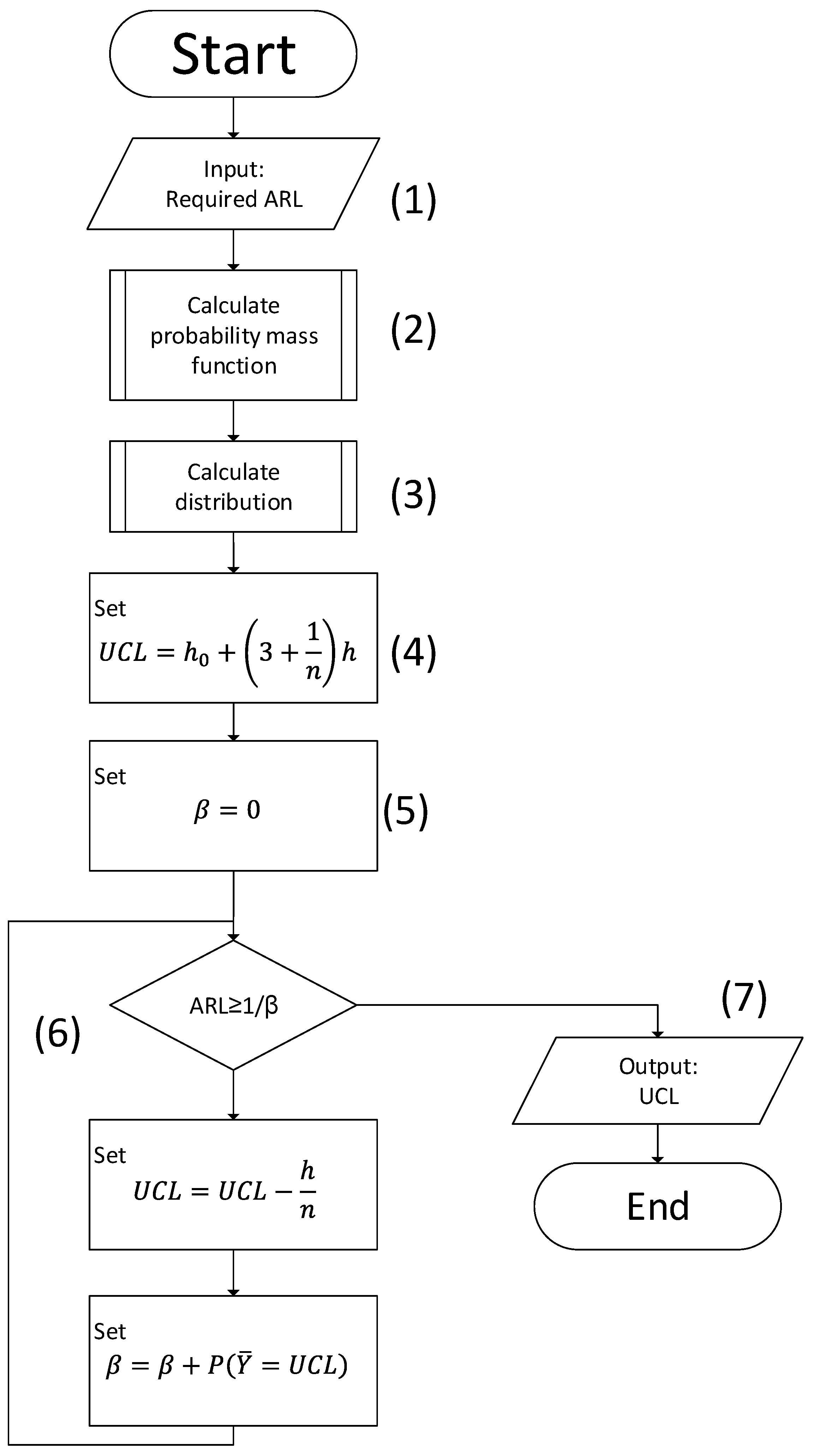
7. Suggested Method for Setting Control Limits
- (1)
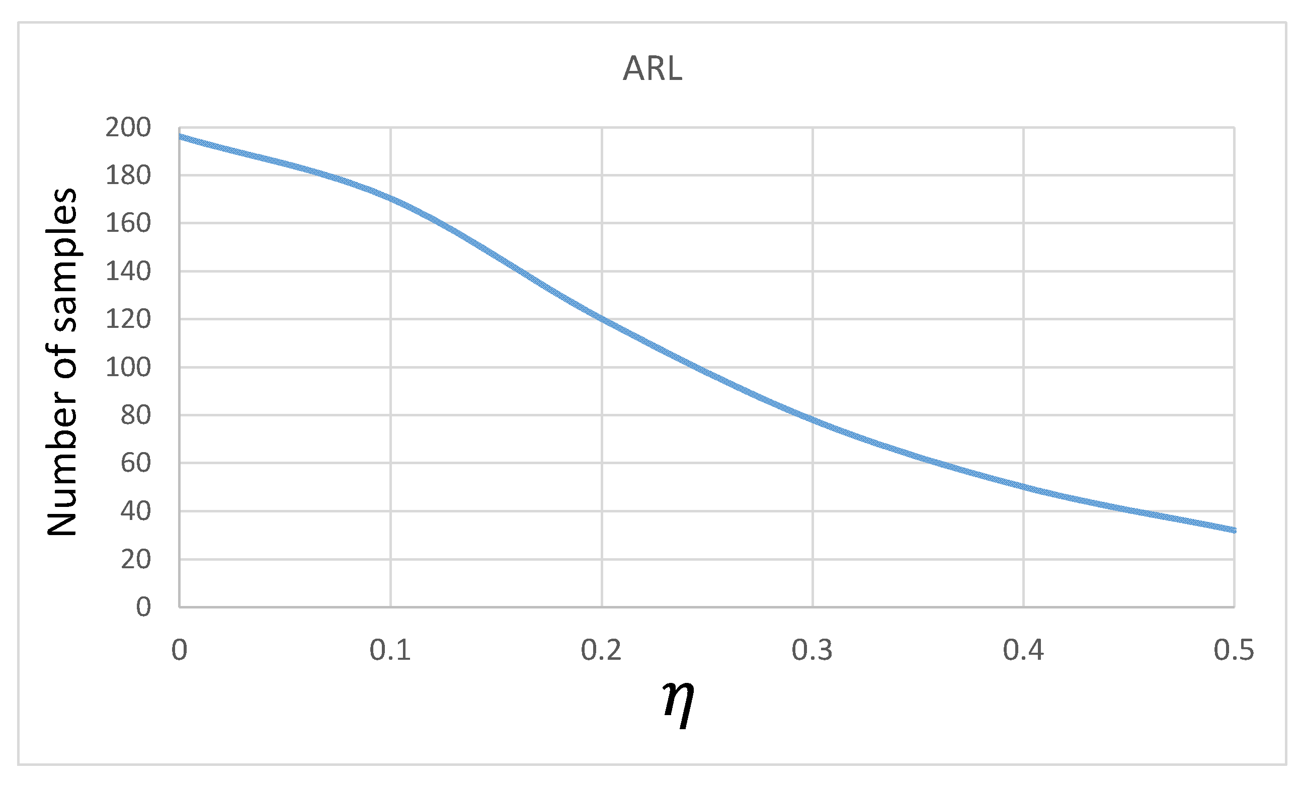
- The input for the algorithm is the required ARL {typically the same ARL is required for both upper and lower control limits, but this need not be the general case}
- (2)
- As depicted in Figure 4, the specific probability mass function for the measured value is calculated.
- (3)
- Depending on the sample size (), the values of the probability mass function’s values for are calculated.
- (4)
- is set for the initial highest possible value { is set to the initial lowest possible value, i.e., }.
- (5)
- The value of (false-alarm probability) is initialized to 0 (indicating ).
- (6)
- At each iteration, the value of the is reduced by one “notch” (reduced to the next possible measurable value of {the value of is increased by the same value}, the new is calculated, until the required is reached (i.e., the loop ends when ).
- (7)
- The calculated {} is the required output.
8. Conclusions, Limitations, and Future Research
Funding
Data Availability Statement
Conflicts of Interest
Appendix A. An Example of an Asymmetric Low-Resolution Process Control

Appendix B. Calculating the Control Limits

References
- Braden, P.; Matis, T.; Benneyan, J.T.; Chen, B. Estimating X Statistical Control Limits for Any Arbitrary Probability Distribution Using Re-Expressed Truncated Cumulants. Mathematics 2022, 10, 1044. [Google Scholar] [CrossRef]
- Bradford, P.G.; Miranti, P.J. Information in an industrial culture: Walter A. Shewhart and the evolution of the control chart, 1917–1954. Inf. Cult. 2019, 54, 179–219. [Google Scholar] [CrossRef]
- Montgomery, D.C. Introduction to Statistical Quality Control, 7th ed.; Wiley: New York, NY, USA, 2019. [Google Scholar]
- Haridy, S.; Maged, A.; Alherimi, N.; Shamsuzzaman, M.; Al-Ali, S. Optimization design of control charts: A systematic review. Qual. Reliab. Eng. Int. 2024, 40, 2122–2157. [Google Scholar] [CrossRef]
- Quintero-Arteaga, C.; Peñabaena-Niebles, R.; Vélez, J.I.; Jubiz-Diaz, M. Statistical design of an adaptive synthetic X control chart for autocorrelated processes. Qual. Reliab. Eng. Int. 2022, 28, 2475–2500. [Google Scholar] [CrossRef]
- Vardeman, S.B.; Lee, C.S. Likelihood-based statistical estimation from quantized data. Trans. Instrum. Meas. 2005, 54, 409–414. [Google Scholar] [CrossRef]
- Vardeman, S.; Hamada, M.S.; Burr, T.; Morris, M.; Wendelberger, J.; Jobe, J.M.; Moore, L.; Wu, H. An Introduction to Statistical Issues and Methods in Metrology for Physical Science and Engineering. J. Qual. Technol. 2014, 46, 33–62. [Google Scholar] [CrossRef]
- Burr, T.; Croft, S.; Vardeman, S.; Hamada, M.S.; Weaver, B. Rounding error effects in the presence of underlying measurement error. Accredit. Qual. Assur. 2012, 17, 485–490. [Google Scholar] [CrossRef]
- Lee, C.S.; Vardeman, S.B. Interval estimation of a normal process mean from rounded data. J. Qual. Technol. 2001, 33, 335–348. [Google Scholar] [CrossRef]
- Kalsoom, T.; Ramzan, N.; Ahmed, S.; Ur-Rehman, M. Advances in Sensor Technologies in the Era of Smart Factory and Industry 4.0. Sensors 2020, 20, 6783. [Google Scholar] [CrossRef]
- Schütze, A.; Helwig, N.; Schneider, T. Sensors 4.0–smart sensors and measurement technology enable Industry 4.0. J. Sens. Sens. Syst. 2018, 7, 359–371. [Google Scholar] [CrossRef]
- Gaddam, A.; Wilkin, T.; Angelova, M.; Gaddam, J.; Faults, D.S. Anomalies and Outliers in the Internet of Things: A Survey on the Challenges and Solutions. Electronics 2020, 9, 511. [Google Scholar] [CrossRef]
- Arab, M.; Akbarian, H.; Gheibi, M.; Akrami, M.; Fathollahi-Fard, A.M.; Hajiaghaei-Keshteli, M.; Tian, G. A soft-sensor for sustainable operation of coagulation and flocculation units. Eng. Appl. Artif. Intell. 2022, 115, 105315. [Google Scholar] [CrossRef]
- Zhang, C.; Fathollahi-Fard, M.A.; Li, J.; Tian, G.; Zhang, T. Disassembly Sequence Planning for Intelligent Manufacturing Using Social Engineering Optimizer. Symmetry 2021, 13, 663. [Google Scholar] [CrossRef]
- Wang, W.; Zhou, X.; Tian, G.; Fathollahi-Fard, M.A.; Wu, P.; Zhang, C.; Liu, C.; Li, Z. Multi-objective low-carbon hybrid flow shop scheduling via an improved teaching-learning-based optimization algorithm. Sci. Iran. 2022. [Google Scholar] [CrossRef]
- Pasha, J.; Dulebenets, A.M.; Fathollahi-Fard, M.A.; Tian, G.; Lau, Y.-Y.; Singh, P.; Liang, B. An integrated optimization method for tactical-level planning in liner shipping with heterogeneous ship fleet and environmental considerations. Adv. Eng. Inform. 2021, 48, 101299. [Google Scholar] [CrossRef]
- Zhao, N.; Bai, Z. Bayesian statistical inference based on rounded data. Commun. Stat. Simul. Comput. 2020, 49, 135–146. [Google Scholar] [CrossRef]
- Zhao, N.; Bai, Z. Analysis of rounded data in measurement error regression. J. Korean Stat. Soc. 2013, 42, 415–429. [Google Scholar] [CrossRef]
- Zhidong, B.; Shurong, Z.; Bauxue, Z.; Gourong, H. Statistical analysis for rounded data. J. Stat. Plan. Inference 2009, 139, 2526–2542. [Google Scholar]
- Gertsbakh, I. Measurement Theory for Engineers; Springer: Berlin, Germany, 2003. [Google Scholar]
- Sheppard, W.F. On the Calculation of the most Probable Values of Frequency-Constants, for Data arranged according to Equidistant Division of a Scale. Proc. Lond. Math. Soc. 1897, 1, 353–380. [Google Scholar] [CrossRef]
- Cochran, W.G.; Cox, G.M. Experimental Designs, 2nd ed.; John Wiley & Sons: New York, NY, USA, 1957. [Google Scholar]
- Dempster, A.P.; Rubin, D.B. Rounding error in regression: The appropriateness of Sheppard’s corrections. J. R. Stat. Soc. Ser. B (Methodol.) 1983, 45, 51–59. [Google Scholar] [CrossRef]
- Heitjan, D.F.; Rubin, D.B. Ignorability and coarse data. Ann. Stat. 1991, 19, 2244–2253. [Google Scholar] [CrossRef]
- Heitjan, D.F. Ignorability and coarse data: Some biomedical examples. Biometrics 1993, 49, 1099–1109. [Google Scholar] [CrossRef] [PubMed]
- Steiner, S.H.; Geyer, P.L.; Wesolowsky, G.O. Shewhart control charts to detect mean and standard deviation shifts based on grouped data. Qual. Reliab. Eng. Int. 1996, 12, 345–353. [Google Scholar] [CrossRef]
- Tricker, A.; Coates, E.; Okell, E. Precision of measurement and its effect on the R chart. Total Qual. Manag. 1997, 8, 296. [Google Scholar] [CrossRef]
- Bryce, R.; Gaudard, M.A.; Joiner, B.L. Estimating the standard deviation for individuals control charts. Qual. Eng. 1997, 10, 331–341. [Google Scholar] [CrossRef]
- Tricker, A.; Coates, E.; Okell, E. The effect on the R chart of precision of measurement. J. Qual. Technol. 1998, 30, 232–239. [Google Scholar] [CrossRef]
- McNames, J.; Evans, W.; Abercrombie, D. Quantization Compensation for SPC Q Charts. 2001. Available online: https://scholar.google.com/citations?view_op=view_citation&hl=zh-CN&user=IYJ5qH0AAAAJ&cstart=200&pagesize=100&sortby=pubdate&citation_for_view=IYJ5qH0AAAAJ:J-pR_7NvFogC (accessed on 16 May 2024).
- Schneeweiss, H.; Komlos, J.; Ahmad, A.S. Symmetric and asymmetric rounding: A review and some new results. AStA Adv. Stat. Anal. 2010, 94, 247–271. [Google Scholar] [CrossRef]
- Meneces, N.; Olivera, S.A.; Saccone, C.D.; Tessore, J. Effect of resolution of measurements in the behavior of exponentially weighted moving average control charts. PDA J. Pharm. Sci. Technol. 2013, 67, 288–295. [Google Scholar] [CrossRef]
- Schader, M.; Schmid, F. Small sample properties of the maximum likelihood estimators of the parameters μ and σ from a grouped sample of a normal population. Commun. Stat. -Simul. Comput. 1988, 17, 229–239. [Google Scholar] [CrossRef]
- Benson-Karhi, D.; Ellite, D.; Regev, I.; Schechtman, E. Estimation of a Normal Process Variance from Measurements with Large Round-Off Errors. IET Sci. Meas. Technol. 2013, 7, 80–189. [Google Scholar]
- Lee, C.S.; Vardeman, S.B. Interval estimation of a normal process standard deviation from rounded data. Commun. Stat.-Simul. Comput. 2002, 31, 13–34. [Google Scholar] [CrossRef]
- Carroll, R.J.; Ruppert, D.; Stefanski, L.A.; Crainiceanu, C.M. Measurement Error in Nonlinear Models: A Modern Perspective; Chapman & Hall: London, UK, 2006. [Google Scholar]
- Lee, C.S.; Vardeman, S.B. Confidence intervals based on rounded data from the balanced one-way normal random effects model. Commun. Stat. Simul. Comput. 2003, 32, 835–856. [Google Scholar] [CrossRef]
- Benson-Karhi, D.; Ellite, D.; Regev, I.; Schechtman, E. Using Measurements with Large Round-Off Errors Interval Estimation of Normal Process Variance. IET Sci. Meas. Technol. 2015, 9, 1050–1056. [Google Scholar]
- Box, G.E.; Luceno, A.; del Carmen Paniagua-Quinones, M. Statistical Control by Monitoring and Adjustment; John Wiley & Sons: New York, NY, USA, 2011. [Google Scholar]
- Shewhart, W.A. Economic Control of Quality of Manufactured Products; Macmillan And Co., Ltd.: London, UK, 1931. [Google Scholar]
- Koutras, M.V.; Bersimis, S.; Maravelakis, P.E. Statistical process control using Shewhart control charts with supplementary runs rules. Methodol. Comput. Appl. Probab. 2007, 9, 207–224. [Google Scholar] [CrossRef]
- Goedhart, R.; Schoonhoven, M.; Does, R.J. Guaranteed in-control performance for the Shewhart X and X control charts. J. Qual. Technol. 2017, 49, 155–171. [Google Scholar] [CrossRef]
- Saleh, N.A.; Mahmoud, A.M.; Keefe, M.J.; Woodall, W.H. The Difficulty in Designing Shewhart X and X Control Charts with Estimated Parameters. J. Qual. Technol. 2015, 47, 127–138. [Google Scholar] [CrossRef]
- Jensen, W.A.; Jones-Farmer, L.A.; Champ, C.W.; Woodall, W.H. Effects of parameter estimation on control chart properties: A literature review. J. Qual. Technol. 2006, 38, 349–364. [Google Scholar] [CrossRef]
- Zhou, M. Variable sample size and variable sampling interval Shewhart control chart with estimated parameters. Oper. Res. 2017, 17, 17–37. [Google Scholar] [CrossRef]
- Faraz, A.; Saniga, E.; Montgomery, D. Percentile-based control chart design with an application to Shewhart and S2 control charts. Qual. Reliab. Eng. Int. 2019, 35, 116–126. [Google Scholar] [CrossRef]
- Das, T. Control chart for continuous quality improvement-analysis in the industries of Bangladesh. Mil. Inst. Sci. Technol. 2017, 5, 65–72. [Google Scholar]
- Jardim, F.; Chakraborti, S.; Epprecht, E.K. Two perspectives for designing a phase II control chart with estimated parameters: The case of the Shewhart Chart. J. Qual. Technol. 2020, 52, 198–217. [Google Scholar] [CrossRef]
- Al-Omari, A.I.; Haq, A. Improved quality control charts for monitoring the process mean, using double-ranked set sampling methods. J. Appl. Stat. 2012, 39, 745–763. [Google Scholar] [CrossRef]
- Dalalah, D.; Diabat, A. Repeatability and reproducibility in med labs: A procedure to measurement system analysis. IET Sci. Meas. Technol. 2015, 9, 826–835. [Google Scholar] [CrossRef]
- Khakifirooz, M.; Tercero-Gómez, V.G.; Woodallb, W.H. The role of the normal distribution in statistical process monitoring. Qual. Eng. 2021, 33, 497–510. [Google Scholar] [CrossRef]


| Notation | Explanation |
|---|---|
| Process parameters | |
| Real value of the measured controlled parameter. This value is unknown and cannot be measured and approximated by the measured value | |
| Real average value of the obtained sample. This value is unknown and estimated by | |
| Mean value of the controlled process value | |
| Standard deviation of the controlled process real value. It is assumed that the process values are normally distributed. | |
| Measurement parameters | |
| Resolution of the measuring device. For example: a thermometer that can only measure in units of °C | |
| Measured value of the controlled process. | |
| Measured average value of the controlled process. | |
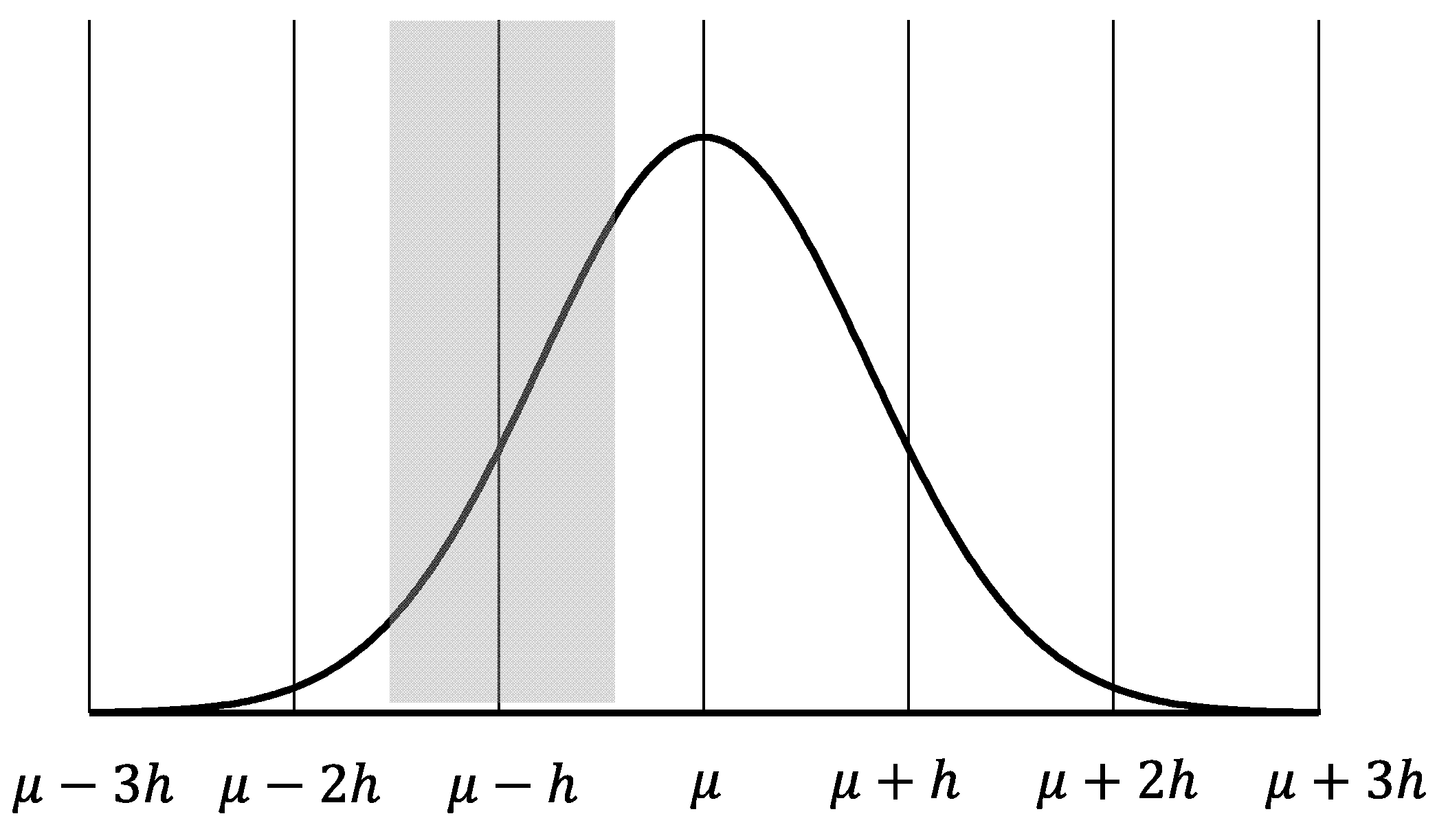
| Asymmetry measure. The minimal distance between the process’s mean, the closest measurable value | |
| Ratio between the standard deviation of the controlled process and the measuring resolution (). | |
| Average run length—the average number of samples until a deviation of the process from the designed mean is discovered. | |
| Sample size from the controlled process. | |
| Decision variables | |
| Lower and upper control limits of the controlled process | |
| General notation | |
| Normal distribution cumulative function | |
| Measured Value | Probability | |||||||
|---|---|---|---|---|---|---|---|---|
| 17 | 18 | 19 | 20 | 21 | 22 | 23 | ||
| 0 | 0 | 0 | 0 | 0 | 0 | 3 | ||
| 0 | 0 | 0 | 0 | 0 | 1 | 2 | ||
| ….. | ||||||||
| 3 | 0 | 0 | 0 | 0 | 0 | 0 | ||
Disclaimer/Publisher’s Note: The statements, opinions and data contained in all publications are solely those of the individual author(s) and contributor(s) and not of MDPI and/or the editor(s). MDPI and/or the editor(s) disclaim responsibility for any injury to people or property resulting from any ideas, methods, instructions or products referred to in the content. |
© 2024 by the author. Licensee MDPI, Basel, Switzerland. This article is an open access article distributed under the terms and conditions of the Creative Commons Attribution (CC BY) license (https://creativecommons.org/licenses/by/4.0/).
Share and Cite
Etgar, R. Asymmetry Considerations in Constructing Control Charts: When Symmetry Is Not the Norm. Symmetry 2024, 16, 811. https://doi.org/10.3390/sym16070811
Etgar R. Asymmetry Considerations in Constructing Control Charts: When Symmetry Is Not the Norm. Symmetry. 2024; 16(7):811. https://doi.org/10.3390/sym16070811
Chicago/Turabian StyleEtgar, Ran. 2024. "Asymmetry Considerations in Constructing Control Charts: When Symmetry Is Not the Norm" Symmetry 16, no. 7: 811. https://doi.org/10.3390/sym16070811
APA StyleEtgar, R. (2024). Asymmetry Considerations in Constructing Control Charts: When Symmetry Is Not the Norm. Symmetry, 16(7), 811. https://doi.org/10.3390/sym16070811