
Temperature Evaluation Considering Gradient Distribution for MV Cable XLPE Insulation Based on Wave Velocity

Abstract
:1. Introduction
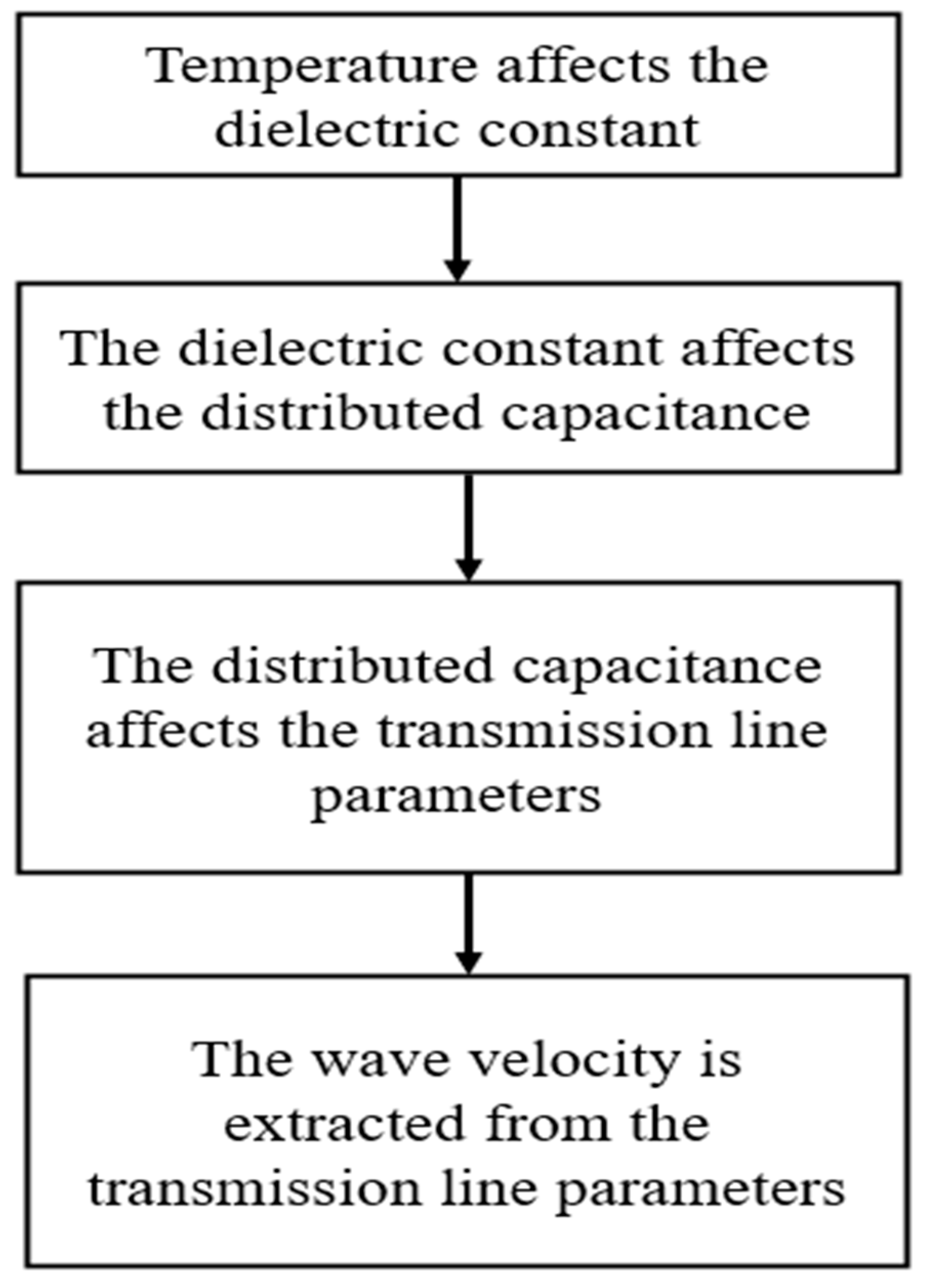
2. Methodology
3. Computational Analysis
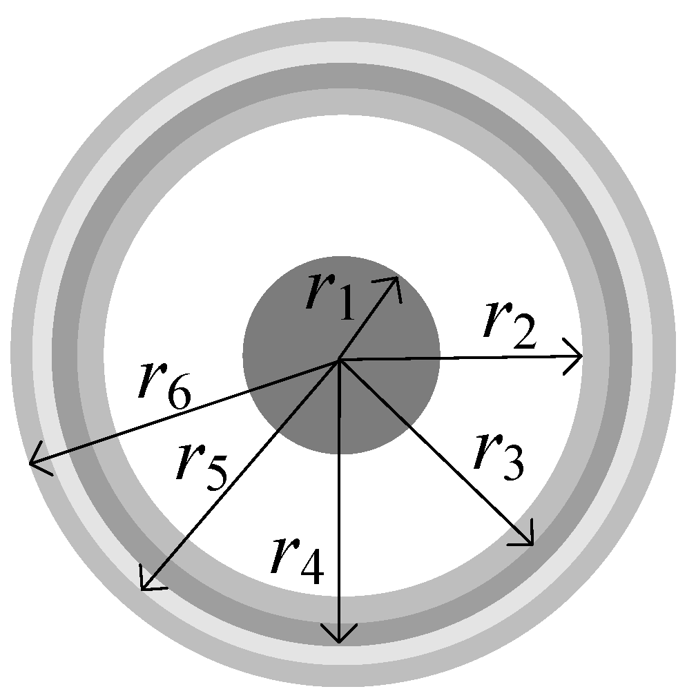
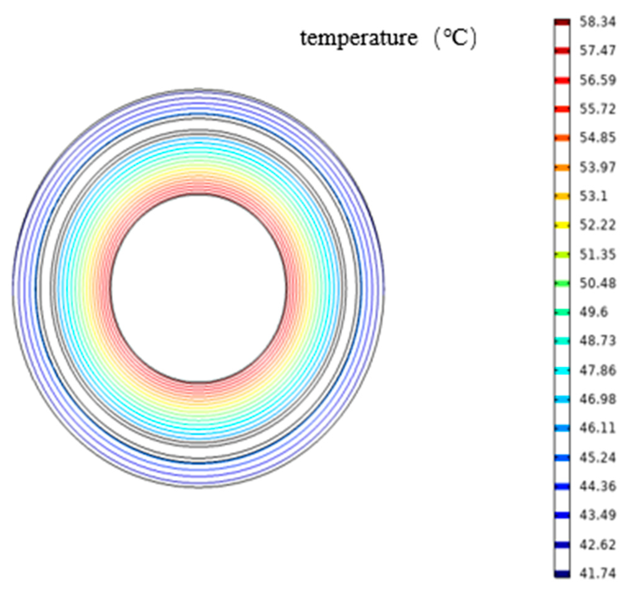
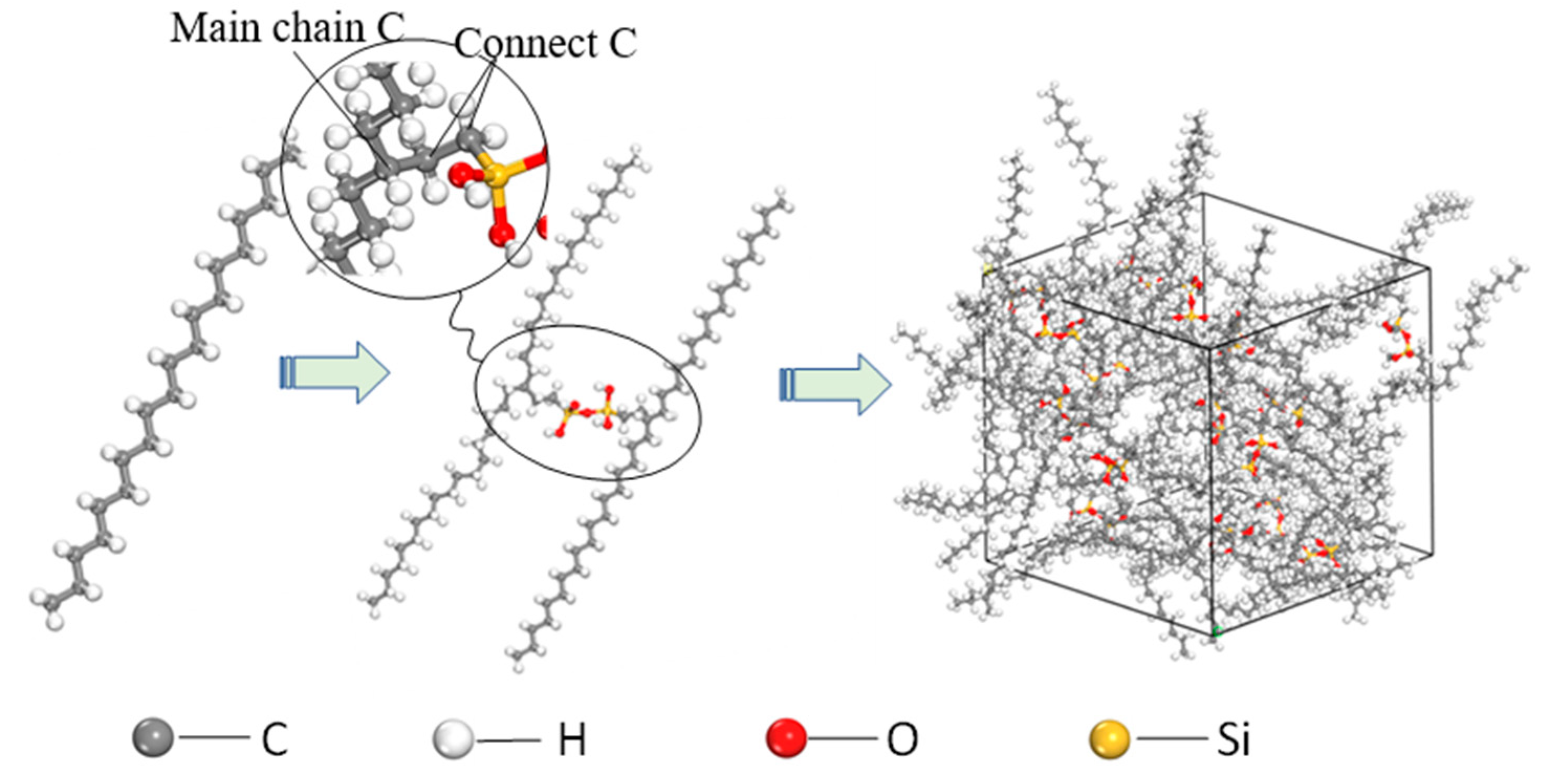
3.1. Model Establishement
3.2. Simulation Process
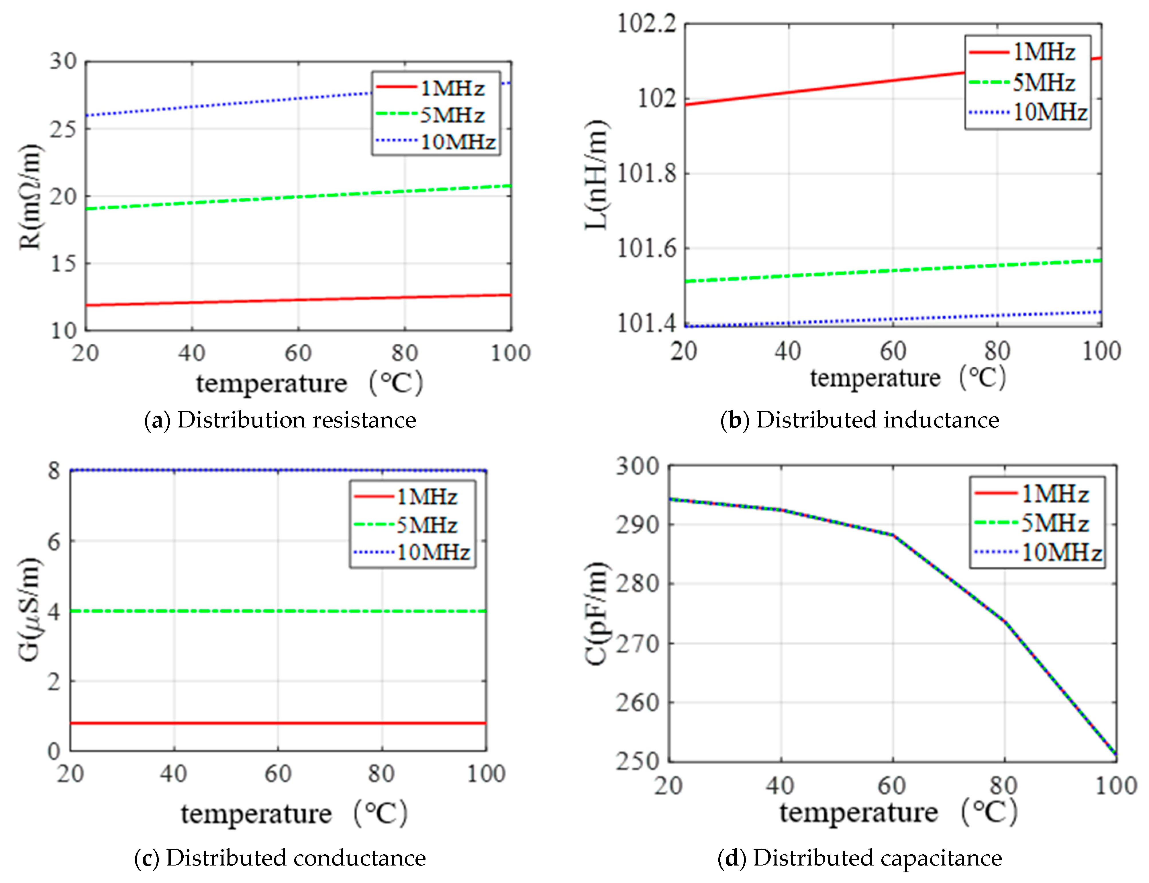
3.3. Analysis of Results
4. Analysis of Results
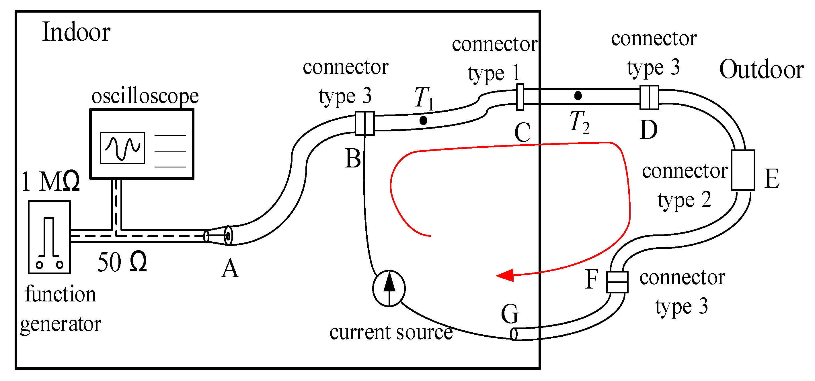
4.1. Cable Insulation Temperature Measurement Experiment
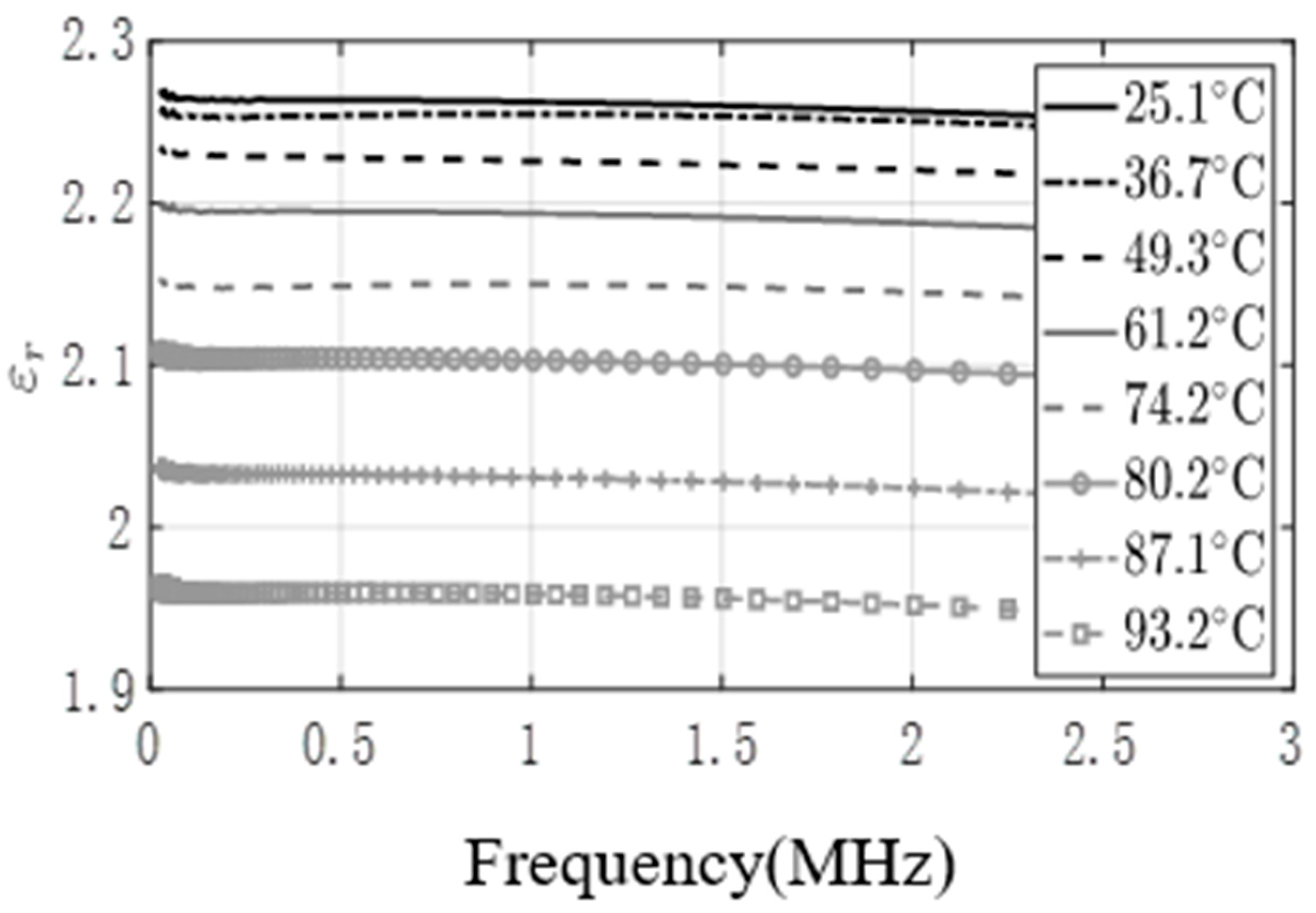
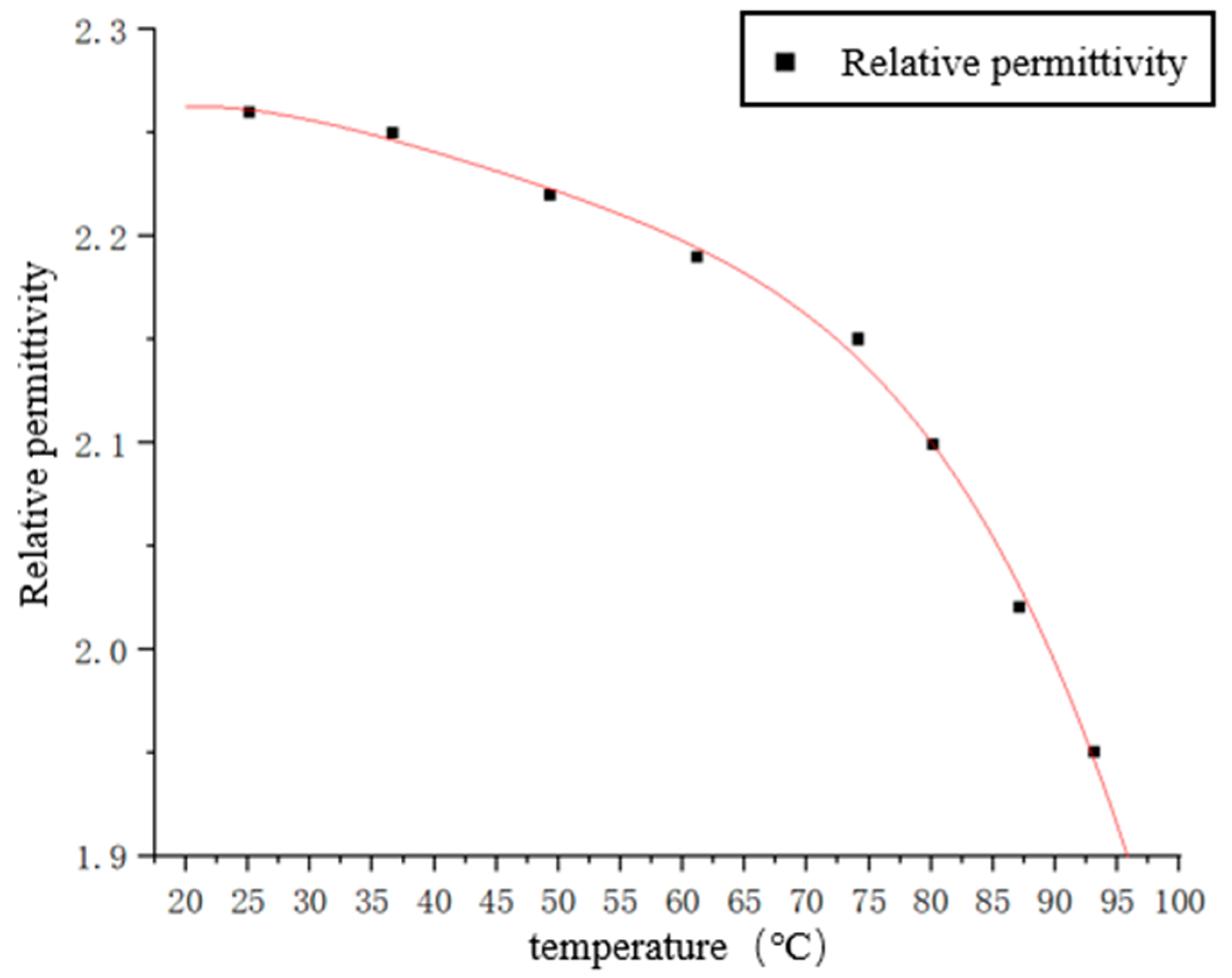
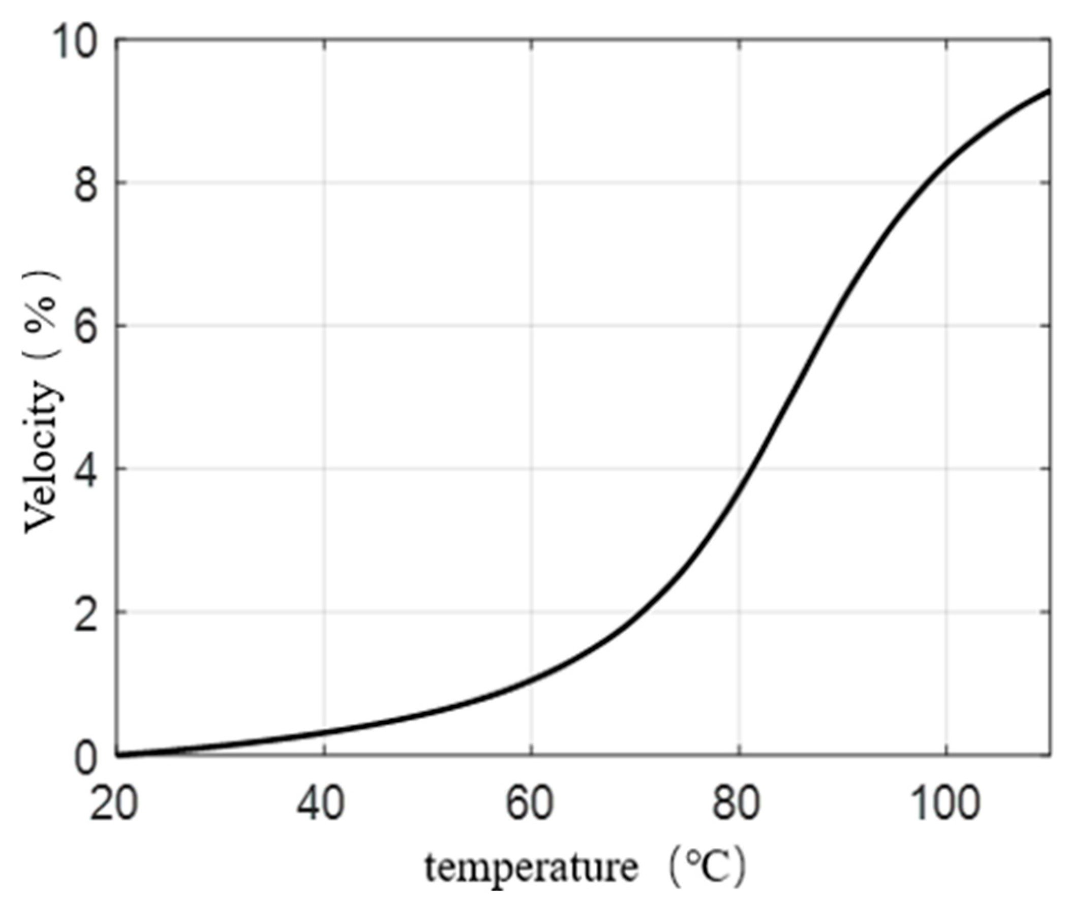
4.2. Discussion of Temperature Effect on Dielectric Constant of Cable Insulation Material


5. Conclusions
Author Contributions
Funding
Data Availability Statement
Conflicts of Interest
References
- Song, Y.; Chen, W.; Wan, F.; Zhang, Z.; Du, L.; Wang, P.; Li, J.; Wu, Z.; Huang, H. Online Multi-parameter Sensing and Condition Assessment Technology for Power Cables: A review. Electr. Power Syst. Res. 2022, 210, 108140. [Google Scholar] [CrossRef]
- Qin, T.; Mao, H.; Geng, F.; Shang, J.; Huang, Y.; Qin, C. Influence of Cable Fire Protection Measures on Current Carrying Capacity. In Proceedings of the Power System and Green Energy Conference (PSGEC), Shanghai, China, 25–27 August 2022; IEEE: Piscataway, NJ, USA, 2022; pp. 1165–1169. [Google Scholar]
- Lewandowski, R.; Banaszak, S. Shrinkback Phenomenon in High-Temperature Medium-Voltage Cables With Fluorinated Ethylene Propylene Insulation. IEEE Trans. Dielectr. Electr. Insul. 2024, 31, 1603–1610. [Google Scholar] [CrossRef]
- Alam, M.R.; Nguyen, P.T.H.; Naranpanawe, L.; Saha, T.K.; Lankeshwara, G. Allocation of Dynamic Operating Envelopes in Distribution Networks: Technical and Equitable Perspectives. IEEE Trans. Sustain. Energy 2023, 15, 173–186. [Google Scholar] [CrossRef]
- Oktay, A.; Cihat, C.U.; Celal, F.K. Insulation Evaluation of MV Underground Cable with Partial Discharge and Dielectric Dissipation Factor Measurements. Electr. Power Syst. Res. 2023, 220, 109338. [Google Scholar]
- Chen, Y.; Wang, S.; Hao, Y.; Yao, K.; Li, H.; Jia, F.; Yue, D.; Shi, Q.; Cheng, Y.; Huang, X. Temperature Monitoring for 500 kV Oil-filled Submarine Cable Based on BOTDA Distributed Optical Fiber Sensing Technology: Method and Application. IEEE Trans. Instrum. Meas. 2022, 71, 1–10. [Google Scholar] [CrossRef]
- Bragatto, T.; Cresta, M.; Gatta, F.M.; Geri, A.; Maccioni, M.; Paulucci, M. Assessing Thermal Behavior of Medium Voltage Cable Joints Through Simulations and Measurements. IEEE Trans. Ind. Appl. 2023, 59, 5705–5714. [Google Scholar] [CrossRef]
- Qi, B.; Qin, C.; Shang, H. Simulation of LXPE Cable Insulation On-line Monitoring Based on TM Electromagnetic Wave Spectrum Characteristics. Acta Microsc. 2019, 28, 169. [Google Scholar]
- Zhou, Z.; Zhang, D.; He, J.; Li, M. Local Degradation Diagnosis for Cable Insulation Based on Broadband Impedance Spectrosopy. IEEE Trans. Dielectr. Electr. Insul. 2015, 22, 2097–2107. [Google Scholar] [CrossRef]
- Li, C.; Chu, Z.; Zhang, L.; Zhang, J.; Tao, J. Insulation Aging Diagnosis and Defect Location of Crosslinked Polyethylene Cable in the Distribution Network Based on Radio Frequency Identification. Mater. Express 2023, 13, 1772–1781. [Google Scholar] [CrossRef]
- Shan, B.; Li, S.; Yu, L.; Wang, W.; Li, C.; Meng, X. Effect of Segmented Thermal Aging on Defect Location Accuracy in XLPE Distribution Cables. IEEE Access 2021, 9, 134753–134761. [Google Scholar] [CrossRef]
- Ohki, Y.; Hirai, N. Location Attempt of a Degraded Portion in a Long Polymer-insulated Cable. IEEE Trans. Dielectr. Electr. Insul. 2018, 25, 2461–2466. [Google Scholar] [CrossRef]
- Xie, Y.; Zhao, Y.; Liu, G.; Huang, J.; Li, L. Annealing Effects on XLPE Insulation of Retired High-voltage Cable. IEEE Access 2019, 7, 104344–104353. [Google Scholar] [CrossRef]
- Dubickas, V.; Edin, H. On-line Time Domain Reflectometry Measurements of Temperature Variations of an XLPE Power Cable. In Proceedings of the IEEE Conference on Electrical Insulation and Dielectric Phenomena, Kansas City, MO, USA, 15–18 October 2006. [Google Scholar]
- Nyamupangedengu, C.; Sotsaka, M.; Mlangeni, G.; Ndlovu, L.; Munilal, S. Effect of Temperature Variations on Wave Propagation Characteristics in Power Cables. SAIEE Afr. Res. J. 2015, 106, 28–38. [Google Scholar] [CrossRef]
- de Clippelaar, S.; Kruizinga, B.; van der Wielen, P.C.; Wouters, P.A. Wave-Velocity Based Real-Time Thermal Monitoring of Medium-Voltage Underground Power Cables. IEEE Trans. Power Deliv. 2024, 39, 983–991. [Google Scholar] [CrossRef]
- Liang, R.; Zhang, Z.; Li, H.; Chi, P.; Li, G.; Tao, Y. Partial Discharge Location of Power Cables Based on an Improved Single-terminal Method. Electr. Power Syst. Res. 2021, 193, 107013. [Google Scholar] [CrossRef]
- Paul, C.R. Decoupling the Multiconductor Transmission Line Equations. IEEE Trans. Microw. Theory Tech. 1996, 44, 1429–1440. [Google Scholar] [CrossRef]
- Li, Y.; Wouters, P.A.A.F.; Wagenaars, P.; van der Wielen, P.C.J.M.; Steennis, E.F. Estimation of Transmission Line Parameters Single-core XLPE Cables Considering Semiconducting Layer. In Proceedings of the IEEE International Conference on Condition Monitoring and Diagnosis, Bali, Indonesia, 23–27 September 2012. [Google Scholar]
- Ander, G.J. Rating of Electric Power Cables in Unfavorable Thermal Environment, 1st ed.; IEEE Press Series on Power Engineering; Wiley: Hoboken, NJ, USA, 2005; Volume 23, pp. 1–73. [Google Scholar]
- He, X.; Zhang, S.; Zhou, Y.; Zheng, F.; Lu, Q. The Fluorine Impact on Dielectric Constant of Polyimides: A Molecular Simulation Study. Polymer 2022, 254, 125073. [Google Scholar] [CrossRef]
- Stalter, S.; Yelash, L.; Emamy, N.; Statt, A.; Hanke, M.; Lukáčová-Medvid’ová, M.; Virnau, P. Molecular Dynamics Simulations in Hybrid Particle-continuum Schemes: Pitfalls and Caveats. Comput. Phys. Commun. 2018, 224, 198–208. [Google Scholar] [CrossRef]
- Yin, F.; Yang, L.; Mo, Y.; Hou, W.; Yuan, Y. Origin of Low Dielectric Permittivity in Crosslinked Cellulose/Kevlar Fiber Composites as Revealed Via Molecular Dynamics Simulation. Mater. Chem. Phys. 2022, 286, 126008. [Google Scholar] [CrossRef]
- Hou, W.; Yang, L.; Mo, Y.; Yin, F.; Huang, Y.; Zheng, X. Static Dielectric Constant and Dielectric Loss of Cellulose Insulation: Molecular dynamics simulations. High Volt. 2021, 6, 1051–1060. [Google Scholar] [CrossRef]
- Wei, Y.; Yang, J.; Li, G.; Zhou, X.; Hao, C.; Lei, Q.; Li, S. Influence of Molecular Chain Side Group on the Electrical Properties of Silicone Rubber and Mechanism Analysis. IEEE Trans. Dielectr. Electr. Insul. 2022, 29, 1465–1473. [Google Scholar] [CrossRef]


| Symbol (Unit) | Meaning | Value |
|---|---|---|
| ρc (Ωm) | Core resistivity | 2.82 × 10⁻⁸ |
| ρsi (Ωm) | Inner buffer resistivity | 0.01 |
| ρso (Ωm) | Resistivity of the outer buffer layer | 0.01 |
| ρs (Ωm) | Metal shield resistivity | 1.68 × 10⁻⁸ |
| r1 (mm) | Core radius | 9.5 |
| r2 (mm) | Radius of the insulation | 15.6 |
| r3 (mm) | Inner buffer layer radius | 16.0 |
| r4 (mm) | Metal shield radius | 17.15 |
| r5 (mm) | Radius of the outer buffer layer | 17.6 |
| r6 (mm) | Outer sheath radius | 20.1 |
| εXLPE | XLPE relative permittivity | 2.23–0.001 j |
| εcs | The relative permittivity of the inner shield | 1000 |
| εls | The relative permittivity of the outer shield | 1000 |
| εj | Dielectric constant of the outer sheath | 2.3 |
| Ri | Thermal resistance of insulation Km/W | 0.27 |
| Rb1 | Thermal resistance between insulation and shielding Km/W | 0.03 |
| Ri | Thermal resistance of insulation Km/W | 0.27 |
| Rb1 | Thermal resistance between insulation and shielding Km/W | 0.03 |
| Rb2 | Thermal resistance between shield and outer sheath Km/W | 0.02 |
| Rj | Thermal resistance of the outer sheath Km/W | 0.07 |
| Qc | Conductor heat capacity J/m/K | 694 |
| Qi | Insulation heat capacity J/m/K | 946 |
| Qb1 | The heat capacity between insulation and shield is J/m/K | 89 |
| Qs | Shielding heat capacity J/m/K | 413 |
| Parameter | Percent Change |
|---|---|
| R | 8.3% |
| L | 0.1% |
| G | −0.1% |
| C | −15% |
| Symbol | Parameters | Value |
|---|---|---|
| Wc | Conductor loss W/m | 34.5 |
| Tconductor | Conductor temperature °C | - |
| Tearthscreen | Metal shielding temperature °C | - |
| Tjacket | Epidermal temperature °C | - |
| pi, pb1, pb2, pb | Van Wormer coefficient | 0.42, 0.5, 0.5, 0.48 |
| Tj °C | Ti °C | Tiv °C |
|---|---|---|
| 20.4 | 33.7 | 32 |
| 28.6 | 42.0 | 44 |
| 37.3 | 50.7 | 49 |
| 48.7 | 62.1 | 61 |
Disclaimer/Publisher’s Note: The statements, opinions and data contained in all publications are solely those of the individual author(s) and contributor(s) and not of MDPI and/or the editor(s). MDPI and/or the editor(s) disclaim responsibility for any injury to people or property resulting from any ideas, methods, instructions or products referred to in the content. |
© 2024 by the authors. Licensee MDPI, Basel, Switzerland. This article is an open access article distributed under the terms and conditions of the Creative Commons Attribution (CC BY) license (https://creativecommons.org/licenses/by/4.0/).
Share and Cite
Liu, Y.; Liu, J.; Zhang, L.; Liang, Y.; Zhong, Y.; Li, Y. Temperature Evaluation Considering Gradient Distribution for MV Cable XLPE Insulation Based on Wave Velocity. Symmetry 2024, 16, 834. https://doi.org/10.3390/sym16070834
Liu Y, Liu J, Zhang L, Liang Y, Zhong Y, Li Y. Temperature Evaluation Considering Gradient Distribution for MV Cable XLPE Insulation Based on Wave Velocity. Symmetry. 2024; 16(7):834. https://doi.org/10.3390/sym16070834
Chicago/Turabian StyleLiu, Yan, Jianben Liu, Longxiang Zhang, Yuwei Liang, Yuyao Zhong, and Yan Li. 2024. "Temperature Evaluation Considering Gradient Distribution for MV Cable XLPE Insulation Based on Wave Velocity" Symmetry 16, no. 7: 834. https://doi.org/10.3390/sym16070834