Abstract
Asymmetric distributions are frequently seen in real-world datasets due to a number of factors, such as sample biases and nonlinear interactions between the variables observed. Thus, in order to better characterize real-world phenomena, studying asymmetric distribution is of great interest. In this work, we derive stress–strength reliability formulas of the type when both X and Y follow p-max stable laws with three parameters, which are inherently asymmetric. The new relations are given in terms of extreme-value H-functions and have been obtained under fewer parameter restrictions when compared to similar results in the literature. We estimate the parameters of the p-max stable laws by a stochastic optimization method and the stress–strength probability by a maximum likelihood procedure. The performance of the analytical models is evaluated through simulations and real-life dataset modeling.
1. Introduction
Reliability measures of the type , often represented as R and referred to as stress–strength reliability, are important for evaluating the performance of different systems and processes. This measure indicates the probability that a random variable X, which can represent a general performance metric or quality indicator, is less than another random variable Y, which could signify a threshold or standard to be met. In this context, X and Y are not limited to engineering concepts like stress and strength but are applicable in any scenario where two quantities are compared. A higher R value signifies a more reliable system, indicating a greater likelihood that the performance metric X will be below the threshold Y. Calculating requires an understanding of the joint distribution of X and Y, which can be determined through various methods, including simulation, analytical solutions, or the use of copulas to model dependencies between variables. We refer the reader to [1] for further details on this subject.
Let Y and X be independent continuous random variables from probability density function (PDF) and cumulative distribution function (CDF) , respectively. We can write the stress–strength reliability measure as:
Thus, R is a measure of component reliability, and it may be interpreted as the probability of a system failure when the applied stress Y is greater than its strength X. It is often assumed that X and Y are independent random variables and that they belong to the same family of probability distributions. Rathie et al. [2] present a recent survey on the subject.
Studying reliability measures such as for asymmetric marginal distributions is crucial for understanding a variety of real-world scenarios that require data-driven solutions. In the case of finance applications, where risk assessment is critical, asymmetric distributions play a central role, especially heavy tailed ones [3]. For example, in stock market analysis, knowing the likelihood that a particular stock will do better than another is crucial to making wise investment choices. Investors can efficiently manage risk and optimize their portfolios with the aid of reliability metrics, which assist in quantifying these probabilities [4].
Furthermore, asymmetry in distributions is common in a wide range of social and ecological phenomena, including the spread of illnesses and the distribution of money [5]. Asymmetric distributions can be used to describe the different scenarios of disease transmission within populations in epidemiology [6]. Researchers can better understand the likelihood of particular outcomes and aid in the creation of tailored intervention methods by examining reliability measurements in such circumstances. In short, studying reliability measures of the type for asymmetric distributions makes modeling and prediction more precise, which in turn helps one to make more informed decisions across a variety of domains.
In particular, reliability measures of the stress–strength type for classic extreme value distributions were studied by [7], who derived expressions for R in terms of special functions for l-max stable laws (Fréchet, Weibull, and Gumbel). Several authors have worked on the estimation and application of stress–strength for the l-max stable distributions (e.g., [8,9,10,11]). Some generalizations of l-max stable distributions have been proposed to either allow better data fitting or provide more convenient mathematical properties. In the work of Aryal and Tsokos [12], for example, the generalized extreme value distribution (GEV) was extended to a model named transmuted GEV (TGEV). Bivariate data were also considered like bimodal Weibull [13], bimodal Gumbel [14], and bimodal GEV (BGEV) [15] distributions.
The l-max stable distributions are derived as a limiting distribution of linearly normalized partial maxima. Another approach to generalize such distributions is by non-linearly normalizing partial maxima of independent identically distributed random variables (iid RVs). This way, for a given CDF , suppose there exists sequences of real numbers and with such that
weakly, where is a non-degenerate CDF. The three-parameter p-max stable laws can be obtained from CDF (2) by the definition of the same p-type. That means that we assume there exist positive constants such that
where for . It was shown in [16] that H is of the same p-type as one of the following distributions: log-Fréchet, log-Weibull, inverse log-Fréchet, inverse log-Weibull, standard Fréchet, and standard Weibull. Such limiting distributions are heavy tailed and asymmetric. Therefore, the convergence in (2) is usually studied by assessing the approximation on the tails, as discussed, for example, by Feng and Chen [17] and references therein.
To the best of our knowledge, the literature lacks previous in-depth studies on reliability inference for p-max stable distributions, and this work stands as a contribution by providing estimation methods for R based on stochastic optimization for this class of distributions. Thus, in this paper, we consider the problem of estimating the stress–strength parameter R when X and Y are independent three-parameter p-max stable random variables with the same CDF but different parameters. In order to validate our results, a robust framework was proposed and applied to model real and synthetic datasets, rigorously indicating the capacities of the p-max models and the usability of the analytical formulas hereby derived to calculate R.
Our main contributions are as follows:
- to analytically derive R in terms of special functions, for each three-parameter p-max stable law with fewer parameter restrictions compared to previous results in the literature;
- to propose an estimator for R;
- to apply the results to the modeling of real datasets. In particular, two real scenarios are investigated, showing the versatility of stress–strength reliability (SSR) modeling approaches using p-max models. First, soccer pass completion proportions of two different championships (UEFA Champions League and 2022 FIFA World Cup) were compared, allowing scouting professionals to use the SSR results as a proxy for technical level comparison of teams that competed at those tournaments. Then, a second application involved the modeling and comparison of the strength of carbon fibers of different lengths when subjected to tension efforts. In both modeling scenarios, the best fitting p-max stable distribution (both qualitatively (by graphical methods) and quantitatively (by information criteria)) was taken as a starting point.
This paper is organized as follows: Section 2 introduces preliminaries, especially the definition of the -function, the -function, and the three-parameter p-max stable laws. Section 3, on the other hand, deals with the derivation of R when X and Y are independent p-max stable random variables. The maximum likelihood estimation for R is presented in Section 4. In Section 5, we deal with Monte Carlo simulations as well as with the modeling of two real situations involving football datasets and different-length carbon fibers. The Section 6 deals with conclusions.
2. Preliminaries
In this section, we give some definitions and results, which will be used subsequently.
2.1. Special Functions
The -function is defined by
where , , (not both m and n simultaneously zero), (), (), and and are complex numbers such that no poles of ( coincide with poles of (. L is a suitable contour to , , separating the poles of the two types mentioned above. For more details, see [18]. As a special case, for , , and , we have
Next, let us consider the extreme-value H-function, recently defined in [19]. Thus, this function, hereby denoted as , can be defined as
where , not both and can be equal to zero at the same time, when or and , and when and . In this paper, , , and ℜ denote the real numbers, complex numbers, and the real part of a complex number, respectively.
An important special case of this function is obtained by taking , which represents an upper (or lower) bound for its value depending on the sign of . This case is, therefore, an extreme value of the function and can be written in terms of the -function as [19]:
when and
otherwise.
In the next sections, we prove that all stress–strength probabilities involving three-parameter -max stable laws can be written as -functions and, in addition, some parameter restrictions allow Equation (3) to be readily used.
2.2. Three-Parameter p-Max Stable Laws
As indicated, the three-parameter p-max stable laws are obtained by taking CDFs of the types , , where all satisfy (2) such that:
where . These distributions are called Extreme Value Distributions under power normalization or p-max stable laws, and they are known, respectively, as log-Fréchet, log-Weibull, inverse log-Fréchet, inverse log-Weibull, standard Fréchet, and standard Weibull. For a complete characterization of these distributions see [20].
The corresponding three-parameter PDFs are given by
where , and denote the indicator function of the set A.
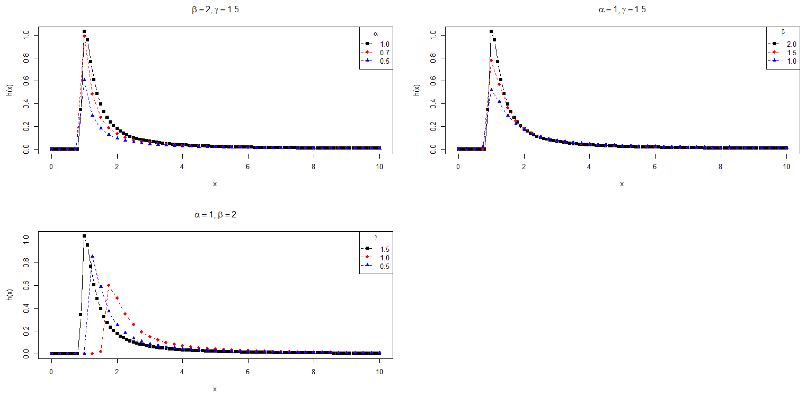
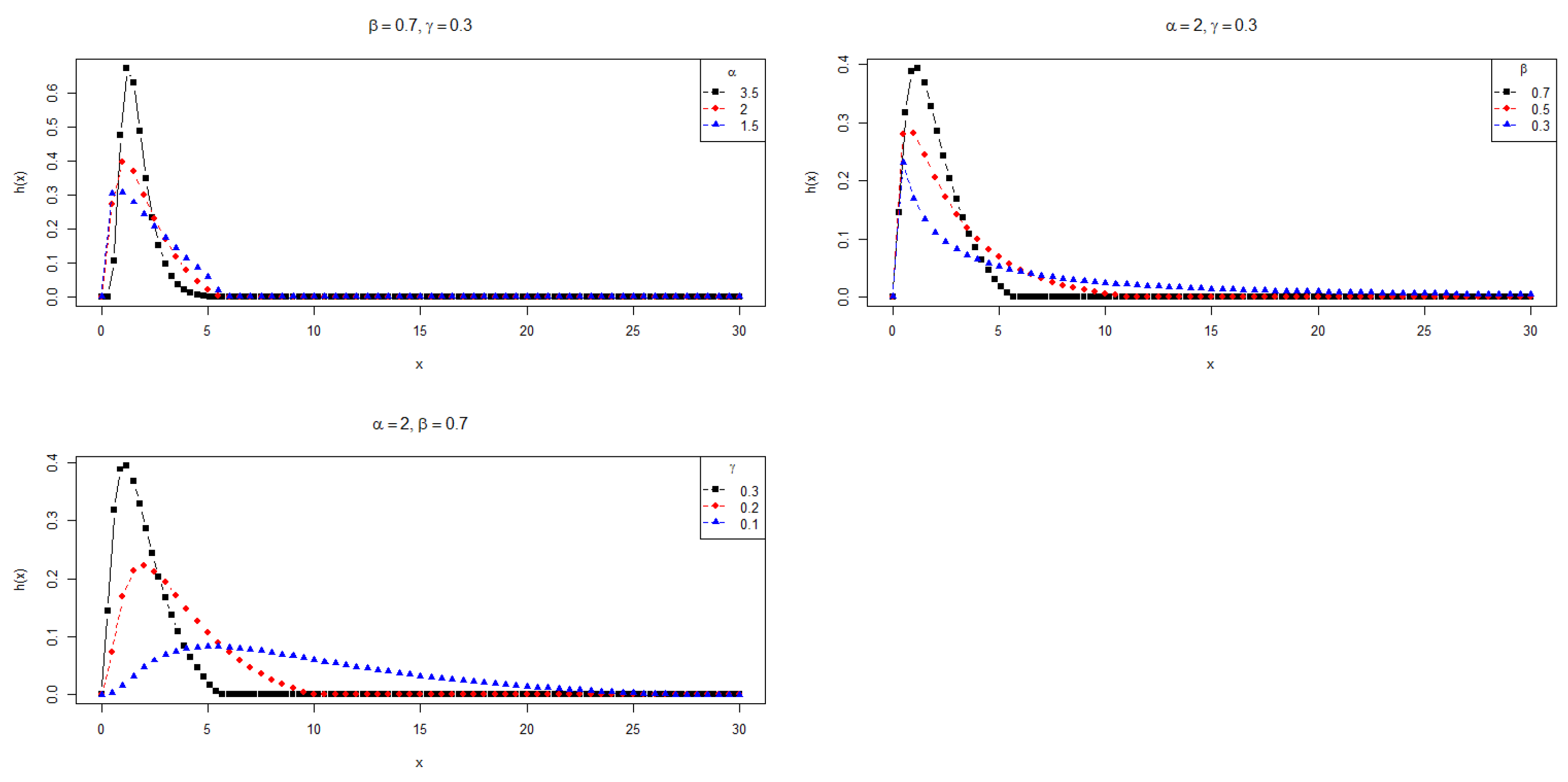
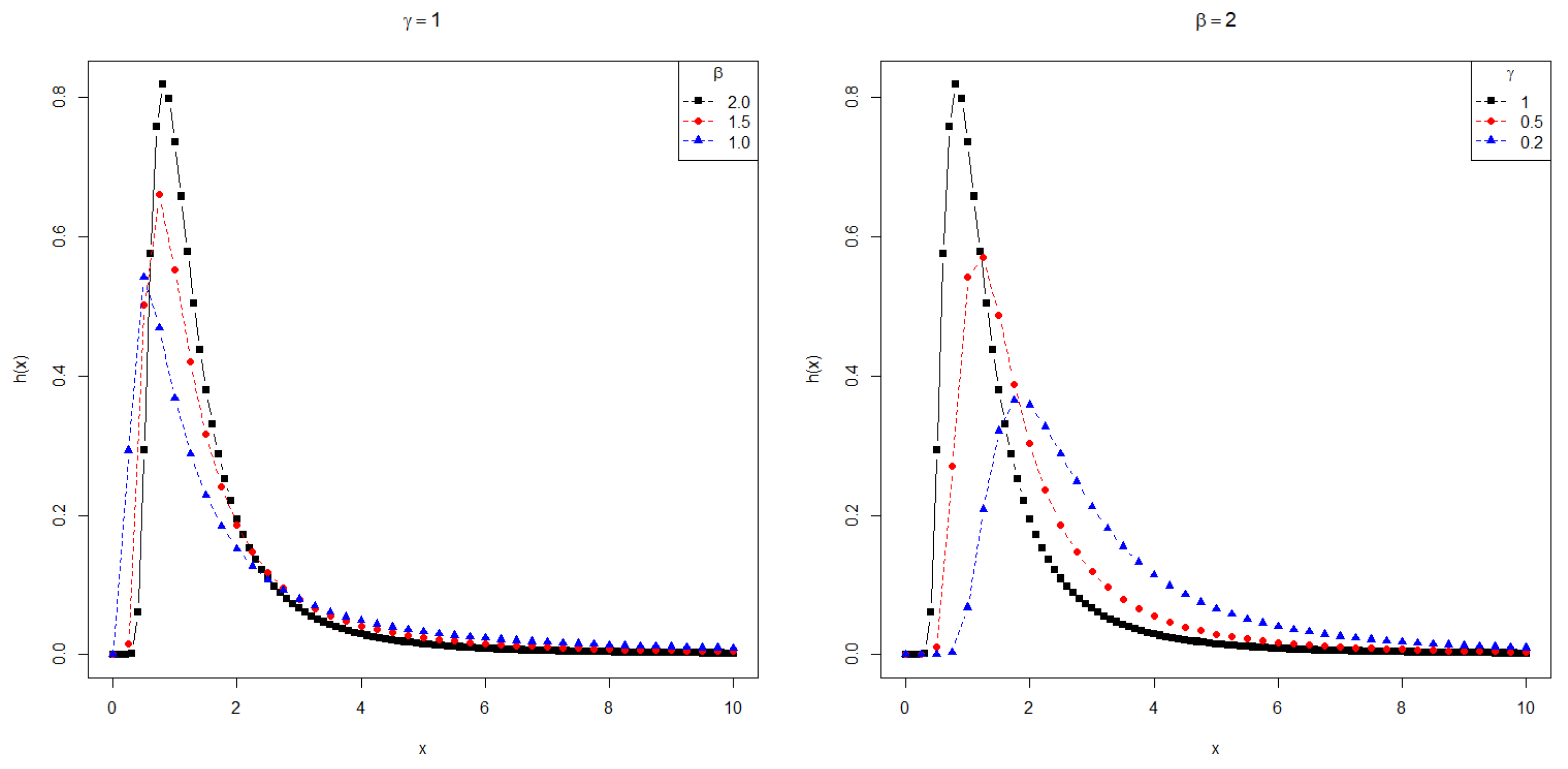
In Section 5, we apply the PDFs , and to the modeling of data with positive support. Furthermore, the supports of and depend on the parameters. Thus, the maximum likelihood estimation is not as straightforward as in the usual cases. Figure 1, Figure 2 and Figure 3 show the behavior of these densities for some choices of parameters, revealing the asymmetry and heavy tails of the PDFs.
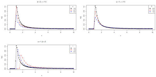
Figure 1.
Plots for the PDF .
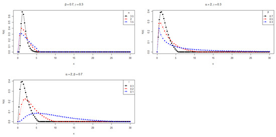
Figure 2.
Plots for the PDF .
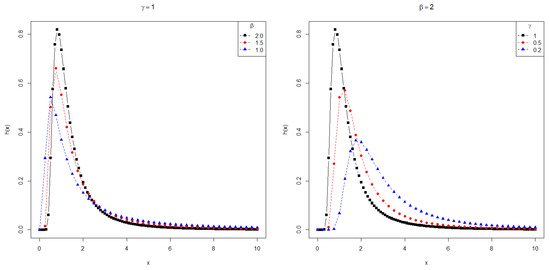
Figure 3.
Plots for the PDF .
3. Reliability for Three-Parameter -Max Stable Laws
In this section, the reliability of two independent three-parameter p-max stable random variables is derived in terms of the -function. In addition, with suitable parameter restrictions, the -function and a simpler form in terms of standard functions are obtained. Firstly, we consider the case of two independents .
Theorem 1.
Let Y and X be independent random variables, respectively, with CDF and , , and . Then,
provided that . In particular, if , then
When , R can be written explicitly as
Proof.
Secondly, we consider the case of two independents .
Theorem 2.
Let Y and X be independent random variables, respectively, with CDF and , , and . Then,
provided that . In particular, if , then
When , R can be written explicitly as
Proof.
Thirdly, we consider the case of two independents . The proofs of Theorems 3 and 4 are similar to those of Theorems 1 and 2, respectively. The details are omitted.
Theorem 3.
Let Y and X be independent random variables, respectively, with CDF and , , . Then,
provided that . In particular, if , then
When , R can be written explicitly as
Now, we consider the case of two independents .
Theorem 4.
Let Y and X be independent random variables, respectively, with CDF and , , and . Then,
provided that . In particular, if , then
When , R can be written explicitly as
Lastly, we consider the cases of two independents .
Theorem 5.
Let Y and X be independent random variables, respectively, with CDF , , and . Then,
- (a)
- for ,In particular, if , we have
- (b)
- for ,In particular, if , we have
Proof.
By combining all the Theorems from 1 to 4, it is possible to state the following Corollary:
Corollary 1.
Let Y and X be independent random variables, respectively, with CDF and , , , and . Then,
provided that . In particular, if , then
When , can be written explicitly as
We finish this section by noting that Theorems 1–5 can be generalized to random samples of a given F distribution that is in the domain of attraction of one of the p-max stable laws (see [20] for a complete characterization of the domains of attraction of the p-max stable laws). We describe below these generalizations.
4. Estimation
This section deals with parameter estimation for the p-max stable laws via a random optimization method and bootstrap confidence intervals.
Several authors (e.g., [8,9,11]) have estimated R by maximum likelihood. However, they relied on strong parameter restrictions to obtain an explicit form for R. Thus, the estimation of the parameters must be done jointly in the two samples. In our case, such restrictions were not necessary since we worked with expressions of R in terms of functions and , releasing any requirements about similar parameters between different samples.
To the best of our knowledge, there are few studies concerning parameter estimation, although the literature suggests several theoretical studies of p-max stable distributions (e.g., [21]). Here, we present a different approach for parameter estimation for the p-max stable laws.
We initially consider the PDF . For the other p-max stable laws, similar expressions are obtained using the PDFs presented in Section 2.2. Take as a sample of n observations. The likelihood function for the PDF is given by the following:
Note that if and only if for all . Then, we are not able to obtain the MLE explicitly, so an additional condition is required in the likelihood maximization process.
Remark 1.
The MLE of R is obtained using the invariance property of MLE. This is due to the Theorems 1–5 that describe R in terms of the function (which is an integral, hence a continuous and measurable function).
4.1. A Random Optimization Method for Approximating the MLE
Now, we describe the optimization methodology to be implemented for parameter estimation. Let be a likelihood function for which the maximum is assumed to be finite.
Algorithm 1 can find the point of maximum for which . Particularly, unlike conventional algorithms, random points in space are generated according to a generic distribution G (not necessarily uniform) on the parameter space . This allows us to introduce weights in some regions of the parameter space, as a kind of prior information.
Algorithm 1.
Let be independent and identically distributed random vectors with common distribution G on . Let be defined by
Step 1. and.
Step . Having defined , let be defined as
It was proved by [22] that for given and
that is, the -region of attraction of has been attained with probability , provided that the stop rule consists of terminating the algorithm for k such that
where m denotes the Lebesgue measure on . This means that with high probability, the algorithm reaches the desired maximum.
4.2. Bootstrap
The bootstrap method used in the next section to obtain bootstrap confidence intervals of R is described below.
Algorithm 2 describes the approach used in the next section to obtain bootstrap confidence intervals of R.
- Generate independent bootstrap samples and of sizes and , respectively.
- Compute the parameter estimation based on and .
- Obtain .
- Repeat steps times.
- The approximate confidence interval of R is given by , where and are the cumulative distribution function of .
Algorithm 2.
Let and be samples of sizes and , respectively, and a positive integer M.
- Step 1
- Generate independent bootstrap samples and .
- Step 2
- Compute the parameter estimation based on and .
- Step 3
- Obtain .
- Step 4
- Repeat steps to M times.
- Step 5
- The approximate confidence interval of R is given by , where and is the cumulative distribution function of .
5. Applications
In this section, we present Monte Carlo simulations as well as the modeling of two real situations involving football datasets and different-length carbon fibers. In order to enable readers to apply the methodology hereby proposed, the codes are available at a public repository [23] (link to be shared after acceptance).
5.1. Simulation Results
To illustrate the behavior of the random optimization method for approximating the MLE described in Algorithm 1 and to evaluate the performance of the estimate , we simulate random samples from CDFs , and (the other distributions could be used as well). The random samples are simulated using the generalized inverse of the CDFs applied to uniform random variables.
Values of , , and n are pre-specified, where n is the sample size and and are the parameters of the random optimization Algorithm 1.
Monte Carlo simulations were implemented in the language and environment for statistical computing R-4.4.0 [24], and each simulation outcome is based on samples of the parameter settings. In Table 1 and Table 2, we study the performance of the estimator when the PDF is . The PDFs and are treated in Table 3 and Table 4.

Table 1.
Mean, bias, and RMSE of for PDF (, , and ).
Table 2.
Mean, bias, and RMSE of for PDF (, , and ).
Table 3.
Mean, bias, and RMSE of for PDF (, , , and ).
Table 4.
Mean, bias, and RMSE of for PDF (, , , and ).
Remark 2.
(a) We start our study of simulations by PDF inspired by the applications presented in Section 5.2. As it will be seen, presented a good modeling performance in those cases.
(b) Recall that Algorithm 1 depends on parameters and on a distribution G on the parameter space Θ. To estimate , Θ must be a subspace of . We start by fixing the values , the search region for a fixed N value, and the uniform distribution on . Table 1 gives the results for different values of N. Changes in the constants and or on the upper bound of N could result in better or worse estimation. Table 2 shows results for and .
(c) If we want to search the entire parameter space, we should use another distribution with support on (e.g., gamma distribution).
For the simulation, we fix a search region of the parameter space , and for each line in the table
- 1000 random samples of and are simulated;
- for each simulation, the parameter is estimated, according to the likelihood function (34) and Algorithm 1;
- the mean of the 1000 corresponding (denote ) is obtained;
- the Bias and the Root Mean Squared Error (RMSE) are computed.
Table 1 shows that
- in general, the estimation of R had good results, indicated by the small value of the bias;
- the bias values were within the fixed range ;
- RMSE did not increase as we increased the search space .
Table 2 shows that by reducing the value of and while increasing n, we are able to reduce the RMSE values of Table 1, although we did not obtain significant reductions in the Bias values.
As in the case, for the PDFs and , the search space is . Thus, based on the results from Table 1 and Table 2 and on the computational difficulties with the increasing of N, we restrict our analysis for when the PDF is (for , which has only two parameters to be estimated, we keep ).
Table 3 and Table 4 present the mean, bias, and RMSE of for Monte Carlo simulations of X and Y from and , respectively, with , , and . For the simulations, we followed the same procedure used in the generation of Table 1.
Table 4 shows that the estimator has a better performance with a more precise estimation when the PDF is , also with less RMSEs. This was expected since there are only two parameters to be estimated from a random sample of X and two others from Y.
5.2. Real Dataset Applications
We now give two applications using real data analyzed earlier in the literature.
5.2.1. Medium Pass Completion Proportion
We use the data for the UEFA Champions League and 2022 FIFA World Cup datasets (Available at https://www.kaggle.com/ accessed on 13 February 2024) to illustrate the model developed in the preceding sections. We compare the medium pass completion proportion, that is, relative frequency of successful passes between 14 and 18 m - thus a number from 0 (none of the passes) to 1 (all the passes). These datasets were modeled before in [25]. For the convenience of the reader, datasets from UEFA (X) and FIFA (Y) are presented below:
and
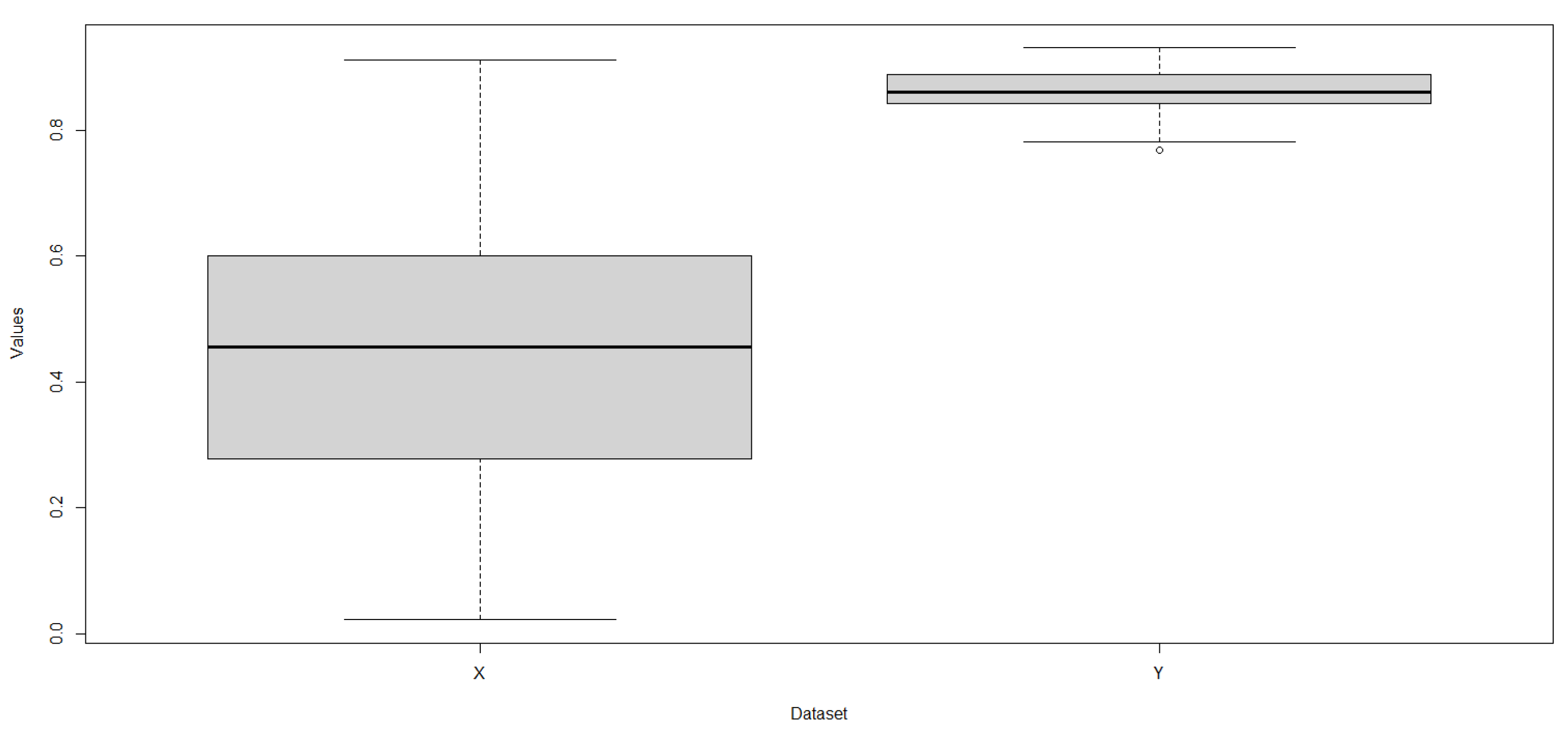
Descriptive statistics for X and Y are presented in Table 5. The boxplot shown in Figure 4 shows that X is more dispersed than Y and that Y values tend to be larger than X values (1st quartile of Y is greater than 3rd quartile of Y). Computing the value of the statistic R is important to probabilistically measure such a difference observed in the datasets.
Table 5.
Descriptive statistics for X and Y.
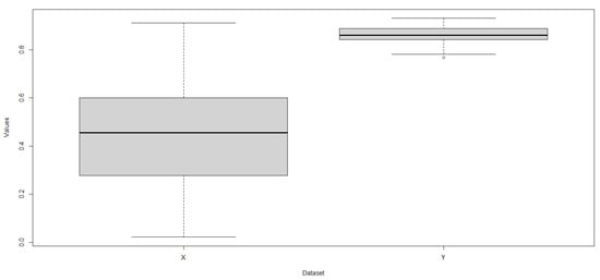
Figure 4.
Boxplots of X (left) and Y (right).
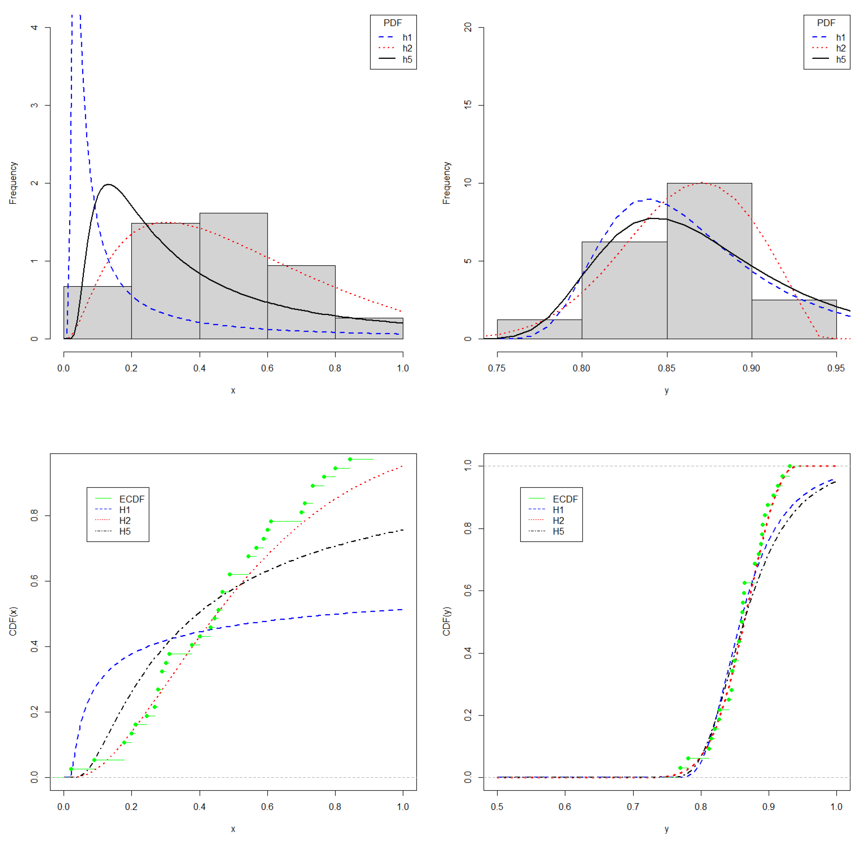
As the datasets have positive support, the PDF candidates to model such datasets are , , and . After estimating the parameters for the three distributions, the information criteria AIC, BIC, and EDC were applied, justifying the choice of PDF (see Table 6). This choice was also supported by the Kolmogorov–Smirnov test, whose p-values were and , for X and Y, respectively, indicating that we could not reject the null hypothesis that the CDF is . Figure 5 shows the fit of distributions to datasets.
Table 6.
Estimated parameters and information criteria for model selection.
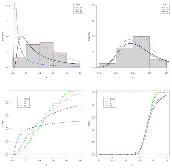
Figure 5.
Plots for X (left) and Y (right). On (top), histogram and fitted PDF; on (bottom), empirical CDF and fitted CDF.
Using Theorem 2, we obtain and the Bootstrap confident interval is . That indicates a high probability that the proportion of successful passes between 14 and 18 m in UEFA matches was lower than in FIFA.
5.2.2. Carbon Fibers
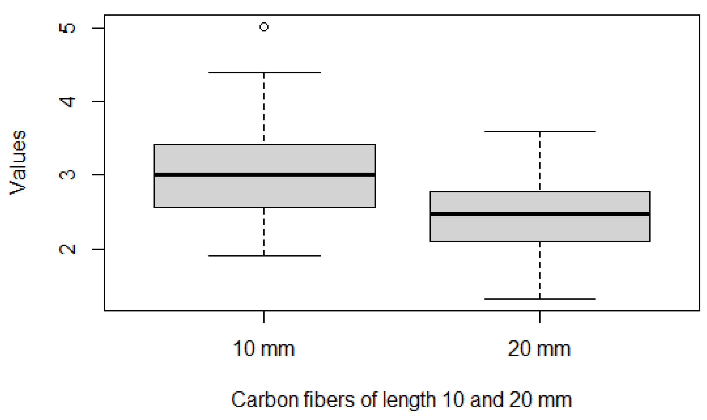
We now present an application of stress–strength probability calculation in the modeling and comparison of carbon fibers of length 20 mm (X) and 10 mm (Y). X and Y represent the strength data measured in GPa (Gigapascal) for single carbon fibers tested under tension and are also presented below in addition to being frequently used in the literature (e.g., [26]).
Table 7 and Figure 6 show that the descriptive profile of X and Y in which it is possible to observe that Y (carbon fibers of length 10 mm) tends to have greater values than X (carbon fibers of length 20 mm). This indicates that we expect a probability greater than .
Table 7.
Descriptive statistics for X and Y.
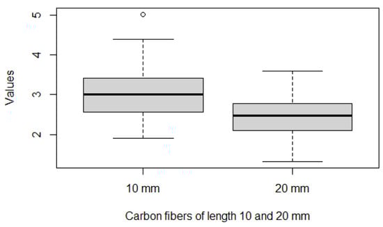
Figure 6.
Boxplots of X (left) and Y (right).
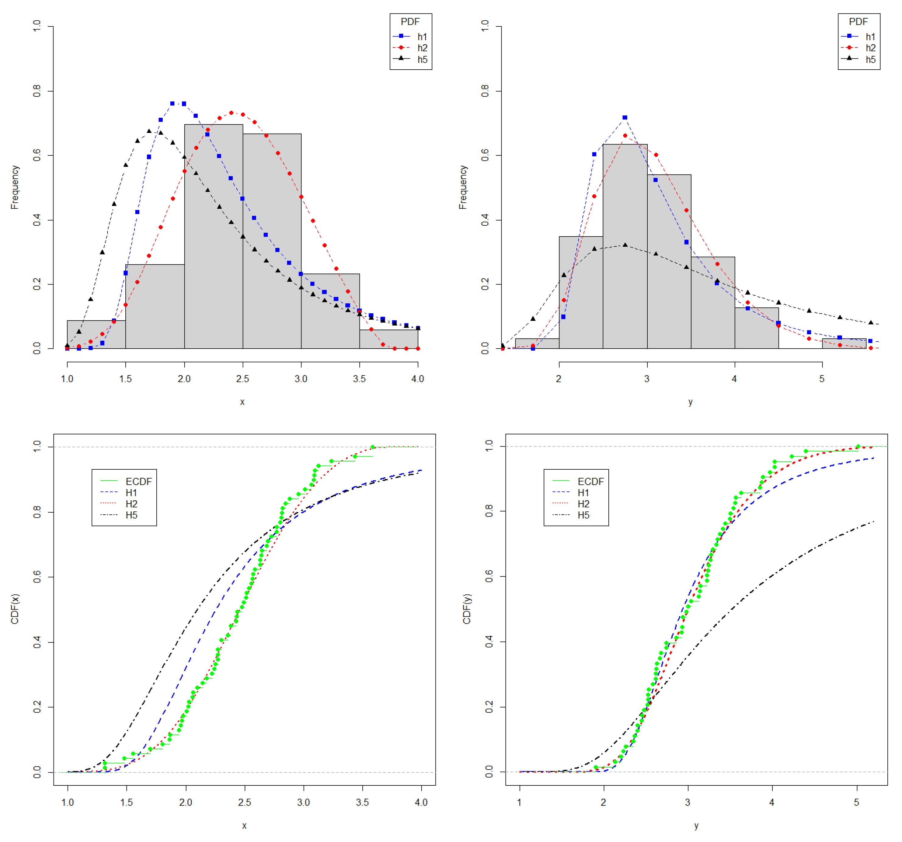
Considering that both X and Y are positive datasets, for the estimation of R, we must choose a p-max stable distribution with positive support. In this case, the candidates are , and , whose estimated parameters are shown in Table 8. In this same table, we also compared the fitted p-max distributions to the fittings obtained for the Weibull (WB) and the Exponentiated Weibull (EWB) distributions, with the latter being introduced in [27]. As a selection criterion for the best distribution, the AIC, BIC, and EDC criteria are evaluated, and we choose PDF . For the Y random variable, is found to be the best distribution according to all the metrics used. On the other hand, for the X random variable, by a small margin, the Weibull distribution is the best according to AIC e BIC; on the other hand, shows up as the best model according to EDC. Considering that EDC is a generalization of both AIC and BIC and that it encompasses an optimal penalization term, was chosen as the best model for the X random variable as well. The fit of the p-max distributions considered, in particular , to the data can be seen in Figure 7.
Table 8.
Estimated parameters and information criteria for model selection.
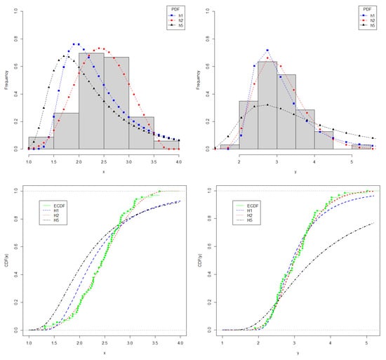
Figure 7.
Plots for X (left) and Y (right). On top, histogram and fitted PDF; on bottom, empirical CDF and fitted CDF.
We present the following conclusions:
- According to the AIC, BIC, and EDC criteria, PDF is the one that best fits data X and Y. This was expected since the same data were already modeled via Weibull distribution (see [11,28]) and having positive right endpoint, Theorem 3.1 in [20] establishes that would be the corresponding p-max stable distribution;
- The p-values of the Kolmogorov–Smirnov test are 0.9404 and 0.8390, respectively, which indicate that we cannot reject the null hypotheses that the X and Y CDFs are .
6. Conclusions
Our study aimed to investigate the estimation of the for independent marginals X and Y following p-max stable distributions. In order to do so, we obtained exact expressions for R. By using the new formulas proposed, direct and exact reliability applications are made possible for an important class of asymmetric distributions.
We discuss the application of a novel class of special functions, the so-called extreme value -function, which allows us to write the expressions of R explicitly and with minimal restrictions. In particular, by imposing additional parameter restrictions, R can be calculated in terms of -functions as well as even more compact expressions.
To the best of our knowledge, there are no previous works in the literature aiming to provide expressions and frameworks to perform reliability statistical inference for p-max stable distributions, and this work stands as a contribution by providing estimation methods based on stochastic optimization.
A restraint of our estimation method is the fact that it relies on compact search spaces for fixed N. However, we tested the performance of the proposed estimator by a Monte Carlo simulation study. Even though the search range N exponentially governs the computational effort required, the reported results reveal the correctness of the methodological approach hereby proposed.
Two applications to real datasets were carried out to show the performance of the p-max stable laws in reliability scenarios. Future work may explore other extreme value distributions and their reliability calculations, such as bimodal Weibull, bimodal Gumbel, bimodal GEV, and the extreme-value Birnbaum-Saunders distribution.
Overall, it is possible to summarize the strengths of the present paper as follows:
- General expressions were analytically derived for when X and Y follow three-parameter p-max stable laws with fewer parameter restrictions compared to previous results in the literature;
- A stochastic optimization procedure was proposed to build an estimator for R based on the novel expressions derived;
- The validity of the expressions and of the general methodological framework developed were demonstrated by Monte Carlo simulations;
- The suitability of the p-max distributions to model real datasets was attested by study cases.
On the other hand, the main weaknesses of the present paper are as follows:
- The stochastic optimization procedure relies on compact search spaces for fixed N, whose impact is exponential on the computational effort required;
- The amount of data used to illustrate the methodology and equations developed in the paper is limited; thus, the superiority of the p-max distributions over other possible models needs to be assessed in a case-by-case fashion.
Author Contributions
Conceptualization, F.S.Q.; methodology, F.S.Q., T.A.d.F., L.C.d.S.M.O. and P.N.R.; software, F.S.Q. and T.A.d.F.; validation, F.S.Q., T.A.d.F., L.C.d.S.M.O. and P.N.R.; formal analysis, F.S.Q., T.A.d.F., L.C.d.S.M.O. and P.N.R.; investigation, F.S.Q.; writing—original draft preparation, F.S.Q. and T.A.d.F.; writing—review and editing, L.C.d.S.M.O. and P.N.R.; supervision, P.N.R. All authors have read and agreed to the published version of the manuscript.
Funding
The APC was funded by University of Brasilia (Edital DPI/DPG/BCE Nº 01/2024).
Data Availability Statement
The data presented in the study are contained with the article and openly available in Zenodo at https://zenodo.org/doi/10.5281/zenodo.11416971.
Acknowledgments
The authors acknowledge the support provided by the University of Brasilia (UnB).
Conflicts of Interest
The authors declare no conflicts of interest.
References
- Kotz, S.; Lumelskii, Y.; Pensky, M. The Stress-Strength Model and Its Generalizations: Theory and Applications; World Scientific: Singapore, 2003. [Google Scholar]
- Rathie, P.; Freitas, S.; Nojosa, R.; Mendes, A.; Silva, T. Stress-Strength Reliability Models Involving H-Function Distributions. J. Ramanujan Soc. Math. Math. Sci. 2022, 9, 217–234. [Google Scholar]
- Rathie, P.N.; Ozelim, L.C.S.M. Exact and approximate expressions for the reliability of stable Lévy random variables with applications to stock market modelling. J. Comput. Appl. Math. 2017, 321, 314–322. [Google Scholar] [CrossRef]
- Quintino, F.S.; Oliveira, M.; Rathie, P.N.; Ozelim, L.C.S.M.; da Fonseca, T.A. Asset selection based on estimating stress-strength probabilities: The case of returns following three-parameter generalized extreme value distributions. AIMS Math. 2023, 9, 2345–2368. [Google Scholar] [CrossRef]
- Domma, F.; Giordano, S. A copula-based approach to account for dependence in stress-strength models. Stat. Pap. 2012, 54, 807–826. [Google Scholar] [CrossRef]
- Huang, C.Y.; Chin, W.C.B.; Wen, T.H.; Fu, Y.H.; Tsai, Y.S. EpiRank: Modeling Bidirectional Disease Spread in Asymmetric Commuting Networks. Sci. Rep. 2019, 9, 5415. [Google Scholar] [CrossRef]
- Nadarajah, S. Reliability for extreme value distributions. Math. Comput. Model. 2003, 37, 915–922. [Google Scholar] [CrossRef]
- Abbas, K.; Tang, Y. Objective Bayesian analysis of the Frechet stress–strength model. Stat. Probab. Lett. 2014, 84, 169–175. [Google Scholar] [CrossRef]
- Jia, X.; Nadarajah, S.; Guo, B. Bayes estimation of P(Y < X) for the Weibull distribution with arbitrary parameters. Appl. Math. Model. 2017, 47, 249–259. [Google Scholar]
- Krishnamoorthy, K.; Lin, Y. Confidence limits for stress–strength reliability involving Weibull models. J. Stat. Plan. Inference 2010, 140, 1754–1764. [Google Scholar] [CrossRef]
- Kundu, D.; Raqab, M. Estimation of R = P(Y < X) for three-parameter Weibull distribution. Stat. Probab. Lett. 2009, 79, 1839–1846. [Google Scholar]
- Aryal, G.R.; Tsokos, C.P. On the transmuted extreme value distribution with application. Nonlinear Anal. Theory Methods Appl. 2009, 71, e1401–e1407. [Google Scholar] [CrossRef]
- Vila, R.; Niyazi Çankaya, M. A bimodal Weibull distribution: Properties and inference. J. Appl. Stat. 2022, 49, 3044–3062. [Google Scholar] [CrossRef]
- Otiniano, C.; Vila, R.; Brom, P.; Bourguignon, M. On the Bimodal Gumbel Model with Application to Environmental Data. Austrian J. Stat. 2023, 52, 45–65. [Google Scholar] [CrossRef]
- Otiniano, C.E.; Paiva, B.S.; Vila, R.; Bourguignon, M. A bimodal model for extremes data. Environ. Ecol. Stat. 2023, 30, 261–288. [Google Scholar] [CrossRef]
- Pantcheva, E. Limit theorems for extreme order statistics under nonlinear normalization. In Stability Problems for Stochastic Models; Springer: Berlin/Heidelberg, Germany, 1985; pp. 284–309. [Google Scholar]
- Feng, B.; Chen, S. On large deviations of extremes under power normalization. Stat. Probab. Lett. 2015, 99, 27–35. [Google Scholar] [CrossRef]
- Mathai, A.; Saxena, R.; Haubold, H. The H-Function: Theory and Applications; Springer Science & Business Media: Berlin/Heidelberg, Germany, 2009. [Google Scholar]
- Rathie, P.N.; Ozelim, L.C.d.S.M.; Quintino, F.; Fonseca, T.A.d. On the Extreme Value H-Function. Stats 2023, 6, 802–811. [Google Scholar] [CrossRef]
- Mohan, N.; Ravi, S. Max domains of attraction of univariate and multivariate p-max stable laws. Theory Probab. Its Appl. 1993, 37, 632–643. [Google Scholar] [CrossRef]
- Barakat, H.; Nigm, E.; Khaled, O. Extreme value modeling under power normalization. Appl. Math. Model. 2013, 37, 10162–10169. [Google Scholar] [CrossRef]
- Dorea, C.C. Stopping Rules for a Random Optimization. SIAM J. Control Optim. 1990, 28, 841–850. [Google Scholar] [CrossRef]
- Quintino, F.; Rathie, P.; Ozelim, L.; Fonseca, T. Codes for Estimation of P(X < Y) stress–strength reliability measures for a class of asymmetric distributions: The case of three-parameter p-max stable laws. Zenodo 2024. Available online: https://zenodo.org/records/11416972 (accessed on 13 February 2024).
- R Core Team. R: A Language and Environment for Statistical Computing; R Foundation for Statistical Computing: Vienna, Austria, 2022. [Google Scholar]
- Vila, R.; Balakrishnan, N.; Saulo, H.; Zörnig, P. Family of bivariate distributions on the unit square: Theoretical properties and applications. J. Appl. Stat. 2023, 51, 1729–1755. [Google Scholar] [CrossRef]
- Valiollahi, R.; Asgharzadeh, A.; Raqab, M.Z. Estimation of P (Y < X) for Weibull distribution under progressive Type-II censoring. Commun. Stat.-Theory Methods 2013, 42, 4476–4498. [Google Scholar]
- Mudholkar, G.; Srivastava, D. Exponentiated Weibull family for analyzing bathtub failure-rate data. IEEE Trans. Reliab. 1993, 42, 299–302. [Google Scholar] [CrossRef]
- Kundu, D.; Gupta, R. Estimation of P[Y < X] for Weibull distributions. IEEE Trans. Reliab. 2006, 55, 270–280. [Google Scholar] [CrossRef]
Disclaimer/Publisher’s Note: The statements, opinions and data contained in all publications are solely those of the individual author(s) and contributor(s) and not of MDPI and/or the editor(s). MDPI and/or the editor(s) disclaim responsibility for any injury to people or property resulting from any ideas, methods, instructions or products referred to in the content. |
© 2024 by the authors. Licensee MDPI, Basel, Switzerland. This article is an open access article distributed under the terms and conditions of the Creative Commons Attribution (CC BY) license (https://creativecommons.org/licenses/by/4.0/).